the Creative Commons Attribution 4.0 License.
the Creative Commons Attribution 4.0 License.
 | 02 Aug 2019
Seasonal and regional variations of sinking in the subpolar North Atlantic from a high-resolution ocean model
Juan-Manuel Sayol
Henk Dijkstra
Caroline Katsman
Previous studies have indicated that most of the net sinking associated with the downward branch of the Atlantic Meridional Overturning Circulation (AMOC) must occur near the subpolar North Atlantic boundaries. In this work we have used monthly mean fields of a high-resolution ocean model (0.1∘ at the Equator) to quantify this sinking. To this end we have calculated the Eulerian net vertical transport (W∑) from the modeled vertical velocities, its seasonal variability, and its spatial distribution under repeated climatological atmospheric forcing conditions. Based on this simulation, we find that for the whole subpolar North Atlantic W∑ peaks at about −14 Sv at a depth of 1139 m, matching both the mean depth and the magnitude of the meridional transport of the AMOC at 45∘ N. It displays a seasonal variability of around 10 Sv. Three sinking regimes are identified according to the characteristics of the accumulated W∑ with respect to the distance to the shelf: one within the first 90 km and onto the bathymetric slope at around the peak of the boundary current speed (regime I), the second between 90 and 250 km covering the remainder of the shelf where mesoscale eddies exchange properties (momentum, heat, mass) between the interior and the boundary (regime II), and the third at larger distances from the shelf where W∑ is mostly driven by the ocean's interior eddies (regime III). Regimes I and II accumulate ∼90 % of the total sinking and display smaller seasonal changes and spatial variability than regime III. We find that such a distinction in regimes is also useful to describe the characteristics of W∑ in marginal seas located far from the overflow areas, although the regime boundaries can shift a few tens of kilometers inshore or offshore depending on the bathymetric slope and shelf width of each marginal sea. The largest contributions to the sinking come from the Labrador Sea, the Newfoundland region, and the overflow regions. The magnitude, seasonal variability, and depth at which W∑ peaks vary for each region, thus revealing a complex picture of sinking in the subpolar North Atlantic.
- Article
(11423 KB) -
Supplement
(13875 KB) - BibTeX
- EndNote


The Atlantic Meridional Overturning Circulation (AMOC) is a fundamental component of the Earth's climate system (Lozier, 2012; Buckley and Marshall, 2016). Over the last few decades the traditional view of an ocean conveyor with an upper poleward current transporting warm waters to higher latitudes, and a downward branch with intermediate and deeper denser waters that originate in the regions of deep convection and move toward the Equator (Broecker, 1987, 1991), has been revised.
First, it became apparent that eddies actively mediate between the upper and lower limbs of the AMOC (Lozier, 2010). As a consequence, the Deep Western Boundary Current (DWBC) presents large spatiotemporal variability, as the flow splits in the North Atlantic (near 50∘ N) in the well-known western current aligned with the boundary (Stommel and Arons, 1959) and other more elusive interior paths (Bower and Hunt, 2000; Bower et al., 2009). Similarly, at the surface, the pathways of the North Atlantic Current that connect the subtropical gyre with the subpolar gyre are still not well established, as evidenced by the trajectories of surface drifters (Brambilla and Talley, 2006) and by estimates of the inter-gyre exchange (Rypina et al., 2011).
Second, the earlier idea that strong open-ocean convection – e.g., in the interior of the Labrador, Irminger, and Greenland seas – is accompanied by large-scale sinking of waters, and that this downwelling represents the largest part of the sinking related to the AMOC, has been abandoned. The explanation for this is that once the winter cooling has preconditioned the convection site through a prolonged buoyancy loss, the vertical transport associated with small-scale (∼1 km) deep convective plumes is mostly compensated for by a nearby rise of waters so that little vertical mass transport is expected (Marshall and Schott, 1999; Send and Marshall, 1995). Moreover, these regions of deep convection are highly localized, with length scales of 500 km or less. This implies that the horizontal gradient in planetary vorticity across the convection region is small. In order to balance the vorticity changes associated with substantial sinking in the geostrophic ocean interior, an unrealistically strong northward current would be required (Spall and Pickart, 2001). Instead, previous studies have shown that the Eulerian net sinking (in depth space) associated with the lower branch of the AMOC must occur near the boundaries, where the flow is subject to non-geostrophic dynamics. Thus, at the topographic slopes a richer vorticity balance arises with a dissipation term that compensates for the vertical stretching of planetary vorticity induced by the sinking (Spall and Pickart, 2001; Spall, 2004, 2008; Brüggemann et al., 2017). As a result, higher rates of sinking are attainable near the boundaries of marginal seas.
Spall and Pickart (2001) and Pedlosky and Spall (2005) analyzed the sinking along a straight boundary current subject to buoyancy loss. They found that a flow in thermal-wind balance develops, with a density gradient that spirals with depth. Such a spiraling structure induces strong vertical movements, which they found to be proportional to the alongshore density gradient and the mixed layer depth. With a two-layer approach, Straneo (2006) studied a boundary current surrounding denser interior waters as a representation of the Irminger Current waters flowing around the perimeter of the Labrador Sea. In her model net sinking appears in the boundary layer as the boundary current loses buoyancy along the perimeter. She also found that larger alongshore density gradients give rise to more sinking. Consistently Cenedese (2012) came to a similar conclusion from laboratory experiments in a tank. However, the North Atlantic is not the only place where sinking predominantly takes place near the boundaries. As pointed out by the recent work of Waldman et al. (2018), significant sinking occurs in the first 50 km off the coast in the Mediterranean Sea, though it is much smaller than in the North Atlantic ( Sv, where ). At this location, sinking is catalyzed by the existence of a western boundary current that densifies along its way around the basin, a strong winter cooling in the interior due to northerly winds, and an active near-shelf eddy field.
More recently, Katsman et al. (2018) estimated the net sinking in the North Atlantic from model simulations at a depth chosen to match the maximum of the overturning streamfunction (at 1060 m), well below the mixed layer depth. They computed the net sinking over the time-averaged fields of two hindcasts based on the same ocean model (ORCA) and atmospheric forcing. The two simulations covered the period 1958–2001 and had a different horizontal resolution (0.25 and 1∘ for ORCA025 and ORCA1, respectively). Their results showed a significant net sinking along the boundaries, much higher than in the interior. Notably, the finer-resolution model displayed 8 Sv more net sinking along the perimeter than the lower-resolution version (−20 and −12 Sv, respectively). However, the contribution of overflow waters to the total budget of net sinking along the selected perimeter was nearly the same in absolute terms, with average amounts of −7.6 and −7.4 Sv for the coarser- and the finer-resolution simulation, respectively. Hence, the large differences in sinking between the two simulations are mostly attributed to the boundary region. According to the authors, this difference may be due to the fact that the finer-resolution model is eddy permitting. Thus, ageostrophic eddy-driven processes may also play an important role in boundary sinking. For instance, eddy-induced heat fluxes significantly increase the lateral heat exchange between the cooler interior and the warmer boundary, cooling the boundary current on its way and then enhancing the alongshore density gradient (Spall, 2011). Also, as pointed out by Spall (2010), eddy vorticity fluxes and dissipation play an important role in balancing the vertical stretching of planetary vorticity induced by sinking in a convective basin.
In order to better understand the contribution of geostrophic and ageostrophic processes to sinking, Brüggemann and Katsman (2019) used an idealized model with fine resolution (3 km in the horizontal), which is able to mimic the basic features of the Labrador Sea: a cyclonic boundary current circulating along a semicircular basin, with a small part dominated by a steeper topographic slope (change in depth of 3000 m in a few tens of kilometers), resulting in the generation of a vigorous eddy field. Stronger sinking was found onto and near the sharp topographic feature than in any other place in the domain. Likewise, the recent work of Georgiou et al. (2019) highlights the importance of eddy-driven transport using an idealized eddy-resolving model of the Labrador basin. Among other aspects, this study demonstrates that the total amount of sinking is sensitive to changes in the eddy pathways. It must be stressed here that the above idealized studies assumed closed basins, while in reality open boundaries exist and exchanges between the North Atlantic and Arctic occur. Overflows also contribute significantly to the net sinking, as shown in Katsman et al. (2018). However, they are governed by different dynamics (e.g., Shapiro and Hill, 1997; Yankovsky and Legg, 2019).
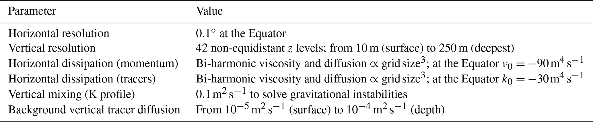
Table 1Summary of POP model key parameters used in the simulation (see Maltrud et al., 2010; Weijer et al., 2012; Brunnabend and Dijkstra, 2017, for details).
This work adds a new dimension of complexity to existing studies by investigating how the net sinking in the North Atlantic changes seasonally and regionally. Despite the promising first results of the Overturning in the Subpolar North Atlantic Program – OSNAP (Lozier et al., 2017, 2019; Kornei, 2018; Holliday et al., 2018), the scarcity of measurements below the surface still necessitates the use of numerical models to provide more insight into the spatiotemporal variability of sinking and to grasp the physical processes behind its dynamics. To this end, we use an ocean-only eddy-resolving numerical simulation with a nominal resolution of 0.1∘ under a repeated climatological annual atmospheric forcing, not adding the additional complexity of historical variations (e.g., variations at interannual or inter-decadal scales) in surface forcing. Since the degree of buoyancy loss, the topographic configuration, and the oceanic circulation differ among the North Atlantic sub-basins, a complex repartitioning of sinking is anticipated. Therefore, we separately evaluate the seasonality and the distribution of sinking at different spatial scales including the marginal seas and overflow areas in the basin. In addition, the connection between sinking and the AMOC is addressed throughout the paper.
The remainder of this paper is structured as follows: in Sect. 2 we introduce the numerical simulation and assess the ability of the model to reproduce a realistic AMOC; in Sect. 3 we consider the main characteristics and the seasonal variability of sinking in the entire subpolar North Atlantic; in Sect. 4 we evaluate similarities and differences between sinking in the marginal seas, overflow regions, and midlatitude seas of the subpolar North Atlantic based on their different bathymetric profiles and driving local dynamical processes; and in Sect. 5 we show that in our simulation the connection between sinking variations and AMOC change fades when the dominant seasonal signal is removed. To conclude, in Sect. 6 we summarize and discuss the most significant findings.
The model setup is based on a configuration of the Parallel Ocean Program (POP) model (Maltrud et al., 2008; Smith et al., 2010). This model solves the primitive equations on a tripolar curvilinear grid with a nominal horizontal resolution of 0.1∘ at the Equator and 42 z layers in the vertical down to a depth of 6000 m. The vertical resolution ranges from 10 m at the surface to 250 m for the deepest layers. The bottom topography is described by partial bottom cells (Adcroft et al., 1997). The atmospheric forcing fields (wind, heat fluxes, and precipitation) are applied by repeating a prescribed annual cycle from the Coordinated Ocean Reference Experiment (CORE) forcing dataset (Large and Yeager, 2004). Observed river runoff fields are also included. Table 1 shows the value of some key model parameters. The simulation analyzed here is a subset of a longer control run already employed by Brunnabend and Dijkstra (2017) – see the latter for more details on this simulation.
2.1 Model data and general performance
We use 15 years of three-dimensional monthly mean fields of velocity, potential density, temperature, and salinity for our analysis. Other two-dimensional variables such as bottom depth, the area and volume of grid cells and monthly mean fields of mixed layer depth are also utilized. Since this study focuses on the seasonal timescale and because the forcing is annually repeated, 15 years is sufficient to provide robust results. The period selected, corresponding to years 260–274 in the simulation time frame, is chosen well after the spin-up years. We note that interannual and larger timescales of variability are not included in our prescribed repeated annual forcing. This does not alter the validity of our analysis at seasonal scales since the annual cycle of winds and heat fluxes is dominant. Maps with mean ocean currents for the North Atlantic Ocean at depths of 5 and 1139 m (Fig. S1) show a realistic strength and location of the Gulf Stream and other subpolar boundary currents, taking into account the resolution of the model. Previous work using the same model in a similar setup found a well-represented distribution of currents, kinetic energy, and water-mass properties at basin scale (Maltrud et al., 2010; Weijer et al., 2012; Brunnabend and Dijkstra, 2017). Moreover, the modeled mixed layer depth qualitatively matches the spatial pattern derived from Argo floats (Våge et al., 2009; Holte et al., 2017), whereby the areas of deepest convection are found in the southwest Labrador Sea, in the Greenland Sea, and around the Iceland–Scotland Ridge. However, the modeled data show some delay in reaching the deepest mixed layer depth in the Labrador Sea (March against April) and tend to overestimate the observed mean values in some areas (compare Figs. S2 and S3). We partly attribute this to the use of repeated normal-year forcing conditions for wind and heat fluxes. We also note that the spatial coverage by Argo floats is still scarce and hence gridded fields are coarser than model data. In addition, both results are sensitive to the algorithm used to compute the mixed layer depth (de Boyer Montégut et al., 2004).
2.2 Overturning streamfunction
The overturning streamfunction (ψo) is a measure of the AMOC strength. With this metric northward and southward flows can be identified, and the depth at which the transport reaches its maximum. ψo is determined from the vertical integral of the zonally integrated meridional velocity at the southern boundary of our domain and the running meridional integral of the zonally integrated vertical velocity, i.e.,
where and are the meridional and vertical ocean velocity components, y0 is latitude of the southern boundary (selected at N), is the ocean bottom depth, and xw and xe are the western and eastern boundaries of the North Atlantic Ocean, respectively (Fig. 1a). The model simulation analyzed here yields a maximum time-averaged overturning streamfunction of 25.6 Sv near 35∘ N, whereas the modeled ψo at the RAPID array location (26∘ N) shows a maximum time-averaged transport of 22.3±1.9 Sv (Fig. 1b, blue line). This value is within the interval of uncertainty of the annual mean RAPID array observations prior to 2008, 18.8±4.3 Sv (Cunningham et al., 2007; Kanzow et al., 2010), and slightly larger than observations if we consider a longer RAPID period (April 2004–January 2017) with 17.0±1.9 Sv (the uncertainty is the standard deviation). Recent model-based results from Sinha et al. (2018) indicate that the RAPID array may be underestimating the transport by about 1.5 Sv due to structural errors in the array setup. Not surprisingly, our simulation is less successful in reproducing the range of variability of annual averages at the RAPID array (April 2004–January 2017), underestimating this variability by almost 5 Sv, with a range of 3.2 Sv against the measured 7.9 Sv (Smeed et al., 2014, 2018). This underestimation is likely due to the use of seasonal mean wind forcing conditions for which the atmospheric high-frequency variability has been partially filtered. Finally, the depth of the maximum time-averaged ψo is 1139 m (Fig. 1a), very close to the depth found at the RAPID array location at about 1100 m (Smeed et al., 2014, 2018). At 45∘ N (red line in Fig. 1b), the modeled AMOC is around 8 Sv weaker than at the RAPID array location but presents a more pronounced seasonal cycle (around 10 Sv), with the maximum in August and the minimum in February. Results from two dedicated campaigns in different years covering the OSNAP sections (∼50–60∘ N) provided a similar range of variability for ψo, ∼10–20 Sv (Holliday et al., 2018). The recent first assessment of the OSNAP observations by Lozier et al. (2019) yields a mean estimate of ψo that is smaller than our mean ψo at 45∘ N (around 6 Sv smaller) but that compares well with our mean modeled results at 55∘ N (8.0±0.7 Sv versus 8.1±2.4 Sv; not shown). The depths of maximum ψo are located at around 1000 m for the OSNAP observations and at around 1100 m for our simulation for both 45 and 55∘ N. Their results do not show a clear seasonal signal in the AMOC, while our simulation shows a marked seasonality in ψo for 45∘ N (∼10 Sv) and 55∘ N (∼8 Sv). We partly attribute this difference between the observations and our modeled results to the short OSNAP time series (only 21 months, from August 2014 to April 2016) and to the fact that we are using normal forcing conditions with a dominant seasonal signal without high-frequency wind variability. Nevertheless, a stronger transport in summer than in winter can be inferred from the OSNAP observations (Lozier et al., 2019), which is in agreement with our modeled results. Therefore, we conclude that our simulation displays an AMOC with reasonable mean transport and variability, as well as a well-located core in depth.
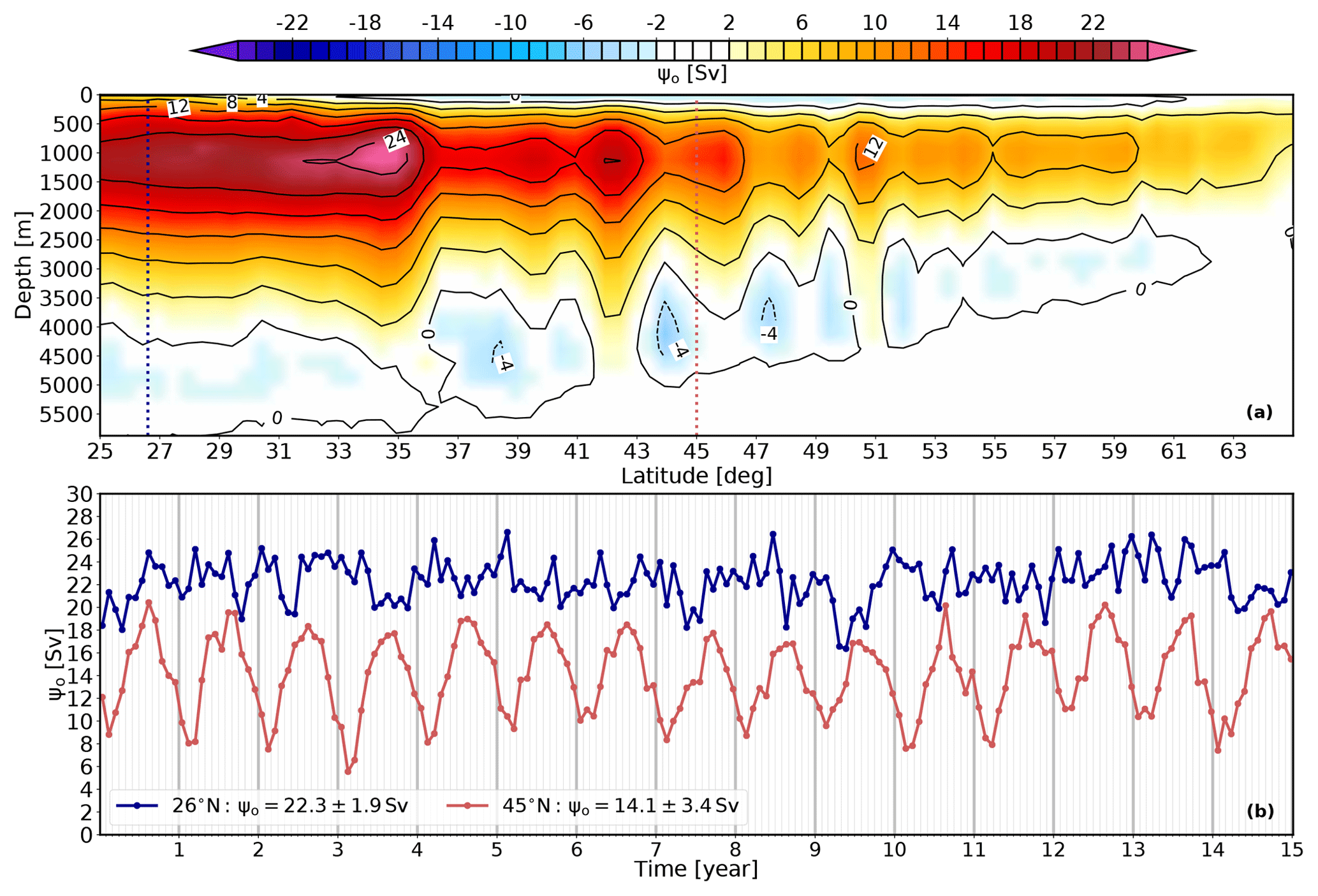
Figure 1(a) The 15-year average (years 260–274) overturning streamfunction, ψo(y, z), for the North Atlantic Ocean. (b) Time series of maximum overturning streamfunction at 26∘ N (blue) and 45∘ N (red); positions are also indicated by dashed lines in Fig. 1a. .
The structure of the AMOC streamfunction (Fig. 1a) indicates that there is a decrease in the amount of transport between the North Atlantic midlatitudes and the subpolar region that, by mass conservation, must be reflected in the magnitude of the vertical transport. However, such figures only provide a two-dimensional view of the overturning circulation in the subpolar North Atlantic. In this study we analyze the complex full structure of the circulation by characterizing spatial and seasonal variations in the sinking. In Sect. 3.1 we present the spatial distribution of modeled vertical velocities, which we use to compute the net vertical transport for the subpolar North Atlantic Ocean, its seasonal variability, and its vertical structure. In Sect. 3.2 a distinction in sinking regimes is proposed based on the differences in the net vertical transport between the near-shelf and the interior regions. To conclude this section, we discuss our results in light of earlier studies.
3.1 Vertical structure of sinking
A map of the mean distribution of the maximum vertical velocities (, the sign is conserved) obtained from the monthly mean fields in the North Atlantic (Fig. 2a) shows a spatial pattern characterized by strong velocities mostly confined to the boundaries. This is in line with results from idealized models (Spall and Pickart, 2001; Spall, 2004, 2010; Straneo, 2006; Georgiou et al., 2019; Brüggemann and Katsman, 2019) and global ocean models (Katsman et al., 2018). may reach values of over 150 m d−1, in good agreement with glider-based observations (Frajka-Williams et al., 2011). Figure 2b shows the depth at which the velocities are most intense; the black points mark where is larger than 80 m d−1. Most of the strong vertical velocities are found at a depth around 1000 m (black contour in Fig. 2a) close to the boundaries. These strong vertical velocities cannot be considered noise since they show a coherent spatial pattern along the bathymetric contours, and their standard deviation is several times smaller (square root of variance shown in Fig. 2c, about 30 m d−1) than their mean value. At some locations, alternating patterns of upward and downward motions are found (Fig. 2a, southeast of Greenland). As shown later, water is forced to move up and down there due to the dynamical restrictions imposed by the full vorticity balance on topographic slopes (see, e.g., Spall, 2010). The positive and negative alternations offshore of the Flemish Cap and in the interior of the Greenland and Norwegian seas must have a different cause. In the case of the Flemish Cap, they occur at the edges of eddies (Fig. S4), and the depth of largest sinking is below 2000 m (Fig. 2b, also in the interior of the Norwegian and Greenland seas), which indicates these eddies are deep and possibly have a strong barotropic component. Indeed, the high variance of vertical velocities in the surroundings of the Flemish Cap (σ2(w)) is a reflection of the existence of an active eddy field throughout the year (Fig. 2c). The subsurface EKE also shows this signal (Fig. S5).
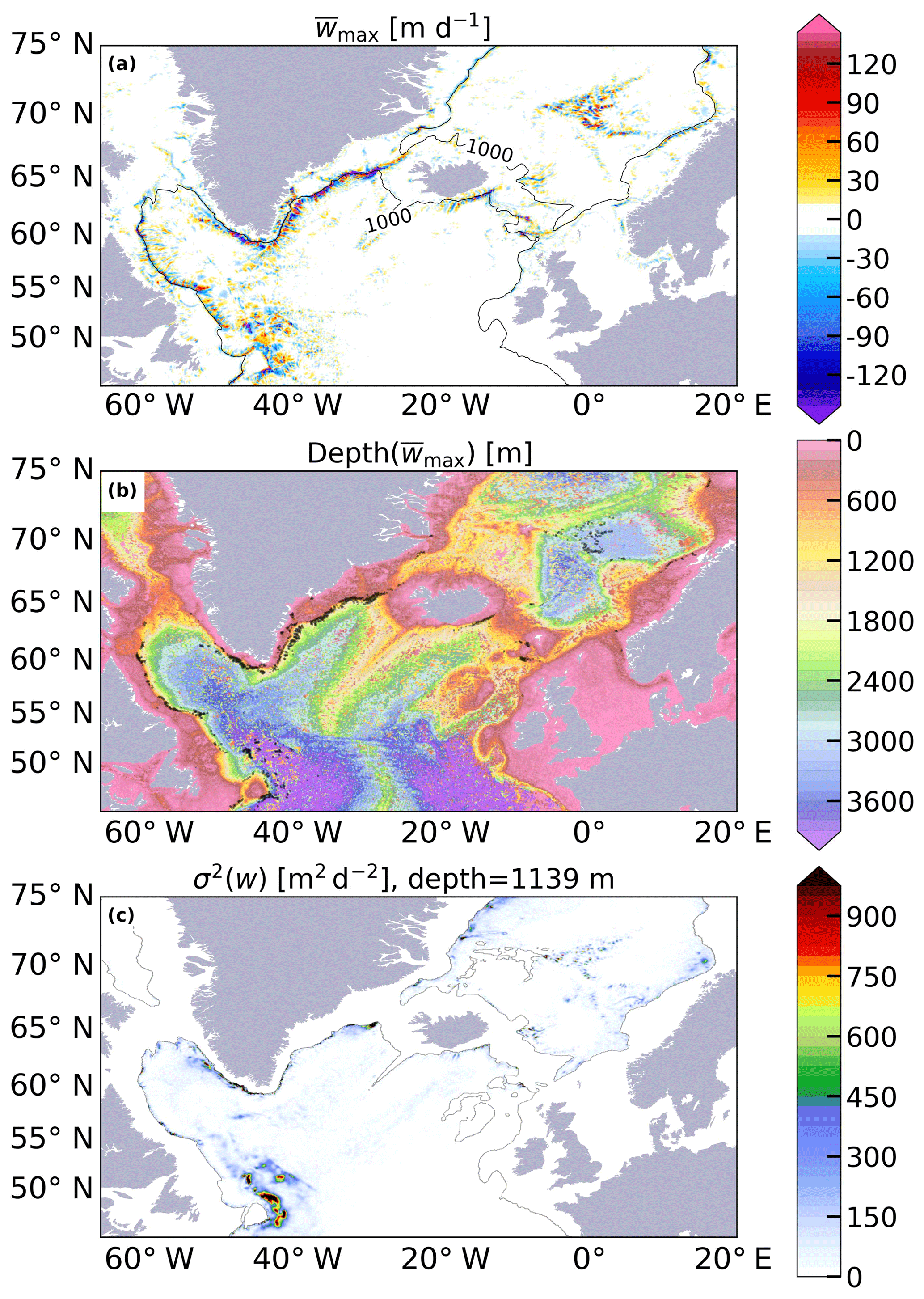
Figure 2(a) The 15-year maximum mean vertical velocity () for the North Atlantic Ocean. Contour lines denote the two longest 1000 m bathymetric features, which are separated by the Denmark Strait and the Iceland–Scotland Ridge. (b) Depth of plotted in (a). Black dots mark those grid cells in which is larger than 80 m d−1. (c) 15-year variance of vertical velocity (σ2(w)) at a depth of 1139 m. This depth corresponds to the depth at which the vertical transport associated with the AMOC peaks.
To assess the magnitude and the depth at which the near-boundary sinking occurs, we sum the local vertical transport for the entire subpolar North Atlantic. First, we calculate the vertical transport for all model grid points and for every depth as , where A(x, y) is the area of the grid cell, which depends on its location (x, y) in our curvilinear grid. Second, we sum W over the horizontal domain shown in Fig. 2. We will refer to this net vertical transport as W∑ for simplicity. The vertical profile of W∑ is shown in Fig. 3a. Large negative values of W∑ are found between 500 and 2700 m, with the strongest downward transport located at a depth of 1139 m. By mass conservation we expect that W∑ in our domain will be closely related to the transport at the southern boundary of the domain (45∘ N) since the North Atlantic Current is the dominant feature in the basin, although some mass contribution from the Arctic Ocean at 75∘ N and through the Davis Strait can be expected (Rudels et al., 2005; Azetsu-Scott et al., 2012). A comparison between time series of minimum W∑ and the maximum ψo (Fig. 1b) yields an excellent agreement in magnitude: 14.1±3.4 Sv against Sv (Figs. 1b and 3a). If we compare the reversed time series of ψo at 45∘ N (solid red line in Fig. 3b) with the time series of W∑ at the depth of minimum W∑ (solid purple line), it is clear that the seasonal signal also matches, with the minimum W∑ in summer (August) and the maximum in winter (February). The broadest range of variability (maximum minus minimum) is around 12 Sv in both time series at ∼1100 m of depth. If we repeat the comparison after removing the seasonal signal from both time series (dashed lines in Fig. 3b), the high correlation persists (>0.9) but with a reduced maximum range of variability of 5 Sv.
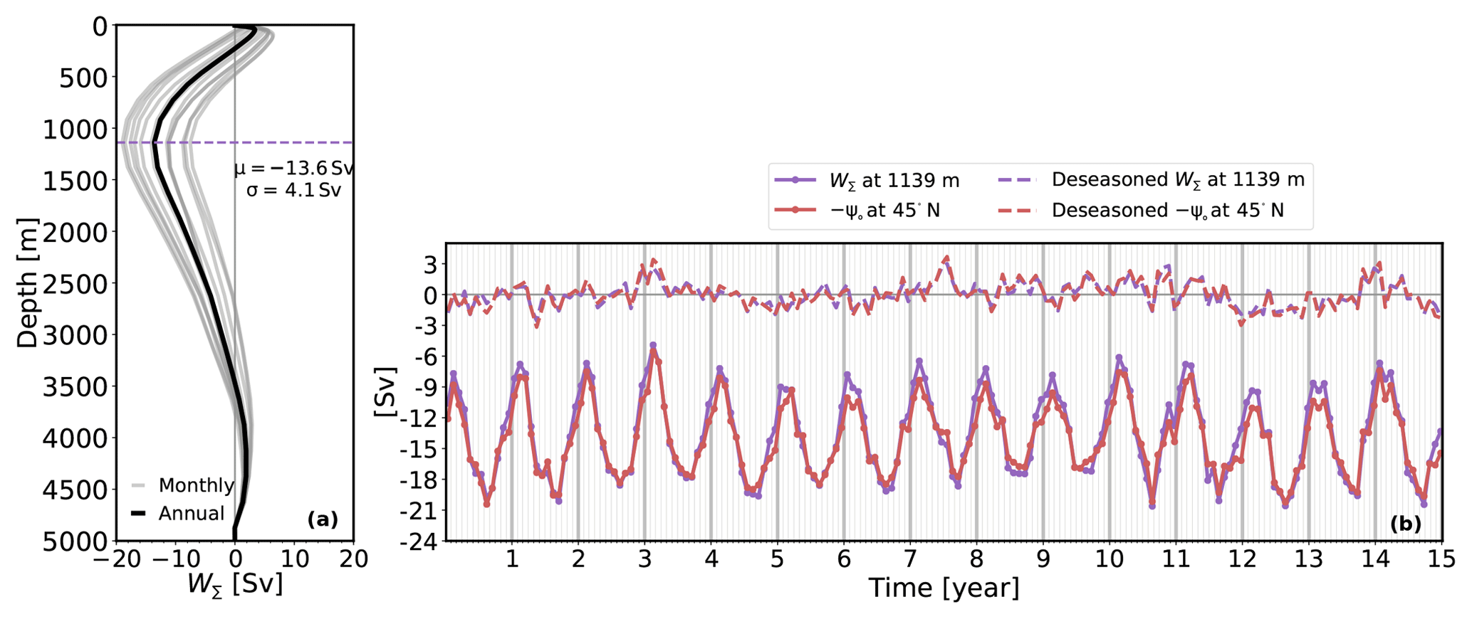
Figure 3(a) Mean profile of the net vertical transport (W∑) for the region of study (66∘ W–20∘ E, 45–75∘ N). The annual mean profile is shown by a thick black line, and the monthly climatology is indicated by gray lines. Mean and standard deviation (μ, σ) are given in the legend; the depth of largest sinking (1139 m) is indicated with a horizontal purple line. (b) Time series of W∑ at 1139 m (purple lines; Sv) compared to the reversed time series of maximum ψo (Fig. 1b) at 45∘ N (red lines; Sv). Solid lines include the seasonality, while dashed lines do not include the seasonal signal (see legend). The Pearson correlation coefficient between the two time series is over 0.9 for both cases.
3.2 Variation of sinking according to distance from the shelf
In order to quantify how much sinking takes place near the boundaries versus in the interior, we have first classified all ocean grid points within the study area (domain in Fig. 2) according to their distance to the nearest bathymetric contour of 50 m of depth, C50 (inset map in Fig. 4); next, we have accumulated W starting from C50 towards the interior at the depth at which W∑ (note the added spatial dependence) is at its minimum (at 1139 m, Fig. 3a). On average (dashed black line in Fig. 4), −12 of −13.6 Sv (∼90 %) of W∑ occurs in the first 250 km off the C50. A first assessment suggests the existence of three different sinking regimes according to the distance to C50 (indicated as regimes I–II–III in Fig. 4).
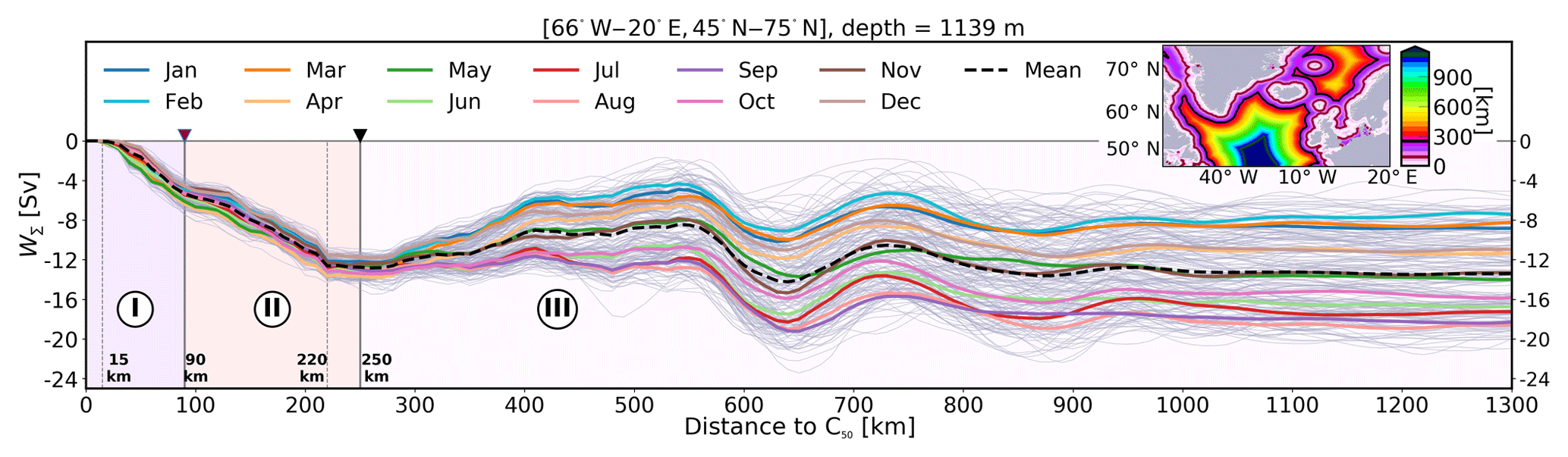
Figure 4Cumulative net vertical transport (W∑) at a depth of 1139 m (Sv) as a function of the distance from the bathymetric contour of 50 m depth referred to as C50 (inset map in Fig. 4). If the grid cell bathymetry is shallower no value is added. The dashed black line shows the annual mean. Monthly values of the 15-year simulation are shown in light gray, and colored lines indicate the monthly climatology. The regimes of sinking are indicated by roman numbers I–II–III, and the separation lines between them are also denoted by a brown and a black triangle as well as by contours in the same color in the inset figure.
- I.
-
Distance ≤ 90 km. This region presents the largest increase in sinking with respect to the distance to C50. It displays a small seasonal variation of less than 2 Sv. The minimum accumulated W∑ at 1139 m occurs in April (light orange line) and is around −6 Sv over a distance of ∼70 km.
- II.
-
Distance between 90 and 250 km. The accumulated W∑ in this section remains intense though smaller than in regime I with Sv over 130 km. The magnitude of accumulated W∑ increases until about 220 km from C50. Between 220 and 290 km the curve flattens, indicating that no additional sinking occurs or that it is locally compensated for by rising waters. Seasonal variations are slightly larger than for regime I, with values over 3 Sv between the months of April (light orange line) and December (light brown line).
- III.
-
Distance >250 km. Beyond 250 km from C50 the trend in accumulated W∑ can revert completely with respect to regimes I and II depending on the season. During winter months, there is a net positive accumulated W∑ (i.e., net upwelling) between 290 and 750 km; during summer months a negative accumulated W∑ tends to occur. As a result, the final amount of accumulated W∑ displays a large seasonal variability, with deviations of up to 11 Sv between winter and summer months at a distance of over 750 km from C50. The annual mean of accumulated W∑ varies little with distance from the coast in this regime (only 1−2 Sv; compare the black dashed line in Fig. 4 at 290 km and at 1000 km). The seasonal variations strongly affect the accumulated W∑ in some specific months (e.g., in February – light blue line – or in August – pink line), yielding changes in the accumulated W∑ of up to 50 % of what is seen in the first 290 km off C50.
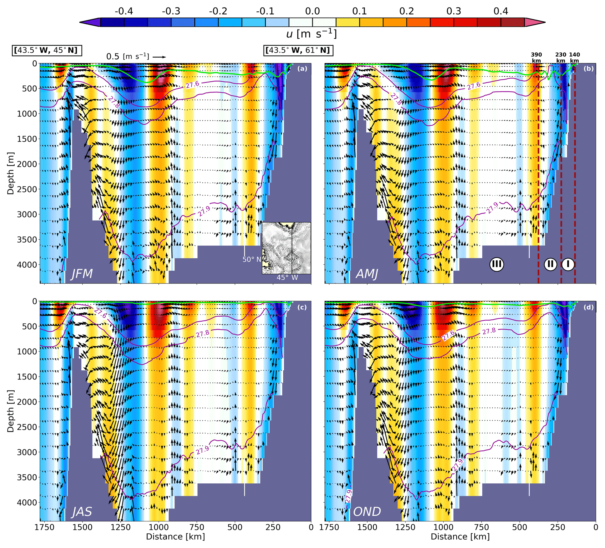
Figure 5The 15-year climatology of the velocity field at a cross section between the southern tip of Greenland and the southern limit of the study area (see inset in a; main surface currents denoted by black arrows). Each panel represents a seasonal average: (a) JFM (January–February–March); (b) AMJ (April–May–June); (c) JAS (July–August–September); OND (October–November–December). The shading shows the u component of velocity (m s−1); black arrows are velocity vectors constructed as (). For clarity arrows are shown for one of every three horizontal grid points at certain depths. The green line depicts the seasonal mean mixed layer depth (m), and the black contours denote the seasonal potential density anomaly, , for selected values. The limits of the proposed sinking regimes (I–II–III) are sketched in (b) by vertical dark red dashed lines.
It is hypothesized that these three sinking regimes reflect the effect of different processes contributing to the sinking. This is illustrated in Fig. 5 by means of a time-mean vertical cross section of the horizontal and vertical velocity field (see inset panel a). First, there is sinking of waters between 500 and 2000 m along the Greenland shelf slope all year round (black arrows on the right-hand of panels a–d). This sinking is connected with regimes I and II (Fig. 4), and occurs within the boundary current (blue shading) below the mixed layer depth (light green line). Most of this sinking is constrained to a distance around 200 km off C50 in a region where isopycnals are tilted and displays little seasonal variation. Second, there is a permanent anticyclonic eddy of about 200 km of diameter at 1000–1250 km south of the tip of Greenland that extends from the surface to a depth below 4000 m (shading) and generates both intense positive and negative vertical velocities at its flank (black arrows). This pattern of interior rising–sinking of waters yields a small net annual mean vertical transport over the entire basin but significant seasonal variability, which is reflected in sinking regime III (Fig. 4).
The boundary sinking found by Katsman et al. (2018) in a global ocean model and characterized here by regimes I and II is captured by the ageostrophic theory and in idealized models (Spall, 2010; Brüggemann and Katsman, 2019; Georgiou et al., 2019). Thus, the narrow band of sinking closer to C50 represented by sinking regime I is characterized by the preeminent role of topographically induced dissipation, while the sinking farther offshore represented by regime II is presumably largely driven by the presence of eddies near the boundary. Indeed, the amount of sinking is governed by eddy advection in the cross-shore direction (Georgiou et al., 2019), so it is not surprising that this region presents a larger seasonal signal compared to the one described by regime I (Fig. 4; see also the patches of strong EKE near the southern tip of Greenland in Fig. S5).
Spall and Pickart (2001) derived a simple expression to estimate the magnitude of meridional overturning (MB) – or by mass conservation, the downward vertical transport W∑ – near the boundary for a situation with a deep mixed layer:
where the amount of W∑ is proportional to the square of the mixed layer depth (h) and to alongshore differences in potential density (ΔρB), g is the Earth's surface gravity, f the Coriolis parameter, and ρ0 is a reference density. Although Eq. (2) is not formally correct when the mixed layer depth is shallow (as is the case here), Katsman et al. (2018) demonstrated that the relationship yields reasonable results in a realistic global ocean model when the mixed layer depth (h) is substituted by half the depth of the largest sinking and the alongshore density change (ΔρB, which for this situation depends on depth) by its depth average. Equation (2) indicates that the net vertical transport is, among other factors, controlled by the local alongshore density gradient (ΔρB), that is, a negative W∑ is associated with a rise in the isopycnals along the boundary current (or, equivalently, by the densification of waters at a given depth). This proportionality of the boundary sinking to the density gradient along the boundary was also pointed out by Straneo (2006) in her two-layer model approach. This connection is also suggested here by the strong vertical velocities in the boundaries (Fig. 2a, b) and by the upward displacement of the isopycnals between the eastern (southeast of Iceland) and the western (southwest of Greenland) sides of the basin (see the mean depth of isopycnals of σρ=27.75 and 27.8 kg m−3 in Fig. S6a, b). Indeed this alongshore tilting is always present and has its maximum in spring (Fig. S7).
Apart from the isopycnal tilting in the alongshore direction, Brüggemann and Katsman (2019) and Georgiou et al. (2019) found that the cross-shore density gradients also contribute to the budget of boundary sinking since, as eddies arise from baroclinic instabilities, they try to flatten the isopycnals. This can be accompanied by strong vertical velocities and hence more sinking (see, for example, the cross-shore density gradient in Fig. 5, where the isopycnal of σρ=27.8 kg m−3 is tilted within the boundary current near the southern tip of Greenland).
Finally, the sinking in regime III is related to those processes that develop away from the shelf and far from the core of the boundary current. In this case, strong vertical velocities appear at the edge of interior eddies, which are governed by different dynamics (Fig. 5). The major role of such quasi-permanent eddies is supported by the marked fluctuations between 300 and 1000 km in Fig. 4, the large interior eddy in Fig. 5, and the vigorous EKE field in the interior of the Newfoundland Basin near the Flemish Cap (Figs. S4 and S5).
The overall view of net vertical transport (W∑) in the subpolar North Atlantic presented in the Sect. 3 may not be valid at regional scales, since the bathymetric configuration, the ocean circulation, and water-mass properties differ between the different seas. Moreover, the dynamics of overflows are different from those governing the near-boundary sinking induced by the buoyancy loss of a boundary current. In order to assess and understand these expected spatial variations we divide the subpolar North Atlantic in eight well-established regions (see Fig. 6), which for discussion purposes can be grouped into three more general sets: marginal seas (Labrador, Irminger, Greenland, and Norwegian seas; Sect. 4.1), overflow regions (Denmark Strait and Iceland–Scotland Ridge; Sect. 4.2), and midlatitude seas (Newfoundland and Rockall; Sect. 4.3). In the remainder of this section we will describe the following properties associated with W∑ for these three groups of regions:
- I.
the time-mean W∑ at the depth of minimum W∑ (hereinafter this depth is defined as zmin);
- II.
the seasonal variability of W∑ and zmin;
- III.
the signal-to-noise ratio (SNR), defined as (μ= time mean of W∑ at zmin, σ= standard deviation of W∑ at zmin; a high value (SNR>1) indicates that μ is relatively large compared to σ, whereas a small value (SNR<1) denotes a signal with a large temporal variability compared to the mean, although it does not necessarily imply a well-defined seasonal signal as SNR does not yield any information on its periodicity); and
- IV.
the regimes of sinking that can be identified.
In Sect. 4.4, a further evaluation of the sinking characteristics of the Labrador Sea, Irminger Sea, and Newfoundland regions (which represent about 2∕3 of net sinking in the subpolar North Atlantic and cover all three types of regions) is provided.
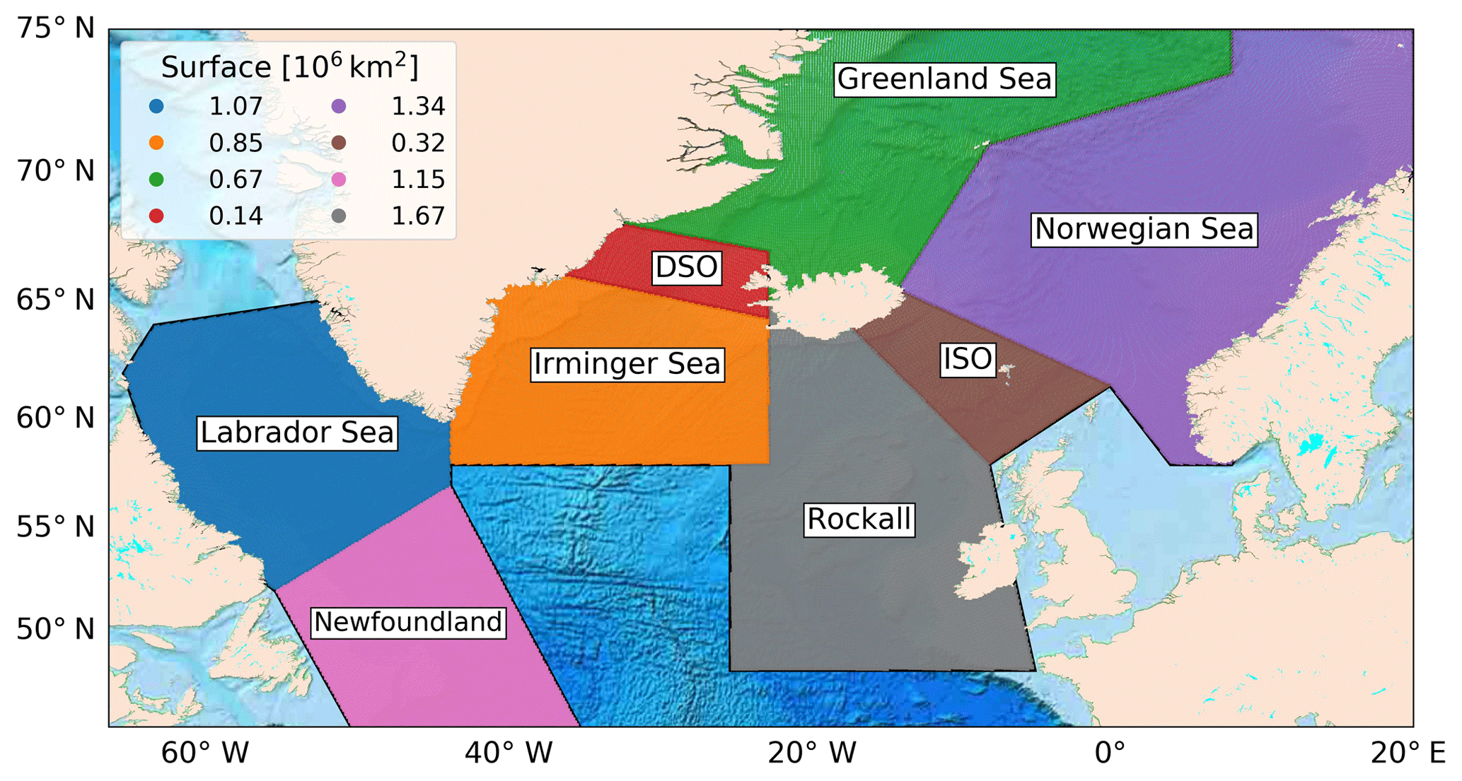
Figure 6Map of the North Atlantic (66∘ W–20∘ E, 45–75∘ N) divided into eight regions. DSO and ISO refer to the Denmark Strait and Iceland–Scotland Ridge overflow regions, respectively. The surface area of each region is shown in the legend (106 km2).
4.1 Marginal seas
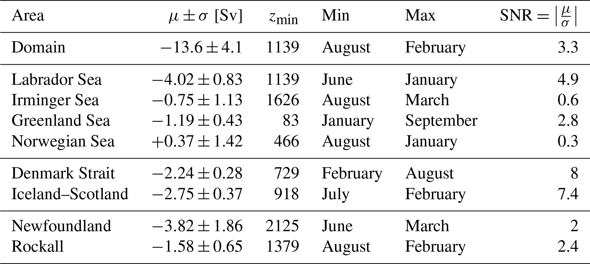
Vertical profiles of W∑ for the marginal seas (Fig. 7a–d) indicate that on average the Labrador Sea contributes about twice as much to the sinking as the other three marginal seas combined (−4.02 Sv against −1.57 Sv), yielding a total mean W∑ of −5.59 Sv in the marginal seas (see μ in Fig. 7a–d and Table 2 for a complete summary; notice the different value of zmin for each region). This contribution from the Labrador Sea is larger than the −1.4 Sv derived by Katsman et al. (2018) using a coarser ocean model (ORCA025). This is probably due to the improved ability of higher-resolution models to resolve the eddy activity and ageostrophic processes near the boundary (Georgiou et al., 2019; Brüggemann and Katsman, 2019), which gives rise to stronger vertical transports. It is also larger than the −1 Sv estimated by Pickart and Spall (2007) using the World Ocean Circulation Experiment (WOCE) AR7W line data and the −1.2 Sv estimated from Argo floats by Holte and Straneo (2017) at a shallower depth (around 800 m). This substantial difference may be due to the scarcity of observations. Interestingly, the value of zmin for the Labrador Sea matches the one previously shown in Fig. 3a for the whole basin (1139 m). The Greenland Sea also shows a time-mean W∑ that stays negative during the whole year of about −1.2 Sv (Fig. 7c), with the minimum W∑ (largest sinking) occurring in June and the maximum in February (Table 2). In this case zmin is located at a depth around 80 m, with a quasi-linear decrease in the magnitude of sinking until a depth of 1800 m at which it is nil. The sinking in the Irminger and Norwegian seas is more variable and depends on the time of the season, yielding net positive (negative) W∑ during winter (summer) months (Fig. 7b, d). This yields a smaller annual mean sinking than in the Labrador and Greenland seas for the Irminger Sea of −0.75 Sv and net upwelling of +0.37 Sv for the Norwegian Sea. A notable difference between the Irminger and Norwegian seas is the value of zmin, which is ∼470 m for the Norwegian Sea and ∼1630 m for the Irminger Sea.
Table 2Summary of properties of the sinking shown in Figs. 3a and 7 for the entire study area (“Domain”) and all regions defined in Fig. 6; μ denotes the time-mean net vertical transport (W∑) at the depth of minimum W∑ (zmin), and σ is its the standard deviation. “Min” and “Max” denote the months when the minimum and maximum W∑ (or equivalently the largest and the smallest sinking) occur, respectively. The final column shows the signal-to-noise ratio (SNR), defined as .
The magnitude of the seasonal variability of W∑ is exhibited in Fig. 8, where the time series of W∑ at zmin with (solid lines) and without (dashed lines) the seasonal signal are depicted for each region (Fig. 7 and Table 2). It displays a negative W∑ all year round for the Labrador Sea that varies between −2 Sv (winter) and −5 Sv (late spring–summer). This result for the Labrador Sea agrees qualitatively with Holte and Straneo (2017), who also found the strongest sinking in spring (−1.2 Sv) and the weakest sinking in winter (−0.6 Sv). Georgiou et al. (2019) also found this intensification of the sinking during spring in their idealized Labrador Sea model in response to the larger density gradients between the boundary and the interior. The Irminger and Norwegian seas share a large temporal variability that is reflected in an elevated standard deviation of ∼1.1 and 1.4 Sv, respectively (Fig. 7b, d), and a seasonal variability of ∼3 Sv, similar to that found in the Labrador Sea (Fig. S8b, d). For the Irminger Sea, zmin remains constant during the year, while for the Norwegian Sea it changes every season with an abrupt deepening in winter when it reaches a depth of ∼1200 m (horizontal dashed black lines in Fig. S8b, d). The Greenland Sea also shows some seasonal variability of W∑ at zmin (1 Sv; Fig. S8c), with the depth of largest sinking shallowing significantly during winter to ∼100 m (black dashed lines in Fig. 7c) when the strongest sinking occurs. In terms of SNR, the Labrador Sea has a high value of ∼4.8, which is larger than for the Greenland Sea (2.8). In contrast, the Irminger and Norwegian seas yield low values of SNR (0.7 and 0.25, respectively; Table 2), which reflect their remarkable seasonal variability (Fig. S8b, d). The boundary sinking is delayed from the occurrence of deep convection in the interior of the subpolar North Atlantic as demonstrated by the fact that the largest boundary sinking in the Labrador and Irminger seas occurs in late spring–summer, while the deep convection takes place in late winter–early spring (Fig. S2).
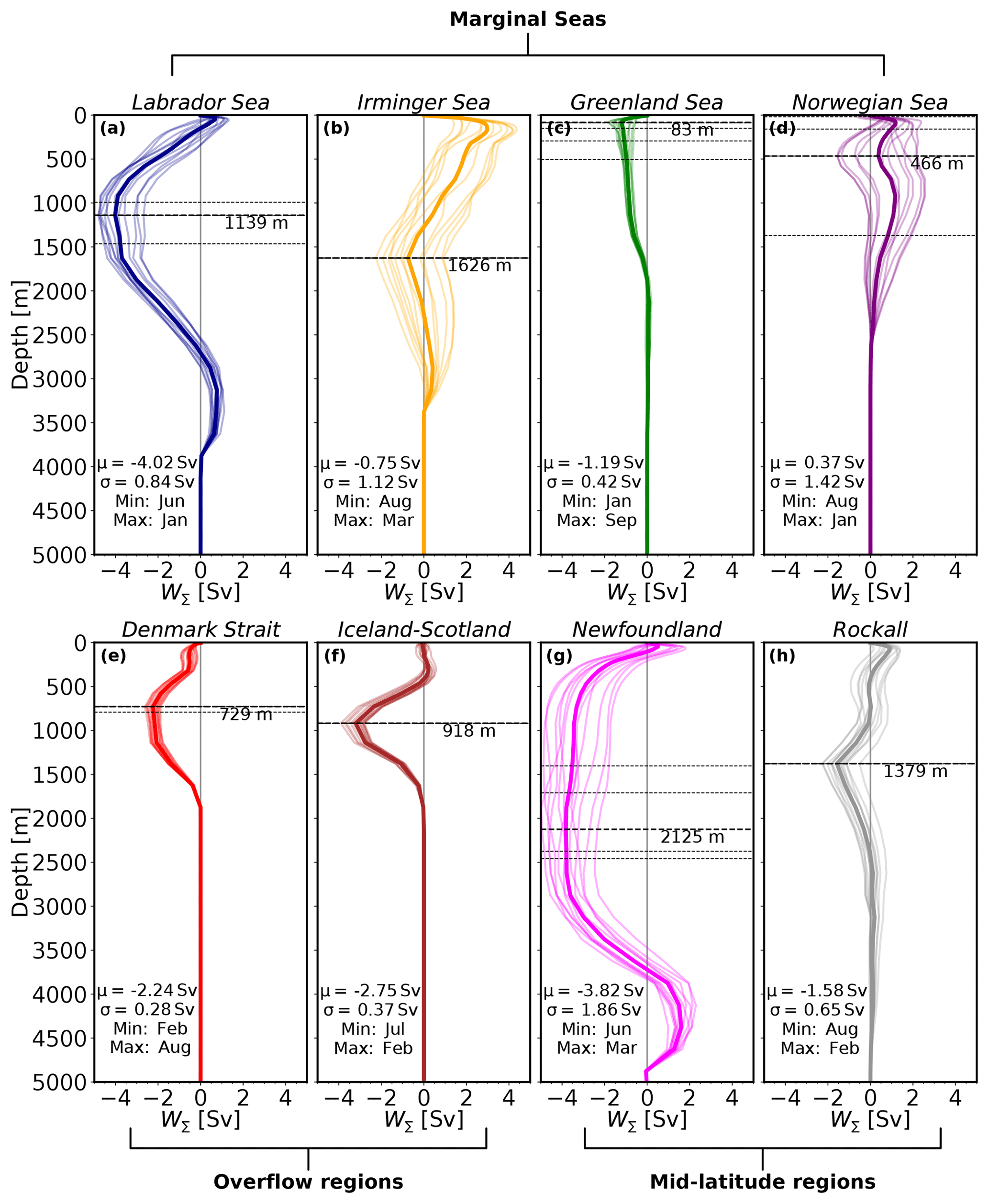
Figure 7Vertical profile of annual mean (thicker line) and monthly averages (thinner lines) of net vertical transport (W∑) for the regions defined in Fig. 6; μ and σ are the climatological mean and standard deviation of W∑ at the depth of largest sinking (or minimum W∑; see legend). zmin is the depth at which the largest sinking is found. “Max” and “Min” refer to the months with maximum and minimum mean W∑ (smallest and largest sinking), respectively. Seasonal mean depths of W∑ are displayed as horizontal black dashed lines.
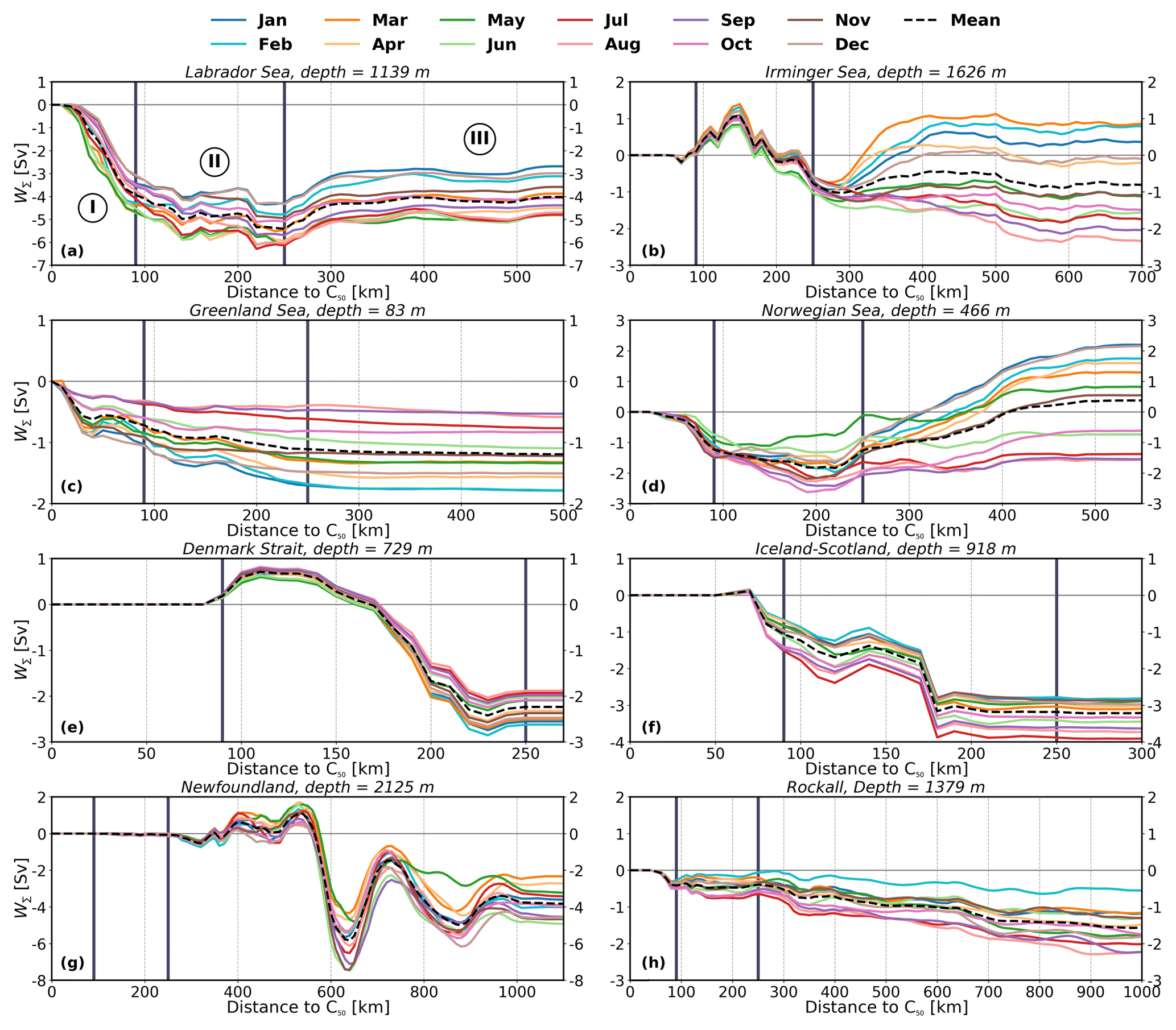
Figure 8Accumulated net vertical transport (W∑) with respect to the distance to the closest bathymetric contour of 50 m (C50). Distances are shown in Fig. 4 (inset map). Annual (dashed black line) and monthly mean (colored lines) curves are depicted for the regions defined in Fig. 6. The accumulated W∑ has been calculated at the depth of minimum time-mean W∑ (zmin), which differs for each region (see Table 2 and plot title). The bounds separating the sinking regimes (I–II–III) proposed in Fig. 4 (90, 250 km) are indicated with thicker solid vertical lines. Note the differences in the horizontal and vertical scales in the plots.
Next, we evaluate to what extent the sinking regimes proposed in Sect. 3.2 for the entire subpolar North Atlantic are also applicable to the individual regions of interest. To this end we have plotted the accumulated W∑ from C50 to the interior at the depth of largest sinking for each region (Fig. 8). Overall, the Labrador, Greenland, and Norwegian seas show the sinking regimes proposed in the Sect. 3.2, with a stronger negative accumulated W∑ near the slope at distances shorter to C50 than 200 km and a small accumulated W∑ at larger distances. In particular, the Labrador Sea yields an accumulated sinking W∑ of around −4 Sv in the region covered by sinking regime I, which is larger in magnitude than the −1 Sv and the −0.5 Sv obtained for the Norwegian and Greenland seas, respectively, for the same region (Fig. 8a ,c, d). The amount of negative accumulated W∑ in regime II is generally smaller in magnitude in the individual regions: roughly −1.5 Sv for the Labrador Sea, −0.5 Sv for the Greenland Sea, and 0 Sv for the Norwegian Sea (Fig. 8a, c, d). Differences between sinking regimes I and II are subtle but still distinguishable, such as the slightly larger seasonal variability (up to 2 Sv for the Labrador and Norwegian seas) and the higher number of oscillations at distances within regime II. In contrast, the Irminger Sea shows a succession of positive–negative accumulated W∑ over the distances covered by regimes I–II, with a negative accumulated W∑ at 250 km of around −1 Sv. Depending on the marginal sea considered regime III is found 200–300 km off C50 (shorter for the Greenland Sea due to its shallower depth of largest sinking), and it is associated with larger monthly variations of accumulated W∑ than in regimes I and II. Some clear examples of this seasonality are exhibited by the Irminger, Norwegian, and Labrador seas with ranges ∼2–3 Sv (Fig. 8a, b, d); the Greenland Sea also shows a clear seasonality but weaker (1 Sv), in line with Figs. 8c and S8c. We note that the pattern of accumulated W∑ is particularly complex for the Irminger Sea on and near the slope, with positive accumulated W∑ at a distance to C50 between 90 and 150 km followed by negative accumulated W∑ between 210 and 300 km off C50. One explanation for that succession of upward–downward moving waters near the boundaries is the uphill–downhill flow along the coast, which is probably linked to the bathymetry (as seen in Fig. 2a and also supported by a depth of largest sinking that does not vary seasonally in Fig. 7 and by a more dedicated assessment of W in Fig. S9). At distances of more than 300 km from C50, the Norwegian and Irminger seas show a positive accumulated W∑ during winter, yielding a seasonal variation with respect to summer months of 3 Sv. To summarize, our results confirm that to a large extent the proposed sinking regimes remain applicable to marginal seas, in particular to the Labrador Sea. However, the mentioned differences and similarities among the marginal seas (e.g., their different zmin) reveal a complex picture, whereby the boundaries between the different regimes are not fixed and can shift a few tens of kilometers closer to or farther from C50. That is, sinking regimes are influenced by the local bathymetric features and processes in each marginal sea.
4.2 Overflow regions
The Denmark Strait and the Iceland–Scotland Ridge are regions where W∑ is mainly dominated by the overflow of waters from the Nordic Seas towards the northern subpolar North Atlantic. Figure 7e–f show that the mean magnitude of W∑ is very similar in both regions and amounts to roughly −2.2 and −2.7 Sv in the Denmark Strait and Iceland–Scotland, respectively. Altogether it gives a total value of Sv for overflow waters, which represents at most 37 % of the total W∑ at zmin (compare overflow regions against the domain in Table 2). The outcome from the Denmark Strait is in agreement with the −2.2 Sv estimated by Katsman et al. (2018) for the ORCA025 hindcast (note that they estimated W∑ in a different area and zmin) and 0.25 Sv higher than the transport found by Köhl et al. (2007) in a model simulation. However, these model-based results are about 1 Sv weaker than the hourly observations, which yield Sv (Jochumsen et al., 2017). zmin differs for both regions and is shallower for the Denmark Strait (729 m) than for Iceland–Scotland (918 m). This is related to the respective sill depths in the model.
The downward transport in the Denmark Strait peaks in February and is weakest in July, which is out of phase with all other regions; the Iceland–Scotland region peaks in July and is weakest in January (Table 2). Seasonal variability is present in both time series with ranges of 0.6 Sv for the Denmark Strait and 1 Sv for Iceland–Scotland (which is poorly defined in some specific years) at their respective zmin (solid lines in Fig. S8e–f and Table 2). This depth also shows larger seasonal variations in Iceland–Scotland than in the Denmark Strait (black horizontal dashed lines in Fig. 7e–f). The seasonal signal is smaller in the Denmark Strait than in other basins, with differences between winter and summer (Fig. S8e) likely due to fluctuations of the overflow plume (Jochumsen et al., 2017; Håvik et al., 2017), which has an observed reduced transport in summer. As with other high-resolution models, this model simulation tends to overestimate seasonal changes in overflow waters through the Denmark Strait: observations indicate a seasonal signal of only around 0.05 Sv (Jochumsen et al., 2012). Moreover, sinking in Iceland–Scotland displays slightly larger fluctuations than in the Denmark Strait (SNR=7.4 against SNR=8). This can be explained by its larger extent, which in this case covers two sills: one near Iceland and another closer to Scotland.
More differences between the Denmark Strait and the Iceland–Scotland regions become apparent from Fig. 8e–f where the time-mean accumulated W∑ is plotted versus the distance to C50. The positive and negative accumulated W∑ in the Denmark Strait over the first 250 km off C50 (Fig. 8e) reflect waters moving southward from the Nordic Seas that first flow up and then down over the sill. This is illustrated by the deepening of the isopycnal in Fig. S6c after crossing the Denmark Strait and demonstrated in Fig. 9, in which the Denmark Strait region has been divided in two parts of similar size on either side of the sill (green triangle in Fig. 9a): one that mainly contains the upward movement of waters as they approach the sill (DSO ↑) and another that contains the downward movement of waters after crossing the sill (DSO ↓). As a result, this up–down transport is clearly reflected in Fig. 9b–c, with the strongest upwelling (+1 Sv) located at a depth of 579 m, and the strongest sinking (−3 Sv) is found at 729 m. The difference between DSO ↑ and DSO ↓ accounts for the near 2 Sv of net sinking found in this region. Furthermore, the accumulated vertical transport with respect to the distance to the sill at the respective depths of strongest upwelling and sinking show that the most important contributions occur within the first 150 km off the sill.

Figure 9(a) Map of Denmark Strait overflow region (DSO). The mean vertical transport (W) at 729 m is depicted by shading (color). The triangle illustrates the location of the sill (green triangle) that separates the Denmark Strait in two areas of similar size (DSO ↑ and DSO ↓). Bathymetric contours are indicated by a black line. (b, c) Vertical structure of transport (W∑) in DSO ↑ and DSO ↓, respectively. (d) Annual (dashed line) and monthly (red solid lines) accumulated vertical transport with respect to the sill in DSO ↑ (red) and in DSO ↓ (light blue ). Both have been calculated at the corresponding depths of largest upwelling (579 m) and sinking (729 m) for DSO ↑ and DSO ↓, respectively.
In Iceland–Scotland the strongest sinking can be identified for distances to C50 smaller than 100 km but relatively far when compared with the Labrador and Norwegian seas. Sinking is larger in summer than in winter. The two sills are clearly identifiable in Fig. 8f: the first near Scotland at around 80 km and the second near Iceland at about 180 km from C50. So our results indicate that the classification in sinking regimes does not capture some specific features of the overflows. This is not surprising, since they are governed by different dynamics. Indeed, the location where sinking associated with overflows occurs is not determined by lateral boundaries but rather by the bathymetry, so it can occur at distances to the shelf distinct from the pattern shown by the marginal seas.
4.3 Midlatitude seas
Finally, we discuss the characteristics of the vertical transport in two regions at midlatitudes: Newfoundland, located further south in the vicinity of the Gulf Stream, and Rockall, which occupies the east Atlantic between 25∘ W and 5∘ E of Iceland. Together they yield a time-mean W∑ contribution of Sv at zmin (Fig. 7g, h). Newfoundland is the region with the second largest W∑ after the Labrador Sea, with a sinking of −3.8 Sv. About −0.5 Sv of the sinking contained in Rockall takes place near the south of Iceland. A significant difference between the two regions is zmin, which is much deeper in Newfoundland (2125 m) than in Rockall (1379 m). Indeed, sinking extends deeper in Newfoundland, even reaching depths below 3000 m (Fig. 7g). The minimum (maximum) W∑ at zmin occurs in summer (winter) for both areas: in June (March) and August (February) for Newfoundland and Rockall, respectively. Although monthly variations reach 4 Sv for Newfoundland and 2 Sv for Rockall (solid curves in Fig. S8g, h), the seasonal cycle is not very pronounced for either of the two regions at zmin, although it is clearer for Rockall. The much larger temporal variability for Newfoundland is reflected in σ=1.86 Sv against the σ=0.65 Sv of Rockall, despite the SNR being rather similar (2 against 2.4).
Clear differences are seen when we compare the accumulated W∑ with respect to the distance to C50 (Fig. 8g–h for the two regions). Interestingly, Newfoundland displays large oscillations of positive and negative accumulated W∑ with wavelengths of about 200 km. This suggests the presence of permanent mesoscale eddies in the ocean interior, which are able to induce such strong vertical velocities, as shown in Fig. 5. In contrast, Rockall shows on average a quasi-linear decrease in the mean accumulated W∑ with respect to the distance to C50 that is more intense in the area within regime I. It also displays seasonal variability that, for example, yields a smaller sinking during late winter and spring months. We conclude that mean features of sinking in the Newfoundland and Rockall regions show similar characteristics to those seen for the entire subpolar North Atlantic, as reflected by some boundary sinking in Rockall (regime I) and the strong vertical velocities at large, semipermanent eddies likely detached from the North Atlantic Current in the interior of Newfoundland (regime III).
4.4 Further characterization of sinking regimes illustrated by selected regions
In this section we discuss in more detail the differences in sinking based on three regions: the Labrador and Irminger seas and Newfoundland. These regions represent around 2∕3 of the total sinking, are relatively far from overflows (although some contribution may be expected in the northern Irminger Sea), and present remarkable differences in their dominant sinking regimes covering a wide range of patterns that can be identified in other marginal seas as well. The spatial distribution of time-mean vertical transport (W) for the three regions at the corresponding depth of largest sinking (zmin), which differs for each region according to Table 2, is shown in Fig. 10a; the difference between the W calculated during the months of minimum and maximum W∑ is shown in Fig. 10b (these months, distinct for each region, are also indicated in Table 2). We have added black contours to illustrate the positive–negative variation of the climatological mean EKE between the respective months at zmin (Fig. 10b).
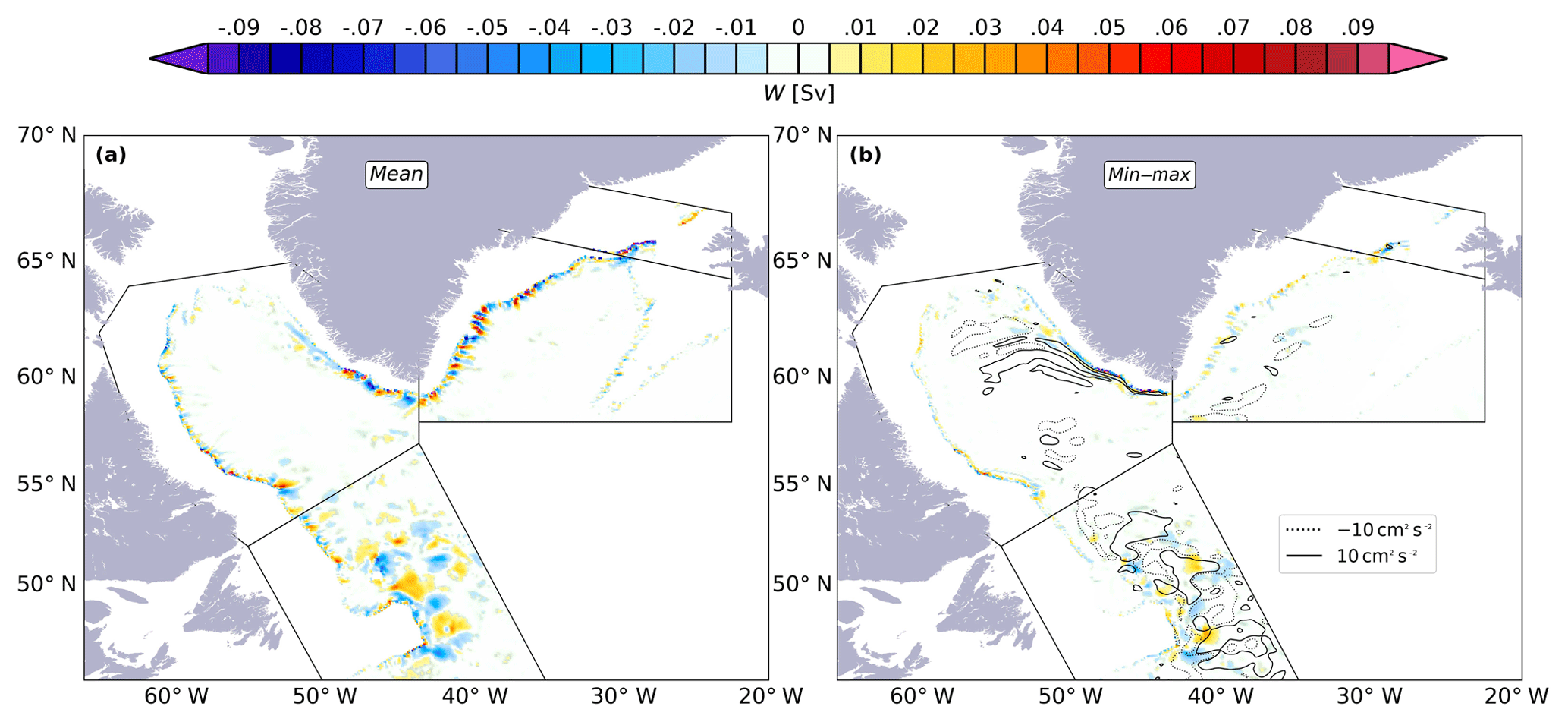
Figure 10(a) Composite map of mean vertical transport (W) for the western regions of study (defined in Fig. 6) at the corresponding depth of minimum time-mean W∑, which differs for each region according to Table 2. (b) Same as (a) but now the mean W (shading) and EKE (blacks contours; see legend) in the month of minimum W∑ minus the mean W in the month of maximum W∑ are plotted. These months of minimum and maximum sinking also change for each region according to Table 2 (W: Sv, EKE: cm2 s−2).
The Labrador Sea, which yields the largest contribution to the time-mean W∑, is the most representative sea where all the necessary ingredients for boundary sinking are fulfilled: a cyclonic boundary current, strong alongshore and cross-shore density gradients, a steep bathymetric slope, and an active eddy field (Brüggemann and Katsman, 2019; Georgiou et al., 2019). As a result, the three sinking regimes proposed for the entire subpolar North Atlantic in Fig. 4 were also identified in Fig. 10a for the Labrador Sea. The strong W near the boundary in the Labrador Sea (Fig. 10a) intensifies at the western side of the southern tip of Greenland during late spring, which is associated with a nearby increase in EKE (see the solid black contours over the blue patches in Fig. 10b and the patches of EKE in Fig. S5c–e around the tip). Indeed, the Labrador Sea displays an increase in the average horizontal speed of the boundary current at zmin during late winter and spring (Fig. 11a), which may enhance the horizontal velocity shear. As a result, we can expect an increase in the mean advection of vorticity between the coast and near the peak of the boundary current (at around 70 km off C50, mostly within the region covered by regime I; Fig. 11a) and a decrease offshore of the location of the maximum speed (with a part within the regime II) that may be compensated for by the presence of more eddies. The more active role of eddies exchanging waters between the interior and the boundary agrees with the reduced cross-shore potential density gradients found in regions I and II (green and orange lines in Fig. 11b). The idea that changes in EKE pathways may facilitate the intensification of sinking is further discussed by Georgiou et al. (2019) for an idealized convective basin mimicking the Labrador Sea.
In contrast to the Labrador Sea, the change in W in the Irminger Sea between the months of minimum and maximum time-mean W∑ is significantly smaller (Fig. 10b). This finding, together with the permanent depth of largest sinking (zmin) and the up and down distribution of sinking found in Fig. 8b, supports the hypothesis that the sinking near the boundary in the Irminger Sea is mostly quasi-stationary and topographically driven (see a detailed example of this up–down of waters in Fig. S9), which explains the small amount of net sinking found. In Fig. 8b it can be observed that there is a large difference (in terms of seasonal variability) between the sinking regimes I–II and the regime III in the Irminger Sea, which is probably driven by interior eddies. An interesting point to mention is the stronger mixing of waters within regions of regimes I–II (or, equivalently, the reduction of the cross-shore gradient) during the months of late winter and spring (orange and green lines in Fig. 11d). This pattern reflects a different behavior from what we find in the Labrador Sea or Newfoundland (Fig. 11b, f) and is accompanied by an intensification of the boundary current during the same months (orange and green lines in Fig. 11c). This difference is also reflected in the positive vertical transport during winter within regime II (blue and orange lines in Fig. 8b) and reinforces the crucial importance of topographic features in driving the boundary sinking in the Irminger Sea.
Newfoundland yields the second largest contribution to sinking, which is largely produced within sinking regime III. The strong seasonal variations of W in the Newfoundland region below 2000 m are mostly related to EKE interior pathway changes (see black contours in Fig. 10b) impinged by North Atlantic Current fluctuations and meandering. The fact that strong vertical velocities appear at the edge of large eddies in the interior, thus contributing to upwelling–sinking, has been already shown in Figs. 9g, 10a–b, and S4, where a train of large eddies near the Flemish Cap is visible. Finally, in the Newfoundland region the peak of the boundary current at its corresponding zmin falls in regime III (Fig. 11e); although the strongest sinking occurs in the interior and below 2000 m, there is some sinking at shallower depths as indicated by its vertical structure in Fig. 7g (Fig. S4). Similar plots showing the overall weaker spatial patterns of sinking for the remainder of the regions can be found in Figs. S10 and S11.
In Sect. 3 we demonstrated the consistency between the overturning streamfunction (ψo) at the southern boundary of our study area at 45∘ N and the total net vertical transport (W∑) in the subpolar Atlantic basin (Fig. 3b). As the amount of accumulated negative W∑ appeared to differ between the boundaries and the interior, we have classified the sinking according to three regimes (Fig. 4). Moreover, in Sect. 4 we have evaluated the spatial patterns and the seasonal variability of sinking at the regional level. The fact that nearby areas exhibit striking differences in the amount, seasonality, and distribution of W∑ suggests that, to a large extent, it depends on local dynamics and bathymetry. However, it still remains unclear how regional boundary sinking is related to the AMOC strength. For instance, does a decrease–increase in Labrador Sea W∑ have any quantifiable effect on the AMOC? To address this we have computed the cross-correlation between the reverted time series of the maximum of ψo at 45∘ N (red lines in Fig. 3b) and the time series of W∑ (Fig. 8) for each region at the depth of largest sinking (zmin; Table 2). We have performed the analysis for two cases: with seasonal variability (Fig. 12b) and without seasonal variability (Fig. 12c). Figure 12a shows the monthly climatology of sinking at their corresponding zmin so that the months with the largest and smallest sinking for all regions (Table 2) are easily identifiable. Solid lines in Figs. 3b and 9 include the seasonal signal, whereas the dashed lines indicate that seasonality has been subtracted. A positive correlation at a positive time lag τ means that stronger (weaker) sinking yields a stronger (weaker) AMOC (ψo) at 45∘ N τ months later.

Figure 11The 15-year climatology of the following variables with respect to the distance to the coast (according to the inset map in Fig. 4) for (a, b) the Labrador Sea, (c, d) the Irminger Sea, and (e, f) Newfoundland: (a, c, e) horizontal speed of current at the depth of largest sinking (zmin, Table 2); (b, d, f) potential density anomalies (; kg m−3) averaged between z layers 14 and 24 (∼220–1650 m). For all panels the dashed black line depicts the mean, whereas colored lines show the monthly average. The bounds between the sinking regimes proposed in Fig. 4 are indicated with thicker solid vertical lines. Note the differences in horizontal scales of the subpanels.
The high correlation between W∑ for the entire subpolar North Atlantic (DOMAIN) and ψo (>0.9; mentioned in Sect. 3) appears clearly at zero lag for both study cases. The time lags found for regions are also in agreement with the temporal separation between the corresponding months of minimum W∑ and the month of maximum ψo at 45∘ N. For instance, the Labrador Sea displays the minimum sinking in June, whereas ψo has its maximum in August (Fig. 12a). As a consequence, the highest correlation is found for a lag of the AMOC of 1–2 months. The same is found for all other regimes, including the Denmark Strait, which has the minimum W∑ in February, yielding a negative correlation at zero lag. Figure 12b shows that for the southern regions (Rockall and Newfoundland) correlations are surprisingly weak. One reason for this is that the signal of negative W∑ is very noisy for these two regions, with no clear seasonal cycle (Fig. S8g–h), while ψo has a clear seasonal signature. For the Greenland Sea correlations are also rather weak (<0.4), presumably due to its small seasonal variability (Fig. S8c).
To eliminate the influence of seasonality we repeat the analysis on the deseasoned signal. Resulting correlations (Fig. 12c) demonstrate that the only region with a significant correlation between variations of sinking and ψo is Newfoundland. This is the region with the largest non-seasonal variations (Fig. S8g, dashed line) and that shares its boundary with ψo at 45∘ N. Therefore, it is reasonable to think that any change in the North Atlantic Current, either in strength or position, will be reflected in sinking in Newfoundland and vice versa (for instance, a fluctuation in the train of eddies in the interior of the Newfoundland region).
The existence of a high correlation does not necessarily imply that variations in the sinking waters govern the AMOC, as the different regions in this simulation are subject to the same strong large-scale forcing, for instance the seasonal heat fluxes or wind stress variations that affect middle and high North Atlantic latitudes. Thus, the AMOC and the sinking are likely responding synchronously to variations in large-scale forcing. Therefore, our results using an Eulerian standpoint do not evidence that a variation (marked increase–decrease) in W∑ at any of the marginal seas propagates to the lower cell of the AMOC. To investigate this in more detail requires the use of a Lagrangian approach to track the boundary sinking and subsequent spreading of waters, which is beyond the scope of this paper.
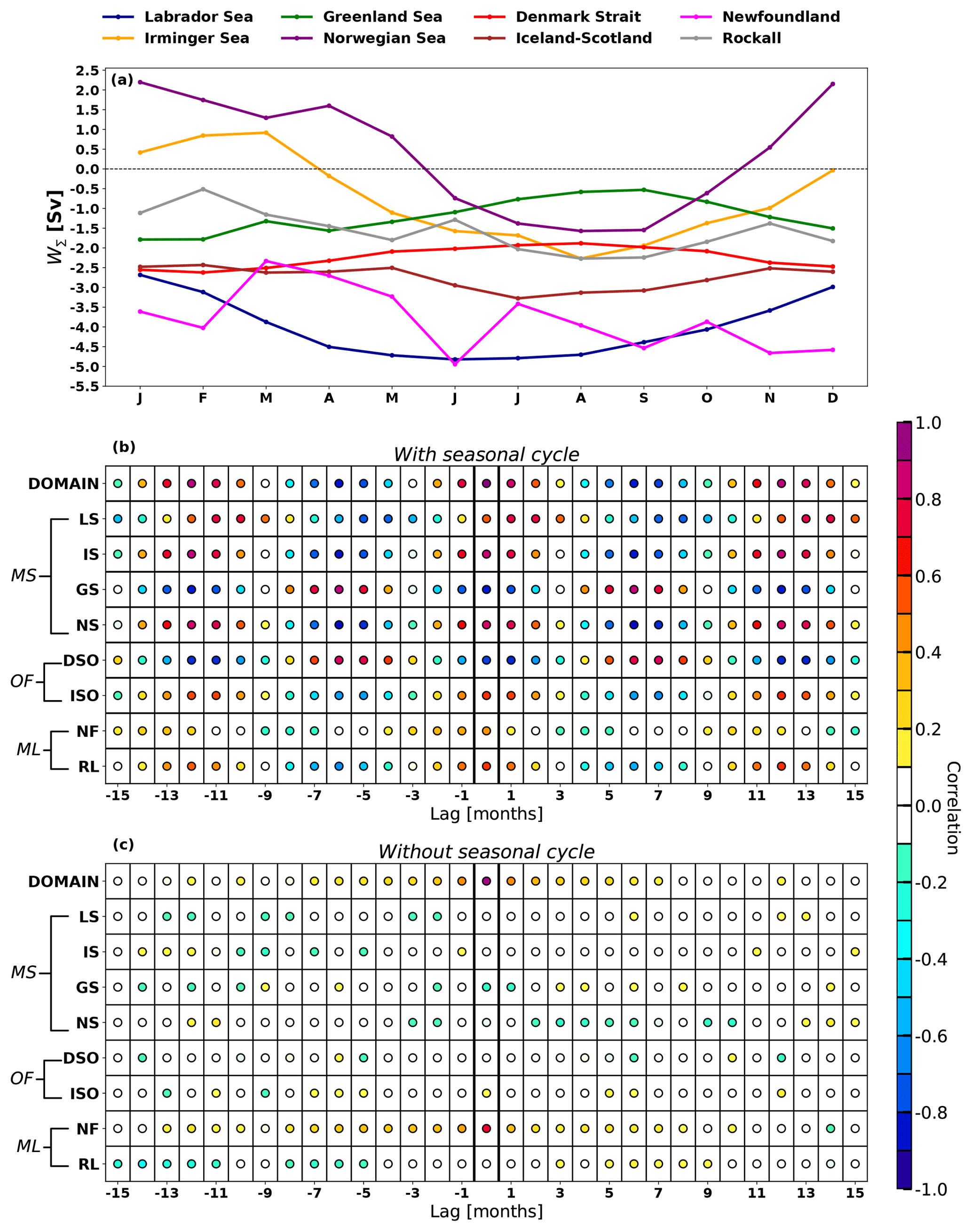
Figure 12(a) Time series of the monthly climatology of W∑ for the regions defined in Fig. 6 at the depth of largest mean sinking (zmin, which differs between regions according to Table 2). (b) Cross-correlation between the maximum of the reverted overturning streamfunction (ψ0) at 45∘ N (red lines in Fig. 3b) and the regional time series of net vertical transport, W∑ (Fig. S8), at the depth of minimum time-mean sinking for a set of time lags (in months). (c) As (b) but without the seasonal variability. The seasonality has been removed by subtracting the corresponding 15-year monthly mean (i.e., a for the regional time series). Sinking leads over ψ0 for positive lags. DOMAIN refers to the whole study area (Fig. 6) and the acronyms are defined as Labrador Sea (LS), Irminger Sea (IS), Greenland Sea (GS), Norwegian Sea (NS), Denmark Strait overflow (DSO), Iceland–Scotland Ridge overflow (ISO), Newfoundland (NF) and Rockall (RL), marginal seas (MS), overflow regions (OF), and midlatitude seas (ML).
Based on a high-resolution ocean model simulation forced by a prescribed annual cycle of wind, precipitation, and heat fluxes, we have found that the amount of minimum time-mean net vertical transport (W∑) for the entire subpolar North Atlantic Ocean is consistent with the transport and vertical structure of the AMOC core at midlatitudes (45∘ N), with an average of about −14 Sv at a depth of 1139 m. Moreover, the prescribed annual cycle introduces a strong seasonality that favors more sinking of waters at basin scale and a stronger AMOC during summer than in winter, with a similar seasonal variability in both signals (∼10 Sv). However, this picture becomes much more complex at regional scales, as is illustrated by the different depths at which the largest sinking occurs (ranging from 460 to 2000 m), the distinct spatial distribution, and the asynchronous seasonal variations of W∑ that are found for the different regions in the subpolar North Atlantic.
In accordance with recent studies, our model results confirm that the largest vertical transports occur near the boundaries below the mixed layer depth (Katsman et al., 2018; Brüggemann and Katsman, 2019; Georgiou et al., 2019), in a narrow band that extends between 50 and 250 km off the contour of 50 m of depth (C50). When we consider the sinking over the whole subpolar North Atlantic, three dominant sinking regimes are revealed: regime I (∼0–90 km) appears where the topographic dissipation is largest, regime II (∼90–250 km) covers the remainder of the continental slope, and regime III (distances >250 km) occurs in the ocean interior. Our results indicate that around 90 % of the accumulated sinking takes place in the area covered by regions I and II, while the largest seasonal variability of sinking occurs in region III. The near-boundary sinking in regimes I and II is thought to be governed by the ageostrophic dynamics discussed by, e.g., Spall and Pickart (2001) and Straneo (2006), and its amount depends on the interplay of several factors: the existence of a boundary current, a steep slope, the presence of eddies, and the alongshore and cross-shore density gradients (sloping isopycnals). This implies that the budget of W∑ is potentially sensitive to the intensity and the width of the boundary current, the strength of the eddy field, and the dominant eddy paths (Georgiou et al., 2019).
Distinguishing by regions, we find that most sinking occurs in the Labrador Sea ( Sv), Newfoundland ( Sv), and the overflow regions (Denmark Strait and Iceland–Scotland Ridge with Sv altogether). The Irminger and Norwegian seas show a strong seasonally dependent behavior, with sinking during part of the year, upwelling the rest of the year, and hence little net sinking. We identified the three sinking regimes in almost all regions except in the overflow regions, which are governed by different dynamics, and in the Irminger Sea. The Irminger Sea shows distinct sinking dynamics near the boundary due to the existence of bathymetry-forced flows and probably by some overflow waters coming from the Denmark Strait. Moreover, in each region the distance from the coast that marks the boundary between the sinking regimes is seen to shift due to the local dynamics and bathymetric features (e.g., different steepness or shelf width) of each region.
The dominance of the seasonal forcing in the sinking response (probably induced by the repeated forcing conditions) prevents us from finding a connection between the regional variations of sinking and the lower cell of the AMOC at midlatitudes, though previous research has suggested a complex interaction between the surface atmospheric forcing, the boundary current, and interior waters for which eddies play a crucial role (Georgiou et al., 2019). To gain insight into this connection would require an analysis of the near-boundary sinking and the AMOC in a model simulation with varying surface forcing. In addition, we have studied the Eulerian net vertical transport without referring to the water-mass properties, while the subpolar North Atlantic is characterized by a strong densification of waters during late winter and spring. The latter would require an assessment of sinking in density space; this is outside the main scope of this study, which focuses only on the vertical structure, seasonality, and spatial distribution of sinking. Also, we note that monthly fields allow us to accurately quantify neither which waters are sinking nor the amount of isopycnal and diapycnal mixing, since isopycnals fluctuate significantly at shorter timescales. In this regard, our next step is to address the above points by tracking the waters sinking near the boundary using a simulation with higher temporal resolution. With this analysis, we expect to identify the characteristics of the near-boundary sinking water masses and to assess if any of their preferred pathways take them to the lower limb of the AMOC.
The model data used in this work belong to Henk Dijkstra. If interested, check their availability upon reasonable request by sending an e-mail to h.a.dijkstra@uu.nl.
The supplement related to this article is available online at: https://doi.org/10.5194/os-15-1033-2019-supplement.
JMS and CK designed the paper, HD provided the model data, JMS performed the data analysis, and JMS and CK interpreted the results and wrote the paper. All authors have read and approved the submitted version of the paper.
The authors declare that they have no conflict of interest.
Juan-Manuel Sayol and Caroline Katsman are grateful for financial support from the Netherlands Scientific Research foundation (NWO) through VIDI grant number 864.13.011 awarded to Caroline Katsman. Help in data processing from Michael Kliphuis and comments from Nils Brüggemann, Sotiria Georgiou, Stefanie Ypma, and Carine van der Boog on the analysis and the paper are greatly appreciated. Constructive comments from two anonymous reviewers are acknowledged.
This research has been supported by the Nederlandse Organisatie voor Wetenschappelijk Onderzoek (VIDI grant no. 864.13.011).
This paper was edited by Matthew Hecht and reviewed by two anonymous referees.
Adcroft, A., Hill, C., and Marshall, J.: Representation of Topography by Shaved Cells in a Height Coordinate Ocean Model, Mon. Weather Rev., 125, 2293–2315, https://doi.org/10.1175/1520-0493(1997)125<2293:ROTBSC>2.0.CO;2, 1997. a
Azetsu-Scott, K., Petrie, B., Yeats, P., and Lee, C.: Composition and fluxes of freshwater through Davis Strait using multiple chemical tracers, J. Geophys. Res.-Oceans, 117, C12011, https://doi.org/10.1029/2012JC008172, 2012. a
Bower, A. S. and Hunt, H. D.: Lagrangian Observations of the Deep Western Boundary Current in the North Atlantic Ocean., J. Phys. Oceanogr., 30, 764–783, https://doi.org/10.1175/1520-0485(2000)030<0764:LOOTDW>2.0.CO;2, 2000. a
Bower, A. S., Lozier, M. S., Gary, S. F., and Böning, C. W.: Interior pathways of the North Atlantic meridional overturning circulation, Nature, 459, 243–247, https://doi.org/10.1038/nature07979, 2009. a
Brambilla, E. and Talley, L. D.: Surface drifter exchange between the North Atlantic subtropical and subpolar gyres, J. Geophys. Res.-Oceans, 111, C07026, https://doi.org/10.1029/2005JC003146, 2006. a
Broecker, W. S.: The Biggest Chill: When Ocean Currents Shifted, Europe Suddenly Got Cold; Could it Happen Again?, Nat. Hist., 96, 74–82, 1987. a
Broecker, W. S.: The Great Ocean Conveyor, Oceanography, 4, 79–89, https://doi.org/10.5670/oceanog.1991.07, 1991. a
Brüggemann, N. and Katsman, C. A.: Dynamics of downwelling in an eddying marginal sea: contrasting the Eulerian and the isopycnal perspective, J. Phys. Oceanogr., in review, 2019. a, b, c, d, e, f, g
Brüggemann, N., Katsman, C. A., and Dijkstra, H. A.: On the vorticity dynamics of the downwelling branch of the AMOC, CLIVAR Exchanges Special Issue: CLIVAR Open Science Conference Award Winners, 71, 10–12, 2017. a
Brunnabend, S.-E. and Dijkstra, H. A.: Asymmetric response of the Atlantic Meridional Ocean Circulation to freshwater anomalies in a strongly-eddying global ocean model, Tellus A, 69, 1299283, https://doi.org/10.1080/16000870.2017.1299283, 2017. a, b, c
Buckley, M. W. and Marshall, J.: Observations, inferences, and mechanisms of the Atlantic Meridional Overturning Circulation: A review, Rev. Geophys., 54, 5–63, https://doi.org/10.1002/2015RG000493, 2016. a
Cenedese, C.: Downwelling in Basins Subject to Buoyancy Loss, J. Phys. Oceanogr., 42, 1817–1833, https://doi.org/10.1175/JPO-D-11-0114.1, 2012. a
Cunningham, S. A., Kanzow, T., Rayner, D., Baringer, M. O., Johns, W. E., Marotzke, J., Longworth, H. R., Grant, E. M., Hirschi, J. J.-M., Beal, L. M., Meinen, C. S., and Bryden, H. L.: Temporal Variability of the Atlantic Meridional Overturning Circulation at 26.5∘ N, Science, 317, 935–938, https://doi.org/10.1126/science.1141304, 2007. a
de Boyer Montégut, C., Madec, G., Fischer, A. S., Lazar, A., and Iudicone, D.: Mixed layer depth over the global ocean: An examination of profile data and a profile-based climatology, J. Geophys. Res.-Oceans, 109, C12003, https://doi.org/10.1029/2004JC002378, 2004. a
Frajka-Williams, E., Eriksen, C. C., Rhines, P. B., and Harcourt, R. R.: Determining Vertical Water Velocities from Seaglider, J. Atmos. Ocean. Tech., 28, 1641–1656, https://doi.org/10.1175/2011JTECHO830.1, 2011. a
Georgiou, S., van der Boog, C. G., Brüggemann, N., Ypma, S. L., Pietrzak, J. D., and Katsman, C. A.: On the interplay between downwelling, deep convection and mesoscale eddies in the Labrador Sea, Ocean Model., 135, 56–70, https://doi.org/10.1016/j.ocemod.2019.02.004, 2019. a, b, c, d, e, f, g, h, i, j, k, l
Holliday, N. P., Bacon, S., Cunningham, S. A., Gary, S. F., Karstensen, J., King, B. A., Li, F., and Mcdonagh, E. L.: Subpolar North Atlantic Overturning and Gyre-Scale Circulation in the Summers of 2014 and 2016, J. Geophys. Res.-Oceans, 123, 4538–4559, https://doi.org/10.1029/2018JC013841, 2018. a, b
Holte, J. and Straneo, F.: Seasonal Overturning of the Labrador Sea as Observed by Argo Floats, J. Phys. Oceanogr., 47, 2531–2543, https://doi.org/10.1175/JPO-D-17-0051.1, 2017. a, b
Holte, J., Talley, L. D., Gilson, J., and Roemmich, D.: An Argo mixed layer climatology and database, Geophys. Res. Lett., 44, 5618–5626, https://doi.org/10.1002/2017GL073426, 2017. a
Håvik, L., Våge, K., Pickart, R. S., Harden, B., Appen, W., Jónsson, S., and Østerhus, S.: Structure and Variability of the Shelfbreak East Greenland Current North of Denmark Strait, J. Phys. Oceanogr., 47, 2631–2646, https://doi.org/10.1175/JPO-D-17-0062.1, 2017. a
Jochumsen, K., Quadfasel, D., Valdimarsson, H., and Jónsson, S.: Variability of the Denmark Strait overflow: Moored time series from 1996–2011, J. Geophys. Res.-Oceans, 117, C12003, https://doi.org/10.1029/2012JC008244, 2012. a
Jochumsen, K., Moritz, M., Nunes, N., Quadfasel, D., Larsen, K. M. H., Hansen, B., Valdimarsson, H., and Jonsson, S.: Revised transport estimates of the Denmark Strait overflow, J. Geophys. Res.-Oceans, 122, 3434–3450, https://doi.org/10.1002/2017JC012803, 2017. a, b
Kanzow, T., Cunningham, S. A., Johns, W. E., Hirschi, J. J.-M., Marotzke, J., Baringer, M. O., Meinen, C. S., Chidichimo, M. P., Atkinson, C., Beal, L. M., Bryden, H. L., and Collins, J.: Seasonal Variability of the Atlantic Meridional Overturning Circulation at 26.5∘ N, J. Climate, 23, 5678–5698, https://doi.org/10.1175/2010JCLI3389.1, 2010. a
Katsman, C., Drijfhout, S. S., Dijkstra, H. A., and Spall, M. A.: Sinking of Dense North Atlantic Waters in a Global Ocean Model: Location and Controls, J. Geophys. Res.-Oceans, 123, 3563–3576, https://doi.org/10.1029/2017JC013329, 2018. a, b, c, d, e, f, g, h
Köhl, A., Käse, R. H., Stammer, D., and Serra, N.: Causes of Changes in the Denmark Strait Overflow, J. Phys. Oceanogr., 37, 1678–1696, https://doi.org/10.1175/JPO3080.1, 2007. a
Kornei, K.: Ocean array alters view of Atlantic conveyor, Science, 359, 857–857, https://doi.org/10.1126/science.359.6378.857, 2018. a
Large, W. G. and Yeager, S.: Diurnal to decadal global forcing for ocean and sea-ice models: The data sets and flux climatologies, Tech. rep., National Center for Atmospheric Research, Boulder, CO, USA, 2004. a
Lozier, M. S.: Deconstructing the Conveyor Belt, Science, 328, 1507–1511, https://doi.org/10.1126/science.1189250, 2010. a
Lozier, M. S.: Overturning in the North Atlantic, Annu. Rev. Mar. Sci., 4, 291–315, https://doi.org/10.1146/annurev-marine-120710-100740, 2012. a
Lozier, M. S., Bacon, S., Bower, A. S., Cunningham, S. A., Femke de Jong, M., de Steur, L., de Young, B., Fischer, J., Gary, S. F., Greenan, B. J. W., Heimbach, P., Holliday, N. P., Houpert, L., Inall, M. E., Johns, W. E., Johnson, H. L., Karstensen, J., Li, F., Lin, X., Mackay, N., Marshall, D. P., Mercier, H., Myers, P. G., Pickart, R. S., Pillar, H. R., Straneo, F., Thierry, V., Weller, R. A., Williams, R. G., Wilson, C., Yang, J., Zhao, J., and Zika, J. D.: Overturning in the Subpolar North Atlantic Program: A New International Ocean Observing System, B. Am. Meteorol. Soc., 98, 737–752, https://doi.org/10.1175/BAMS-D-16-0057.1, 2017. a
Lozier, M. S., Li, F., Bacon, S., Bahr, F., Bower, A. S., Cunningham, S. A., de Jong, M. F., de Steur, L., deYoung, B., Fischer, J., Gary, S. F., Greenan, B. J. W., Holliday, N. P., Houk, A., Houpert, L., Inall, M. E., Johns, W. E., Johnson, H. L., Johnson, C., Karstensen, J., Koman, G., Le Bras, I. A., Lin, X., Mackay, N., Marshall, D. P., Mercier, H., Oltmanns, M., Pickart, R. S., Ramsey, A. L., Rayner, D., Straneo, F., Thierry, V., Torres, D. J., Williams, R. G., Wilson, C., Yang, J., Yashayaev, I., and Zhao, J.: A sea change in our view of overturning in the subpolar North Atlantic, Science, 363, 516–521, https://doi.org/10.1126/science.aau6592, 2019. a, b, c
Maltrud, M. E., Bryan, F., Hecht, M., Hunke, E., Ivanova, D., McClean, J., and Peacock, S.: Global ocean modelling in the eddying regime using POP, CLIVAR Exchanges, 44, 5–8, 2008. a
Maltrud, M. E., Bryan, F., and Peacock, S.: Boundary impulse response functions in a century-long eddying global ocean simulation, Environ. Fluid Mech., 10, 275–295, https://doi.org/10.1007/s10652-009-9154-3, 2010. a, b
Marshall, J. and Schott, F.: Open-ocean convection: Observations, theory, and models, Rev. Geophys., 37, 1–64, https://doi.org/10.1029/98RG02739, 1999. a
Pedlosky, J. and Spall, M. A.: Boundary Intensification of Vertical Velocity in a β-Plane Basin, J. Phys. Oceanogr., 35, 2487–2500, https://doi.org/10.1175/JPO2832.1, 2005. a
Pickart, R. S. and Spall, M. A.: Impact of Labrador Sea Convection on the North Atlantic Meridional Overturning Circulation, J. Phys. Oceanogr., 37, 2207–2227, https://doi.org/10.1175/JPO3178.1, 2007. a
Rudels, B., Björk, G., Nilsson, J., Winsor, P., Lake, I., and Nohr, N.: The interaction between waters from the Arctic Ocean and the Nordic Seas north of Fram Strait and along the East Greenland Current: results from the Arctic Ocean-02 Oden expedition, J. Marine Syst., 55, 1–30, https://doi.org/10.1016/j.jmarsys.2004.06.008, 2005. a
Rypina, I. I., Pratt, L. J., and Lozier, M. S.: Near-Surface Transport Pathways in the North Atlantic Ocean: Looking for Throughput from the Subtropical to the Subpolar Gyre, J. Phys. Oceanogr., 41, 911–925, https://doi.org/10.1175/2011JPO4498.1, 2011. a
Send, U. and Marshall, J.: Integral Effects of Deep Convection, J. Phys. Oceanogr., 25, 855–872, https://doi.org/10.1175/1520-0485(1995)025<0855:IEODC>2.0.CO;2, 1995. a
Shapiro, G. I. and Hill, A.: Dynamics of Dense Water Cascades at the Shelf Edge, J. Phys. Oceanogr., 27, 2381–2394, https://doi.org/10.1175/1520-0485(1997)027<2381:DODWCA>2.0.CO;2, 1997. a
Sinha, B., Smeed, D. A., McCarthy, G., Moat, B. I., Josey, S., Hirschi, J. J.-M., Frajka-Williams, E., Blaker, A. T., Rayner, D., and Madec, G.: The accuracy of estimates of the overturning circulation from basin-wide mooring arrays, Prog. Oceanogr., 160, 101–123, https://doi.org/10.1016/j.pocean.2017.12.001, 2018. a
Smeed, D. A., McCarthy, G. D., Cunningham, S. A., Frajka-Williams, E., Rayner, D., Johns, W. E., Meinen, C. S., Baringer, M. O., Moat, B. I., Duchez, A., and Bryden, H. L.: Observed decline of the Atlantic meridional overturning circulation 2004–2012, Ocean Sci., 10, 29–38, https://doi.org/10.5194/os-10-29-2014, 2014. a, b
Smeed, D. A., Josey, S. A., Beaulieu, C., Johns, W. E., Moat, B. I., Frajka-Williams, E., Rayner, D., Meinen, C. S., Baringer, M. O., Bryden, H. L., and McCarthy, G. D.: The North Atlantic Ocean Is in a State of Reduced Overturning, Geophys. Res. Lett., 45, 1527–1533, https://doi.org/10.1002/2017GL076350, 2018. a, b
Smith, R., Jones, P., Briegleb, B., Bryan, F., Danabasoglu, G., Dennis, J., Dukowic, z, J., Eden, C., Fox-Kemper, B., Gent, P., Hecht, M., Jayne, S., Jochum, M., Large, W., Lindsay, K., Maltrud, M., Norton, N., Peacock, S., Vertenstein, M., and Yeager, S.: The Parallel Ocean Program (POP) Reference Manual: Ocean Component of the Community Climate System Model (CCSM) and Community Earth System Model (CESM), Tech. rep., Los Alamos National Laboratory, National Center for Atmospheric Research, IFM-GEOMAR, Univ. Kiel, University of Colorado-Boulder, Woods Hole Oceanographic Institution, 2010. a
Spall, M. A.: Boundary Currents and Watermass Transformation in Marginal Seas, J. Phys. Oceanogr., 34, 1197–1213, https://doi.org/10.1175/1520-0485(2004)034<1197:BCAWTI>2.0.CO;2, 2004. a, b
Spall, M. A.: Buoyancy-Forced Downwelling in Boundary Currents, J. Phys. Oceanogr., 38, 2704–2721, https://doi.org/10.1175/2008JPO3993.1, 2008. a
Spall, M. A.: Dynamics of Downwelling in an Eddy-Resolving Convective Basin, J. Phys. Oceanogr., 40, 2341–2347, https://doi.org/10.1175/2010JPO4465.1, 2010. a, b, c, d
Spall, M. A.: On the Role of Eddies and Surface Forcing in the Heat Transport and Overturning Circulation in Marginal Seas, J. Climate, 24, 4844–4858, https://doi.org/10.1175/2011JCLI4130.1, 2011. a
Spall, M. A. and Pickart, R. S.: Where Does Dense Water Sink? A Subpolar Gyre Example, J. Phys. Oceanogr., 31, 810–826, https://doi.org/10.1175/1520-0485(2001)031<0810:WDDWSA>2.0.CO;2, 2001. a, b, c, d, e, f
Stommel, H. and Arons, A.: On the abyssal circulation of the world ocean—I. Stationary planetary flow patterns on a sphere, Deep-Sea Res., 6, 140–154, https://doi.org/10.1016/0146-6313(59)90065-6, 1959. a
Straneo, F.: On the Connection between Dense Water Formation, Overturning, and Poleward Heat Transport in a Convective Basin, J. Phys. Oceanogr., 36, 1822–1840, https://doi.org/10.1175/JPO2932.1, 2006. a, b, c, d
Våge, K., Pickart, R. S., Thierry, V., Reverdin, G., Lee, C. M., Petrie, B., Agnew, T. A., Wong, A., and Ribergaard, M. H.: Surprising return of deep convection to the subpolar North Atlantic Ocean in winter 2007–2008, Nat. Geosci., 2, 67–72, https://doi.org/10.1038/ngeo382, 2009. a
Waldman, R., Brüggemann, N., Bosse, A., Spall, M., Somot, S., and Sevault, F.: Overturning the Mediterranean Thermohaline Circulation, Geophys. Res. Lett., 45, 8407–8415, https://doi.org/10.1029/2018GL078502, 2018. a
Weijer, W., Maltrud, M. E., Hecht, M. W., Dijkstra, H. A., and Kliphuis, M. A.: Response of the Atlantic Ocean circulation to Greenland Ice Sheet melting in a strongly-eddying ocean model, Geophys. Res. Lett., 39, L09606, https://doi.org/10.1029/2012GL051611, 2012. a, b
Yankovsky, E. and Legg, S.: Symmetric and Baroclinic Instability in Dense Shelf Overflows, J. Phys. Oceanogr., 49, 39–61, https://doi.org/10.1175/JPO-D-18-0072.1, 2019. a
- Abstract
- Introduction
- Model data and methods
- Mean and seasonal characterization of net sinking in the subpolar North Atlantic
- Regional distribution of net vertical transport
- Are regional variations in the net vertical transport connected to AMOC changes?
- Summary and discussion
- Data availability
- Author contributions
- Competing interests
- Acknowledgements
- Financial support
- Review statement
- References
- Supplement