the Creative Commons Attribution 4.0 License.
the Creative Commons Attribution 4.0 License.
 | 08 Mar 2024
Variational techniques for a one-dimensional energy balance model
Gianmarco Del Sarto
Jochen Bröcker
Franco Flandoli
Tobias Kuna
A one-dimensional climate energy balance model (1D EBM) is a simplified climate model for the zonally averaged global temperature profile, based on the Earth's energy budget. We examine a class of 1D EBMs which emerges as the parabolic equation corresponding to the Euler–Lagrange equations of an associated variational problem, covering spatially inhomogeneous models such as with latitude-dependent albedo. Sufficient conditions are provided for the existence of at least three steady-state solutions in the form of two local minima and one saddle, that is, of coexisting “cold”, “warm” and unstable “intermediate” climates. We also give an interpretation of minimizers as “typical” or “likely” solutions of time-dependent and stochastic 1D EBMs.
We then examine connections between the value function, which represents the minimum value (across all temperature profiles) of the objective functional, regarded as a function of greenhouse gas concentration, and the global mean temperature (also as a function of greenhouse gas concentration, i.e. the bifurcation diagram).
Specifically, the global mean temperature varies continuously as long as there is a unique minimizing temperature profile, but coexisting minimizers must have different global mean temperatures. Furthermore, global mean temperature is non-decreasing with respect to greenhouse gas concentration, and its jumps must necessarily be upward.
Applicability of our findings to more general spatially heterogeneous reaction–diffusion models is also discussed, as are physical interpretations of our results.
- Article
(1278 KB) - Full-text XML
-
Supplement
(648 KB) - BibTeX
- EndNote


1.1 Low-dimensional energy balance models
Energy balance models are a fundamental tool used to understand the Earth's climate system and its energy dynamics. They represent the energy budget within the Earth's atmosphere, land, oceans and ice by quantifying the balance between incoming solar radiation and outgoing solar radiation. Although highly simplified compared to general circulation models, energy balance models (EBMs) are appreciated for their interpretability, mathematical tractability and ability to capture the essential dynamics of the Earth system (Budyko, 1969; Sellers, 1969; North, 1975; Ghil, 1976; Díaz, 1997; Cannarsa et al., 2022). Two important feedback mechanisms are typically present in such models: the ice-albedo feedback and the Stefan–Boltzmann law. The positive ice-albedo feedback occurs when the melting of ice and snow reduces the surface reflectivity (albedo), causing the planet to absorb more solar radiation. According to the Stefan–Boltzmann law, a warmer body emits more radiation, thereby providing a negative feedback which stabilizes the planet's temperature. Depending on the precise configuration, these mechanisms may endow EBMs with bistability, suggesting the existence of two stable climates commonly referred to as the snowball climate and the warm climate. The snowball climate, supported by palaeoclimatic evidence from the Cryogenian period around 650 million years ago, is characterized by the absence of vegetation and the presence of ice caps extending over the entire planet's surface. In contrast, the warm climate exhibits relatively low albedo, ice caps limited to the polar regions, and the presence of oceans and vegetation. Additionally, EBMs typically allow for a third possible climate, albeit unstable. Transitions between stable climates in an EBM, as well as in general multi-stable models, can occur in various ways. But two important mechanisms are the following. The first consists of changes in factors influencing the climate system, such as variations in greenhouse gas concentrations like carbon dioxide (CO2), altering the balance of incoming and outgoing radiation and amplifying the greenhouse effect. Mathematically, this mechanism can be described by assuming that the model depends on one additional parameter, and changes in the parameter lead the model to undergo a bifurcation (Ashwin et al., 2012); the second consists of noise-induced transitions resulting from unresolved processes in climate models or the representation of short-timescale weather as stochastic forcing acting on slow variables, as observed in stochastic reduced models (Imkeller, 2001; Lucarini et al., 2022). These two types of transitions correspond to mechanisms recognized to induce climate tipping, that is, rapid non-linear changes in the climate system with potentially irreversible and catastrophic consequences (Lenton et al., 2008, 2012; Scheffer et al., 2009; Lucarini and Bódai, 2019; Ghil and Lucarini, 2020).
A zero-dimensional (0D) EBM is the simplest version of an EBM describing the evolution in time for the annual averaged global mean temperature T, without any space dependence (Berger, 1981; North, 1990; North and Kim, 2017; Ghil and Lucarini, 2020). This model is given by an ordinary differential equation (ODE) of the form
In this equation, CT>0 represents the heat capacity, is the globally averaged solar radiation and the co-albedo β is modelled by a continuous function (overbars typically denote globally averaged quantities). Further, q>0 is a positive parameter modelling the effect of the CO2 on the energy budget (Bastiaansen et al., 2022). The term on the right-hand side of Eq. (1) accounts for the outgoing solar radiation, following the Stefan–Boltzmann law (where σ0 denotes the Stefan–Boltzmann constant, and ε0 is the globally averaged emissivity). The fixed points of the model are the solutions of the equation:
corresponding to points in Fig. 1 where the absorbed radiation and the emitted radiation intersect. Figure 1a furthermore illustrates that this model is generally characterized by bistability, with two stable fixed points TS and TW. These points correspond to the snowball and warm climate states mentioned earlier and are separated by an unstable intermediate fixed point TM. Furthermore, as highlighted by Fig. 1b, the stable points correspond to minimum points of a primitive function for the negative radiation budget . In other words, is any regular function such that
To better capture the variability of global mean surface temperature, it has been proposed to add a stochastic forcing, such as white noise, to the radiation balance. This is interpreted as the effect of the fast components of the climate system, i.e. the weather, over slow components (Hasselmann, 1976; North and Cahalan, 1981; Imkeller, 2001; Díaz et al., 2009). For this reason, we are interested in considering the stochastic differential equation (SDE) given by
where ε>0 is the noise intensity and (Wt)t≥0 is a Brownian motion (Baldi, 2017). This SDE is of gradient type and possesses a unique Gibbs invariant measure (Lelièvre and Stoltz, 2016). An invariant measure is a probability distribution in the state space of Eq. (2) (i.e. the real numbers in this case) with the property that if a solution T is distributed according to at some time t, then it remains so for all later times. It is given by
where Z is a normalization constant, and dT denotes the standard volume element on ℝ (we note the technical detail that to give meaning to Eqs. (2) and (3), the radiation budget should be extended to negative values for the Kelvin temperature T in a way such that as ). The key observation from the explicit formula (Eq. 3) is that is concentrated around the minimum points of the function . Indeed, if T0 is a strict minimum point and T1≠T0 is a point close to T0 such that , then the mass given by the measure ν in a small neighbourhood of T1 is exponentially lower than the mass around T0; more specifically, the ratio between the two masses is given by .
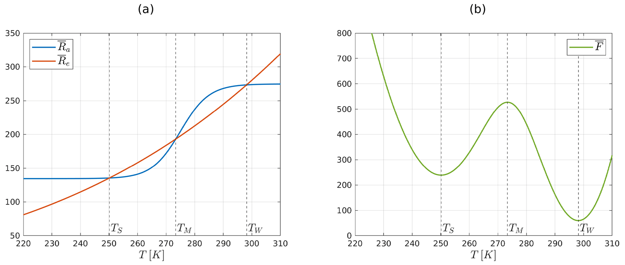
Figure 1(a) Absorbed radiation and emitted radiation for a 0D EBM. The graphs intersect in the three fixed points of the model ; TS and TW are stable, and TM is unstable. (b) Double-well potential associated with the 0D EBM. The function satisfies . The minimum points TS and TW of correspond to stable fixed points.
A one-dimensional (1D) EBM is given by a parabolic partial differential equation where the space variable is one-dimensional (Budyko, 1969; Sellers, 1969; North and Kim, 2017). Denoting the temperature averaged in the zonal direction by , it extends the 0D EBM by introducing the sine of the latitude x=sin (ϕ), where denotes the latitude and t≥0 represents time. We assume that the non-linear radiation balance of the planet, denoted by , depends on the sine of the latitude and on an additive parameter q. This parameter models the effect of carbon dioxide concentration on the radiation budget (Bastiaansen et al., 2022). Atmospheric and ocean transport of heat between latitudes is modelled in a very simplified way by a diffusion term. Assuming spatially homogeneous diffusion in this introductory section and thus ignoring the dependence of κ on latitude and temperature, we obtain a non-degenerate reaction–diffusion equation:
where denotes the Laplace operator in dimension one, the Neumann boundary conditions impose no-heat flux at the poles and is an initial condition. The steady-state solutions of this model, representing the asymptotic solutions for the time-evolving dynamics, correspond to the non-negative solutions u=u(x) of the following elliptic problem:
where u=u(x) depends only on the space variable. This elliptic problem forms a necessary condition for u=u(x) to be our extremal (in particular a local minimizer) for the potential functional
where , and is the square of the norm of u′ in . Calculus of variations is a widely employed technique for studying the existence of a solution to the previous problem (North, 1975; North et al., 1979, 1981; Brezis, 2011). However, proving the existence of a local (but not global) minimum point is generally challenging, and this technique focuses on studying the existence of the global minimum point. The functional Fq in Eq. (6) has another interpretation though which renders it more important than being merely a characterization of solutions to the elliptic problem. Indeed, consider the stochastic partial differential equation (SPDE) on the Hilbert space , given by
obtained by adding a space–time white noise (Wt)t≥0 modelled by a cylindrical Brownian motion on to Eq. (7). R has a cutoff at negative temperature as in Sect. 3.1, and ε>0 is the noise intensity. We refer to Da Prato and Zabczyk (2014) for more details about SPDEs. It can be shown that this SPDE has a unique invariant Gibbs measure ν (Da Prato, 2004), given (broadly speaking) by an expression as in Eq. (3), with Fq replacing (see Sects. 2.1 and 3.1). Therefore, as in the zero-dimensional case, ν concentrates on minimum points of the functional Fq. These minimizers satisfy the elliptic problem (Eq. 5), which therefore describes temperature profiles around which the solutions of the stochastic problem (Eq. 7) tend to cluster.
1.2 Main results and structure of the paper
This paper focuses on the study of the properties and the interpretation of the steady-state solutions of a 1D EBM depending on a bifurcation parameter. Motivated by 0D EBMs, there is a wide consensus in the literature, supported mainly by numerical simulations, regarding the existence of either one or three “interesting” steady-state solutions for 1D EBMs. Firstly, in Theorem 1 we prove the existence of a steady-state solution for the 1D EBM by solving the associated variational problem
i.e. showing the existence of a global minimum point for the functional Fq over a suitable function space 𝕏. Secondly, in Theorem 2 we provide sufficient conditions to have at least three steady-state solutions. These consist of two local minima and one saddle point. The conditions can be summarized as follows:
- i.
the viscosity κ should be sufficiently large,
- ii.
the space-averaged global radiation balance ℛ of the 1D EBM should present a double-well potential with sufficiently deep minimum values attained at the two minimum points.
In essence, the conditions require that steady-state solutions of the spatially inhomogeneous 1D EBM (Eq. 5) are sufficiently well approximated by steady-state solutions of the spatially homogeneous model obtained from spatially averaging the terms in Eq. (5). These assumptions give us the possibility to prove the existence of two minimum points for Fq; further, these minimum points are also close to the minimum points of the space-averaged model. Then, the mountain pass theorem, a classical result from the calculus of variations, enables us to deduce the existence of a third steady-state solution (Ghil and Childress, 1987; Jabri, 2003). Thirdly, we investigate the uniqueness of the solution of the variational problem in terms of the value function
which is the minimum value attained by Fq as a function of q which relates to the greenhouse gas concentration.
- i.
In Theorem 3, we show that V is Lipschitz continuous, thus differentiable except for a Lebesgue zero-measure set;
- ii.
Furthermore, the value function fails to be differentiable if and only if there are two or more co–existing global minimizers for Fq. Moreover, V is concave and hence its derivative V′ is non-increasing.
- iii.
In Corollary 4, we demonstrate how the derivative of V is, up to the sign, the global mean temperature of the global minimum point u0 for Fq. This establishes a one-to-one correspondence between the graph of V and the branch of the bifurcation diagram corresponding to u0.
A byproduct of our analysis is that the global mean temperature is non-increasing with respect to greenhouse gas concentration q. Moreover, it varies continuously with respect to q, as long as there is a unique minimizing temperature profile. However, for greenhouse gas concentration with coexisting global minimizers, the global mean temperature may exhibit as a discontinuous jump as coexisting minimizers cannot all have the same global mean temperature. Furthermore, if a jump occurs, it must necessarily be upward with increasing greenhouse gas concentration.
Our results have a number of interesting physical interpretations. The elliptic 1D EBM not only describes stationary solutions of the time-dependent 1D EBM but moreover characterizes “likely” climates around which the solutions of the stochastic 1D EBM fluctuate. Global minimizers carry special importance as they are exponentially more likely than just local minimizers. Coexistence of global minimizers is just of special interest as these represent equally likely climate scenarios, and intuitively it seems plausible that rapid transitions between those climates are a dominant feature of the dynamics, although this point is not investigated further here. Furthermore coexistence of global minimizers implies a discontinuous change of global mean temperature which will jump upwards with increasing greenhouse gas concentration.
We expect that additional interesting physical conclusions can be drawn through identifying Fq with the (negative) entropy production rate (North and Kim, 2017, Sect. 7.4.2); this will be subject to future work.
This paper is organized as follows. In Sect. 2, we describe the methodology used throughout our work. Firstly, we review the 1D EBM proposed in Bastiaansen et al. (2022). This model serves as the reference for our paper, and it is characterized by the presence of an additive parameter in the radiation budget, which determines the number of steady-state solutions. Secondly, we recall the properties of the steady-state solutions of the 1D EBM that can be obtained from numerical simulations. Finally, we rigorously define the stochastic EBM by introducing space–time white noise. Specifically, we review the invariant measure formula for the resulting reaction–diffusion SPDE. In Sect. 3, we present our novel findings. In Sect. 3.1, we discuss the existence of a solution for the variational problem and outline the properties of the potential functional. Moreover, we explain why the invariant measure of the stochastic EBM concentrates around the global minimum points of the potential functional. Finally, we provide sufficient conditions to demonstrate the existence of at least three steady-state solutions. In Sect. 3.2, we characterize the uniqueness of the solution to the variational problem in terms of the value function. Additionally, we demonstrate that the value function is Lipschitz concave and that its derivative is non-increasing. In Sect. 3.3, we illustrate how knowledge of the value function allows derivation of a portion of the bifurcation diagram and vice versa. In Sect. 4, we offer a comprehensive summary of our work. In Appendix A, we describe the finite difference method employed to conduct the numerical simulations presented in this study. Furthermore, the Supplement includes rigorous proofs of our main results.
2.1 A 1D energy balance model
The fundamental mechanism of 1D EBMs is that the temperature , averaged in the zonal direction, evolves in time due to (i) the diffusion of energy between adjacent regions, (ii) the energy absorbed by the planet and (iii) the energy emitted by the planet. The 1D EBM we consider in this paper is a Seller-type EBM where the absorbed radiation depends on an additive parameter (Bastiaansen et al., 2022). We only add a change in the diffusion term in order to get a non-degenerate parabolic PDE. Given an initial condition , the non-linear, parabolic, reaction–diffusion PDE governing the model is given by
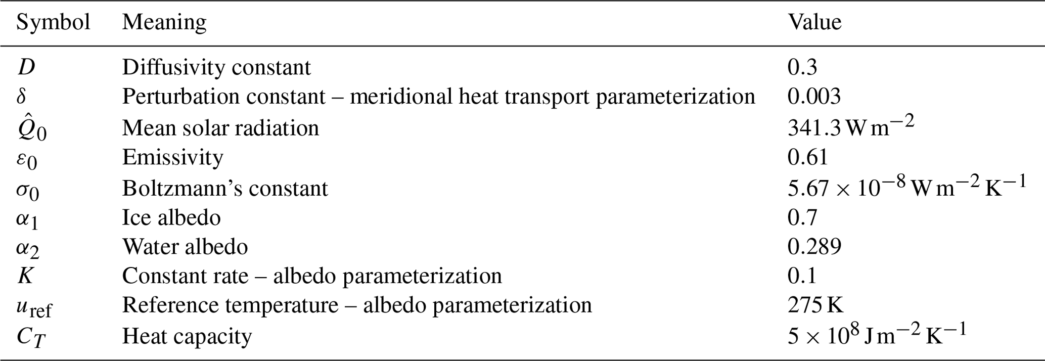
where Ra and Re represent the radiation absorbed and emitted by the planet per unit area, respectively. CT is the heat capacity, and the differential term parameterizes the meridional heat transport. The boundary conditions impose no flux at the poles. We now provide further details regarding the parameterization of these terms. The values of the constants of the model can be found in Table 1.
Firstly, the absorbed radiation is assumed to have the following form:
where Q0 is the solar radiation per unit area, and α is the albedo. The solar radiation is assumed to be
where is the mean solar radiation, and ci represents constants. The albedo, which is the proportion of the incident light or radiation that is reflected by a surface, is parameterized by a smooth monotonically decreasing function with a peak derivative in a reference temperature uref close to the melting point of ice. Specifically,
where K>0 is a rate parameter and α1>α2 are respectively the ice albedo and the water albedo.
Second, the emitted radiation is modelled using the Stefan–Boltzmann law, in other words assuming that the Earth radiates as a black body. Under this assumption, the energy radiated is proportional to the fourth power of its temperature and it is given by
where ε0 and σ0 are respectively the emissivity and Boltzmann's constant. The additive parameter q describes, in a simplified way, the radiative forcing by CO2, i.e. the effect of atmospheric CO2 on the energy budget (IPCC, 2014). It is worth explaining (i) the additive structure of q and (ii) its independence on the spatial variable x. About the first point, denote by C the global CO2 concentration in part per million (ppm) and assume, just for explanation purposes, a dependence of the outgoing radiation both on u and C. To avoid confusion, we denote this by , the outgoing radiation depending on temperature and CO2 concentration. If we linearize with respect to temperature, we get
where is a reference temperature. In Myhre et al. (1998), three radiative transfer models are used in order to get that the dependence of the outgoing radiation with respect to changes in CO2 is given by
where C0 is a reference CO2 concentration, and are explicit constants. In conclusion,
and thus the radiative forcing of CO2 has an additive structure. About point (ii), we adopt the well-mixed hypothesis for CO2. In other words, we assume that atmospheric CO2 is globally homogeneous, thereby inducing a radiative forcing q independent of latitude (IPCC, 2001). This assumption overlooks the spatial pattern of CO2 concentration, which affects many aspects of the climate system, such as the poleward heat transport (Huang et al., 2017). It was the state-of-the-art assumption 2 decades ago, although today it is common to keep in consideration the spatial distribution of radiative forcing (IPCC, 2001; Byrne and Goldblatt, 2014; Zhang et al., 2019).
The third component of the model is the term ∂x(κ(x)ux). It parameterizes the meridional heat transport, that is, the phenomenon resulting from the poleward transportation of heat by the Earth–atmosphere system due to the surplus of net radiation heating in the tropics and the deficit in the poleward regions. Usually, the diffusion function κ(x) is assumed null at the poles, i.e. with a form such as , where D is a diffusion constant. This choice is based on the paradigm of mimicking the conduction of heat on a sphere; see North and Kim (2017) for a derivation. On the other hand, it leads to mathematical difficulties in the treatment of the singular PDE arising, in particular in the study of the corresponding variational problem, from which all our results follow. To avoid these difficulties, which at the moment remain an open problem to solve, we add as a simplifying assumption that κ is non-degenerate and given by
We choose δ=0.003, but its value is not important for the results of this work, and different choices can be made.
For the parabolic problem (Eq. 8), the global existence and uniqueness of the solution can be demonstrated, given a regular initial condition (Temam, 1997). Furthermore, if the initial condition is non-negative, the solution remains non-negative for any time t>0. This can be shown proving that is an invariant region for Eq. (8), exploiting the fact that there exist such that for all and (Smoller, 2012).
We recall the formulation of stochastic EBMs using the theory of SPDEs (Da Prato and Zabczyk, 2014). Denote by Δ the Laplace operator with Neumann boundary conditions. Given an initial condition , we consider the following SPDE:
where ε>0, and (Wt)t≥0 is a cylindrical Brownian motion on H. Under the minor cutoff modifications introduced in Sect. 3.1, it can be proved that the H-valued stochastic process (ut)t which solves in a mild sense (9) is unique and has continuous trajectories (Da Prato and Zabczyk, 2014). In addition to this there exists a unique Gibbs invariant measure
where ℛ is as in Eq. (6), and is a symmetric Gaussian measure on H with covariance (Da Prato, 2004, 2006). The covariance operator is the unique linear operator such that for each , where denotes the scalar product in H. Further, it can be shown that 𝒬 is symmetric and positive-definite, and its eigenvalues (λk)k∈ℤ satisfy . In the following lines, given a symmetric, positive-definite operator 𝒬 such that , we are going to explain how to construct an H-valued random variable X with law 𝒩(0,𝒬). Indeed, consider a sequence (Rk)k∈ℤ of independent and identically distributed ℝ-𝒩(0,1) random variables defined on a probability space . We can assume without loss of generality that the eigenvectors (ek)k∈ℤ associated with the eigenvalues (λk)k∈ℤ form an orthonormal basis of H. Then, the H-valued random variable
is well defined, i.e. the series defining X converges in and has law 𝒩(0,𝒬) (Da Prato, 2006, Proposition 2.18). Further, the convergence also holds ℙ almost surely in H (Da Prato, 2006, Proposition 2.13).
As mentioned in the introduction, this measure is concentrated on minimum points of the functional Fq. A heuristic explanation of this fact can be found in Sect. 3.1.
The stationary problem associated with the 1D EBM is given by the elliptic equation for u=u(x):
These solutions can be either stable or unstable, depending on the long-term behaviour of their infinitesimal perturbations. As pointed out in Bastiaansen et al. (2022), if the reaction–diffusion equation for was space-homogeneous, i.e. of the form
then the stable steady-state solutions would correspond to functions that are constant in space and time, with values given as the roots of
A rigorous result in this direction has been shown in Gaspar and Guaraco (2018). Indeed, for a fixed double-well symmetric potential, it has been proved that (i) if κ is large enough, the only steady-state solutions of Eq. (12) are the constants where the potential is critical, and (ii) the number of unstable steady-state solutions to Eq. (12) can be made arbitrarily large as κ→0. Introducing a spatial dependence in leads to a space-heterogeneous model. Depending on the space heterogeneity, it can exhibit any number of both stable and unstable steady-state solutions (Bastiaansen et al., 2022). The variational approach to the study of steady-state solutions provides a tool for characterizing the stable ones, which are the local minimum points of a functional.
In the following paragraph, we describe the properties of the solutions of Eq. (11). As the parameter q changes, numerical simulations for Eq. (11) suggest the existence of either one or three steady-state solutions. That is, there exists q1<q2 s.t. Eq. (8) has one steady-state solution if q<q1 or q>q2, and the steady-state solutions are three if . In the latter case, we denote the solutions by , corresponding respectively to the snowball climate, a middle (or intermediate) climate and the warm climate. As an analogy, we denote by uS the unique steady-state solution for q<q1 and by uW the unique one for q>q2. Figure 2a shows the bifurcation diagram of the model in the plane, where denotes the average temperature. Figure 2b depicts the three steady-state solutions for .
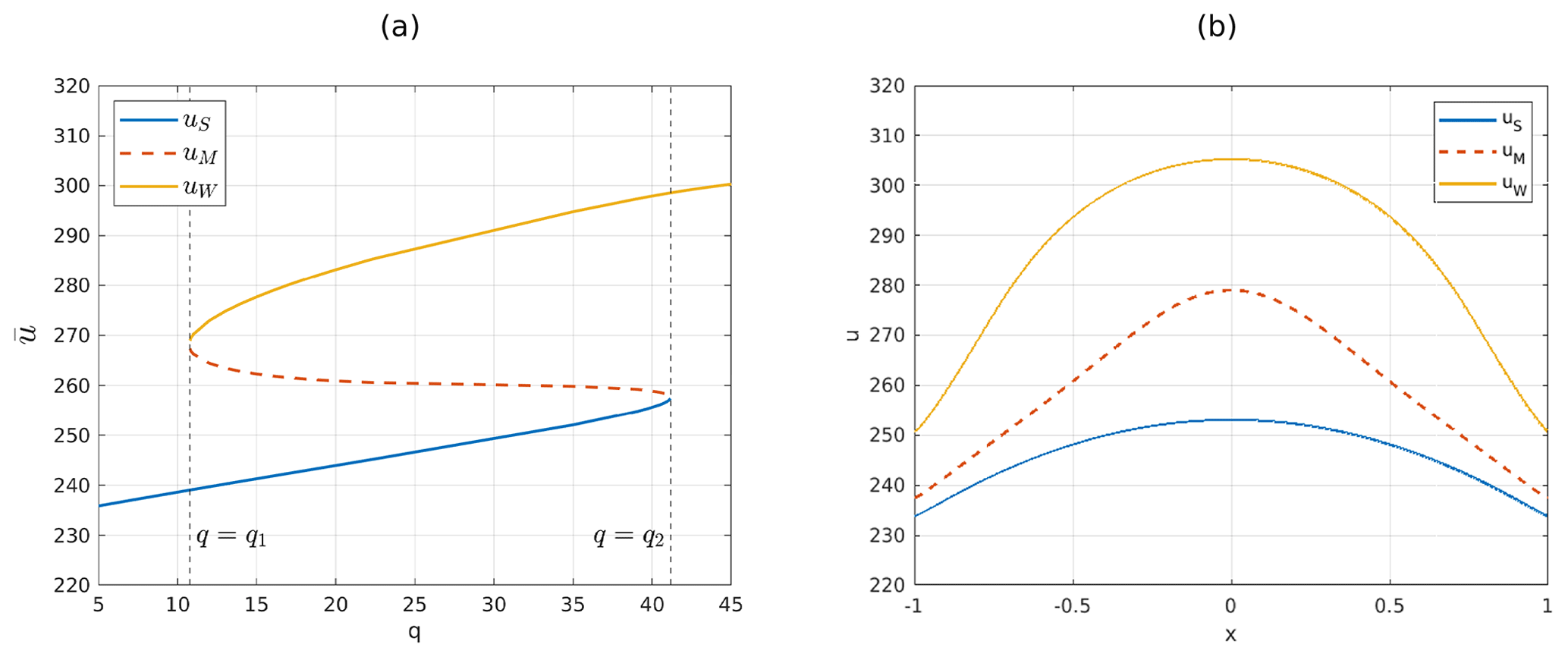
Figure 2(a) Bifurcation diagram of the steady-state solutions in the plane, with . Solid lines denote stable solutions uS and uW, while dashed lines denote the unstable solution uM. (b) Steady-state solutions of the EBM for q=25. In every point x of the space domain, the three steady-state solutions satisfy , with maximum temperature attained at the Equator and minimum temperature attained at the poles.
A stability analysis can be conducted to determine the stability of the steady-state solutions. The results show that uS and uW are stable, while the middle climate, uM, is unstable. Furthermore, it is worth noting that special values correspond to bifurcation points of saddle-node type, where the unstable solution uM collides with either uW (for q=q1) or uS (for q=q2) and then disappears. These numerical findings regarding the number and stability of the steady-state solutions will be supported and validated using rigorous arguments, as in the next section.
Table 1Parameters and constants appearing in the Seller EBM (8).
3.1 Potential functional and its minimizer
In this section, we (i) provide an intuitive motivation for why the invariant measure for the stochastic EBM concentrates on minimum points of the functional Fq, (ii) prove the existence of global minimum points for Fq using the direct method, and (iii) present sufficient conditions on the viscosity κ and the space-averaged potential , with , to ensure that the 1D EBM has at least three steady-state solutions.
Firstly, consider the stochastic EBM (9). Assume that for a negative value of u, where the model has no physical meaning, the Stefan–Boltzmann law is extended as
And β is smoothly extended to by setting it to zero outside the physically relevant range, as described in the Supplement. Then, Eq. (9) possesses a unique Gibbs invariant probability measure given by
where is the positive part, denotes a symmetric Gaussian measure with covariance operator over the Hilbert space and Z is the normalization constant. See Da Prato (2004) for a rigorous derivation of the invariant measure for a reaction–diffusion model with a polynomial homogeneous reaction term. We move to explain in what sense ν is concentrated around minimum points of Fq. In fact, for u∈H the Gaussian measure μ is formally given by
where Here, Z1 is a normalization constant, denotes the scalar product in H and du is a formal notation for the Lebesgue measure on H. If we perform an integration by parts, we get
Plugging the previous identity into Eq. (10), we obtain
From this heuristic formula, we see that points u such that Fq(u) is not a global minimum have exponentially smaller density than the minimum points. Indeed, if u1 is a global minimum point and u≠u1, then the mass given by ν in a small neighbourhood around u is exponentially smaller than the mass given to a neighbourhood of the same size around u1; in particular, the ratio between the two masses is given by . The previous derivation is formal, because the Lebesgue measure cannot be defined on an infinite-dimensional Hilbert space. For a more rigorous explanation, see Sect. S2 in the Supplement.
Next, we discuss the properties of the functional given by
where B is a primitive of the co-albedo , and denotes the Sobolev space of order 1 and exponent 2, i.e. the function space where a function u and its derivative u′ (in a weak sense) are both square integrable over . See Brezis (2011) for more details about Sobolev spaces. The functional Fq, depending on the parameter q, is known in the literature as a potential functional or Lyapunov function (North et al., 1979; North and Kim, 2017). The study of the functional Fq gives useful information thanks to its links with the invariant measure for the stochastic 1D EBM, as we have seen, and the stable steady-state solutions for the deterministic 1D EBM which emerge as necessary conditions for the stationarity of Fq. Going deeper with the former point, the first variation of Fq in the point u in direction h is given by
where in the last identity we have used integration by parts. Since h is arbitrary, u is a stationary point for the functional Fq if and only if it is a steady-state solution for the EBM. In particular, local extremum points for Fq correspond to steady-state solutions of the EBM. Any local minimizer of Fq represents a locally attractive solution of the deterministic 1D EBM. In view of our interpretation of Fq in terms of the invariant measure, however, global minimizers play a special role since if present and unique they are exponentially more likely than any other state (including minimizers that are just local). The following result establishes the existence of a global minimum point for Fq.
If q>0, then there exists a global regular non-negative minimizer for Fq. In other words, if we consider the variational problem
then there exists u0∈C∞ such that u0 is a solution of the EBM and
In addition to this, if q belongs to a bounded interval, then u can be bounded uniformly with respect to q:
A rigorous proof of the previous result can be found in Sect. S3. The proof relies on standard arguments from the direct method of calculus of variation, exploiting the fact that the outgoing radiation in the EBM model prevents the temperature from being too high.
Concerning the existence of two local minimum points, let us describe a sufficient condition. Consider the potential function coming from the space-averaged model
If the viscosity κ>0 is sufficiently large and the function has a double-well shape with sufficiently deep minimum values attained at the minimum points, then we are able to prove the existence of two minimum points for Fq. Further, it is possible to prove that the functional Fq satisfies a compactness condition known as the Palais–Smale condition. This property and the mountain pass theorem give the possibility to deduce the existence of a third steady-state solution. Next, we characterize a situation in which there are three steady-state solutions, two of which are local minimizers (Jabri, 2003). This is summarized in the following result.
Denote by the open ball in H1 with centre v and radius ρ>0. Assume has two non-negative minimum points u1≠u2, with Fq(u1)≥Fq(u2). Then, there exist ω>0 and as such that if satisfies
- i.
, for ;
- ii.
;
- iii.
;
then has two local minimum points, , such that
- a.
;
- b.
for .
- c.
If , then , with
Note how the previous result can be also interpreted as giving sufficient conditions for the convergence of the stable solutions of a space-inhomogeneous EBM to the stable solution of the corresponding space-averaged model, as the diffusion becomes large.
3.2 Value function and uniqueness for the functional minimizer
The key element of this section is the value function, which is given by
From Sect. 3.1, we know that the previous infimum is indeed a minimum, and so V(q) can be interpreted as the minimum possible value attained by the potential functional over the possible temperature profiles u. Since a minimum point for Fq is also a stationary point for the functional, the value function can be evaluated numerically by computing the minimum of the three steady-state solutions uS,uM and uW. Following this strategy, Fig. 3 shows , with . Particularly, there exists a point q3 such that uS is the global minimum point of Fq for q<q3, while uW is the global minimum point for q>q3. Further, for q=q3 the function Fq has two different global minimum points uS and uW, and q=q3 corresponds a non-differentiability point for V. In addition to this, the value function appears to be concave, thus with a decreasing derivative, where it exists.
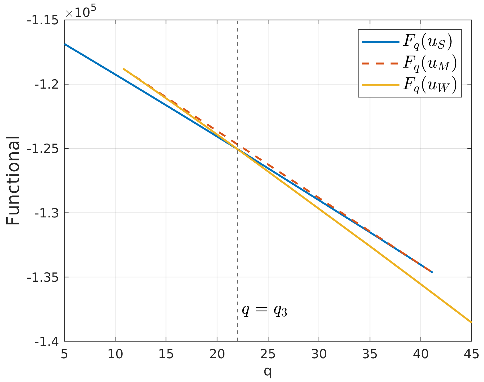
Figure 3Potential functional Fq evaluated in the three steady-state solutions uS,uM and uW. For q<q3, uS is the global minimum point, while uW is a local minimum point. On the other hand, for q>q3 the opposite happens. Solid lines correspond to values of the functional attained on stable solutions; dashed lines are for values corresponding to unstable ones.
Summarizing, the numerical evaluations of V(q) suggest the following result, a rigorous proof of which is included in the Supplement.
Assume q belongs to a bounded interval. Then
- i.
V is Lipschitz continuous.
- ii.
q is a non-differentiable point for V if and only if there is more than one minimizer for Fq.
- iii.
V is concave and V′ is non-increasing.
We also see numerically that uM is actually never a global minimizer for the specific functional Fq considered here, but we do no have rigorous proof of this fact. Let us briefly discuss the proofs of the previous points. The proof of (i) follows from the facts that the sup norm of the minimizer u0 can be bounded uniformly in q and that, given a family {gi}i∈I of Li Lipschitz functions gi, the is Lipschitz continuous if the constants Li can be bounded uniformly. In our case, given u∈H1 is non-negative, we have
where M>0 is the constant appearing in Eq. (15). On the other hand, the proof of point (ii) is less straightforward, although being very similar to the one for the existence of a solution for the variational problem. The proof of point (iii) makes use of the concept of semiconcavity, a generalization of that of concavity, which is fundamental in optimal control (Cannarsa and Sinestrari, 2004). The main reason for the concavity of V though is that V is an infimum over functions that are affine in q. Hence, the fact that q is additive is essential for this result. More details can be found in Sects. S4 and S5 in the Supplement.
3.3 Value function graph and bifurcation diagram
An additional property of the value function can be observed when comparing the bifurcation diagram (Fig. 4a) and the graph of the value function (Fig. 3).
Corollary 4. If V is differentiable, then
, where u0 is the only minimizer for Fq.
In other words, the part of the bifurcation diagram that corresponds to the global minimizer, represented by the subgraph , can be determined based on the knowledge of V′, and vice versa. Figure 4 compares Figs. 2a and 3, highlighting in magenta the corresponding parts of the two graphs. From the mathematical point of view, the previous result is a consequence of the proof of Theorem 3.
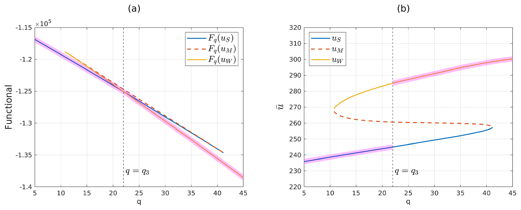
Figure 4Comparison between the value function graph (left) and bifurcation diagram (right) for the 1D EBM. The magenta-shaded area highlights the parts of the plots which are in one-to-one correspondence. (a) Functional Fq evaluated on steady-state solutions, as in Fig. 3. (b) Bifurcation diagram, as in Fig. 2a.
It is worth pointing out that by combining Theorem 3 and Corollary 4, a valuable property emerges, i.e. the global mean temperature of the functional minimizer is non-decreasing with respect to q. In other words, as the concentration of CO2 rises, the global mean temperature increases. Additionally, through this monotonicity and Froda's theorem (Rudin, 1976, Theorem 4.30), we also establish that the global mean temperature is continuous, except for, at most, a countable number of upward jumps.
In the second part of this section, we demonstrate the applicability of Corollary 4 to other reaction–diffusion equations. We use as an example a spatially heterogeneous Allen–Cahn equation (ACE), already considered in Bastiaansen et al. (2022). For an initial condition , this model is given by
The associated elliptic problem for u=u(x) is
In this case, the potential functional takes the form
and all the properties discussed in Sect. 3.1 and 3.2 can be extended to this equation. Specifically, Theorems 1, 2 and 3 hold. But in this case, the structure of the bifurcation diagram is more complex, even if symmetric with respect to q=0. Indeed, through numerical experiments, it is possible to deduce the existence of such that (a) for |q|>q5 or |q|<q4, there exists a single steady-state solution, which is stable, (b) for there are three steady-state solutions, two of which are stable while the third is unstable. Further, are bifurcation points of the saddle-node type. We denote by u1 the steady-state solution for , by u2 and u3 the steady-state solutions appearing at the bifurcation point and existing for in addition to u1, and by u4 and u5 the steady-state solutions appearing at q=q4 and existing for in addition to u3. Regarding the potential functional Jq, in this case there exists such that u1 is the global minimum point for the functional for , and u3 is the global minimum point for , while u5 becomes the global minimum point for q>q6. A picture for the bifurcation diagram just described and the value function is shown in Fig. 5. Note that represents the only values of the parameter q for which the value function is not differentiable and also the only points in which the global minimizer of the variational problem is not unique.
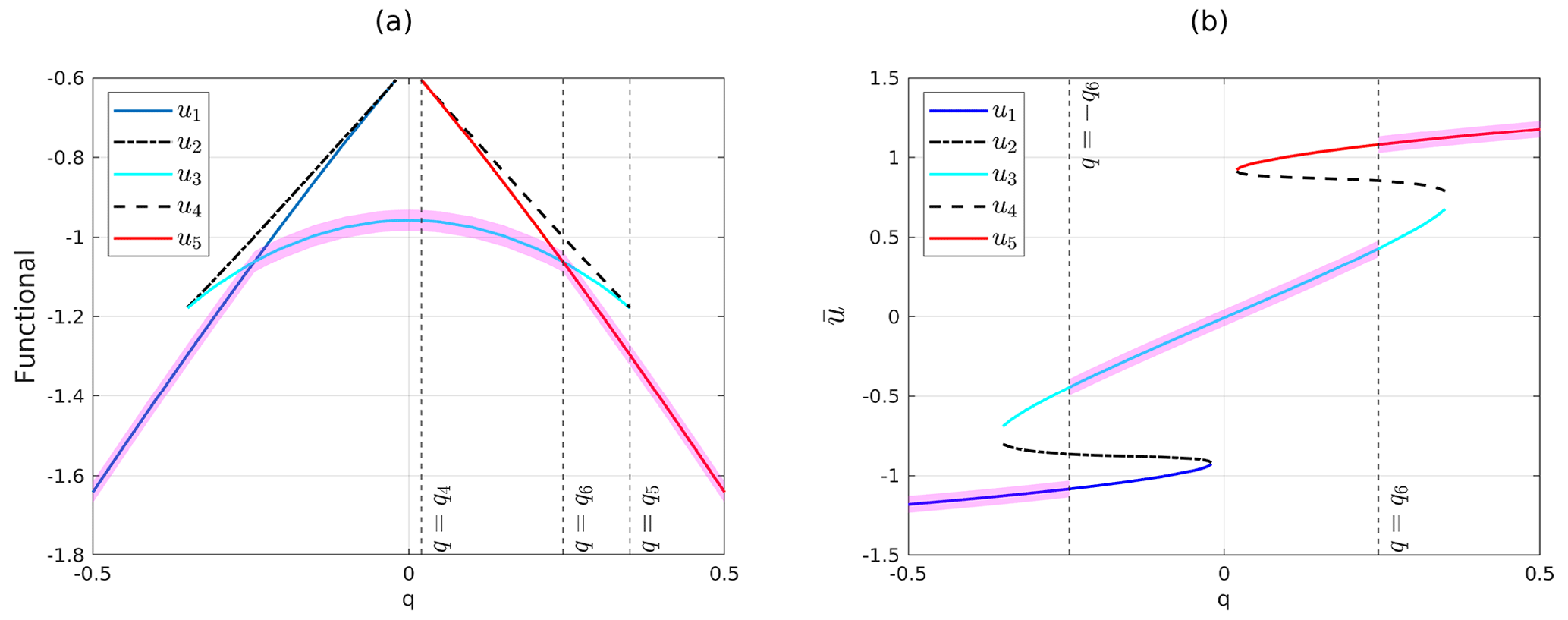
Figure 5Comparison between the value function and the bifurcation diagram for the non-homogeneous ACE. The magenta-shaded area highlights the parts of the plots which are in one-to-one correspondence. (a) Potential functional evaluated on the steady-state solutions: u1 is the global minimum point for , u3 is the global minimum point for , u5 is the global minimum point for q>q6. Note that are the non-differentiability point for the value function, corresponding to non-uniqueness of the minimizer. (b) Bifurcation diagram.
In this paper, we have considered a one-dimensional energy balance model depending on a bifurcation parameter q, describing the effect of CO2 concentration in the atmosphere and affecting the energy absorbed by the planet. Numerical simulations show that this model can exhibit either one or three asymptotic solutions, depending on the values of q. We began our analysis by introducing the potential functional Fq associated with the steady-state solutions. The functional Fq has significant implications, as it is closely linked to both the stability of steady-state solutions of the EBM and the invariant measure for the stochastic EBM obtained by perturbing the model with an additive Gaussian white noise. In particular, the invariant measure of the system concentrates on global minimizers of Fq, giving them exponentially larger weight than local minimizers. By analysing the first variation of Fq and applying standard arguments from the direct method of calculus of variations, we established that Fq possesses a global regular minimizer for all values of the parameter q. Furthermore, we provide sufficient conditions to prove the existence of at least three steady-state solutions for the 1D EBM.
We then introduced the value function V(q), which represents the minimum value attained by the potential functional among all possible temperature profiles. By evaluating V(q) numerically using the steady-state solutions uS,uM and uW, we observed that the function exhibits Lipschitz continuity and concavity. Furthermore, non-differentiability points of V(q) coincide with points where multiple global minimizers exist for Fq. Lastly, when V is differentiable, its derivative is non-increasing and equal to the negative global mean temperature, i.e. , where u0 is the minimizer for Fq. Moreover, as a consequence of the explicit expression for V′, the global mean temperature is non-decreasing with respect to q, and it is continuous, except for a Lebesgue zero-measure set of upwards jumps. These are the non-differentiability points of V, corresponding to the case where two or more global minimizers, hence multiple climates equally probable, exist for the stochastic EBM. These findings, which we are able to prove rigorously, allow us to establish a correspondence between the bifurcation diagram and the graph of the value function. Additionally, we applied our results to a spatially inhomogeneous Allen–Cahn equation to show how our results still hold for more general space-inhomogeneous reaction–diffusion equations.
The diffusion function κ=κ(x) that we have examined is non-degenerate at the boundary of the spatial domain. As noted in Sect. 2.1, this is an assumption to simplify the study of the variation problem. At present, there remains a problem with how to extend our results to the case where κ is degenerate at the boundary.
Regarding the impact of our work on current climate change, we have characterized climate as an invariant measure within a stochastic equation that describes temperature. The emission of CO2 is considered a parameter influencing the shape of this invariant measure, particularly in relation to the points around which the measure is concentrated. From our perspective, the climate we are currently witnessing reflects changes in the invariant measure, representing a realization of a random variable with that invariant measure as its distribution. Moreover, we have demonstrated the monotonic relationship between global mean temperature and CO2. Finally, we have outlined simple conditions, adaptable to other multi-stable reaction–diffusion models, to establish the existence of three asymptotic climate states.
Concerning future development of this work, one interesting aspect we are working on is to understand how the invariant measure for the stochastic EBM changes close to bifurcation points. This points in the direction of using statistical indicators to detect the approach of tipping points, which in our model correspond to points of discontinuity of the global mean temperature with respect to the parameter q.
In this section, we describe the numerical method adopted to approximate the solutions of the elliptic problem (11) numerically. We used a classical finite difference scheme, which we are going to illustrate (Quarteroni and Valli, 2008; Thomas, 2013). To simplify the notation, let's define
as the non-linear reaction term. We consider a uniform mesh for made of n+1 points
Then, the solution to the problem can be approximated by considering the following system:
where u−1and un+1 are ghost points, and
The system of equations can be written in vector form as
with and . At this point, multiplying the first equation by , subtracting the second one and dividing by 2, we get
In a symmetric way, multiplying the last equation by , subtracting the second last equation and dividing by 2, we get
In this way, the Neumann version of the elliptic problem has the following form:
and consists of a set of (n+3) non-linear equations, whose solution u can be approximated using the Newton–Raphson method (NRM). The initial guess used to start the iteration in NRM is obtained via a shooting method, thus reducing the boundary value problem given by the elliptic PDE in Eq. (11) to an initial value problem (IVP). A linear search is applied to find the shooting parameter, i.e. the initial condition of the IVP. Lastly, the solution of the IVP is approximated using the classical Euler's method for ODEs.
This work does not include any externally supplied code, data, or other material. All material in the text and figures was produced by the authors using standard mathematical and numerical analysis by the authors. The code is available at Zenodo (https://doi.org/10.5281/zenodo.10469451, Del Sarto et al., 2024).
The supplement related to this article is available online at: https://doi.org/10.5194/npg-31-137-2024-supplement.
GDS conceptualized the paper, performed the numerical simulations, and took the lead role in writing and revising the paper. JB, FF and TK conceptualized the paper and supervised the writing. All authors provided critical feedback and helped shape the research.
The contact author has declared that none of the authors has any competing interests.
Views and opinions expressed are those of the authors only and do not necessarily reflect those of the European Union or the European Research Council. Neither the European Union nor the granting authority can be held responsible for them.
Publisher’s note: Copernicus Publications remains neutral with regard to jurisdictional claims made in the text, published maps, institutional affiliations, or any other geographical representation in this paper. While Copernicus Publications makes every effort to include appropriate place names, the final responsibility lies with the authors.
We are very grateful to the referee for carefully reading the paper and for their valuable comments. We acknowledge fruitful discussions with Valerio Lucarini and Robbin Bastiaansen. Gianmarco Del Sarto would like to thank the Department of Mathematics and Statistics, University of Reading, for its hospitality. Tobias Kuna and Jochen Bröcker would like to thank the Scuola Normale Superiore for its hospitality. Gianmarco Del Sarto is supported by the Italian national interuniversity PhD course in sustainable development and climate change.
Franco Flandoli's research is funded by the European Union (ERC, NoisyFluid, no. 101053472).
This paper was edited by Natale Alberto Carrassi and reviewed by two anonymous referees.
Ashwin, P., Wieczorek, S., Vitolo, R., and Cox, P.: Tipping points in open systems: bifurcation, noise-induced and rate-dependent examples in the climate system, Philos. T. Roy. Soc. A, 370, 1166–1184, https://doi.org/10.1098/rsta.2011.0306, 2012. a
Baldi, P.: Stochastic Calculus, Springer International Publishing, https://doi.org/10.1007/978-3-319-62226-2, 2017. a
Bastiaansen, R., Dijkstra, H. A., and von der Heydt, A. S.: Fragmented tipping in a spatially heterogeneous world, Environ. Res. Lett., 17, 045006, https://doi.org/10.1088/1748-9326/ac59a8, 2022. a, b, c, d, e, f, g
Berger, A. (Ed.): Climatic Variations and Variability: Facts and Theories, Springer, Netherlands, https://doi.org/10.1007/978-94-009-8514-8, 1981. a
Brezis, H.: Functional analysis, Sobolev spaces and partial differential equations, vol. 2, Springer, https://doi.org/10.1007/978-0-387-70914-7, 2011.Please provide persistent identifier (DOI preferred). a, b
Budyko, M. I.: The effect of solar radiation variations on the climate of the Earth, Tellus, 21, 611–619, 1969. a, b
Byrne, B. and Goldblatt, C.: Radiative forcing at high concentrations of well‐mixed greenhouse gases, Geophys. Res. Lett., 41, 152–160, https://doi.org/10.1002/2013gl058456, 2014. a
Cannarsa, P. and Sinestrari, C.: Semiconcave Functions, Hamilton–Jacobi Equations, and Optimal Control, Birkhäuser Boston, ISBN 9780817644130, https://doi.org/10.1007/b138356, 2004. a
Cannarsa, P., Lucarini, V., Martinez, P., Urbani, C., and Vancostenoble, J.: Analysis of a two-layer energy balance model: long time behaviour and greenhouse effect, arXiv [preprint], https://doi.org/10.48550/arXiv.2211.15430, 2022. a
Da Prato, G.: Kolmogorov Equations for Stochastic PDEs, Birkhäuser, Basel, https://doi.org/10.1007/978-3-0348-7909-5, 2004. a, b, c
Da Prato, G.: An Introduction to Infinite-Dimensional Analysis, Springer, Berlin, Heidelberg, https://doi.org/10.1007/3-540-29021-4, 2006. a, b, c
Da Prato, G. and Zabczyk, J.: Stochastic Equations in Infinite Dimensions, Cambridge University Press, https://doi.org/10.1017/cbo9781107295513, 2014. a, b, c
Del Sarto, G., Flandoli, F., Kuna, T., and Bröcker, J.: Variational Techniques for a One-Dimensional Energy Balance Model (Version MatlabR2023b), Zenodo [code], https://doi.org/10.5281/zenodo.10469451, 2024. a
Díaz, J. I.: On the mathematical treatment of energy balance climate models, in: The Mathematics of Models for Climatology and Environment, edited by: Díaz, J. I., Springer, Berlin Heidelberg, Berlin, Heidelberg, 217–251, ISBN 978-3-642-60603-8, 1997. a
Díaz, J., Langa, J., and Valero, J.: On the asymptotic behaviour of solutions of a stochastic energy balance climate model, Phys. D, 238, 880–887, https://doi.org/10.1016/j.physd.2009.02.010, 2009. a
Gaspar, P. and Guaraco, M. A.: The Allen–Cahn equation on closed manifolds, Calc. Var. Partial Dif., 57, 1–42, 2018. a
Ghil, M.: Climate Stability for a Sellers-Type Model, J. Atmos. Sci., 33, 3–20, https://doi.org/10.1175/1520-0469(1976)033<0003:CSFAST>2.0.CO;2, 1976. a
Ghil, M. and Childress, S.: Topics in Geophysical Fluid Dynamics: Atmospheric Dynamics, Dynamo Theory, and Climate Dynamics, Springer, New York, https://doi.org/10.1007/978-1-4612-1052-8, 1987. a
Ghil, M. and Lucarini, V.: The physics of climate variability and climate change, Rev. Mod. Phys., 92, 035002, https://doi.org/10.1103/RevModPhys.92.035002, 2020. a, b
Hasselmann, K.: Stochastic climate models Part I. Theory, Tellus, 28, 473–485, https://doi.org/10.1111/j.2153-3490.1976.tb00696.x, 1976. a
Huang, Y., Xia, Y., and Tan, X.: On the pattern of CO2 radiative forcing and poleward energy transport, J. Geophys. Res., 122, 10578–10593, 2017. a
Imkeller, P.: Energy balance models – viewed from stochastic dynamics, in: Stochastic Climate Models, edited by: Imkeller, P. and von Storch, J.-S., Birkhäuser Basel, Basel, 213–240, ISBN 978-3-0348-8287-3, 2001. a, b
IPCC: Climate Change 2001: The Scientific Basis, Contribution of Working Group I to the Third Assessment Report of the Intergovernmental Panel on Climate Change, edited by: Houghton, J. T., Ding, Y., Griggs, D. J., Noguer, M., van der Linden, P. J., Dai, X., Maskell, K., and Johnson, C. A., Cambridge University Press, Cambridge, United Kingdom and New York, NY, USA, 881 pp., ISBN 9780521014953, 2001. a, b
Intergovernmental Panel on Climate Change (IPCC): Climate Change 2013 – The Physical Science Basis: Working Group I25 Contribution to the Fifth Assessment Report of the Intergovernmental Panel on Climate Change, Cambridge University Press, https://doi.org/10.1017/CBO9781107415324, 2014. a
Jabri, Y.: The Mountain Pass Theorem, Cambridge University Press, https://doi.org/10.1017/cbo9780511546655, 2003. a, b
Lelièvre, T. and Stoltz, G.: Partial differential equations and stochastic methods in molecular dynamics, Acta Numer., 25, 681–880, https://doi.org/10.1017/s0962492916000039, 2016. a
Lenton, T. M., Held, H., Kriegler, E., Hall, J. W., Lucht, W., Rahmstorf, S., and Schellnhuber, H. J.: Tipping elements in the Earth's climate system, P. Natl. Acad. Sci. USA, 105, 1786–1793, 2008. a
Lenton, T. M., Livina, V. N., , V., van Nes, E. H., and Scheffer, M.: Early warning of climate tipping points from critical slowing down: comparing methods to improve robustness, Philos. T. Roy. Soc. A, 370, 1185–1204, https://doi.org/10.1098/rsta.2011.0304, 2012. a
Lucarini, V. and Bódai, T.: Transitions across melancholia states in a climate model: Reconciling the deterministic and stochastic points of view, Phys. Rev. Lett., 122, 158701, https://doi.org/10.1103/PhysRevLett.122.158701, 2019. a
Lucarini, V., Serdukova, L., and Margazoglou, G.: Lévy noise versus Gaussian-noise-induced transitions in the Ghil–Sellers energy balance model, Nonlin. Processes Geophys., 29, 183–205, https://doi.org/10.5194/npg-29-183-2022, 2022. a
Myhre, G., Highwood, E. J., Shine, K. P., and Stordal, F.: New estimates of radiative forcing due to well mixed greenhouse gases, Geophys. Res. Lett., 25, 2715–2718, https://doi.org/10.1029/98gl01908, 1998. a
North, G. R.: Theory of Energy-Balance Climate Models, J. Atmos. Sci., 32, 2033–2043, https://doi.org/10.1175/1520-0469(1975)032<2033:TOEBCM>2.0.CO;2, 1975. a, b
North, G. R.: Multiple solutions in energy balance climate models, Global Planet. Change, 2, 225–235, https://doi.org/10.1016/0921-8181(90)90003-U, 1990. a
North, G. R. and Cahalan, R. F.: Predictability in a Solvable Stochastic Climate Model., J. Atmos. Sci., 38, 504–513, https://doi.org/10.1175/1520-0469(1981)038<0504:PIASSC>2.0.CO;2, 1981. a
North, G. R. and Kim, K.-Y.: Energy Balance Climate Models, Wiley, https://doi.org/10.1002/9783527698844, 2017. a, b, c, d, e
North, G. R., Howard, L., Pollard, D., and Wielicki, B.: Variational Formulation of Budyko-Sellers Climate Models, J. Atmos. Sci., 36, 255–259, https://doi.org/10.1175/1520-0469(1979)036<0255:VFOBSC>2.0.CO;2, 1979. a, b
North, G. R., Cahalan, R. F., and Coakley, J. A.: Energy balance climate models, Rev. Geophys., 19, 91–121, https://doi.org/10.1029/rg019i001p00091, 1981. a
Quarteroni, A. and Valli, A.: Numerical approximation of partial differential equations, vol. 23, Springer Science & Business Media, https://doi.org/10.1007/978-3-540-85268-1, 2008. a
Rudin, W.: Principles of Mathematical Analysis, 3rd Edn., ISBN 9780070542358, 1976. a
Scheffer, M., Bascompte, J., Brock, W., Brovkin, V., Carpenter, S., Dakos, V., Held, H., Nes, E., Rietkerk, M., and Sugihara, G.: Early-Warning Signals for Critical Transitions, Nature, 461, 53–9, https://doi.org/10.1038/nature08227, 2009. a
Sellers, W. D.: A Global Climatic Model Based on the Energy Balance of the Earth-Atmosphere System, J. Appl. Meteorol. Clim., 8, 392–400, https://doi.org/10.1175/1520-0450(1969)008<0392:AGCMBO>2.0.CO;2, 1969. a, b
Smoller, J.: Shock waves and reaction–diffusion equations, vol. 258, Springer Science & Business Media, https://doi.org/10.1007/978-1-4612-0873-0, 2012. a
Temam, R.: Infinite-Dimensional Dynamical Systems in Mechanics and Physics, Springer, New York, https://doi.org/10.1007/978-1-4612-0645-3, 1997. a
Thomas, J. W.: Numerical partial differential equations: finite difference methods, vol. 22, Springer Science & Business Media, https://doi.org/10.1007/978-1-4899-7278-1, 2013. a
Zhang, X., Li, X., Chen, D., Cui, H., and Ge, Q.: Overestimated climate warming and climate variability due to spatially homogeneous CO2 in climate modeling over the Northern Hemisphere since the mid-19th century, Sci. Rep.-UK, 9, 17426, https://doi.org/10.1038/s41598-019-53513-7, 2019. a