the Creative Commons Attribution 4.0 License.
the Creative Commons Attribution 4.0 License.
 | 07 May 2024
Welding residual stress analysis of the X80 pipeline: simulation and validation
Zhao Huang
Jinsong Li
Lei Wang
Lei Lei
Zhiming Yin
In this work, a finite-element welding model of the X80 pipeline is established, and the residual stress is calculated using a direct thermal–mechanical coupling method through the User Material (UMAT) subroutine of the double-ellipsoid moving heat source. The effects of process parameters on the welding residual stress of the X80 pipelines are discussed. The ultrasonic longitudinal critical refraction (LCR) wave-detecting method is adopted to verify the simulation results. The results show that the residual stress at the inner surface is higher than that at the outer surface, and the peak Mises stress at the welding seam approaches the yield stress. With the increase in welding groove angle and heat input, the peak Mises stress increases at the inner surface and decreases at the outer surface, but the high-stress zone at the outer surface broadens. The residual stresses at the outer surface are more sensitive to the welding parameters. The comparison between the simulated results and ultrasonic LCR detection indicates that the finite-element method is feasible, and the simulation results are credible.
- Article
(6029 KB) - Full-text XML
- BibTeX
- EndNote


At present, X80 pipeline steel is the main mainstream steel used in long-distance oil–gas transportation in China, which benefits from its high strength, high toughness, good weldability and corrosion resistance (Wang et al., 2014). The construction of the long-distance pipeline project is inseparable from the welding technology because welding is a necessary step for pipeline steels to be processed from plate to pipe and connected to each other. Therefore, the welding technology directly affects the construction and operation of long-distance pipeline systems. Welding is a non-uniform thermal cycle process accompanied by complex chemical, physical and metallurgical reactions. The welded joint undergoes a high-temperature phase and metallographic structure transformation during the welding process (Chen et al., 2015; Park et al., 2023). Due to a significant increase and decrease in temperature, the thermal-induced residual stress and deformation are generated in the welding seam and heat-affected zone (HAZ), which seriously affects the mechanical properties of the welded joint (Ferro, 2022; Zhang et al., 2019) as well as the integrity of the pipeline system (Vemanaboina et al., 2018; Singh et al., 2021; Yang et al., 2015).
The welding residual stress is highly dependent on the existing welding process and technical parameters. Sirohi et al. (2023) analyzed the influence of welding type on the mechanical behavior of Inconel 617 alloy and found that the gas tungsten arc welding process had the best metallurgical and mechanical properties. Tangestani et al. (2020) discussed the influence of rolling processes on the residual stress distribution in the wire and arc additive manufacturing components and found that the residual stress profile was sensitive to the rolling direction. Vemanaboina et al. (2018) carried out the experimental process to discover the evolution of residual stresses in the multipass dissimilar weldings of nickel-based super-alloy Inconel 625 and stainless-steel 316L. The results showed that the root gap was a critical parameter, but the filler wire and weld processes were not critical. Wang et al. (2021) studied the effect of groove types on root weld quality by using a laser-MAG (metal–active gas) horizontal–vertical composite welding method, and the results showed that the weld groove angle had a significant influence on the weld slope and the flow of weld molten metal. Meanwhile, the influence of welding heat input, welding speed and groove type on the microstructure evolution, plastic deformation and residual stress generation cannot be neglected (Katsuyama et al., 2012; Savaş, 2021a; Mendez et al., 2010).
Accurately evaluating welding residual stress is a prerequisite for residual stress control. At present, the ultrasonic method (Javadi and Najafabadi, 2013), X-ray diffraction method (Guo et al., 2011) and blind-hole method (Peng et al., 2021) are the main methods widely used in residual stress testing. Compared to the high cost of the testing methods, finite-element numerical methods are more favored by researchers because they find it easier to the influencing factors, thereby achieving the optimization of welding conditions to minimize the residual stresses and deformations (Savaş, 2021b). Vemanaboina et al. (2021) numerically simulated the multipass gas tungsten arc welding of SS316L, and its effects were studied for thermal and residual stresses. The simulated results were in good agreement with the measurement of the X-ray diffraction method. Zhao et al. (2021) developed the three-dimensional actual-size finite-element welding models for X80 steel pipes to predict the welding stress field in four typical girth joints. The results showed that an increased number of weld passes reduced the peak residual stress, and adopting automatic welding and moderately increasing the number of welding passes was recommended to control welding residual stress.
However, the discussions about the influencing factors of the residual stress in welded pipelines are far from enough, especially about the effect of the welding groove angle and the welding heat input on the residual stresses. In this work, a three-dimensional three-pass welding finite-element model of the X80 pipeline was established by the direct thermal–mechanical coupling method. The double-ellipsoid moving heat source model was accomplished with the User Material (UMAT) subroutine in ABAQUS, and the influence of the welding groove angle and the weld heat input on the welding residual stress of the X80 pipelines was extensively studied. Finally, the ultrasonic longitudinal critical refraction (LCR) wave-detecting method and device were established to verify the correctness of the finite-element results.
2.1 Welding heat source model
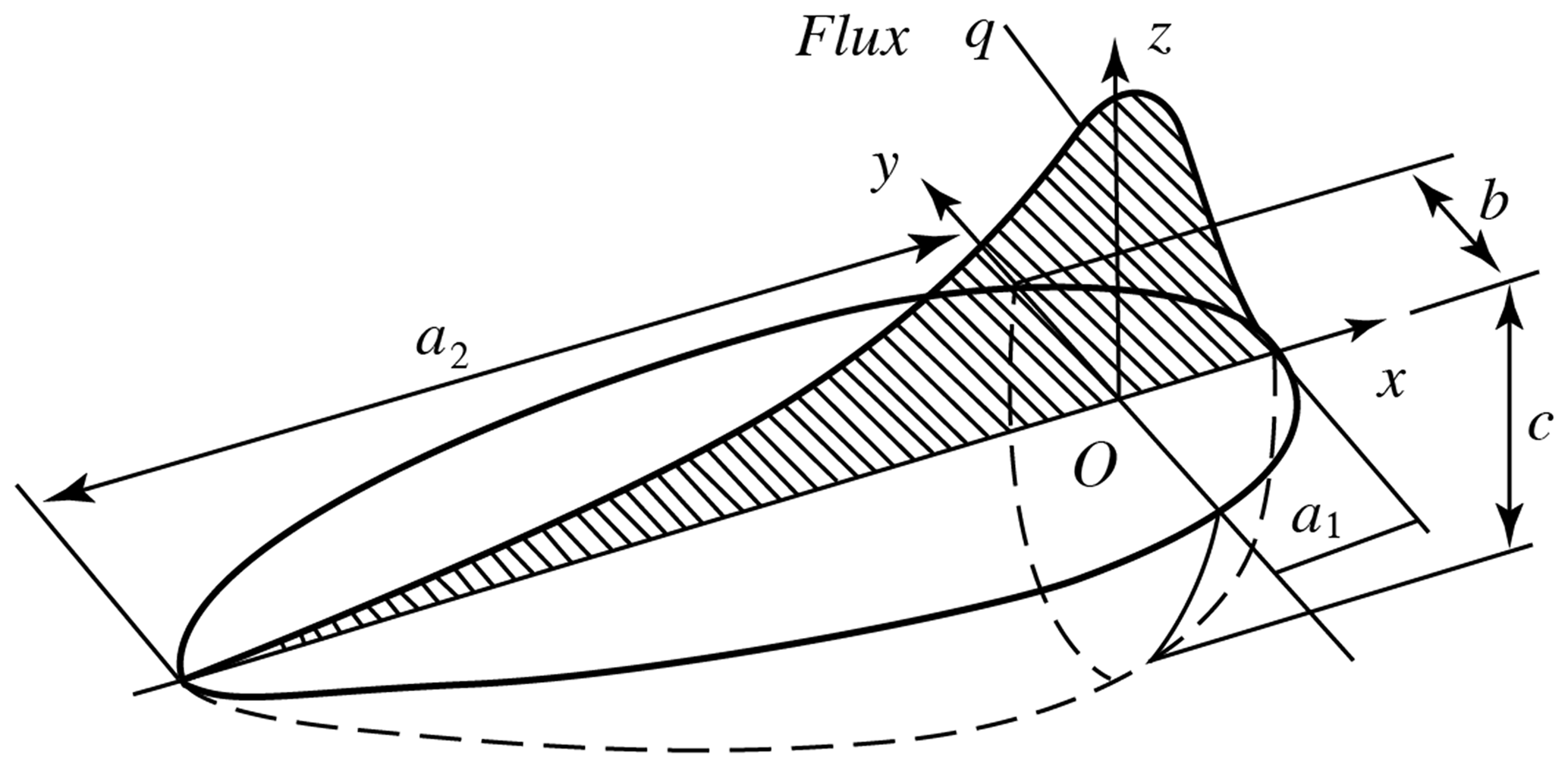
The double-ellipsoid heat source distribution model shown in Fig. 1, which can better depict the real welding pool morphology and heat source distribution under actual welding conditions, was adopted in the welding simulation (Obeid et al., 2017).
The heat flux distribution in the first semi-ellipsoid can be written as
where qf is the heat flow at point (xyz) in the first semi-ellipsoid heat source at time t, ff is the heat source partition coefficient in the first semi-ellipsoid, Q is the welding energy input rate, a1 is the half-axis length of the first semi-ellipsoid molten pool, b is the width of the molten pool, and c is the depth of the molten pool.
The heat flux distribution in the last semi-ellipsoid can be expressed as
where qr is the heat flow at point (xyz) in the last semi-ellipsoid heat source at time t, fr is the heat source partition coefficient of the last semi-ellipsoid, and a2 is the half-axis length of the last semi-ellipsoid molten pool.
If P is the welding power and η is the welding heat source efficiency, respectively, the energy input rate can be deduced as
It can be seen that the welding heat input is related to the welding heat source efficiency and welding power. According to the manual of the welding process and the geometric dimensions of the pipeline, the submerged arc welding was adopted, and the welding heat source efficiency was determined as 0.8. An ABAQUS UMAT subroutine was programmed to describe the motion of the moving heat source accurately.
2.2 Finite-element model
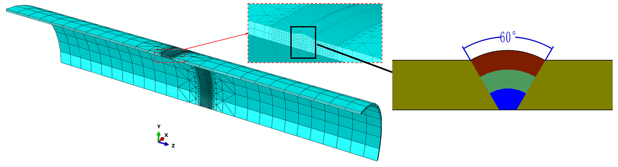
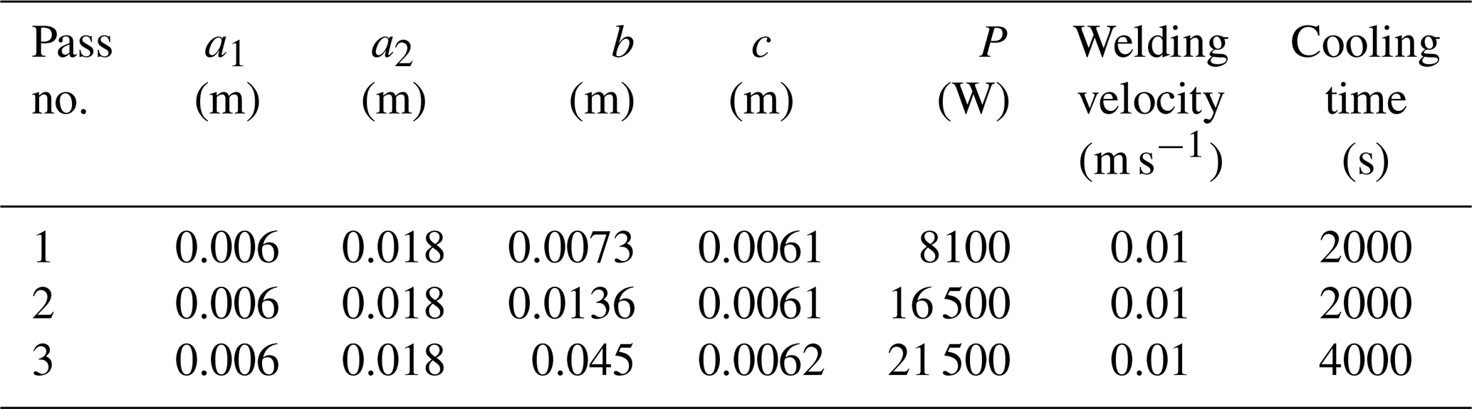
The dimensions of the welded pipeline are as follows: a diameter of 660 mm, a length of 2000 mm and a thickness of 6.4 mm. The welding finite-element model is shown in Fig. 2, the welding process is accomplished by three-pass submerged arc welding in a V-type groove (the bottom edge clearance of the V groove is 4 mm, and the groove angle is 60°), and the welding process parameters are listed in Table 1.
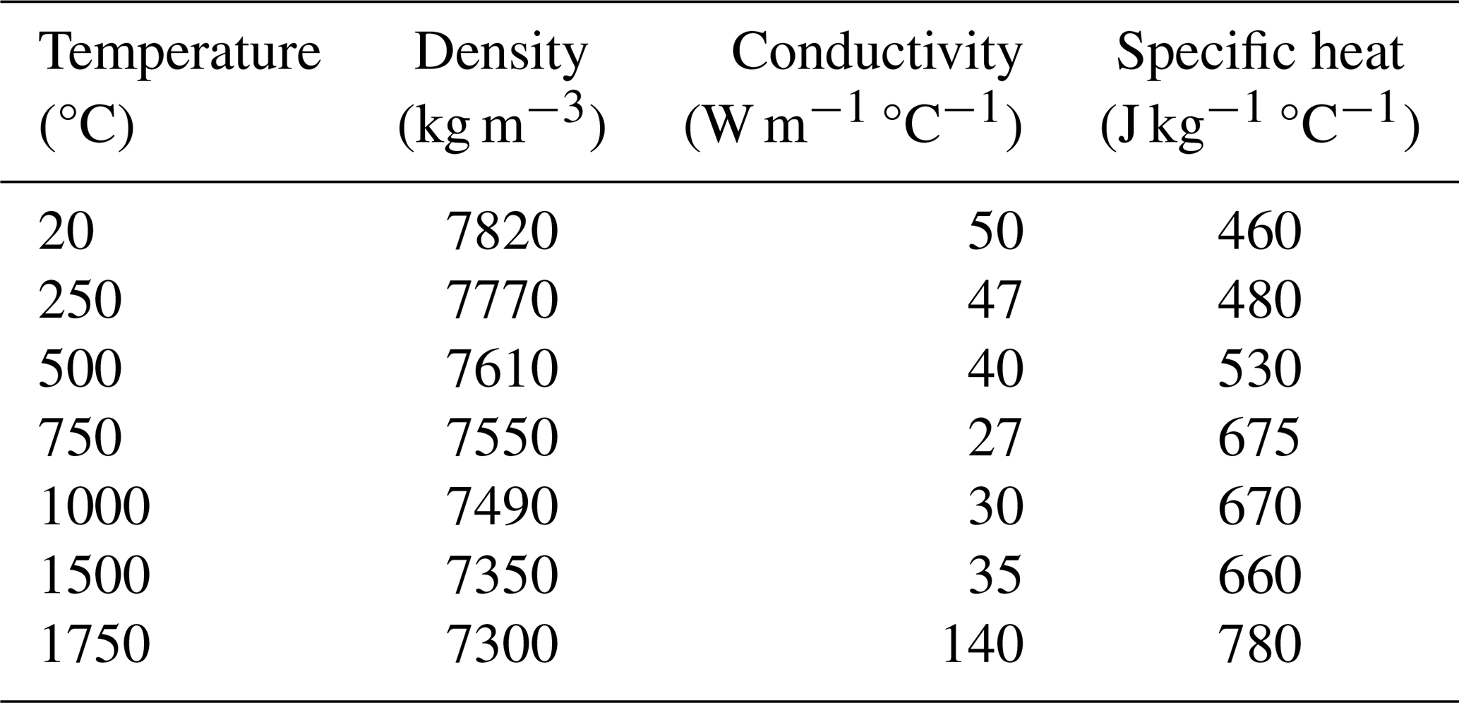
In the finite-element simulation, the welding metal and the base metal were assumed to be the same material, with the chemical compositions listed in Table 2. The thermal physical and mechanical properties are listed in Tables 3–4 (Yan et al., 2014). As can be seen, the physical and mechanical properties of X80 steel are highly dependent on the temperatures.

The governing equation of the transient heat transfer analysis during the welding process is given as
where ρ is the material density, cα is the specific heat, T is the temperature, t is the time, and λ is the thermal conductivity coefficient.
The radiation heat transfer dominates at the higher temperature near the welding seam, while convection heat transfer dominates at the surface of the welding zone with a lower temperature away from the welding zone. Therefore, the combined boundary conditions in Eq. (5) are used to apply convection and radiation to the surface of the welding zone in the form of convection by a comprehensive heat transfer coefficient H (Obeid et al., 2017), and the initial ambient temperature was set to 20 °C.
The stress–strain calculation during the welding is always based on the results of the temperature field. Generally, the welding stress may exceed the yield limit, which requires the thermal–elastoplastic theory to calculate the thermal stress accurately. In ABAQUS, the total strain rate can be decomposed and expressed as below:
where is the elastic strain rate, is the plastic strain rate, and is the thermal strain rate.
The isotropic strain-hardening model was employed to describe the initial yield and cyclic yield behavior. During the mechanical simulation, the evolution of the yield surface radius R0 was described by
where σ0 is the yield stress of the zero plastic strain, Qin and b0 are the material parameters, and is the equivalent plastic strain.
Assuming that the temperature-related mechanical properties and stress–strain vary linearly over small time increments, the stress–strain relationship in the elastic or plastic state follows
where {dσ} is the stress increment, [D] is the elastic or plastic matrix, {dε} is the strain increment, {C} is the temperature-related vector, and dT is the temperature increment.
A certain element in an elastic or plastic state has the following equilibrium equation:
where {dF}e is the force increment on the elemental node, {dR}e is the equivalent nodal force increment caused by temperature-induced initial strain, [K]e is the element stiffness matrix, and {dδ}e is the nodal displacement increment.
The finite-element-based thermal stress calculation during welding is listed as follows: when the welding temperature field is obtained, the displacement increment {dδ}e and strain increment {dε}e of each node can be calculated by adding the temperature increment gradually. According to the stress–strain relationship shown in Eq. (6), the stress increment {dσ} of each element can be obtained. In this way, the dynamic stress–strain variation and the final residual stress distribution during the entire welding process can be obtained.
2.3 Numerical results
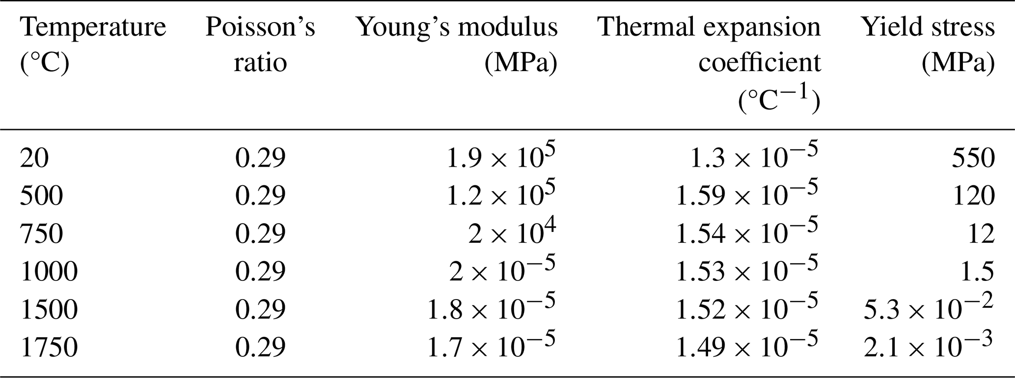
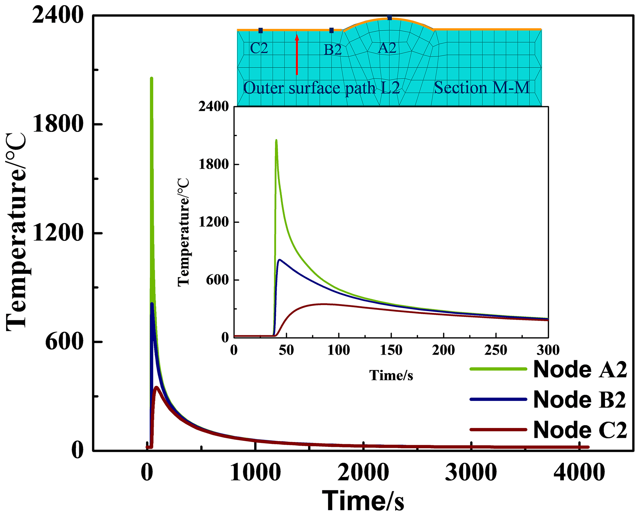
To clearly show the temperature change, path L1 at the inner surface and path L2 at the outer surface in the middle cross section M–M are selected, as shown in Fig. 3. By adjusting the welding heat source parameters, the temperature distribution of the welding molten pool can be obtained. Figure 4 demonstrates the molten pool morphology with the welding process parameters listed in Table 1. It can be found that the molten pool can melt through the welding seam, which indicates that the selected welding parameters are effective for the simulation.
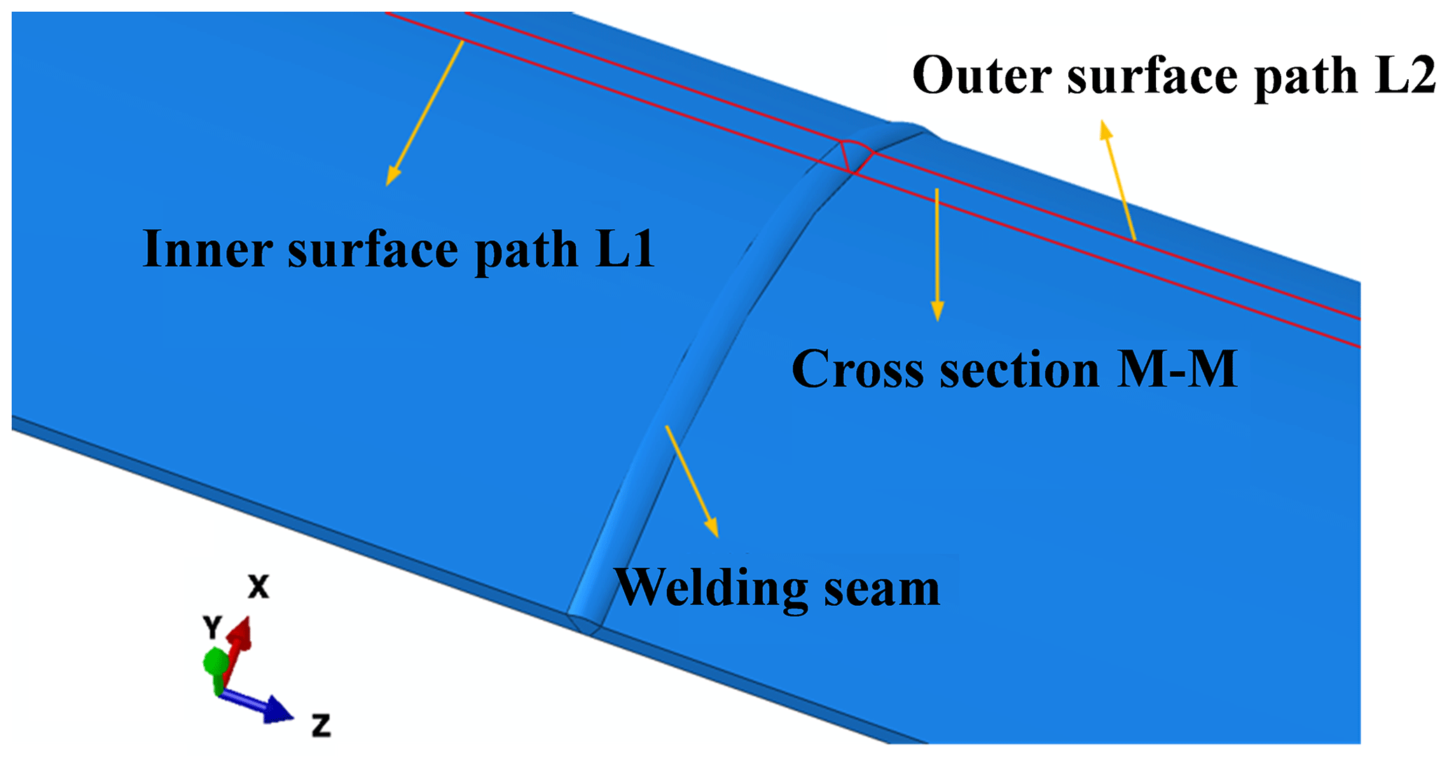
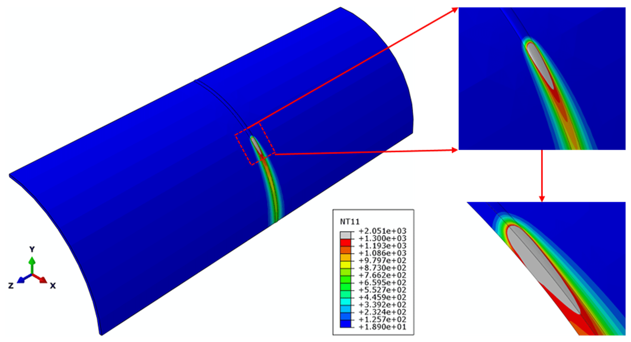
Figures 5–6 show the time-dependent temperature at different positions at paths L1 and L2 during the third-pass welding. The maximum temperature of A1 located at the center of the inner surface of the welding seam is 1326 °C. Due to the spatial distance difference, the moments when inner-surface nodes A1, B1 and C1 reach their maximum temperature are delayed successively. Node A1 is closest to the welding heat source, so node A1 has the fastest heating rate and cooling rate. After 300 s, the temperatures of A1, B1 and C1 are very close, and the temperatures cool to room temperature after 4000 s. Node A2 located at the center of the outer surface of the welding seam has a maximum temperature of 2054 °C. The temperature cycles of outer-surface nodes A2, B2 and C2 are similar to those of the inner surface nodes.
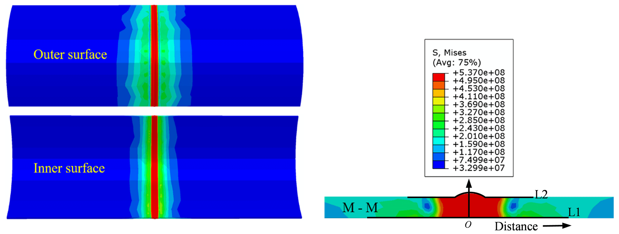
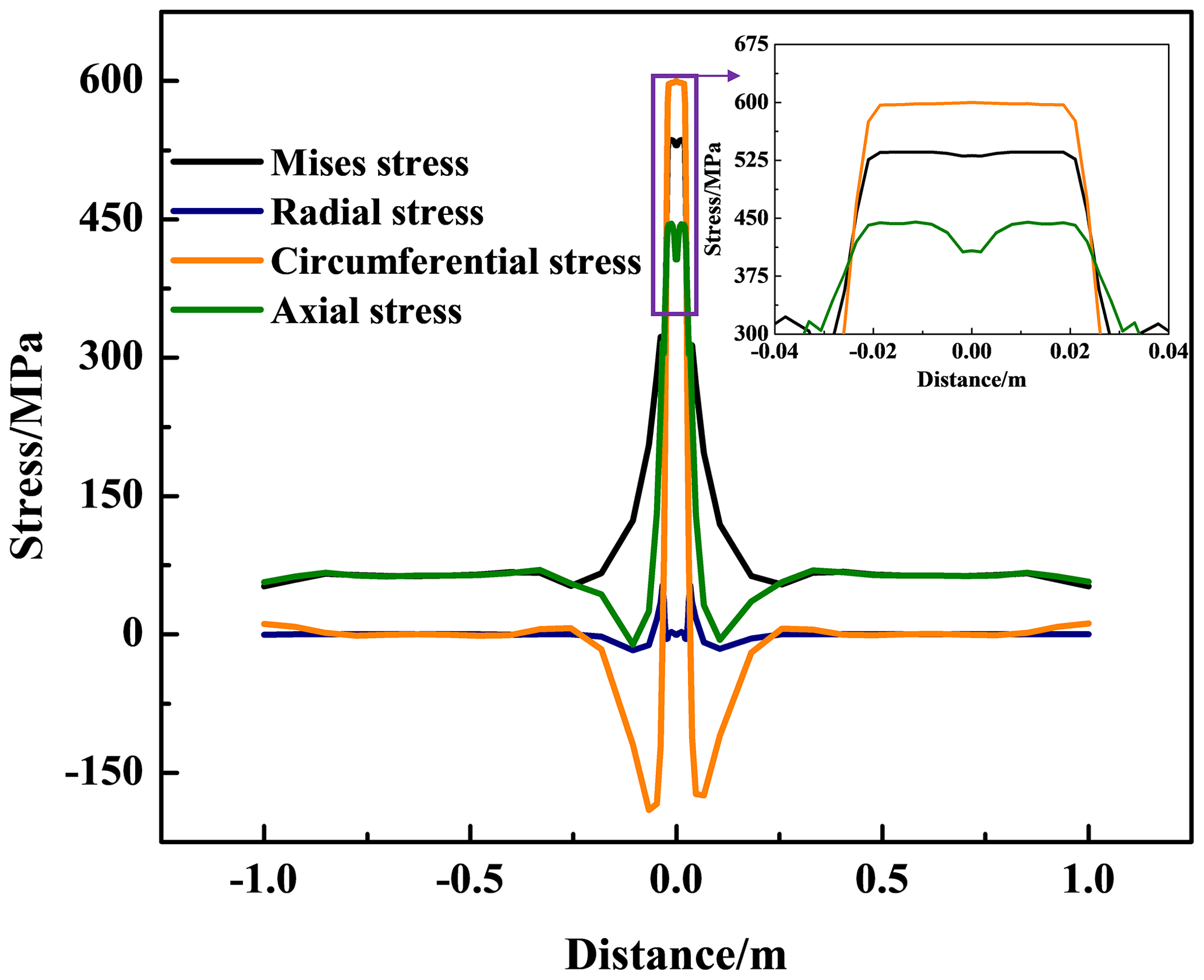
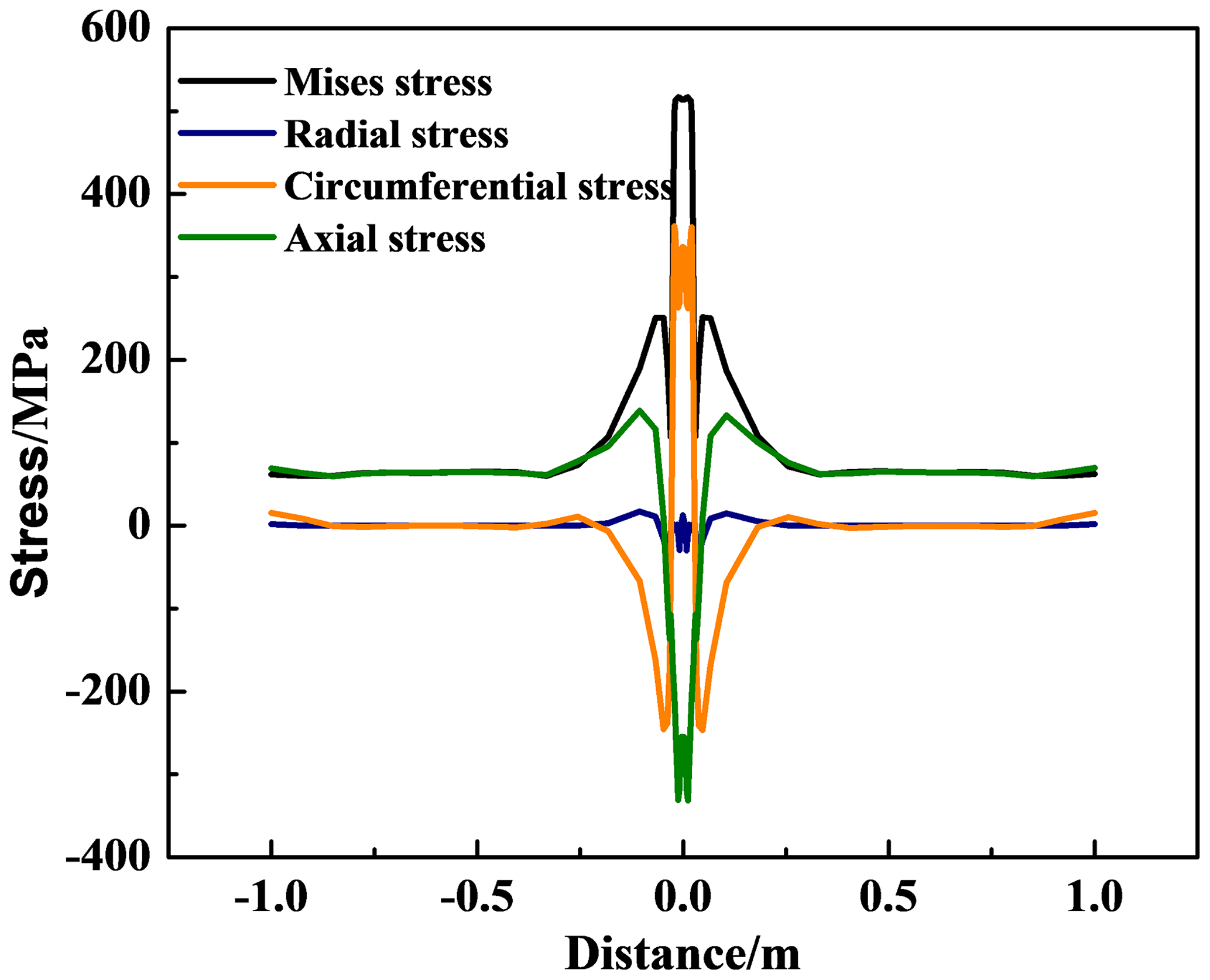
The residual stress caused by the non-uniform welding temperature was simulated using the sequential coupling method. Figure 7 shows the residual stress in the welding seam. The high Mises stress is mainly concentrated in the welding seam and HAZ, and the peak value of the residual stress is up to 537 MPa, which approaches the yield strength of the X80 steel. Figures 8–9 demonstrate the residual stresses along paths L1 and L2 at the inner and outer surfaces, respectively. The residual stress distribution at the inner surface is slightly larger than that at the outer surface. The axial stress is always in tension along path L1. However, the axial stress in the center area of the outer surface is in compression, while the axial stress quickly transforms into tensile stress outward along the welding seam.
3.1 Effect of the welding groove angle on the welding residual stress
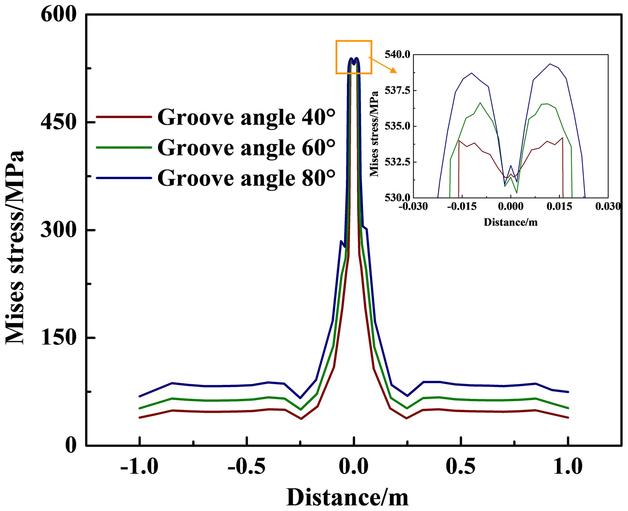
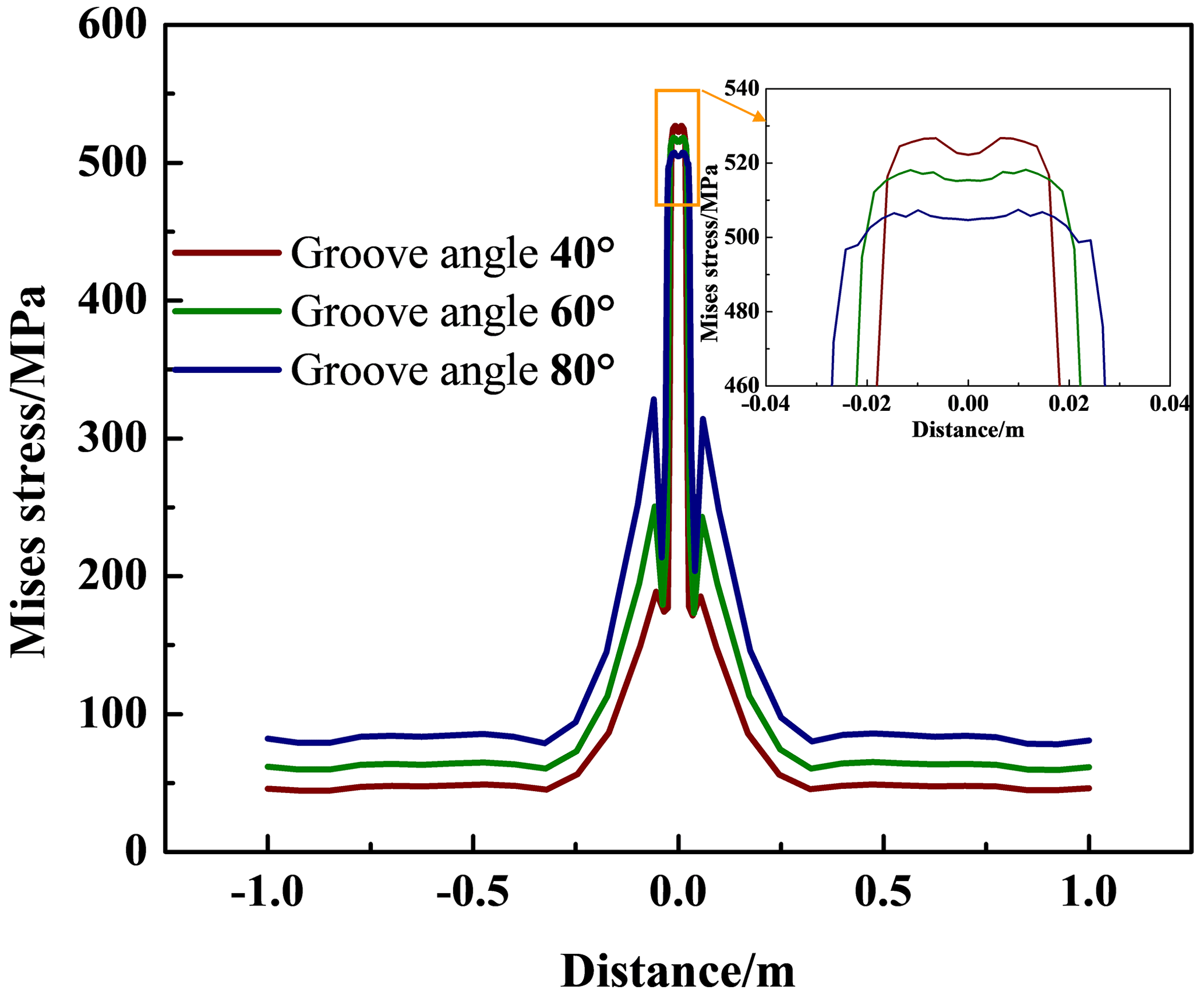
In this section, the effect of the welding groove angle on the residual welding stress is analyzed. Figure 10 demonstrates the influence of the groove angle on the residual Mises stress at the inner surface of the welding seam and the HAZ. With the increase in the welding groove angle from 40 to 80°, the residual Mises stress at the inner surface increases from 535 to 539 MPa. Figure 11 shows the influence in the groove angle on the residual Mises stress at the outer surface. With the increase in the welding groove angle, the peak Mises stress at the center of the welding seam decreases from 528 to 506 MPa, but the high-stress zone at the HAZ broadens. In general, the peak Mises stress at the outer surface is more sensitive to the change in the groove angle.
3.2 Influence of welding heat input on the welding residual stress
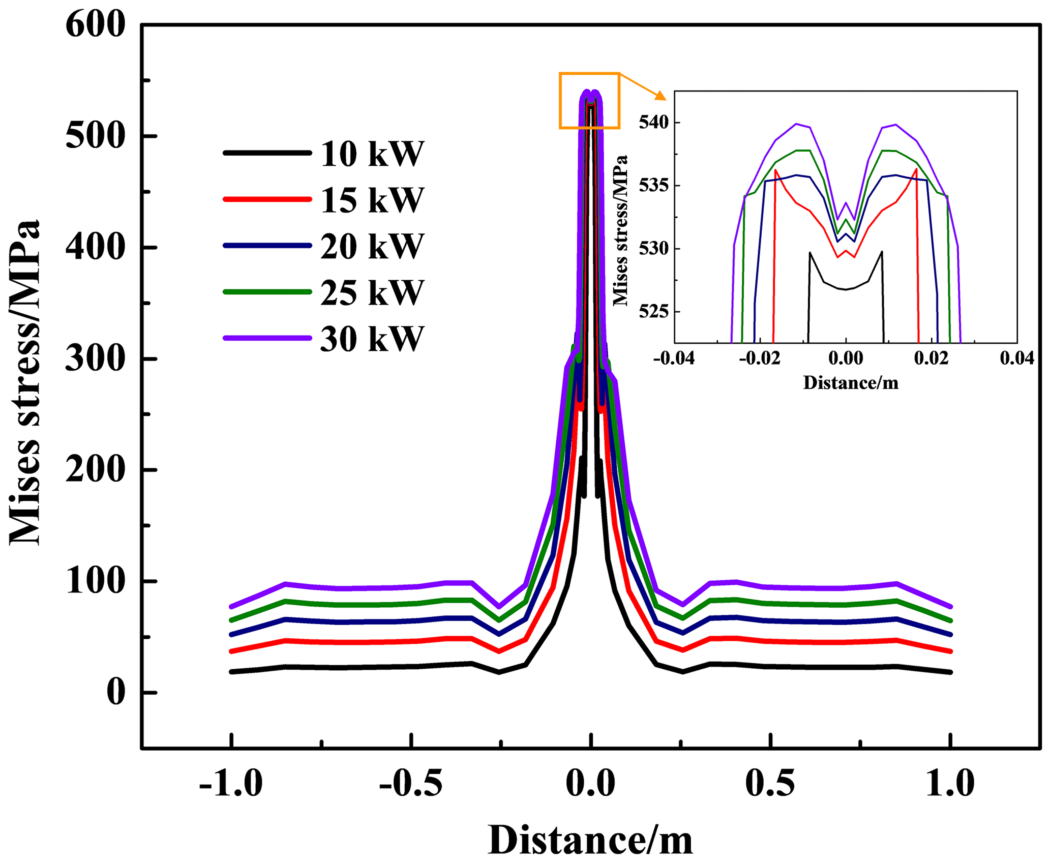
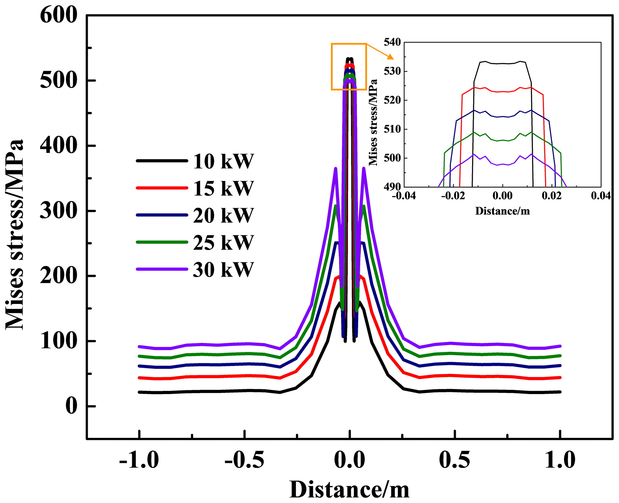
Figure 12 shows the effect of welding heat input on the Mises stress variation along path L1. As can be seen, the Mises stress at the inner surface increases with the increase in the welding heat input. Figure 13 shows the effect of welding heat input on Mises stress variation along path L2. The peak Mises stress at the center of the welding seam decreases, while the Mises stress at the HAZ increases with the increase in the welding groove angle. The influence of welding heat input on the residual Mises stress is the same as that of the welding groove angle. In the actual operation of pipeline welding, the welding process parameters can be optimized to reduce the residual welding stress.
4.1 Ultrasonic LCR wave-detecting method
To verify the effectiveness of finite-element simulation in welding residual stress, the actual X80 pipeline was welded circumferentially under the same conditions, and the residual stress of the welded pipeline was measured by the ultrasonic LCR wave-detecting method. Egle and Bray (1976) conducted extensive experiments to compare the traveling characteristics of different types of waves inside the metal material and found that the ultrasonic LCR waves have a higher sensitivity to stress than other types of ultrasonic waves.
According to the ultrasonic LCR wave-detecting method, within a fixed acoustic path L, the relationship between stress variation Δσ and acoustic traveling time difference Δt can be expressed as (Duquennoy et al., 2008)
where K is the stress coefficient in the formation
in which V0 represents the traveling velocity of the LCR wave in the zero-stress state, λ and μ are Lamé constants, and l and m are the Murnaghan constants (Akbarov, 2012).
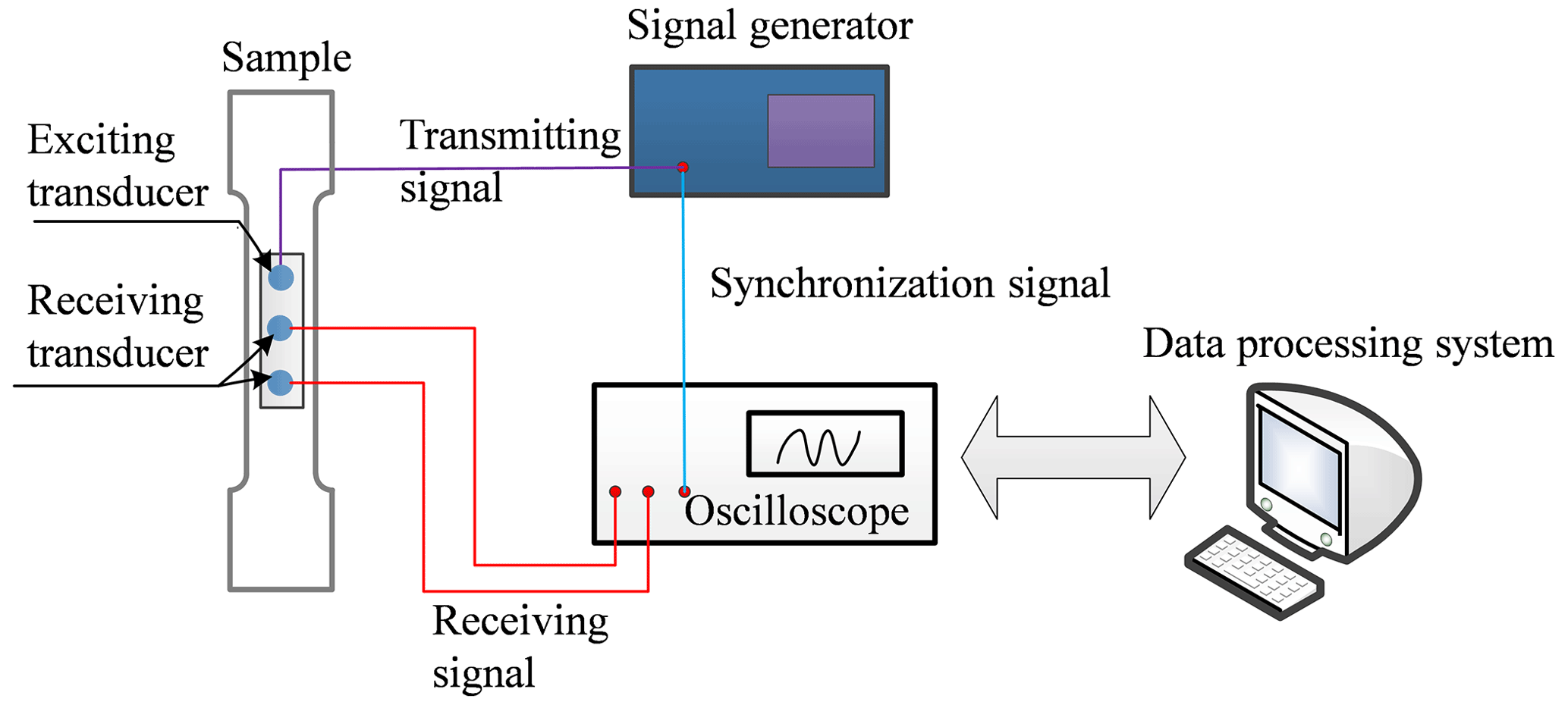
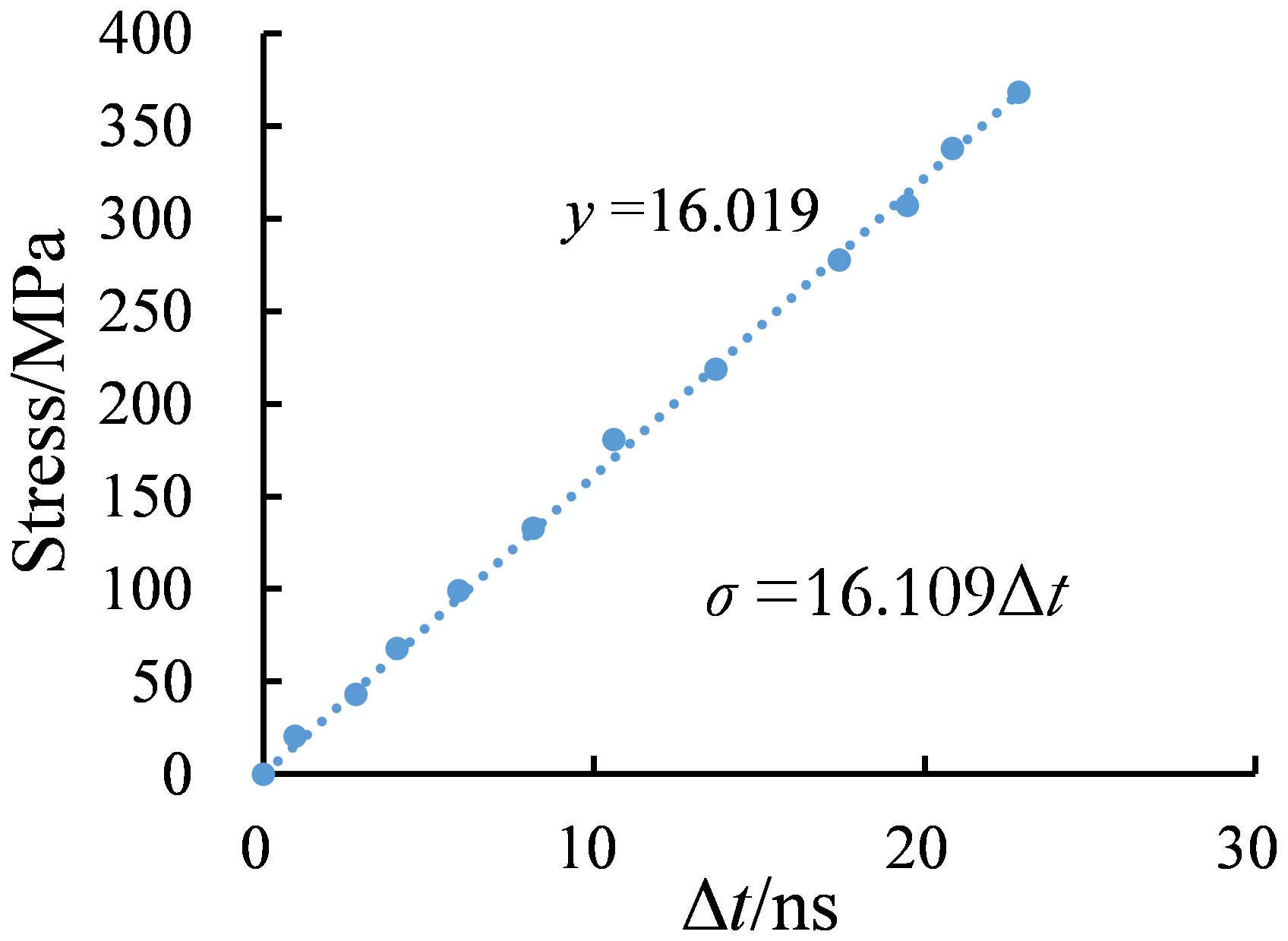
According to Eq. (8), the quantitative relationship between stress and ultrasonic LCR wave traveling time can be established under different tensile states. To measure the residual stress, it is necessary to calibrate the stress coefficient K and the traveling time of the ultrasonic LCR wave in zero stress in advance. The flow chart of the ultrasonic LCR wave stress test platform is shown in Fig. 14, and the specific implementation steps are as follows: (1) place the ultrasonic transducer probe and specimen in a constant temperature box and inject 5 mL of coupling agent onto the contact surface between the probe and specimen using a syringe; (2) when the coupling agent reaches a stable state, measure the LCR wave propagation time t0 at the zero-stress state using an online stress ultrasonic measurement system; (3) fix the X80 specimen on a universal testing machine and adjust the propagation direction of the LCR wave parallel to the direction of the loading stress; (4) load the specimen, starting from the free state until the external load stress reaches about 70 % of the yield strength, and measure the traveling time of LCR waves under the load; and (5) analyze the results of the calibration experiments and determine the stress coefficient K. According to the traveling time difference, the calibration results of the X80 steel can be obtained and are shown in Fig. 15, in which the stress coefficient K equals 16.109 MPa ns−1.
4.2 Validation of the finite-element method
The welding residual stress-detecting process of the X80 pipeline using the ultrasonic LCR wave method is shown in Fig. 16. The comparison between the stress detection and simulation results on the inner and outer surfaces of the welding seam is demonstrated in Fig. 17. Through the data analysis, the maximum error between the simulation results and test results is 26.7 %, which indicates that the welding process simulation of X80 pipelines with the finite-element method is feasible.
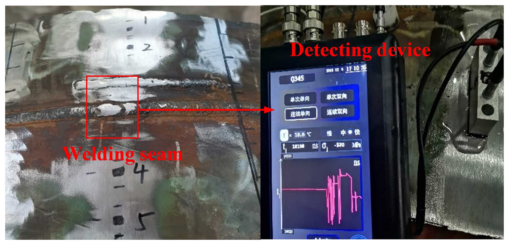
Figure 16The ultrasonic stress detection of the welding residual stress of the X80 pipeline.
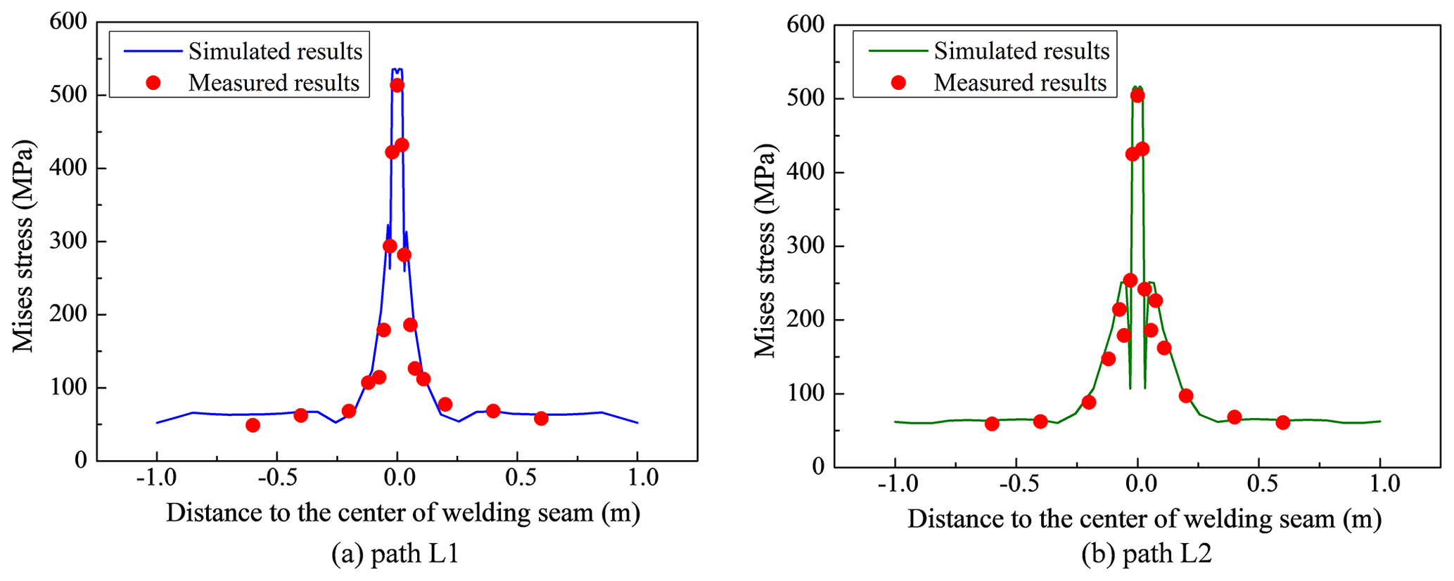
Figure 17The comparison between the stress detection and simulation results (a: path L1; b: path L2).
According to the finite-element method, the process of three-pass submerged arc welding of the X80 pipeline was simulated and the influence of welding process parameters on the welding residual stress was discussed. The ultrasonic LCR wave-detecting method was adopted to verify the finite-element simulation results. The main conclusions can be obtained as follows.
- 1.
According to the actual welding process, a moving double-ellipsoid heat source model is accomplished by an ABAQUS UMAT subroutine, and the residual stress caused by a non-uniform welding temperature is simulated using the sequential coupling method.
- 2.
Under the given welding parameters, the stress at the inner surface of the welding seam is higher than that at the outer surface, and the peak residual Mises stress is as high as 537 MPa. With the increase in the welding groove angle and heat input, the peak Mises stress increases at the inner surface and decreases at the outer surface, but the high-stress zone at the outer surface broadens. The Mises stress at the outer surface is more sensitive to the welding process parameters. Therefore, the welding process can be optimized to reduce the residual welding stress. The post-welding heat treatment is also recommended to relieve the residual stress.
- 3.
The finite-element simulation of the welding process is verified by the ultrasonic LCR wave-detecting method. According to the stress coefficient calibration and the detected results, the maximum error between the simulation results and the test results is 26.7 %, and the welding process simulation of the X80 pipeline with the finite-element method is feasible.
All the codes used in this paper can be obtained on request from the corresponding author Xiaoguang Huang (huangxg@upc.edu.cn).
All the data used in this paper can be obtained on request from the corresponding author Xiaoguang Huang (huangxg@upc.edu.cn).
ZH: conceptualization, methodology, investigation, writing – original draft. JL: data curation, writing – review and editing. LW: investigation, visualization. LL: investigation, validation. XH: conceptualization, writing – review and editing. ZY: resources, funding acquisition.
The contact author has declared that none of the authors has any competing interests.
Publisher’s note: Copernicus Publications remains neutral with regard to jurisdictional claims made in the text, published maps, institutional affiliations, or any other geographical representation in this paper. While Copernicus Publications makes every effort to include appropriate place names, the final responsibility lies with the authors.
The authors thank the reviewers for their critical and constructive review of the article.
This research has been supported by the National Natural Science Foundation of China (grant no. 11972376) and the Natural Science Foundation of Shandong Province (grant no. ZR2020ME092).
This paper was edited by Jeong Hoon Ko and reviewed by Atilla Savaş and one anonymous referee.
Akbarov, S. D.: The influence of third order elastic constants on axisymmetric wave propagation velocity in the two-layered pre-stressed hollow cylinder, CMC-Comput. Mater. Con., 32, 29–60, https://doi.org/10.1007/s11854-012-0048-9, 2012.
Chen, X., Lu, H. S., Chen, G., and Wang, X.: A comparison between fracture toughness at different locations of longitudinal submerged arc welded and spiral submerged arc welded joints of API X80 pipeline steels, Eng. Fract. Mech., 148, 110–121, https://doi.org/10.1016/j.engfracmech.2015.09.003, 2015.
Duquennoy, M., Ouaftouh, M., Devos, D., Jenot, F., and Ourak, M.: Effective elastic constants in acoustoelasticity, Appl. Phys. Lett., 92, 1145–423, https://doi.org/10.1063/ 1.2945882, 2008.
Egle, D. M. and Bray, D. E.: Measurement of acoustoelastic and third-order elastic constants for rail steel, J. Acoust. Soc. Am., 59, 741–744, https://doi.org/10.1121/1.381146, 1976.
Ferro, P.: Assessment of metallurgical and mechanical properties of welded joints via numerical simulation and experiments, Materials, 15, 3694, https://doi.org/10.3390/ma15103694, 2022.
Guo, R. B., Zhang, Y. L., Xu, X. D., Sun, L., and Yang Y.: Residual stress measurement of new and in-service X70 pipelines by X-ray diffraction method, NDT & E Int., 44, 387–393, https://doi.org/10.1016/j.ndteint.2011.03.003, 2011.
Javadi, Y. and Najafabadi, M. A.: Comparison between contact and immersion ultrasonic method to evaluate welding residual stresses of dissimilar joints, Mater. Design, 47, 473–482, https://doi.org/10.1016/j.matdes.2012.12.069, 2013.
Katsuyama, J., Tobita, T., Itoh, H., and Onizawa, K.: Effect of welding conditions on residual stress and stress corrosion cracking behavior at Butt-welding joints of stainless steel pipes, J. Press. Vess.-T. ASME, 134, 021403, https://doi.org/10.1115/1.4005391, 2012.
Mendez, P. F., Tello, K. E., and Lienert, T. J.: Scaling of coupled heat transfer and plastic deformation around the pin in friction stir welding, Acta Mater., 58, 6012–6026, https://doi.org/10.1016/j.actamat.2010.07.019, 2010.
Obeid, O., Alfano, G., and Bahai, H.: Thermo-mechanical analysis of a single-pass weld overlay and girth welding in lined pipe, J. Mater. Eng. Perform., 26, 3861–3876, https://doi.org/10.1007/s11665-017-2821-5, 2017.
Park, J. H., Kim, D. S., Cho, D. W., Kim, J., and Pyo, C.: Influence of thermal flow and predicting phase transformation on various welding positions, Heat Mass Transfer, 60, 195–207, https://doi.org/10.1007/s00231-023-03429-w, 2023.
Peng, Y., Zhao, J., Chen, L. S., and Dong, J.: Residual stress measurement combining blind-hole drilling and digital image correlation approach, J. Constr. Steel Res., 176, 106346, https://doi.org/10.1016/j.jcsr.2020.106346, 2021.
Savaş, A.: Investigating the thermal and structural responses in hard-facing application with the GTAW process, J. Theor. App. Mech.-Pol., 59, 343–353, https://doi.org/10.15632/jtam-pl/136210, 2021a.
Savaş, A.: Selection of welding conditions for minimizing the residual stresses and deformations during hard-facing of mild steel, Brodogradnja, 72, 1–18, https://doi.org/10.21278/brod72101, 2021b.
Singh, M. P., Arora, K. S., Kumar, R., Shukla, D. K., and Prasad, S. S.: Influence of heat input on microstructure and fracture toughness property in different zones of X80 pipeline steel weldments, Fatigue Fract. Eng. M., 44, 85–100, https://doi.org/10.1111/ffe.13333, 2021.
Sirohi, S., Kumar, N., Kumar, A., Pandey, S. M., Adhithan, B., Fydryvh, D., and Pandey, C.: Metallurgical characterization and high-temperature tensile failure of Inconel 617 alloy welded by GTAW and SMAW-a comparative study, P. I. Mech. Eng. L-J. Mat., 237, 2046–2067, https://doi.org/10.1177/14644207231171266, 2023.
Tangestani, R., Farrahi, G. H., Shishegar, M., Aghchehkandi, B. P., Ganguly, S., and Mehmanparast, A.: Effects of vertical and pinch rolling on residual stress distributions in wire and arc additively manufactured components, J. Mater. Eng. Perform., 29, 2073–2084, https://doi.org/10.1007/s11665-020-04767-0, 2020.
Vemanaboina, H., Edison, G., and Akella, S.: Effect of residual stresses of GTA welding for dissimilar materials, Mater. Res., 21, e20171053, https://doi.org/10.1590/1980-5373-MR-2017-1053, 2018.
Vemanaboina, H., Akella, S., Uma Maheshwer Rao, A., Gundabattini, E., and Buddu, R. K.: Analysis of thermal stresses and its effect in the multipass welding process of SS316L, P. I. Mech. Eng. E-J. Pro., 235, 384–391, https://doi.org/10.1177/0954408920965062, 2021.
Wang, K., Jiao, X. D., Zhu, J. L., Li, J. Y., and Li, C. W.: Research on the effect of weld groove on the quality and stability of laser-MAG hybrid welding in horizontal position, Weld. World, 65, 1701–1709, https://doi.org/10.1007/s40194-021-01125-z, 2021.
Wang, X., Liao, B., Wu, D. Y., Han, X. L., Zhang, Y. S., and Xiao, F. R.: Effects of hot bending parameters on microstructure and mechanical properties of weld metal for X80 hot bends, J. Iron Steel Res. Int., 21, 1129–1135, https://doi.org/10.1016/S1006-706X(14)60194-1, 2014.
Yan, C. Y., Liu, C. Y., and Yan, B.: 3D modeling of the hydrogen distribution in X80 pipeline steel welded joints, Comp. Mater. Sci., 83, 158–163, https://doi.org/10.1016/j.commatsci.2013.11.007, 2014.
Yang, Y. H., Shi, L., Xu, Z., Lu, H. S., Chen, X., and Wang, X.: Fracture toughness of the materials in welded joint of X80 pipeline steel, Eng. Fract. Mech., 148, 337–349, https://doi.org/10.1016/j.engfracmech.2015.07.061, 2015.
Zhang, F. L., Liu, S. Y., Liu, F. D., Liu, R., and Zhang, H.: Effect of groove angle and heat treatment on the mechanical properties of high-strength steel hybrid laser-MAG welding joints, Mater. Res. Express, 6, 1265g1, https://doi.org/10.1088/2053-1591/ab6776, 2019.
Zhao, W. M., Jiang, W., Zhang, H. J., Han, B., Jin, H. C., and Gao, Q.: 3D finite element analysis and optimization of welding residual stress in the girth joints of X80 steel pipeline, J. Manuf. Process., 66, 166–178, https://doi.org/10.1016/j.jmapro.2021.04.009, 2021.