Irrigation, damming, and streamflow fluctuations of the Yellow River

Yin, Zun; Ottlé, Catherine; Ciais, Philippe; Zhou, Feng; Wang, Xuhui; Jan, Polcher; Dumas, Patrice; Peng, Shushi; Li, Laurent; Zhou, Xudong; Bo, Yan; Xi, Yi; Piao, Shilong

doi:https://doi.org/10.5194/hess-25-1133-2021

Articles | Volume 25, issue 3

https://doi.org/10.5194/hess-25-1133-2021

Articles | Volume 25, issue 3

Research article

05 Mar 2021

Research article |

| 05 Mar 2021

Irrigation, damming, and streamflow fluctuations of the Yellow River

Zun Yin, Catherine Ottlé, Philippe Ciais, Feng Zhou, Xuhui Wang, Polcher Jan, Patrice Dumas, Shushi Peng, Laurent Li, Xudong Zhou, Yan Bo, Yi Xi, and Shilong Piao

Abstract

The streamflow of the Yellow River (YR) is strongly affected by human activities like irrigation and dam operation. Many attribution studies have focused on the long-term trends of streamflows, yet the contributions of these anthropogenic factors to streamflow fluctuations have not been well quantified with fully mechanistic models. This study aims to (1) demonstrate whether the mechanistic global land surface model ORCHIDEE (ORganizing Carbon and Hydrology in Dynamic EcosystEms) is able to simulate the streamflows of this complex rivers with human activities using a generic parameterization for human activities and (2) preliminarily quantify the roles of irrigation and dam operation in monthly streamflow fluctuations of the YR from 1982 to 2014 with a newly developed irrigation module and an offline dam operation model. Validations with observed streamflows near the outlet of the YR demonstrated that model performances improved notably with incrementally considering irrigation (mean square error (MSE) decreased by 56.9 %) and dam operation (MSE decreased by another 30.5 %). Irrigation withdrawals were found to substantially reduce the river streamflows by approximately $242.8 \pm 27.8 \times 10^{8}$ m³ yr⁻¹ in line with independent census data ( $231.4 \pm 31.6 \times 10^{8}$ m³ yr⁻¹). Dam operation does not change the mean streamflows in our model, but it impacts streamflow seasonality, more than the seasonal change of precipitation. By only considering generic operation schemes, our dam model is able to reproduce the water storage changes of the two large reservoirs, LongYangXia and LiuJiaXia (correlation coefficient of ∼ 0.9). Moreover, other commonly neglected factors, such as the large operation contribution from multiple medium/small reservoirs, the dominance of large irrigation districts for streamflows (e.g., the Hetao Plateau), and special management policies during extreme years, are highlighted in this study. Related processes should be integrated into models to better project future YR water resources under climate change and optimize adaption strategies.

Download & links

Article (PDF, 3598 KB)

Supplement (210 KB)

Download & links

Article (3598 KB)
Supplement (210 KB)
BibTeX
EndNote

How to cite

How to cite.

Dates

Received: 08 Jan 2020 – Discussion started: 16 Apr 2020 – Revised: 05 Jan 2021 – Accepted: 10 Jan 2021 – Published: 05 Mar 2021

1 Introduction

More than 60 % of all rivers in the world are disturbed by human activities (Grill et al., 2019), contributing altogether to approximately 63 % of surface water withdrawal (Hanasaki et al., 2018). River water is used for agriculture, industry, drinking water supply, and electricity generation (Hanasaki et al., 2018; Wada et al., 2014), these usages being influenced by direct anthropogenic drivers and by climate change (Haddeland et al., 2014; Piao et al., 2007, 2010; Yin et al., 2020; Zhou et al., 2020). In order to meet the fast-growing water demand in populated areas and to control floods (Wada et al., 2014), reservoirs have been built for regulating the temporal distribution of river water (Biemans et al., 2011; Hanasaki et al., 2006), leading to a massive perturbation of the seasonality and year-to-year variations of streamflows. In the midlatitude–northern latitude regions, where a decrease of rainfall is observed historically and projected by climate models (IPCC, 2014), water scarcity will be further exacerbated by the growth of water demand (Hanasaki et al., 2013) and by the occurrence of more frequent extreme droughts (Seneviratne et al., 2014; Sherwood and Fu, 2014; Zscheischler et al., 2018). Thus, adapting river management is a crucial question for sustainable development, which requires comprehensive understanding of the impacts of human activities on river flow dynamics,, particularly in regions under high water stress (Liu et al., 2017; Wada et al., 2016).

The Yellow River (YR) is the second longest river in China. It flows across arid, semi-arid, and semi-humid regions, and the catchment contains intensive agricultural zones and has a population of 107 million inhabitants (Piao et al., 2010). With 2.6 % of total water resources in China, the Yellow River basin (YRB) irrigates 9.7 % of the croplands (http://www.yrcc.gov.cn, last access: 28 February 2021). Underground water resources are used in the YRB, but they only account for 10.3 % of total water resources, outlining the importance of streamflow water for regional water use. A special feature of the YRB is the huge spatiotemporal variation of its water balance. Precipitation is concentrated in the flooding season (from July to October) which constitutes ∼ 60 % of the annual discharge, whereas the dry season (from March to June) represents only ∼ 10 %–20 %. Numerous dams have been built to regulate the streamflows intra- and inter-annually in order to control floods and alleviate water scarcity (Liu et al., 2015; Zhuo et al., 2019). The YRB streamflows are thus highly controlled by human water withdrawals and dam operations, making it difficult to separate the impacts of human and natural factors on the variability and trends.

Numerous studies documented the effects of anthropogenic factors on streamflows and water resources in the YRB by statistical approaches (e.g., Liu and Zhang, 2002; Jin et al., 2017; Miao et al., 2011; Wang et al., 2006, 2018; Zhuo et al., 2019). To further elucidate the mechanisms, physical-based land surface hydrology models including natural and anthropogenic factors are required. Many previous model studies only considered natural processes, and YRB simulations were evaluated against naturalized streamflows (Liu et al., 2020; Xi et al., 2018; Yuan et al., 2018; Zhang and Yuan, 2020). YRB modeling studies simulating real streamflows and comparing their values to observed streamflows are scarce, the most important being from Jia et al. (2006) and Tang et al. (2008). Yet, Jia et al. (2006) prescribed census irrigation and dam operation data as input of their model. Tang et al. (2008) included irrigation as a mechanism in their DBH (distributed biosphere hydrological) model and investigated the long-term trends of streamflows, but they described the irrigation demand simply from satellite leaf area data, so that crop plant water requirements and phenology were not represented by physical laws. Several global hydrological models (GHMs) simulated both irrigation and dam operation processes and were applied for future projection of water resources regionally (Liu et al., 2019) or globally (Hanasaki et al., 2018; Wada et al., 2014, 2016). Those global GHM studies acknowledged the complex situation of the YRB where models' performances are limited, but none has focused on the sources of error or potential overlooked mechanisms in this catchment.

To model present water resources in the YRB and make future projections, not only natural mechanisms, but also anthropogenic ones must be represented in a model. If a key mechanism is missing in a model, a calibration of its parameters to match observations can compensate for structural biases, and projections may be erroneous. For example, the HBV model (Hydrologiska Byråns Vattenbalansavdelning) was well calibrated with different approaches in 156 catchments in Austria but failed in predicting streamflow changes due to climate warming (Duethmann et al., 2020), one of the key reasons being that the response of vegetation to climate change was missing in the model. In this study, we integrate two key anthropogenic processes (irrigation and dam operation) in the land surface model ORCHIDEE (ORganizing Carbon and Hydrology in Dynamic EcosystEms), which has a mechanistic description of plant–climate and soil water availability interactions and of river streamflows. Through a set of simulations with generic parameter values, we aim to preliminarily diagnose how irrigation and dam operation improve the simulations of observed YRB streamflows. After making sure we understand the impact of adding these two new and crucial processes, the model will be calibrated against a suite of observations so that it can be applied for future projections.

Using a standard version of ORCHIDEE without irrigation or dams, Xi et al. (2018) performed simulations with a 0.1^∘ hypo-resolution atmospheric forcing over China (Chen et al., 2011). They attributed the trends of several river streamflows to natural drivers from increased CO₂ and climate change and to land use change. Lacking irrigation and other human removals, their simulated results were higher than the observed streamflows for the YRB. By developing a crop module in ORCHIDEE (Wang et al., 2016; Wang, 2016; Wu et al., 2016), ORCHIDEE was able to provide precise estimation of crop physiology, phenology, and yield at both local and national scales, as well as other site-based crop models, e.g., EPICs (Folberth et al., 2012; Izaurralde et al., 2006; Liu et al., 2007, 2016; Williams, 1995), CGMS-WOFOST (de Wit and van Diepen, 2008), APSIM (Elliott et al., 2014; Keating et al., 2003), and DSSAT (Jones et al., 2003), and land surface models, e.g., CLM-CROP (Drewniak et al., 2013), LPJ-GUESS (Smith et al., 2001; Lindeskog et al., 2013), LPJmL (Waha et al., 2012; Bondeau et al., 2007), and PEGASUS (Deryng et al., 2011, 2014; Wang et al., 2017; Müller et al., 2017). ORCHIDEE-estimated irrigation accounts for potential ecological and hydrological impacts (e.g., physiological response of plants to climate change and short-term drought episodes on soil hydrology) with respect to other land surface models (LSMs) and GHMs (Hanasaki et al., 2008; Leng et al., 2015; Thiery et al., 2017; Nazemi and Wheater, 2015; Voisin et al., 2013). In a study focusing on China (Yin et al., 2020), ORCHIDEE was able to simulate irrigation withdrawals across China and to evaluate them against census data with a provincial-based spatial correlations of ∼ 0.68. It successfully explained the decline of total water storage in the YRB. In this study, we add a simple module describing the dam operations to further improve the model over the YRB.

A simple dam operation model is developed and firstly coupled to ORCHIDEE to simulate the real streamflows in this study. Similar to other GHMs and LSMs, our dam operation model is based on generic operation principles due to a lack of related data. Recent dam models are developed from different perspectives, such as the agent-based model River Wave (Humphries et al., 2014), the basin-specific model Colorado River Simulation System (Bureau of Reclamation, 2012), and the original dam module in the Variable Infiltration Capacity (VIC) model (Lohmann et al., 1998). However, the representation of dam operations in many global hydrological studies (e.g., Droppers et al., 2020; Haddeland et al., 2006, 2014; Hanasaki et al., 2018; Zhao et al., 2016; Yassin et al., 2019; Wada et al., 2014, 2016) is based on the ideas of Hanasaki et al. (2006). They categorized dams based on their regulation purposes (irrigation and non-irrigation). Irrigation-oriented rules adjust the dam retention to meet the irrigation demand downstream, while non-irrigation-oriented rules buffer floods and thus dampen the variability (Hanasaki et al., 2006). However, the water release target of a dam in the model of Hanasaki et al. (2006) is fixed at the beginning of the year and cannot adjust interactively to large intra- and inter-annual climate variations, which is a key feature of the YRB. To overcome this limitation, we propose a new dam operation model based on a target operation plan, constrained by the regulation capacity of a dam and historical simulated streamflows, with flexibility to adjust to climate variation. The effects of dams on streamflows could then be studied with ORCHIDEE and isolated from the effect of climate factors and irrigation demands. Different from classical approaches separating the YRB into an upper, middle, and lower stream (Tang et al., 2008; Zhuo et al., 2019), here we further divide both the upper and middle streams into sub-catchments based on the locations of five key gauging stations (Fig. 1). This approach splits regions with and without big dams (or large irrigation areas) in the upper and middle streams, which simplifies the assessment of the effects of irrigation and damming on streamflows.

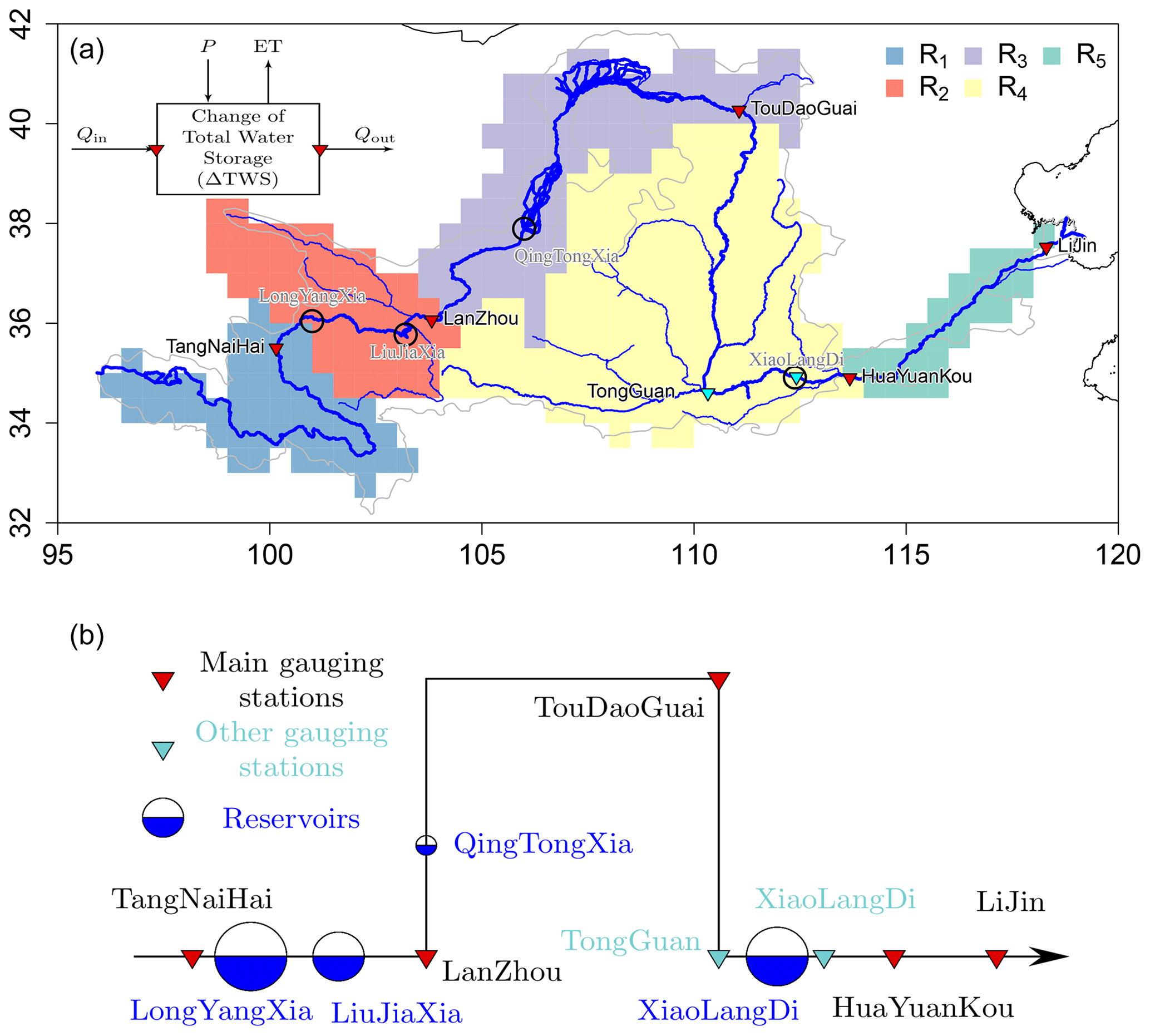
https://hess.copernicus.org/articles/25/1133/2021/hess-25-1133-2021-f01

Figure 1(a) Map of YRB. Gray and blue lines indicate the catchment and network of YR based on GIS data, respectively. Dark circles are main artificial reservoirs on the YR. Triangles are gauging stations. Red triangles are main stations used for classifying sub-catchment and simulation comparison, and teal triangles are stations used to assess the impacts of XiaoLangDi Reservoir on river streamflows. Colored patterns are sub-catchments between two neighboring gauging stations based on the ORCHIDEE routing map. The water balances of specific sub-catchments are shown in the top left. (b) Conceptual figure of YR main stream, gauging stations, and artificial reservoirs. The sizes of circles indicate the regulation capacities of these reservoirs (Table 2).

In this study, ORCHIDEE, with the novel crop–irrigation module (Wang, 2016; Yin et al., 2020) and the new dam operation model, was applied in the YRB from 1982 to 2014 in order to (1) demonstrate whether ORCHIDEE and the dam model, with generic parameterizations, are able to improve the simulation of streamflow fluctuations and (2) attempt to separate the effect of irrigation and dams on the fluctuations of monthly streamflows. We first describe the ORCHIDEE model and our new dam model in Sect 2.1. Then we present the algorithm used for estimating sub-catchment water balances in Sect. 2.2, followed by the input and evaluation datasets, the simulation protocol, and metrics for evaluation in Sect. 2.3 to 2.5. Results are presented in Section 3, and limitations are discussed in Sect. 4.

2 Methodology

2.1 ORCHIDEE land surface model used in this study

2.1.1 Irrigation and crop modules

ORCHIDEE is a physical process-based land surface model that integrates the hydrological cycle, surface energy balances, the carbon cycle, and vegetation dynamics using two main modules. The SECHIBA (surface–vegetation–atmosphere transfer scheme) module simulates the dynamics of the water cycle, energy fluxes, and photosynthesis at a 0.5 h time interval, which are used by the STOMATE (Saclay Toulouse Orsay Model for the Analysis of Terrestrial Ecosystems) to estimate vegetation and soil carbon cycle at daily time step. The ORCHIDEE model used in this study is a special version with a newly developed crop and irrigation module (Wang et al., 2017; Wu et al., 2016; Yin et al., 2020). The crop module includes specific parameterizations for wheat, maize, and rice, calibrated over China using observations (Wang, 2016; Wang et al., 2017). It is able to simulate crop carbon allocation and different phenological stages, as well as related management (e.g., planting date, rotation, multi-cropping, and irrigation).

Irrigation amount is simulated in the land surface model ORCHIDEE (Wang, 2016; Wang et al., 2017) as the minimum between crop water requirements and the water supply. The crop water requirements are defined according to the choice of irrigation technique, namely minimizing soil moisture stress for the flooding technique, sustaining plant potential evapotranspiration for the dripping technique, and maintaining the water level above the soil surface during specific months for the paddy irrigation technique. Each crop is grown on a specific soil column (in each model grid cell), where the water and energy budgets are independently resolved. The water resources in the hydrological routing scheme are from three water reservoirs: (1) a streamflow component, (2) a fast reservoir with surface runoff, and (3) a slow reservoir with deep drainage, used in this order for defining the priorities of water use for irrigation. As long-distance water transfer is not modeled, streams only supply water to the crops growing in the grid cell they cross, according to the river routing scheme of the ORCHIDEE model (Ngo-Duc et al., 2007). Without dams, irrigation can be underestimated where dams store water to supply the crop demand. Transfer from reservoirs, lakes, or local ponds to adjacent cells is not considered, which should further lead to an underestimation of the irrigation supply, dependent on the cell size. Details of the coupled crop–irrigation module of ORCHIDEE are described in Yin et al. (2020).

2.1.2 New dam operation model

To account for the impacts of dam regulation on streamflow (Q) seasonality, we developed a dynamic dam water storage module based on only two generic rules: reducing flood peaks and guaranteeing base flow. This model depends on simulated inflows and is thus independent from irrigation demands. It has been developed for the main reservoirs of the YRB (e.g., the LongYangXia, LiuJiaXia, and XiaoLangDi in Fig. 1). Different from Biemans et al. (2011) and Hanasaki et al. (2006), we primarily consider the ability of reservoirs to regulate river flow seasonality. This means that the target base flow and flood control of our dam model are not fixed proportions of the mean annual streamflow but depend on the regulation capacity of the reservoir (C_max). Firstly, similar to Voisin et al. (2013), a multi-year averaged monthly streamflow (Q_s) is calculated based on ORCHIDEE simulations. To include the potential impacts of recent climate change on dam operation, here we only consider the latest past 10-year simulations, as

\begin{matrix} (1) & Q_{s, i} = \frac{1}{N} \sum_{j}^{j \in N} Q_{i}^{j} . \end{matrix}

Here Q_s,i (m³ s⁻¹) is the multi-year averaged monthly streamflow of month i; j is the year index; and N is the number of years accounted for. For an upcoming year j, we only use the historical simulations (maximum latest 10 years) to calculate Q_s.

Secondly, we evaluate the target water storage change ΔW_t and monthly streamflow Q_t considering the regulation capacity of each reservoir. As shown in Fig. S1 in the Supplement, 1 year can be divided into two periods by comparing Q_s with ${\overline{Q}}_{s}$ . The longest continuous period of months with $Q_{s} > {\overline{Q}}_{s}$ is the recharging season for reservoirs, and the rest is the releasing season. The amount of water stored during the recharging season (blue region in Fig. S1) is determined by C_max and is used during the releasing season (red regions in Fig. S1). The values of ΔW_t and Q_t can be estimated by

\begin{array}{l} (2) & k = min (\frac{C_{max}}{α \sum_{i}^{i \in Recharge} Q_{s, i}}, k_{max}), \\ (3) & Δ W_{t, i} = α [k (Q_{s, i} - {\overline{Q}}_{s}) + {\overline{Q}}_{s}], \\ (4) & Q_{t, i} = Q_{s, i} - Δ W_{t, i} / α . \end{array}

Here k (–), varying between 0 and k_max (=0.7), indicates the ability of the reservoir to disturb streamflow seasonality. It is a ratio of the maximum regulation capacity of the reservoir C_max (10⁸ m³) over the streamflow amount throughout the recharging season. α (0.0263) converts monthly streamflow to water volume. Assuming that the water storage of the reservoir reaches C_max at the end of the recharging season, we can calculate target water storage W_t by using ΔW_t.

Finally, the variation of the actual water storage of the reservoir ΔW is a decision regarding actual monthly streamflow, current water storage, Q_t, ΔW_t, and W_t. During the releasing season, ΔW is calculated as

\begin{matrix} (5) & \begin{array}{ll} - W_{i} \frac{(- Δ W_{t, i})}{W_{t, i}} & if W_{i} \leq W_{t, i}; \\ Δ {\tilde{W}}_{i} - [(W_{i} + Δ {\tilde{W}}_{i}) - (W_{t, i} + Δ W_{t, i})] & if W_{i} > W_{t, i} and Δ {\tilde{W}}_{i} > Δ W_{t, i}; \\ Δ W_{t, i} - (W_{i} - W_{t, i}) & if W_{i} > W_{t, i} and Δ {\tilde{W}}_{i} \leq Δ W_{t, i} . \end{array} \end{matrix}

$Δ {\tilde{W}}_{i} = α Q_{i} - (α Q_{t, i} - Δ W_{t, i})$ . It is the expected release amount to make river streamflows equal to the target streamflows after reservoir regulation. If current water storage is less than the target value (the case of Eq. 5), the ΔW_i is calculated by the W_i with a proportion of ΔW_t,i over W_t,i. If the current storage is more than the target value (the cases of Eq. 5), the reservoir can release more water based on a balance between the target water storage change ΔW_t,i and the target water storage at the next time step W_t,i (represented by $Δ {\tilde{W}}_{i}$ ). Note that all water storage change variables are negative throughout the releasing season.

During the recharging season, we can calculate the ΔW_i as

\begin{matrix} (6) & \begin{array}{ll} max (min (W_{t, i} + Δ W_{t, i} - W_{i}, α Q_{i}), 0) & if W_{i} > W_{t, i}; \\ min (Δ W_{t, i} + (W_{t, i} - W_{i}), α Q_{i}) & if W_{i} \leq W_{t, i} . \end{array} \end{matrix}

If current water storage is larger than the target value (Eq. 6), we will try to recharge a volume of water to make $W_{i + 1} = W_{t, i + 1}$ . If current water storage is less than the target value (Eq. 6), we decide to recharge additional water volume besides the ΔW_t,i.

ΔW is then applied as a correction of simulated streamflows to generate actual monthly streamflows using the following equation:

\begin{matrix} (7) & {\hat{Q}}_{sim, i} = Q_{sim, i} - \frac{1}{α} Δ W_{i} . \end{matrix}

Here ${\hat{Q}}_{sim}$ (m³ s⁻¹) is the simulated regulated streamflows, and Q_sim (m³ s⁻¹) is the simulated monthly streamflows. Note that this model is a simplified representation of dam management because it ignores the direct coupling between water demand and irrigation water supply from the cascade of upstream reservoirs. This approach implies that, with a regulated flow, demands will be able to be satisfied and floods avoided without being more explicit. A complete coupling of demand, flood, and reservoir management is difficult to implement in the land surface model in the absence of data about the purpose and management strategy of each dam, given different possibly conflicting demands of water for industry and drinking versus cropland irrigation.

Before performing the simulation, we estimate the maximum regulation capacity of each studied reservoir in each river sub-catchment shown in Fig. 1. Table 1 lists collected information of the main reservoirs on the YR. Only large reservoirs like LongYangXia (LYX), LiuJiaXia (LJX), and XiaoLangDi (XLD) are considered in our model because of their huge C_max.

Table 1Information of artificial reservoirs on the YR with considerable total capacity. Data are mainly from the YR Conservancy Commission of the Ministry of Water Resources (http://www.yrcc.gov.cn, last access: 28 February 2021). The “regulation purposes” follow the style of Hanasaki et al. (2006). “H” indicates hydropower; “C” indicates flood control; “I” indicates irrigation; “W” indicates water supply; and “S” indicates scouring sediment.

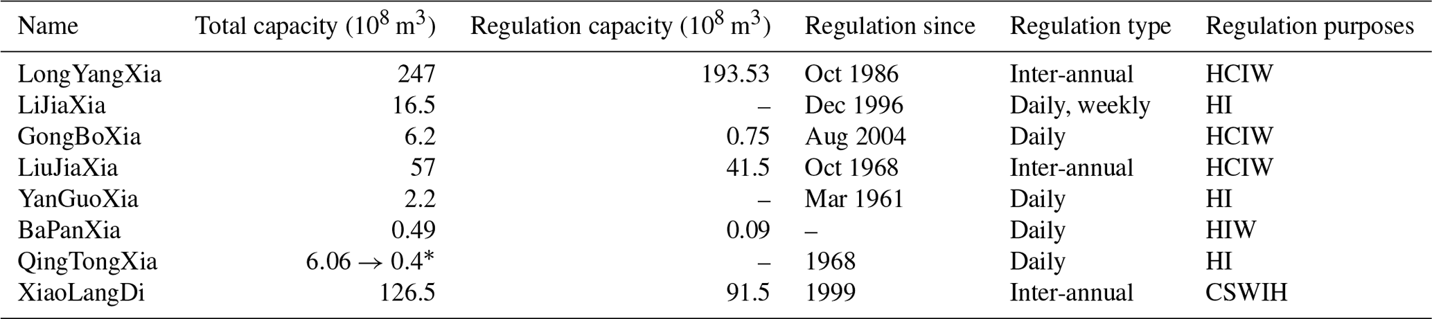
^* The total capacity shrink is due to sedimentation.

Download Print Version | Download XLSX

2.2 Sub-catchment diagnosis

Figure 1 shows the YRB and main gauging stations used in this study. To effectively use Q_obs for investigating impacts of irrigation and dam regulations on the streamflows of different river sub-catchments, we divided the YRB into five sub-catchments (R_i, $i \in [1, 5]$ ; Fig. 1) with an outlet at each gauging station. Thus we can evaluate the water balance in R_i by

\begin{matrix} (8) & \frac{Δ {TWS}_{i}}{Δ t} = P_{i} - {ET}_{i} + \frac{Q_{in, i} - Q_{out, i}}{A_{i}}, \end{matrix}

where Δt is the time interval, ΔTWS_i (mm) is the change of total water storage in specific R_i, P_i (mm Δt⁻¹) is precipitation in R_i, ET_i (mm Δt⁻¹) is evapotranspiration in R_i, and A_i (m²) is the area of R_i. Q_in,i and Q_out,i (m³ Δt⁻¹) are inflow and outflow respectively. In addition, $q_{i} = Q_{out, i} - Q_{in, i}$ indicates the contribution of R_i to the river streamflows, that is the sub-catchment streamflows. This term can be negative if local water supply (e.g., precipitation and groundwater) cannot meet water demand. A conceptual figure of the water balance of a sub-catchment is shown in the top left of Fig. 1.

2.3 Evaluation datasets

Observed monthly streamflows (Q_obs) from the gauging stations shown in Fig. 1 are used to evaluate the simulations. Several precipitation (P) and evapotranspiration (ET) datasets were selected to evaluate the simulated water budgets in each sub-catchment of the YRB. The 0.5^∘ 3-hourly precipitation data from GSWP3 (Global Soil Wetness Project Phase 3) used as model input are based on GPCC v6 (Global Precipitation Climatology Centre; Becker et al., 2013) after bias correction with observations. The MSWEP (Multi-Source Weighted-Ensemble Precipitation) is a 0.25^∘ 3-hourly P product integrating numerous in situ measurements, satellite observations, and meteorological reanalysis (Beck et al., 2017). Three ET datasets are chosen for their potential ability to capture the effect of irrigation disturbance on ET (Yin et al., 2020) (noted as ET_obs). GLEAM v3.2a (Global Land Evaporation Amsterdam Model; Martens et al., 2017) provides 0.25^∘ daily ET estimations based on a two-soil layer model in which the top soil moisture is constrained by the ESA CCI (European Space Agency Climate Change Initiative) Soil Moisture observations. The FLUXCOM model (Jung et al., 2009) upscales ET data from a global network of eddy covariance tower measurements into a global 0.5^∘ monthly ET product. Since these towers do not cover irrigated systems, ET from irrigation simulated by the LPJmL (Lund–Postam–Jena managed Land) is added to ET from non-irrigated systems. The PKU ET product estimates 0.5^∘ monthly ET using water balances at basin scale, integrating FLUXNET observations to diagnose sub-basin patterns using a model tree ensemble approach (Zeng et al., 2014).

2.4 Simulation protocol

The 0.5^∘ half-hourly GSWP3 atmospheric forcing (Kim, 2017) was used to drive ORCHIDEE simulations. Yin et al. (2018) used four atmospheric forcing datasets to drive ORCHIDEE to simulate soil moisture dynamics over China, and they found that the GSWP3 provided the best performances; hence we chose this forcing for this study. A 0.5^∘ map with 15 different plant functional types (PFTs) containing crop sowing area information for the three PFTs corresponding to the modeled crop (wheat, maize, and rice) is used, based on a 1:1 million vegetation map and provincial-scale census data of China. Crop planting dates for wheat, maize, and rice are derived from the spatial interpolation of phenological observations from the Chinese Meteorological Administration (Wang et al., 2017). The soil texture map is from Zobler (1986). Two simulation experiments were performed to assess the impacts of irrigation on streamflows: (1) NI, no irrigation, and (2) IR, irrigated by available water resources. In IR, only surface irrigation is considered, that is, water applied on the cropland soil without interception by canopies. The soil water stress, a function of soil moisture and crop root density up to 2 m depth (Yin et al., 2020), is checked every half an hour. When it is less than a target threshold, irrigation is triggered with an amount equal to the difference between saturated and current soil moisture. To precisely estimate irrigation water consumption (direct water loss from the surface water pool excluding return flow), deep drainage of the three crop soil columns is turned off in the IR simulation. Simulations start from a 20-year spin-up in 1982 to initialize the thermal and hydrological variables then continued from 1982 to 2014. A validation against naturalized streamflows is shown in the Supplement Table S1.

Table 2Definitions of sub-catchments and values of C_dam used in the dam regulation simulation.

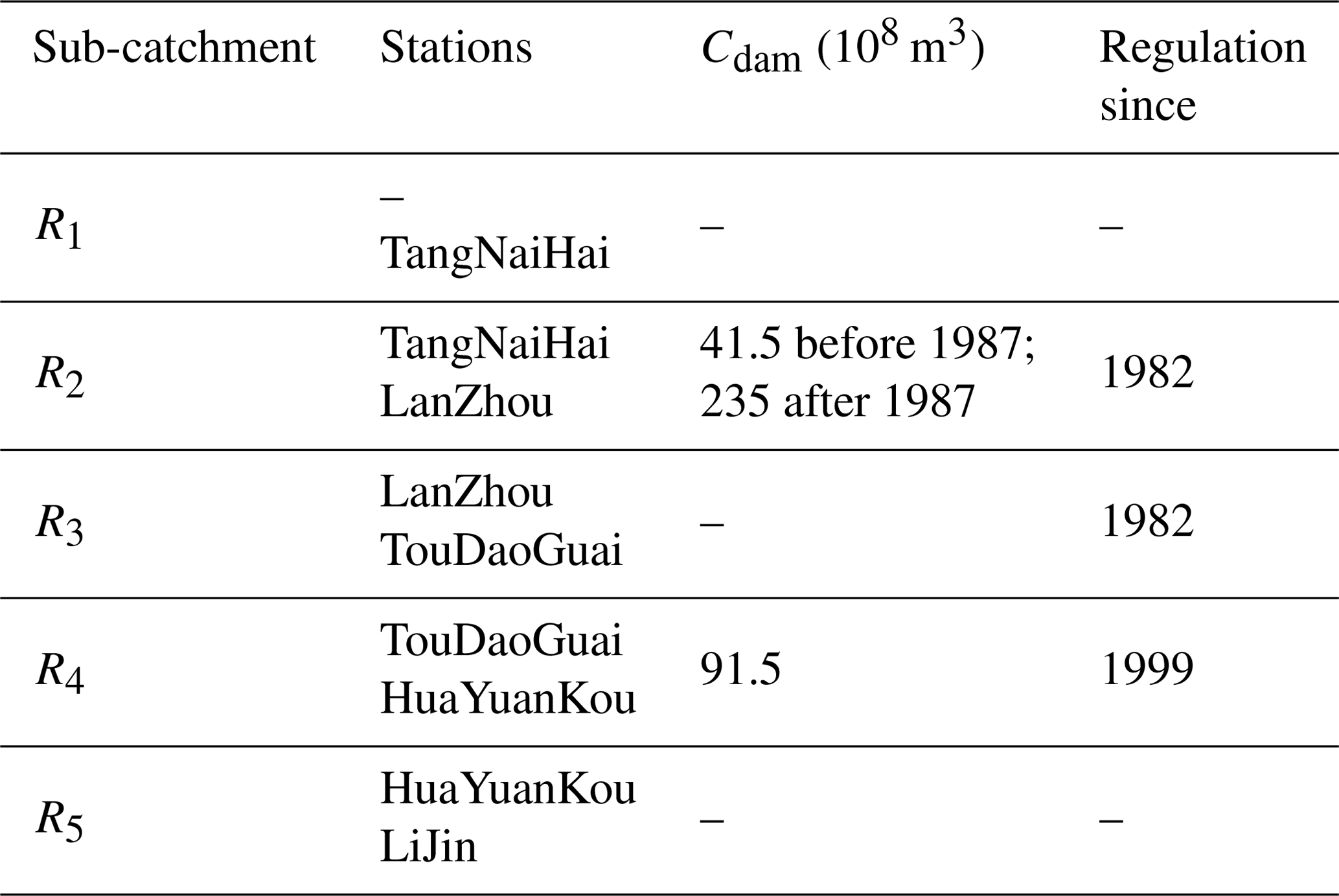
Download Print Version | Download XLSX

The dam operation simulation starts from 1982 as an offline model applied to the simulated streamflows from the IR simulation (Q_IR) as input. The initial values of W were set to half of the C_max. Considering the potential joint regulation of reservoirs, we firstly estimate the total ΔW of all considered reservoirs by using Q_IR at HuaYuanKou (outlet of R₄; Fig. 1). Then we estimate the ΔW of LYX and LJX reservoir by using Q_IR at LanZhou. The difference between these two ΔW is assumed to be the ΔW of the XLD reservoir in between. Offline simulated ΔW values are used to estimate regulated monthly streamflows ( ${\hat{Q}}_{IR}$ ) as in Eq. (7). As huge irrigation water withdrawals occur in R₃ and R₅ (YRCC, 2014), the water recharge of reservoirs may result in negative ${\hat{Q}}_{IR}$ at TouDaoGuai and LiJin. To avoid this numerical artifact due to the offline nature of our dam model, we corrected all negative ${\hat{Q}}_{IR}$ to zero by assuming that the streamflows cannot further drop when all stream water is consumed upstream. The impact of these corrections is accounted for at gauging stations downstream to ensure mass conversation.

2.5 Evaluation metrics

Three metrics are used to evaluate the performances of simulated monthly Q. The mean square error (MSE) evaluates the magnitude of errors between simulation and observations. It can be decomposed into three components (Kobayashi and Salam, 2000):

\begin{matrix} (9) & MSE = \frac{1}{n} \sum_{i = 1}^{n} {(S_{i} - O_{i})}^{2} = SB + SDSD + LCS, \end{matrix}

where S_i and O_i are simulated and observed values, respectively, and n is the number of samples. SB (squared bias) is the bias between simulated and observed values. In this study, SB represents the difference between simulated and observed multi-year mean annual Q. SDSD (the squared difference between standard deviation) relates to the mismatch of variation amplitudes between simulated and measured values. It can reflect whether our simulation can capture the seasonality of Q_obs. LCS (the lack of correlation weighted by the standard deviation) indicates the mismatch of fluctuation patterns between simulated and observed values, which is equivalent to inter-annual variation of Q in this study. The formulas of these three components and a detailed explanation can be found in Kobayashi and Salam (2000).

The index of agreement ( $d \in [0, 1]$ ) is defined as the ratio of MSE and potential error. It is calculated as

\begin{matrix} (10) & d = 1 - \frac{\sum_{i = 1}^{n} {(O_{i} - S_{i})}^{2}}{\sum_{i = 1}^{n} {(| S_{i} - \overline{O} | + | O_{i} - \overline{O} |)}^{2}}, \end{matrix}

where d=1 indicates perfect fit, and d=0 denotes poor agreement.

The modified Kling–Gupta efficiency ( $mKGE \in (- \infty, 1]$ ) is defined as the Euclidean distance of three independent criteria: correlation coefficient r, bias ratio β, and variability ratio γ (Gupta et al., 2009; Kling et al., 2012). It is an improved indicator from the Nash–Sutcliffe efficiency avoiding heterogeneous sensitivities to peak and low flows, which is crucial for this study that is not only interested in simulating peak flows but also concentrates on base flows regulated by dams for human usage. The mKGE is calculated as

\begin{matrix} (11) & mKGE = 1 - \sqrt{(1 - r)^{2} + (1 - β)^{2} + (1 - γ)^{2}}, \\ (12) & β = \frac{μ_{S}}{μ_{O}}; γ = \frac{{CV}_{S}}{{CV}_{O}}, \end{matrix}

where r is the correlation coefficient between observed and simulated streamflows, and μ (m³ s⁻¹) and CV (–) are the mean and the coefficient of variation of Q, respectively. These indicators are used for three comparisons: (1) Q_NI and Q_obs, (2) Q_IR and Q_obs, and (3) ${\hat{Q}}_{IR}$ and Q_obs.

https://hess.copernicus.org/articles/25/1133/2021/hess-25-1133-2021-f02

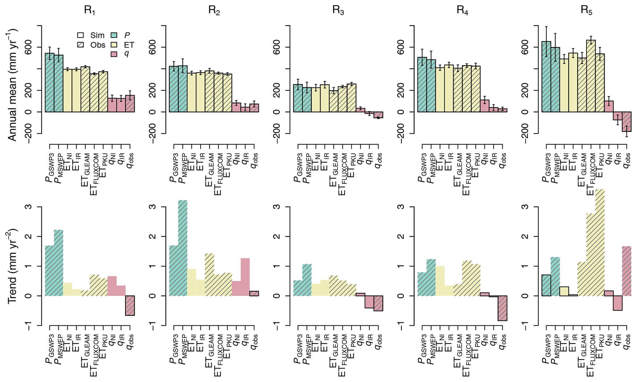
Figure 2Top panels: annual mean of hydrological elements in each sub-catchment of the YR basin from both simulation (plain colors) and observation (hatched colors). Error bars represent standard deviation. Bottom panels: trends of these elements in each sub-catchment. Dark borders indicate the trend is statistically significant (p-value <0.05) according to the Mann–Kendall test.

Download

3 Results

3.1 Water budgets at sub-catchment scale

Figure 2 displays water budgets and trends in R_i based on simulation and observations. Going from upstream to downstream, precipitation in P_GSWP3, which is consistent with P_MSWEP, decreases from 543.6 mm yr⁻¹ (R₁) to 254.2 mm yr⁻¹ (R₃) and then rises again to 652.1 mm yr⁻¹ (R₅). The magnitudes of simulated ET (both ET_NI and ET_IR) have no significant differences with ET_obs aggregated over sub-catchments R₁ to R₅. Grid-cell-based validation shows high agreement between simulated and observed ET across all sub-catchments. The lowest mean of correlation coefficients is 0.79, and the highest mean of relative root mean square error (RMSE) is 4.9 % (Table S2). Except for R₁ where cropland is rare, ET_IR accounts for an amount representing more than 80 % of P_GSWP3 in the YRB, with a maximum value of 96.5 % in R₃. The difference between ET_IR and ET_NI is due to the irrigation process, which accounts for 9.1 % and 8.2 % of ET_NI in R₃ and R₅ respectively as caused by the irrigation demand. The impact of irrigation can be detected from sub-catchment streamflows ( $q_{i} = (Q_{out, i} - Q_{in, i}) / A_{i}$ ) as well. For instance, both q_obs and q_IR are negative in R₃ and R₅, suggesting that local surface water resources cannot meet water demand for irrigation. As irrigation water transfers between grid cells are not represented in our simulations, the non-availability of water locally results in an underestimation of the irrigation withdrawals, likely explaining why q_IR>q_obs in R₃ to R₅.

The trends of P and ET are positive but not significant in most R_i during the period 1982–2014 (bottom panels of Fig. 2). However, significant trends can be found in simulated and observed q in some R_i. The decrease of q_obs in R₁ is not captured by the model, neither in q_NI nor q_IR. This underestimated decrease of river streamflows might be linked to decreased glacier melt or increased non-irrigation-related human water withdrawals, which are ignored in our simulations. In R₂ and R₃, the q_obs trends are determined by the joint effects of climate change (e.g., the P increase) and human water withdrawals. The trends of q_IR show the same direction as those of q_obs. In R₅, however, q_obs increased by 1.67 mm yr⁻¹, which was not captured by our simulation of q_IR. Besides the increase of P, another possible driver of increasing q_obs in R₅ is a decrease of water withdrawal due to the improvement of irrigation efficiency (Yin et al., 2020), which is not accounted for in our simulations. Moreover, water use management may play an important role in the observed positive trends of q_obs as well, with the aim to increase the streamflows downstream of the YR to avoid streamflow cutoff (Q_obs<1 m³ s⁻¹) that occurred in the 1990s (Wang et al., 2006).

Irrigation not only influences annual streamflows in the YR but also affects its intra-annual variation. In general, the discharge yield Y_Q, defined by the sum of surface runoff and drainage, of all grid cells in NI should be higher than in IR because our irrigation model can remove water from the stream reservoirs which is a fraction of drainage and runoff. However, our simulations show that Y_Q,NI can be less than Y_Q,IR (Fig. S2) at the beginning of the monsoon season. This is because irrigation keeps soil moisture higher than without irrigation in July in R₄ and R₅ (Fig. S2d and e), which in turn promotes Y_Q because the soil water-holding capacity is lower, and a larger fraction of P can go to runoff. This mechanism highlighted that irrigation could enhance the heterogeneity of water temporal distribution and may reinforce floods after a dry season.

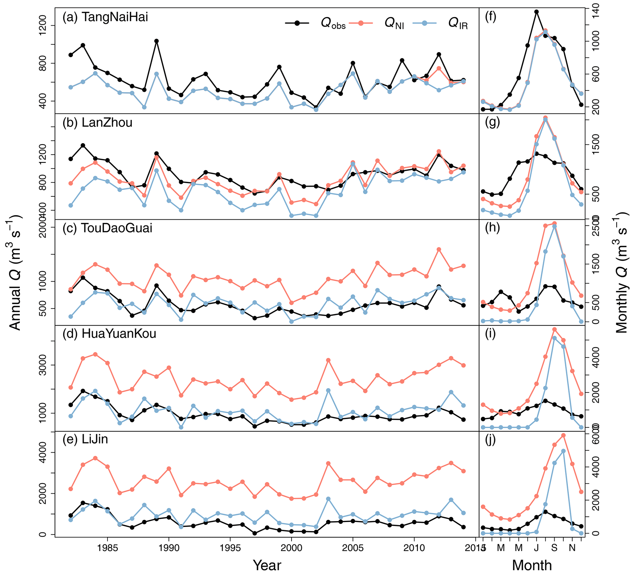
https://hess.copernicus.org/articles/25/1133/2021/hess-25-1133-2021-f03

Figure 3(a–e) Time series of annual streamflows from observations and simulations at each gauging station. (f–j) Seasonality of observed and simulated streamflows at each gauging station. Q_obs is the observed annual mean streamflows. Q_NI and Q_IR are the simulated annual mean streamflows based on the NI and IR simulations (Sect. 2.4), respectively. These simulations do not account for dams, and therefore the seasonality has a higher amplitude than observed in the plots on the right-hand side.

Download

3.2 Comparison between observed and simulated Q

Figure 3 shows time series of annual streamflows and of the seasonality of monthly streamflows. Our simulations underestimate Q_obs at TangNaiHai in R₁, likely because we miss glacier melt. After LanZhou, the values of Q_IR coincide very well with those of Q_obs, indicating that irrigation strongly reduces the annual streamflows of the YR. However, the seasonality of monthly Q_IR is different from Q_obs (Fig. 3f–j). Despite the good match of annual values, the model without dams (shown in Fig. 3) produces an underestimation of Q in the dry season and an overestimation of Q in the flood season. Such a mismatch of Q seasonality is likely caused primarily by dam regulation ignored in the model. The locations of several big reservoirs are shown in Fig. 1b, and their characteristics are listed in Table 1.

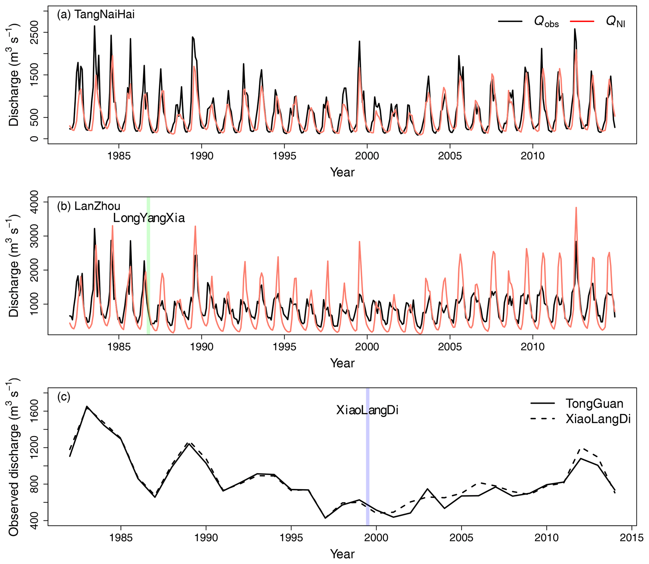
https://hess.copernicus.org/articles/25/1133/2021/hess-25-1133-2021-f04

Figure 4(a–b) Monthly observed (Q_obs) and simulated (Q_NI) streamflows at TangNaiHai and LanZhou stations. Green bar in (b) indicates the start of the LongYangXia dam regulation. (c) Observed annual streamflows at TongGuan and XiaoLangDi gauging stations, which are located up- and downstream of the XiaoLangDi reservoir, respectively (see Fig. 1). Blue bar in (c) indicates the start of the XiaoLangDi dam regulation.

Download

Regarding dams, before the operation of the LongYangXia dam in 1986, which brought a regulation capacity of 193.5×10⁸ m³ (green bar in Fig. 4b), the peaks of monthly Q_NI at LanZhou were slightly lower than the peaks of Q_obs in R₂ (Fig. 4b), as well as at TangNaiHai (Fig. 4a). But after the construction of the LongYangXia dam, modeled peak Q_NI became systematically higher than the peak of Q_obs each year, suggesting that the construction of this dam caused the observed peak reduction (Fig. 4b). Moreover, the seasonality of Q_obs changed dramatically in the period (1982–2014), but no similar trend was found in monthly P (Fig. S3), suggesting that dam operation was the primary driver of the observed shift in seasonal streamflow variations of the YRB from 1982 to 2014. Dams can affect inter-annual variations of Q as well, although less than the seasonal variation. For instance, TongGuan and XiaoLangDi are two consecutive gauging stations upstream and downstream of the reservoir of XiaoLangDi in R₄ (Fig. 1). The annual Q_obs at the two stations shows different features after the construction of the XiaoLangDi reservoir in 1999.

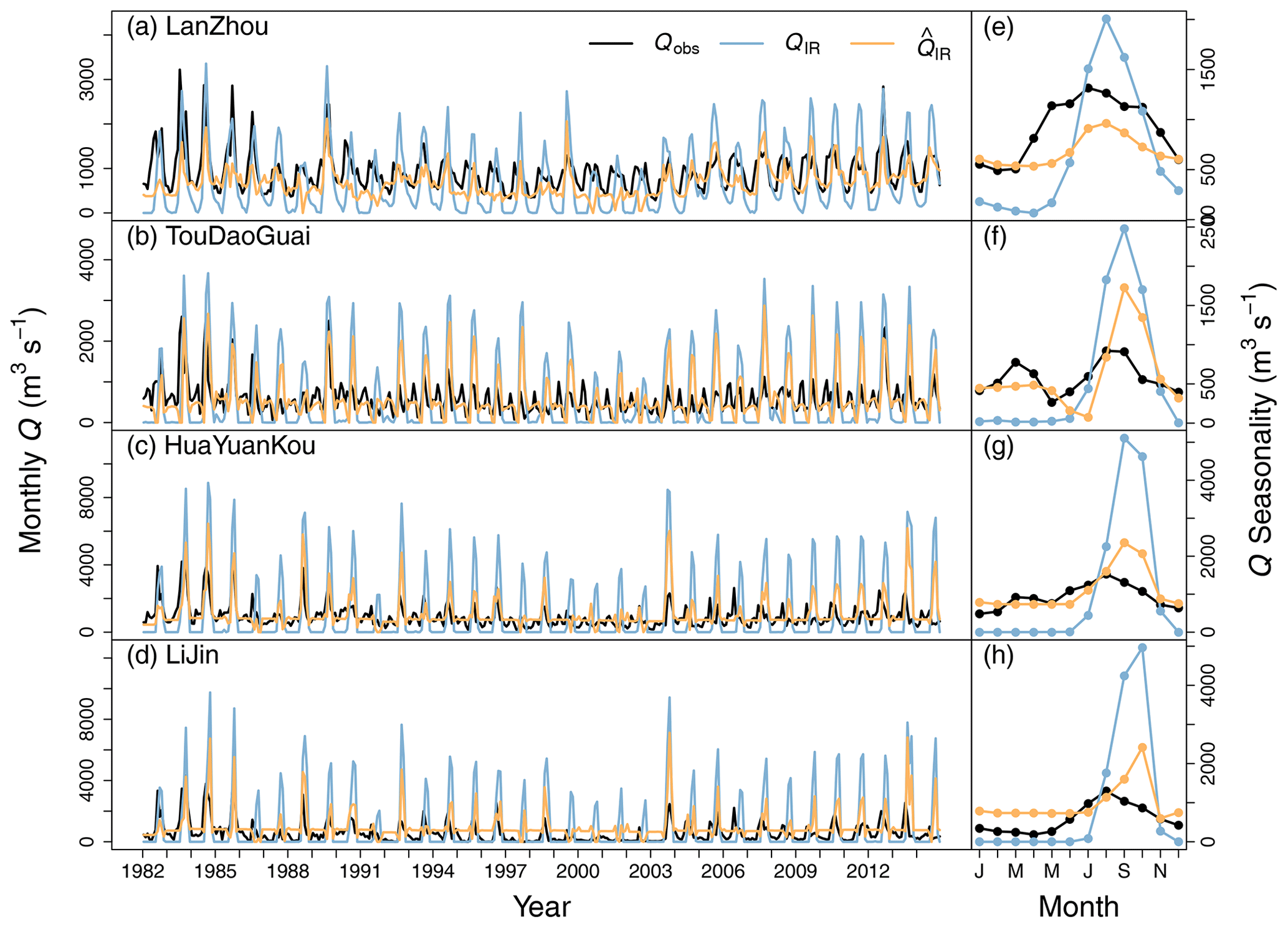
https://hess.copernicus.org/articles/25/1133/2021/hess-25-1133-2021-f05

Figure 5Comparison between observed and simulated actual monthly streamflows at gauging stations. Q_obs (dark lines) is observed monthly streamflows. Q_IR (blue lines) is simulated monthly streamflows from the IR experiment (Sect. 2.4). ${\hat{Q}}_{IR}$ (orange lines) is simulated monthly streamflows including impacts of dam regulation (Sect. 2.4).

Download

Figure 5 shows monthly time series of Q_obs, Q_IR, and ${\hat{Q}}_{IR}$ (see Sect. 2.1.2) at each gauging station. Discharge fluctuations are successfully improved in ${\hat{Q}}_{IR}$ . Especially the base flow of ${\hat{Q}}_{IR}$ coincides well with that of Q_obs during winter and spring. The only exception occurs at LiJin, where ${\hat{Q}}_{IR}$ overestimates the streamflows from January to May. In fact, the water release from XLD during this period would be withdrawn for irrigation and industry in R₅. However, our offline dam model is not able to simulate the interactions, leading to the overestimation.

The dam model is successful in reproducing flood control as well. At LanZhou, although ${\hat{Q}}_{IR}$ underestimates the peak flow due to the bias of the simulated mean annual streamflows (Fig. 3b), its seasonality is much smoother than that of Q_IR. The underestimation of ${\hat{Q}}_{IR}$ can reflect special water management during extreme years. From 2000 to 2002, the YRB experienced severe droughts, with 10 %–15 % precipitation less than usual, leading to a decrease of surface water resources by as much as 45 % (Water Resources Bulletin of China; http://www.mwr.gov.cn/sj/tjgb/szygb/, last access: 28 February 2021). To guarantee base flow, a set of policies were applied (e.g., reducing water withdrawn, increasing water price, and releasing more water from reservoirs). These policies are not accounted for in the model, which will produce a higher irrigation demand during dry years and promote the underestimation of the Q_obs. From TouDaoGuai to LiJin, the floods from August to October are dramatically reduced by our dam model. Nevertheless, the peaks are still overestimated in ${\hat{Q}}_{IR}$ , which might be due to numerous non-modeled medium/small reservoirs that were ignored by our model; no fewer than 203 medium reservoirs were documented at the end of 2014 (YRCC, 2014). In our simulation, a 326.5 ×10⁸ m³ regulation capacity is considered, which only accounts for 45 % of the total storage capacity of 720 ×10⁸ m³ (Ran and Lu, 2012). Moreover, in the five irrigation districts (http://www.yrcc.gov.cn/hhyl/yhgq/, last access: 28 February 2021; Tang et al., 2008), special irrigation systems in the YRB could contribute to flood reduction. For instance, the Hetao Plateau is the traditional irrigation district and is equipped with a hydraulic system that can divert river water into a complex irrigation network (bounded by 106.5–109^∘ E and 40.5–41.5^∘ N, shown in Fig. 1), by adjusting water level differences during the flood season. This no-dam diversion system of the Hetao Plateau can take 50 ×10⁸ m³ as an extra regulation capacity per year, equivalent to 14 % of the annual streamflow in R₃.

Simulated ΔW in R₂ is compared to observations (Jin et al., 2017) in the left panel of Fig. 6, and the good agreement suggests that our dam model is able to capture the seasonal variation of ΔW (r=0.9, p<0.001) and rectify the simulated streamflows. In the case of XiaoLangDi in the right panel of Fig. 6, where the correlation is smaller (r=0.34, p=0.28), the mismatch could be explained by sediment regulation procedures of that dam, given that it releases a huge amount of water in June for reservoir cleaning and sediment flushing downstream (Baoligao et al., 2016; Kong et al., 2017; Zhuo et al., 2019), a process not represented in our simple dam model. Moreover, because we ignored the buffering effect of numerous medium reservoirs, the simulated water recharge during the flood season could be overestimated.

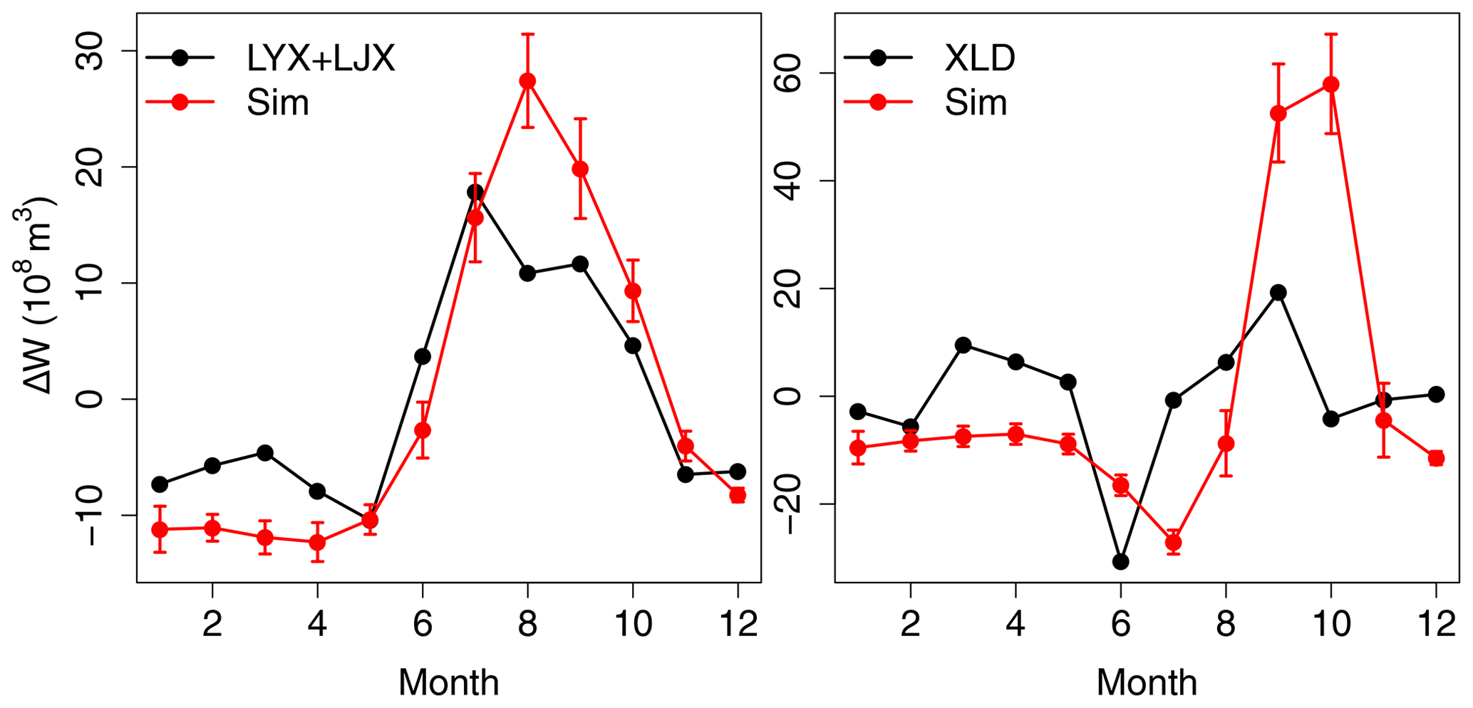
https://hess.copernicus.org/articles/25/1133/2021/hess-25-1133-2021-f06

Figure 6The changes of water storage of dams (ΔW) in R₂ and R₄. The dark line represents the ΔW from literature. The multi-year mean of ΔW of LongYangXia and LiuJiaXia is from Jin et al. (2017). The ΔW of XiaoLangDi is from the 1-year record reported in Kong et al. (2017). Red lines represent corresponding simulated ΔW from our dam regulation model.

Download

https://hess.copernicus.org/articles/25/1133/2021/hess-25-1133-2021-f07

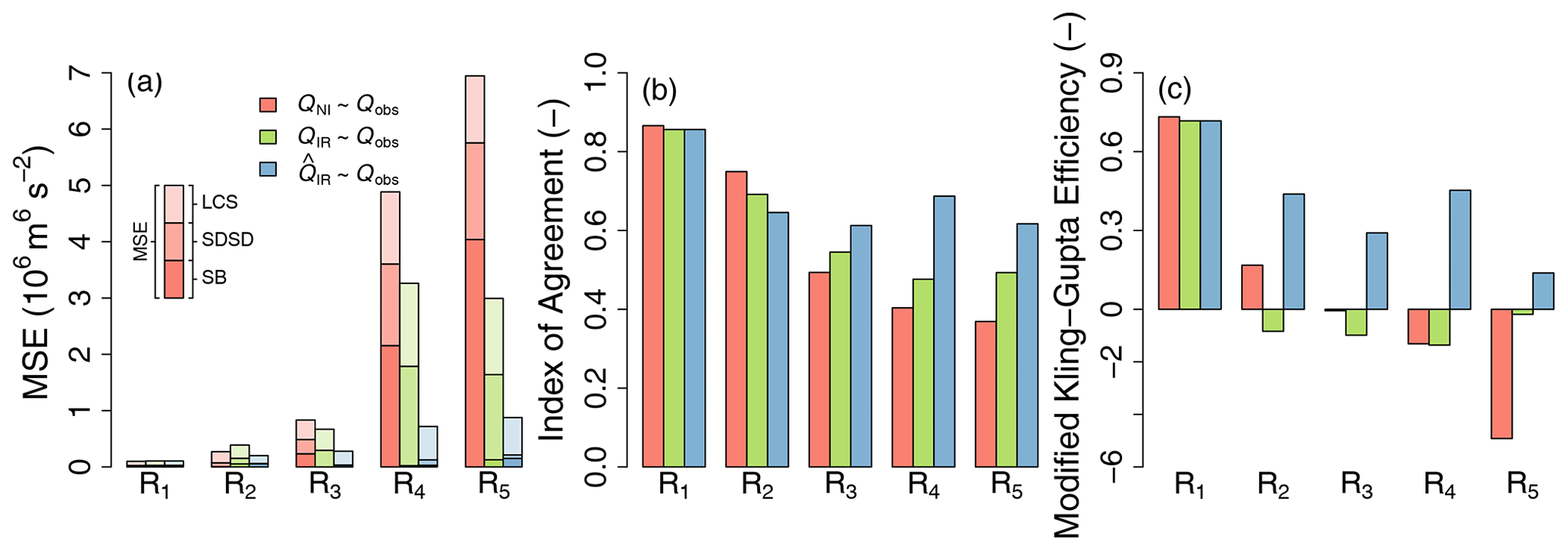
Figure 7Indicators of Q comparisons in each sub-catchment of the YRB. Colors indicate different comparisons. The MSE is decomposed to SB, SDSD, and LCS, which are distinguished by different transparencies.

Download

Figure 7 presents the model performances with different metrics in different R_i. The results show that MSE increases considerably from R₁ to R₅, implying accumulated impacts of error sources in increasing the error of modeled Q when going downstream in the entire catchment. Most likely, those error sources are omission errors of anthropogenic factors such as drinking and industrial water removals, but also of natural factors such as riparian wetlands and floodplains (e.g., the SanShengGong water conservancy hub) and non-represented small streams in the routing of ORCHIDEE (e.g., the irrigation system at the Hetao Plateau). From the decomposition of MSE, we found that adding irrigation to the model removes most of the bias in the average magnitude Q by reducing the SB bias error term of the MSE. The only exception occurs at LanZhou, where SB increases in IR, consequently leading to higher MSE. This misfit is due to the underestimation of Q upstream (Fig. 3a). Thus, modeled Q_IR is lower at LanZhou, which enlarges the SB. On the other hand, adding the dam operation contributes to improve the phase variations of Q which are dominated by the phase of the seasonal cycle, by reducing the SDSD error term. Nevertheless, the LCS error term, indicating the magnitude of the variability, mainly at inter-annual timescales, has no significant improvement with the representation of irrigation and dam regulations. It is because some of reservoirs are able to regulate Q inter-annually (Table 1), which can be observed from Fig. 4c. However, related operation rules are unclear and are not implemented in our dam model. Improvements were found in d as well, which demonstrates that the way human effects on Q of the YR were modeled brings more realistic results, despite ignoring the direct effect of irrigation demand on reservoir release and ignoring industrial and domestic water demands. The mKGE reveals a significant increase after considering dam operations (Fig. 7c). Particularly at LanZhou and HuaYuanKou, the mKGE of ${\hat{Q}}_{IR} \sim Q_{obs}$ increases by 0.86 and 1.11 compared to Q_IR∼Q_obs, respectively. Note that the mKGEs of Q_IR∼Q_obs are smaller than those of Q_NI∼Q_obs from R₂ to R₄ because irrigation decreases the mean annual streamflow of Q_IR, which further increases the CV_S, leading to worse γ in mKGE (Eq. 11).

4 Discussion

This study shows that ORCHIDEE land surface model with crops, irrigation, and our simple dam operation model can reproduce streamflow mean levels, inter-annual variations, and the seasonal cycle in different sub-catchments of the YRB correctly. We preliminarily quantified the impacts of irrigation and dams on the fluctuations of streamflows. Simulated water balance components were compared to observations in different sub-catchments with a good agreement (e.g., 4.5±6.9% for ET). We found that irrigation mainly affects the magnitude of annual streamflows by consuming $242.8 \pm 27.8 \times 10^{8}$ m³ yr⁻¹ of water, consistent with census data giving a consumption of $231.4 \pm 31.6 \times 10^{8}$ m³ yr⁻¹ (YRCC, 2014). As the water of the YRB is reaching the limit of usage (Feng et al., 2016), we did not find any significant effect of irrigation on streamflow trends. Instead of increasing river water withdrawals, the growing water demand appeared to have been balanced by improving water use efficiency during the study period (Yin et al., 2020; Zhou et al., 2020). Our simulation reveals that the impact of irrigation on streamflows may even be positive under special situations, which was also shown in Kustu et al. (2011). However, our mechanisms are different from the irrigation–ET–precipitation atmospheric feedback mechanisms found by Kustu et al. (2011); we demonstrated that irrigation may significantly increase soil moisture and promote runoff yield during the following wet season. It implies that irrigation in such landscapes may reinforce the magnitude of floods during the rainy season by a higher legacy soil moisture.

We found that dams strongly regulate the temporal variation of streamflows (Chen et al., 2016; Li et al., 2016; Yaghmaei et al., 2018). By including simple regulation rules depending on inflows, our dam model reduced the simulation error by 48 %–77 % (MSE in Fig. 7), especially the variability component (SDSD) of the total error, which is dominated by seasonal misfit reduction from dams. Moreover, we confirmed that the change of Q_obs seasonality during the study period is not due to climate change (Fig. S3) but is determined by dam operations (Wang et al., 2006). Big dams, like the LongYangXia, LiuJiaXia, and XiaoLangDi, are able to regulate streamflows inter-annually (Wang et al., 2018) and smooth the inter-annual distribution of water resources in the YRB (Piao et al., 2010; Wang et al., 2006; YRCC, 2014). However, their detailed operation rules are unclear and were not implemented explicitly in our dam model. The error corresponding to inter-annual variation (LCS in MSE in Fig. 7) was thus not reduced by including dams. In the dam model, some functions of reservoirs, such as providing irrigation supply, industrial and domestic water, electricity generation, and flood control (Basheer and Elagib, 2018), are not explicitly represented. Particularly the XiaoLangDi dam carries a distinctive water-sediment mission, which scours sediments downstream by creating artificial floods in June (Kong et al., 2017; Zhuo et al., 2019). These functions are associated with many socioeconomic factors and drivers, leading to competing demands for water (e.g., policies, electricity price, water price, land use change, irrigation techniques, water management techniques, and dams inter-connection), which are difficult to model well due to a lack of data. However, with the upcoming Surface Water and Ocean Topography (SWOT) mission, it will be possible to monitor the water level and surface extent of more reservoirs, which will be helpful to improve and validate the dam operation simulations (Ottlé et al., 2020).

Our simulations ignored potential impacts of reservoirs on local climate, e.g., through their evaporation (Degu et al., 2011). The water area of several artificial reservoirs (LongYangXia, LiuJiaXia, BoHaiWan, SanShengGong, and XiaoLangDi) is approximately 1056 km², which is larger than the 10th largest natural lake in China. These water bodies can also significantly influence local energy budgets, and evaporative water loss may be considerable, especially in arid and semi-arid areas (Friedrich et al., 2018; Shiklomanov, 1999). In addition, the five large irrigation districts (http://www.yrcc.gov.cn/hhyl/yhgq/, last access: 27 February 2021) could dramatically alter the local climate through atmospheric feedbacks. For instance, the Hetao Plateau can take about 50 ×10⁸ m³ from streamflows every year during the flood season. Its irrigation area is 5740 km², with an evapotranspiration rate ranging between 1200–1600 mm yr⁻¹. However, as these irrigation districts divert river water without big dams, they are not taken into account in most YR studies. Another non-negligible factor in the case of YR is sedimentation, which reduces the regulation capacities of reservoirs and weakens streamflow regulation by humans. For instance, the total capacity of QingTongXia has declined from 6.06 to 0.4×10⁸ m³ since 1978 due to sedimentation. Therefore, how land use change and the evolution of natural ecosystems affect sediment load and deposition is another key factor to project dams' disturbances on streamflows in the YRB.

Simulating anthropogenic impact on river streamflows is challenging. In the case of the YR, well-calibrated models can provide accurate naturalized streamflow simulations, with Nash–Sutcliffe efficiency (NSE) as high as 0.9 (Yuan et al., 2016). However, when considering the impacts of irrigation and dams, the NSE values of simulations are generally worse. For instance, simulations with anthropogenic effects by Hanasaki et al. (2018) had lower NSE than the simulation with only natural processes. Similarly, Wada et al. (2014) showed NSE decrease after considering anthropogenic factors in the YRB, which was interpreted as complexity of the YRB under the impacts of human activities and climate variation. However, the NSE of naturalized streamflows cannot really be compared to the one of regulated streamflows. Even if a model can perfectly simulate the dam operations, the NSE of naturalized streamflows will be larger than that of regulated streamflows, given that dam operations automatically reduce the variation of river streamflows (a simple proof is available in Sect. A of the Supplement). In fact, our model performances are very similar to GHM simulations (Fig. S2 from Liu et al., 2019). By gradually considering anthropogenic factors (irrigation and dam operations), the performances of our simulations increase dramatically according to all three metrics.

Intensive calibrations using a suite of observations can allow catchment-scale studies to provide highly accurate simulated streamflows for short-term flood forecasts. However, for long-term projections, a model should include all key processes of the system studied. If key processes are missing in the model, a calibration will cover up the shortcomings, which lead to a lack of predictive capacities for long timescales, as shown by Duethmann et al. (2020). Therefore, by developing crop physiology and phenology, irrigation, and a (offline) dam operation model, we have tried to demonstrate that streamflow fluctuations of the YR can be reasonably reproduced by a generic land surface model. Although mismatches exist in the simulated streamflows, they are more likely caused by missing processes (joint impact of multiple medium reservoirs, special mission of dams, irrigation system characteristics) than by poor calibration of existing processes because other simulated hydrological variables coincide well with observations in the YRB, such as soil moisture dynamics (Yin et al., 2018), naturalized river streamflows (Table S1 in Xi et al., 2018), leaf area index (Sect. S2 in Xi et al., 2018), amount and trend of irrigation withdrawals (Yin et al., 2020), trends of total water storage (Sect. 3.4 in Yin et al., 2020), and ET (Table S2). On the contrary, these mismatches draw our attention to some key mechanisms overlooked in most models. For instance, our model underestimates the annual streamflow at LanZhou in the period 2000–2002 (Fig. 3b), during which ${\hat{Q}}_{IR}$ was almost negatively correlated to the Q_obs (Fig. 5a). In summary, our results show that the errors of simulated streamflows decreased dramatically after considering crops, irrigation, and dam operations, suggesting that these are first-order mechanisms controlling streamflow fluctuations. Future work can be focused on completing the model by linking dam operation to the variable crop water demand.

5 Conclusions

A land surface model ORCHIDEE and a newly developed dam model are utilized to simulate the streamflow fluctuations and dam operations in the Yellow River basin. The impacts of irrigation and dam regulation on streamflow fluctuations of the Yellow River were preliminarily qualified and quantified in this study by using a process-based land surface model and a dam operation model. Irrigation mainly contributes to the reduction of annual streamflow by as much as $242.8 \pm 27.8 \times 10^{8}$ m³ yr⁻¹. The shifts of intra-annual variation of the Yellow River streamflows appear not to be caused by climate change, at least not by significant changes of precipitation patterns and land use during the study period, but by the construction of dams and their operation. After considering the impacts of dams, we found that dam regulation can explain about 48 %–77 % of the fluctuations of streamflows. The effect of dams may be still underestimated because we only considered simple regulation rules based on inflows but ignored its interactions with irrigation demand downstream. Moreover, our analysis showed that several reservoirs on the Yellow River are able to influence streamflows inter-annually. However, such effects are not quantified due to a lack of knowledge of the regulation rules across our study period.

Code and data availability

The code of ORCHIDEE can be assessed via https://forge.ipsl.jussieu.fr/orchidee/browser/branches/ORCHIDEE-MICT (Yin et al., 2020). The data used in this study, and the code of the dam operation model, analysis, and plotting can be accessed via https://doi.org/10.5281/zenodo.3979053 (Yin, 2020). The GLEAM ET data can be downloaded from http://gleam.eu (Global Land Evaporation Amsterdam Model, 2021; Martens et al., 2017). The MSWEP precipitation data and the PKU ET are available from http://gloh2o.org (GLOH2O, 2021; Beck et al., 2017) and Zhenzhong Zeng (Zeng et al., 2014), respectively, and can be obtained upon reasonable request.

Supplement

The supplement related to this article is available online at: https://doi.org/10.5194/hess-25-1133-2021-supplement.

Author contributions

ZY, CO, and PC designed this study; ZY and XW contributed to the model development; ZY, FZ, XW, XZ, YB, and YX prepared observation datasets; ZY performed model simulations and primary analysis and drafted the manuscript; all authors contributed to results interpretation, additional analysis, and manuscript revisions.

Competing interests

The authors declare that they have no conflict of interest.

Acknowledgements

We would like to thank the editor and the two anonymous referees for their insightful comments and efforts. We gratefully acknowledge the GLEAM team, the FLUXCOM team, Hyungjun Kim, Hylke Beck, and Zenzhong Zeng for their selfless sharing of their datasets.

Financial support

This research has been supported by the Agence Nationale de la Recherche (grant no. ANR-15-CE01-00L1-0L), the National Natural Science Foundation of China (grant no. 41561134016), and the French Space Agency (Centre National d'Etudes Spatiales) through the TOSCA-SPAWET program in preparation for the international SWOT space mission. Feng Zhou was supported by the National Key Research and Development Program of China (grant no. 2016YFD0800501).

Review statement

This paper was edited by Xing Yuan and reviewed by two anonymous referees.

References

Baoligao, B. Y., Xu, F. R., Chen, X. R., Wang, X. Y., and Chen, W. X.: Acute impacts of reservoir sediment flushing on fishes in the Yellow River, J. Hydrol.-Environ. Res., 13, 26–35, https://doi.org/10.1016/j.jher.2015.11.003, 2016. a

Basheer, M. and Elagib, N. A.: Sensitivity of Water-Energy Nexus to dam operation: A Water-Energy Productivity concept, Sci. Total Environ., 617, 918–926, https://doi.org/10.1016/j.scitotenv.2017.10.228, 2018. a

Beck, H. E., van Dijk, A. I. J. M., Levizzani, V., Schellekens, J., Miralles, D. G., Martens, B., and de Roo, A.: MSWEP: 3-hourly 0.25° global gridded precipitation (1979–2015) by merging gauge, satellite, and reanalysis data, Hydrol. Earth Syst. Sci., 21, 589–615, https://doi.org/10.5194/hess-21-589-2017, 2017. a, b

Becker, A., Finger, P., Meyer-Christoffer, A., Rudolf, B., Schamm, K., Schneider, U., and Ziese, M.: A description of the global land-surface precipitation data products of the Global Precipitation Climatology Centre with sample applications including centennial (trend) analysis from 1901–present, Earth Syst. Sci. Data, 5, 71–99, https://doi.org/10.5194/essd-5-71-2013, 2013. a

Biemans, H., Haddeland, I., Kabat, P., Ludwig, F., Hutjes, R. W. A., Heinke, J., Von Bloh, W., and Gerten, D.: Impact of reservoirs on river discharge and irrigation water supply during the 20th century, Water Resour. Res., 47, W03509, https://doi.org/10.1029/2009WR008929, 2011. a, b

Bondeau, A., Smith, P. C., Zaehle, S., Schaphoff, S., Lucht, W., Cramer, W., Gerten, D., Lotze-Campen, H., Müller, C., Reichstein, M., and Smith, B.: Modelling the role of agriculture for the 20th century global terrestrial carbon balance, Glob. Change Biol., 13, 679–706, https://doi.org/10.1111/j.1365-2486.2006.01305.x, 2007. a

Bureau of Reclamation: Colorado River Basin Water Supply and Demand Study, Technical Report, Department of the Interior Bureau of Reclamation, Phoenix, USA, available at: http://www.riversimulator.org/Resources/USBR/BasinStudy/BasinStudyDocumentsCombined.pdf (last access: 28 February 2021), 2012. a

Chen, J., Finlayson, B. L., Wei, T. Y., Sun, Q. L., Webber, M., Li, M. T., and Chen, Z. Y.: Changes in monthly flows in the Yangtze River, China – With special reference to the Three Gorges Dam, J. Hydrol., 536, 293–301, https://doi.org/10.1016/j.jhydrol.2016.03.008, 2016. a

Chen, Y. Y., Yang, K., He, J., Qin, J., Shi, J. C., Du, J. Y., and He, Q.: Improving land surface temperature modeling for dry land of China, J. Geophys. Res., 116, D20104, https://doi.org/10.1029/2011JD015921, 2011. a

Degu, A. M., Hossain, F., Niyogi, D., Pielke, R., Shepherd, J. M., Voisin, N., and Chronis, T.: The influence of large dams on surrounding climate and precipitation patterns, Geophys. Res. Lett., 38, L04405, https://doi.org/10.1029/2010GL046482, 2011. a

Deryng, D., Sacks, W. J., Barford, C. C., and Ramankutty, N.: Simulating the effects of climate and agricultural management practices on global crop yield, Global Biogeochem. Cy., 25, GB2006, https://doi.org/10.1029/2009gb003765, 2011. a

Deryng, D., Conway, D., Ramankutty, N., Price, J., and Warren, R.: Global crop yield response to extreme heat stress under multiple climate change futures, Environ. Res. Lett., 9, 034011, https://doi.org/10.1088/1748-9326/9/3/034011, 2014. a

de Wit, A. J. W. and van Diepen, C. A.: Crop growth modelling and crop yield forecasting using satellite-derived meteorological inputs, Int. J. Appl. Earth Obs., 10, 414–425, https://doi.org/10.1016/j.jag.2007.10.004, 2008. a

Drewniak, B., Song, J., Prell, J., Kotamarthi, V. R., and Jacob, R.: Modeling agriculture in the Community Land Model, Geosci. Model Dev., 6, 495–515, https://doi.org/10.5194/gmd-6-495-2013, 2013. a

Droppers, B., Franssen, W. H. P., van Vliet, M. T. H., Nijssen, B., and Ludwig, F.: Simulating human impacts on global water resources using VIC-5, Geosci. Model Dev., 13, 5029–5052, https://doi.org/10.5194/gmd-13-5029-2020, 2020. a

Duethmann, D., Blöschl, G., and Parajka, J.: Why does a conceptual hydrological model fail to correctly predict discharge changes in response to climate change?, Hydrol. Earth Syst. Sci., 24, 3493–3511, https://doi.org/10.5194/hess-24-3493-2020, 2020. a, b

Elliott, J., Kelly, D., Chryssanthacopoulos, J., Glotter, M., Jhunjhnuwala, K., Best, N., Wilde, M., and Foster, I.: The parallel system for integrating impact models and sectors (pSIMS), Environ. Modell. Softw., 62, 509–516, https://doi.org/10.1016/j.envsoft.2014.04.008, 2014. a

Feng, X. M., Fu, B. J., Piao, S. L., Wang, S., Ciais, P., Zeng, Z. Z., Lü, Y. H., Zeng, Y., Li, Y., Jiang, X. H., and Wu, B. F.: Revegetation in China's Loess Plateau is approaching sustainable water resource limits, Nat. Clim. Change, 6, 1019–1022, https://doi.org/10.1038/nclimate3092, 2016. a

Folberth, C., Gaiser, T., Abbaspour, K. C., Schulin, R., and Yang, H.: Regionalization of a large-scale crop growth model for sub-Saharan Africa: Model setup, evaluation, and estimation of maize yields, Agr. Ecosyst. Environ., 151, 21–33, https://doi.org/10.1016/j.agee.2012.01.026, 2012. a

Friedrich, K., Grossman, R. L., Huntington, J., Blanken, P. D., Lenters, J., Holman, K. D., Gochis, D., Livneh, B., Prairie, J., Skeie, E., Healey, N. C., Dahm, K., Pearson, C., Finnessey, T., Hook, S. J., and Kowalski, T.: Reservoir Evaporation in the Western United States: Current Science, Challenges, and Future Needs, B. Am. Meteorol. Soc., 99, 167–187, https://doi.org/10.1175/BAMS-D-15-00224.1, 2018. a

Global Land Evaporation Amsterdam Model (GLEAM), available at: http://gleam.eu, last access: 1 March 2021. a

GLOH2O: Multi-Source Weighted-Ensemble Precipitation (MSWEP from GLOH2O), available at: http://gloh2o.org, last access: 1 March 2021. a

Grill, G., Lehner, B., Thieme, M., Geenen, B., Tickner, D., Antonelli, F., Babu, S., Borrelli, P., Cheng, L., Crochetiere, H., Ehalt Macedo, H., Filgueiras, R., Goichot, M., Higgins, J., Hogan, Z., Lip, B., McClain, M. E., Meng, J., Mulligan, M., Nilsson, C., Olden, J. D., Opperman, J. J., Petry, P., Reidy Liermann, C., Sáenz, L., Salinas-Rodríguez, S., Schelle, P., Schmitt, R. J. P., Snider, J., Tan, F., Tockner, K., Valdujo, P. H., van Soesbergen, A., and Zarfl, C.: Mapping the world's free-flowing rivers, Nature, 569, 215–221, https://doi.org/10.1038/s41586-019-1111-9, 2019. a

Gupta, H. V., Kling, H., Yilmaz, K. K., and Martinez, G. F.: Decomposition of the mean squared error and NSE performance criteria: Implications for improving hydrological modelling, J. Hydrol., 377, 80–91, https://doi.org/10.1016/j.jhydrol.2009.08.003, 2009. a

Haddeland, I., Lettenmaier, D. P., and Skaugen, T.: Effects of irrigation on the water and energy balances of the Colorado and Mekong river basins, J. Hydrol., 324, 210–223, https://doi.org/10.1016/j.jhydrol.2005.09.028, 2006. a

Haddeland, I., Heinke, J., Biemans, H., Eisner, S., Flörke, M., Hanasaki, N., Konzmann, M., Ludwig, F., Masaki, Y., Schewe, J., Stacke, T., Tessler, Z. D., Wada, Y., and Wisser, D.: Global water resources affected by human interventions and climate change, P. Natl. Acad. Sci. USA, 111, 3251–3256, https://doi.org/10.1073/pnas.1222475110, 2014. a, b

Hanasaki, N., Kanae, S., and Oki, T.: A reservoir operation scheme for global river routing models, J. Hydrol., 327, 22–41, https://doi.org/10.1016/j.jhydrol.2005.11.011, 2006. a, b, c, d, e, f

Hanasaki, N., Kanae, S., Oki, T., Masuda, K., Motoya, K., Shirakawa, N., Shen, Y., and Tanaka, K.: An integrated model for the assessment of global water resources – Part 1: Model description and input meteorological forcing, Hydrol. Earth Syst. Sci., 12, 1007–1025, https://doi.org/10.5194/hess-12-1007-2008, 2008. a

Hanasaki, N., Fujimori, S., Yamamoto, T., Yoshikawa, S., Masaki, Y., Hijioka, Y., Kainuma, M., Kanamori, Y., Masui, T., Takahashi, K., and Kanae, S.: A global water scarcity assessment under Shared Socio-economic Pathways – Part 2: Water availability and scarcity, Hydrol. Earth Syst. Sci., 17, 2393–2413, https://doi.org/10.5194/hess-17-2393-2013, 2013. a

Hanasaki, N., Yoshikawa, S., Pokhrel, Y., and Kanae, S.: A global hydrological simulation to specify the sources of water used by humans, Hydrol. Earth Syst. Sci., 22, 789–817, https://doi.org/10.5194/hess-22-789-2018, 2018. a, b, c, d, e

Humphries, P., Keckeis, H., and Finlayson, B.: The River Wave Concept: Integrating River Ecosystem Models, BioScience, 64, 870–882, https://doi.org/10.1093/biosci/biu130, 2014. a

IPCC: Climate Change 2014: Synthesis Report. Contribution of Working Groups I, II and III to the Fifth Assessment Report of the Intergovernmental Panel on Climate Change, edited by: Pachauri, R. K. and Meyer, L. A., IPCC, Geneva, Switzerland, 151 pp., 2014. a

Izaurralde, R. C., Williams, J. R., McGill, W. B., Rosenberg, N. J., and Jakas, M. Q.: Simulating soil C dynamics with EPIC: Model description and testing against long-term data, Ecol. Model., 192, 362–384, https://doi.org/10.1016/j.ecolmodel.2005.07.010, 2006. a

Jia, Y. W., Wang, H., Zhou, Z. H., Qiu, Y. Q., Luo, X. Y., Wang, J. H., Yan, D. H., and Qin, D. Y.: Development of the WEP-L distributed hydrological model and dynamic assessment of water resources in the Yellow River basin, J. Hydrol., 331, 606–629, https://doi.org/10.1016/j.jhydrol.2006.06.006, 2006. a, b

Jin, S. Y., Zhang, P., and Zhao, W. R.: Analysis of flow process variation degree and influencing factors in inner Mongolia reach of the Yellow River, IOP Conference Series: Earth and Environmental Science, 69, 012015, https://doi.org/10.1088/1755-1315/69/1/012015, 2017. a, b, c

Jones, J. W., Hoogenboom, G., Porter, C. H., Boote, K. J., Batchelor, W. D., Hunt, L. A., Wilkens, P. W., Singh, U., Gijsman, A. J., and Ritchie, J. T.: The DSSAT cropping system model, Eur. J. Agron., 18, 235–265, https://doi.org/10.1016/S1161-0301(02)00107-7, 2003. a

Jung, M., Reichstein, M., and Bondeau, A.: Towards global empirical upscaling of FLUXNET eddy covariance observations: validation of a model tree ensemble approach using a biosphere model, Biogeosciences, 6, 2001–2013, https://doi.org/10.5194/bg-6-2001-2009, 2009. a

Keating, B. A., Carberry, P. S., Hammer, G. L., Probert, M. E., Robertson, M. J., Holzworth, D., Huth, N. I., Hargreaves, J. N., Meinke, H., Hochman, Z., McLean, G., Verburg, K., Snow, V., Dimes, J. P., Silburn, M., Wang, E., Brown, S., Bristow, K. L., Asseng, S., Chapman, S., McCown, R. L., Freebairn, D. M., and Smith, C. J.: An overview of APSIM, a model designed for farming systems simulation, Eur. J. Agron., 18, 267–288, https://doi.org/10.1016/S1161-0301(02)00108-9, 2003. a

Kim, H.: Global Soil Wetness Project Phase 3 Atmospheric Boundary Conditions, Experiment 1, DIAS, https://doi.org/10.20783/DIAS.501, 2017. a

Kling, H., Fuchs, M., and Paulin, M.: Runoff conditions in the upper Danube basin under an ensemble of climate change scenarios, J. Hydrol., 424/425, 264–277, https://doi.org/10.1016/j.jhydrol.2012.01.011, 2012. a

Kobayashi, K. and Salam, M. U.: Comparing Simulated and Measured Values Using Mean Squared Deviation and its Components, Agron. J., 92, 345, https://doi.org/10.1007/s100870050043, 2000. a, b

Kong, D. X., Miao, C. Y., Wu, J. W., Borthwick, A. G. L., Duan, Q. Y., and Zhang, X. M.: Environmental impact assessments of the Xiaolangdi Reservoir on the most hyperconcentrated laden river, Yellow River, China, Environ. Sci. Pollut. R., 24, 4337–4351, https://doi.org/10.1007/s11356-016-7975-4, 2017. a, b, c

Kustu, M. D., Fan, Y., and Rodell, M.: Possible link between irrigation in the US High Plains and increased summer streamflow in the Midwest, Water Resour. Res., 47, W03522, https://doi.org/10.1029/2010WR010046, 2011. a, b

Leng, G. Y., Tang, Q. H., Huang, M. Y., and Leung, L. R.: A comparative analysis of the impacts of climate change and irrigation on land surface and subsurface hydrology in the North China Plain, Reg. Environ. Change, 15, 251–263, https://doi.org/10.1007/s10113-014-0640-x, 2015. a

Li, C., Yang, S. Y., Lian, E. G., Yang, C. F., Deng, K., and Liu, Z. F.: Damming effect on the Changjiang (Yangtze River) river water cycle based on stable hydrogen and oxygen isotopic records, J. Geochem. Explor., 165, 125–133, https://doi.org/10.1016/j.gexplo.2016.03.006, 2016. a

Lindeskog, M., Arneth, A., Bondeau, A., Waha, K., Seaquist, J., Olin, S., and Smith, B.: Implications of accounting for land use in simulations of ecosystem carbon cycling in Africa, Earth Syst. Dynam., 4, 385–407, https://doi.org/10.5194/esd-4-385-2013, 2013. a

Liu, C. M. and Zhang, S. F.: Drying up of the yellow river: its impacts and counter-measures, Mitig. Adapt. Strat. Gl., 7, 203–214, https://doi.org/10.1023/A:1024408310869, 2002. a

Liu, H., Jia, Y. W., Niu, C. W., Su, H. D., Wang, J. H., Du, J. K., Khaki, M., Hu, P., and Liu, J. J.: Development and validation of a physically-based, national-scale hydrological model in China, J. Hydrol., 590, 125431, https://doi.org/10.1016/j.jhydrol.2020.125431, 2020. a

Liu, J. G., Wiberg, D., Zehnder, A. J. B., and Yang, H.: Modeling the role of irrigation in winter wheat yield, crop water productivity, and production in China, Irrigation Sci., 26, 21–33, https://doi.org/10.1007/s00271-007-0069-9, 2007. a

Liu, J. G., Zhao, D. D., Gerbens-Leenes, P. W., and Guan, D. B.: China's rising hydropower demand challenges water sector, Sci. Rep., 5, 11446, https://doi.org/10.1038/srep11446, 2015. a

Liu, J. G., Yang, H., Gosling, S. N., Kummu, M., Flörke, M., Pfister, S., Hanasaki, N., Wada, Y., Zhang, X. X., Zheng, C. M., Alcamo, J., and Oki, T.: Water scarcity assessments in the past, present, and future, Earths Future, 5, 545–559, https://doi.org/10.1002/2016EF000518, 2017. a

Liu, W. F., Yang, H., Folberth, C., Wang, X. Y., Luo, Q. Y., and Schulin, R.: Global investigation of impacts of PET methods on simulating crop-water relations for maize, Agr. Forest Meteorol., 221, 164–175, https://doi.org/10.1016/j.agrformet.2016.02.017, 2016. a

Liu, X., Liu, W., Yang, H., Tang, Q., Flörke, M., Masaki, Y., Müller Schmied, H., Ostberg, S., Pokhrel, Y., Satoh, Y., and Wada, Y.: Multimodel assessments of human and climate impacts on mean annual streamflow in China, Hydrol. Earth Syst. Sci., 23, 1245–1261, https://doi.org/10.5194/hess-23-1245-2019, 2019. a, b

Lohmann, D., Raschke, E., Nijssen, B., and Lettenmaier, D. P.: Hydrologie à l'échelle régionale: I. Formulation du modèle VIC-2L couplé à un modèle du transfert de l'eau, Hydrolog. Sci. J., 43, 131–141, https://doi.org/10.1080/02626669809492107, 1998. a

Martens, B., Miralles, D. G., Lievens, H., van der Schalie, R., de Jeu, R. A. M., Fernández-Prieto, D., Beck, H. E., Dorigo, W. A., and Verhoest, N. E. C.: GLEAM v3: satellite-based land evaporation and root-zone soil moisture, Geosci. Model Dev., 10, 1903–1925, https://doi.org/10.5194/gmd-10-1903-2017, 2017. a, b

Miao, C. Y., Ni, J. R., Borthwick, A. G. L., and Yang, L.: A preliminary estimate of human and natural contributions to the changes in water discharge and sediment load in the Yellow River, Global Planet. Change, 76, 196–205, https://doi.org/10.1016/j.gloplacha.2011.01.008, 2011. a

Müller, C., Elliott, J., Chryssanthacopoulos, J., Arneth, A., Balkovic, J., Ciais, P., Deryng, D., Folberth, C., Glotter, M., Hoek, S., Iizumi, T., Izaurralde, R. C., Jones, C., Khabarov, N., Lawrence, P., Liu, W., Olin, S., Pugh, T. A. M., Ray, D. K., Reddy, A., Rosenzweig, C., Ruane, A. C., Sakurai, G., Schmid, E., Skalsky, R., Song, C. X., Wang, X., de Wit, A., and Yang, H.: Global gridded crop model evaluation: benchmarking, skills, deficiencies and implications, Geosci. Model Dev., 10, 1403–1422, https://doi.org/10.5194/gmd-10-1403-2017, 2017. a

Nazemi, A. and Wheater, H. S.: On inclusion of water resource management in Earth system models – Part 1: Problem definition and representation of water demand, Hydrol. Earth Syst. Sci., 19, 33–61, https://doi.org/10.5194/hess-19-33-2015, 2015. a

Ngo-Duc, T., Laval, K., Ramillien, G., Polcher, J., and Cazenave, A.: Validation of the land water storage simulated by Organising Carbon and Hydrology in Dynamic Ecosystems (ORCHIDEE) with Gravity Recovery and Climate Experiment (GRACE) data, Water Resour. Res., 43, 1–8, https://doi.org/10.1029/2006WR004941, 2007. a

Ottlé, C., Bernus, A., Verbeke, T., Pétrus, K., Yin, Z., Biancamaria, S., Jost, A., Desroches, D., Pottier, C., Perrin, C., de Lavenne, A., Flipo, N., and Rivière, A.: Characterization of SWOT Water Level Errors on Seine Reservoirs and La Bassée Gravel Pits: Impacts on Water Surface Energy Budget Modeling, Remote Sens., 12, 2911, https://doi.org/10.3390/rs12182911, 2020. a

Piao, S., Friedlingstein, P., Ciais, P., de Noblet-Ducoudre, N., Labat, D., and Zaehle, S.: Changes in climate and land use have a larger direct impact than rising CO₂ on global river runoff trends, P. Natl. Acad. Sci. USA, 104, 15242–15247, https://doi.org/10.1073/pnas.0707213104, 2007. a

Piao, S. L., Ciais, P., Huang, Y., Shen, Z. H., Peng, S. S., Li, J. S., Zhou, L. P., Liu, H. Y., Ma, Y. C., Ding, Y. H., Friedlingstein, P., Liu, C. Z., Tan, K., Yu, Y. Q., Zhang, T. Y., and Fang, J. Y.: The impacts of climate change on water resources and agriculture in China, Nature, 467, 43–51, https://doi.org/10.1038/nature09364, 2010. a, b, c

Ran, L. S. and Lu, X. X.: Delineation of reservoirs using remote sensing and their storage estimate: An example of the Yellow River basin, China, Hydrol. Process., 26, 1215–1229, https://doi.org/10.1002/hyp.8224, 2012. a

Seneviratne, S. I., Donat, M. G., Mueller, B., and Alexander, L. V.: No pause in the increase of hot temperature extremes, Nat. Clim. Change, 4, 161–163, https://doi.org/10.1038/nclimate2145, 2014. a

Sherwood, S. and Fu, Q.: A Drier Future?, Science, 343, 737–739, https://doi.org/10.1126/science.1247620, 2014. a

Shiklomanov, I. A.: State Hydrological Institute (SHL. St. Petersburg) and United Nations Educational, Scientific and Cultural Organisation, UNESCO, Paris, 1999. a

Smith, B., Prentice, I. C., and Sykes, M. T.: Representation of vegetation dynamics in the modelling of terrestrial ecosystems: comparing two contrasting approaches within European climate space, Global Ecol. Biogeogr., 10, 621–637, https://doi.org/10.1046/j.1466-822X.2001.00256.x, 2001. a

Tang, Q. H., Oki, T., Kanae, S., and Hu, H. P.: Hydrological Cycles Change in the Yellow River Basin during the Last Half of the Twentieth Century, J. Climate, 21, 1790–1806, https://doi.org/10.1175/2007JCLI1854.1, 2008. a, b, c, d

Thiery, W., Davin, E. L., Lawrence, D. M., Hirsch, A. L., Hauser, M., and Seneviratne, S. I.: Present-day irrigation mitigates heat extremes, J. Geophys. Res.-Atmos., 122, 1403–1422, https://doi.org/10.1002/2016JD025740, 2017. a

Voisin, N., Li, H., Ward, D., Huang, M., Wigmosta, M., and Leung, L. R.: On an improved sub-regional water resources management representation for integration into earth system models, Hydrol. Earth Syst. Sci., 17, 3605–3622, https://doi.org/10.5194/hess-17-3605-2013, 2013. a, b

Wada, Y., Wisser, D., and Bierkens, M. F. P.: Global modeling of withdrawal, allocation and consumptive use of surface water and groundwater resources, Earth Syst. Dynam., 5, 15–40, https://doi.org/10.5194/esd-5-15-2014, 2014. a, b, c, d, e

Wada, Y., de Graaf, I. E. M., and van Beek, L. P. H.: High-resolution modeling of human and climate impacts on global water resources, J. Adv. Model. Earth Sy., 8, 735–763, https://doi.org/10.1002/2015MS000618, 2016. a, b, c

Waha, K., Van Bussel, L. G. J., Müller, C., and Bondeau, A.: Climate-driven simulation of global crop sowing dates, Global Ecol. Biogeogr., 21, 247–259, https://doi.org/10.1111/j.1466-8238.2011.00678.x, 2012. a

Wang, H. J., Yang, Z. S., Saito, Y., Liu, J. P., and Sun, X. X.: Interannual and seasonal variation of the Huanghe (Yellow River) water discharge over the past 50 years: Connections to impacts from ENSO events and dams, Global Planet. Change, 50, 212–225, https://doi.org/10.1016/j.gloplacha.2006.01.005, 2006. a, b, c, d

Wang, S. S., Mo, X. G., Liu, S. X., Lin, Z. H., and Hu, S.: Validation and trend analysis of ECV soil moisture data on cropland in North China Plain during 1981–2010, Int. J. Appl. Earth Obs., 48, 110–121, https://doi.org/10.1016/j.jag.2015.10.010, 2016. a

Wang, X. H.: Impacts of environmental change on rice ecosystems in China: development, optimization and application of ORCHIDEE-CROP model, PhD thesis, Peking University, Peking, China, 174 pp., 2016. a, b, c, d

Wang, X. H., Ciais, P., Li, L., Ruget, F., Vuichard, N., Viovy, N., Zhou, F., Chang, J. F., Wu, X. C., Zhao, H. F., and Piao, S. L.: Management outweighs climate change on affecting length of rice growing period for early rice and single rice in China during 1991–2012, Agr. Forest Meteorol., 233, 1–11, https://doi.org/10.1016/j.agrformet.2016.10.016, 2017. a, b, c, d, e

Wang, X. J., Engel, B., Yuan, X. M., and Yuan, P. X.: Variation Analysis of Streamflows from 1956 to 2016 Along the Yellow River, China, Water, 10, 1231, https://doi.org/10.3390/w10091231, 2018. a, b

Williams, J. R.: The EPIC Model, in: Computer Models of Watershed Hydrology, edited by: Singh, V. P., Water Resources Publications, Colorado, USA, 909–1000, 1995. a

Wu, X., Vuichard, N., Ciais, P., Viovy, N., de Noblet-Ducoudré, N., Wang, X., Magliulo, V., Wattenbach, M., Vitale, L., Di Tommasi, P., Moors, E. J., Jans, W., Elbers, J., Ceschia, E., Tallec, T., Bernhofer, C., Grünwald, T., Moureaux, C., Manise, T., Ligne, A., Cellier, P., Loubet, B., Larmanou, E., and Ripoche, D.: ORCHIDEE-CROP (v0), a new process-based agro-land surface model: model description and evaluation over Europe, Geosci. Model Dev., 9, 857–873, https://doi.org/10.5194/gmd-9-857-2016, 2016. a, b

Xi, Y., Peng, S. S., Ciais, P., Guimberteau, M., Li, Y., Piao, S. L., Wang, X. H., Polcher, J., Yu, J. S., Zhang, X. Z., Zhou, F., Bo, Y., Ottle, C., and Yin, Z.: Contributions of Climate Change, CO₂, Land-Use Change, and Human Activities to Changes in River Flow across 10 Chinese Basins, J. Hydrometeorol., 19, 1899–1914, https://doi.org/10.1175/JHM-D-18-0005.1, 2018. a, b, c, d

Yaghmaei, H., Sadeghi, S. H., Moradi, H., and Gholamalifard, M.: Effect of Dam operation on monthly and annual trends of flow discharge in the Qom Rood Watershed, Iran, J. Hydrol., 557, 254–264, https://doi.org/10.1016/j.jhydrol.2017.12.039, 2018. a

Yassin, F., Razavi, S., Elshamy, M., Davison, B., Sapriza-Azuri, G., and Wheater, H.: Representation and improved parameterization of reservoir operation in hydrological and land-surface models, Hydrol. Earth Syst. Sci., 23, 3735–3764, https://doi.org/10.5194/hess-23-3735-2019, 2019. a

Yin, Z.: Irrigation, damming, and streamflow fluctuations of the Yellow River, Zenodo, https://doi.org/10.5281/zenodo.3979053, 2020. a

Yin, Z., Ottlé, C., Ciais, P., Guimberteau, M., Wang, X., Zhu, D., Maignan, F., Peng, S., Piao, S., Polcher, J., Zhou, F., Kim, H., and other China-Trend-Stream project members: Evaluation of ORCHIDEE-MICT-simulated soil moisture over China and impacts of different atmospheric forcing data, Hydrol. Earth Syst. Sci., 22, 5463–5484, https://doi.org/10.5194/hess-22-5463-2018, 2018. a, b

Yin, Z., Wang, X. H., Ottlé, C., Zhou, F., Guimberteau, M., Polcher, J., Peng, S. S., Piao, S. L., Li, L., Bo, Y., Chen, X. L., Zhou, X. D., Kim, H., and Ciais, P.: Improvement of the Irrigation Scheme in the ORCHIDEE Land Surface Model and Impacts of Irrigation on Regional Water Budgets Over China, J. Adv. Model. Earth Sy., 12, 1–20, https://doi.org/10.1029/2019MS001770, 2020 (data available at: https://forge.ipsl.jussieu.fr/orchidee/browser/branches/ORCHIDEE-MICT, last access: 1 March 2021). a, b, c, d, e, f, g, h, i, j, k, l

YRCC: Yellow River Water Resources Bulletin 1998–2014, Technical Report, Yellow River Conservancy Commission, Zhengzhou, China, available at: http://www.yrcc.gov.cn/other/hhgb/ (last access: 1 March 2021), 2014. a, b, c, d

Yuan, X., Ma, F., Wang, L., Zheng, Z., Ma, Z., Ye, A., and Peng, S.: An experimental seasonal hydrological forecasting system over the Yellow River basin – Part 1: Understanding the role of initial hydrological conditions, Hydrol. Earth Syst. Sci., 20, 2437–2451, https://doi.org/10.5194/hess-20-2437-2016, 2016. a

Yuan, X., Jiao, Y., Yang, D., and Lei, H.: Reconciling the Attribution of Changes in Streamflow Extremes From a Hydroclimate Perspective, Water Resour. Res., 54, 3886–3895, https://doi.org/10.1029/2018WR022714, 2018. a

Zeng, Z. Z., Wang, T., Zhou, F., Ciais, P., Mao, J. F., Shi, X. Y., and Piao, S. L.: A worldwide analysis of spatiotemporal changes in water balance-based evapotranspiration from 1982 to 2009, J. Geophys. Res.-Atmos., 119, 1186–1202, https://doi.org/10.1002/2013JD020941, 2014. a, b

Zhang, M. and Yuan, X.: Crucial role of natural processes in detecting human influence on evapotranspiration by multisource data analysis, J. Hydrol., 580, 124350, https://doi.org/10.1016/j.jhydrol.2019.124350, 2020. a

Zhao, G., Gao, H. L., Naz, B. S., Kao, S. C., and Voisin, N.: Integrating a reservoir regulation scheme into a spatially distributed hydrological model, Adv. Water Resour., 98, 16–31, https://doi.org/10.1016/j.advwatres.2016.10.014, 2016. a

Zhou, F., Bo, Y., Ciais, P., Dumas, P., Tang, Q. H., Wang, X. H., Liu, J. G., Zheng, C. M., Polcher, J., Yin, Z., Guimberteau, M., Peng, S. S., Ottlé, C., Zhao, X. N., Zhao, J. S., Tan, Q., Chen, L., Shen, H. Z., Yang, H., Piao, S. L., Wang, H., and Wada, Y.: Deceleration of China's human water use and its key drivers, P. Natl. Acad. Sci., 117, 7702–7711, https://doi.org/10.1073/pnas.1909902117, 2020. a, b

Zhuo, L., Hoekstra, A. Y., Wu, P., and Zhao, X. N.: Monthly blue water footprint caps in a river basin to achieve sustainable water consumption: The role of reservoirs, Sci. Total Environ., 650, 891–899, https://doi.org/10.1016/j.scitotenv.2018.09.090, 2019. a, b, c, d, e

Zobler, L.: A world soil file for global climate modeling, Technical Report, NASA, Goddard Space Flight Center, Greenbelt, MD, USA, 32 pp., 1986. a

Zscheischler, J., Westra, S., van den Hurk, B. J. J. M., Seneviratne, S. I., Ward, P. J., Pitman, A., AghaKouchak, A., Bresch, D. N., Leonard, M., Wahl, T., and Zhang, X. B.: Future climate risk from compound events, Nat. Clim. Change, 8, 469–477, https://doi.org/10.1038/s41558-018-0156-3, 2018. a

Articles

Short summary

We improved the irrigation module in a land surface model ORCHIDEE and developed a dam operation model with the aim to investigate how irrigation and dams affect the streamflow fluctuations of the Yellow River. Results show that irrigation mainly reduces the annual river flow. The dam operation, however, mainly affects streamflow variation. By considering two generic operation rules, flood control and base flow guarantee, our dam model can sustainably improve the simulation accuracy.