the Creative Commons Attribution 4.0 License.
the Creative Commons Attribution 4.0 License.
 | 09 Jan 2024
WRF (v4.0)–SUEWS (v2018c) coupled system: development, evaluation and application
Hamidreza Omidvar
Zhenkun Li
Ning Zhang
Wenjuan Huang
Simone Kotthaus
Helen C. Ward
Zhiwen Luo
The process of coupling the Surface Urban Energy and Water Scheme (SUEWS) into the Weather Research and Forecasting (WRF) model is presented, including pre-processing of model parameters to represent spatial variability in surface characteristics. Fluxes and mixed-layer height observations in the southern UK are used to evaluate a 2-week period in each season. Mean absolute errors, based on all periods, are smaller in residential Swindon than central London for turbulent sensible and latent heat fluxes (QH, QE) with greater skill on clear-sky days on both sites (for incoming and outgoing short- and long-wave radiation, QH and QE). Clear-sky seasonality is seen in the model performance: there is better absolute skill for QH and QE in autumn and winter, when there is a higher frequency of clear-sky days, than in spring and summer. As the WRF-modelled incoming short-wave radiation has large errors, we apply a bulk transmissivity derived from local observations to reduce the incoming short-wave radiation input to the land surface scheme – this could correspond to increased presence of aerosols in cities. We use the coupled WRF–SUEWS system to investigate impacts of the anthropogenic heat flux emissions on boundary layer dynamics by comparing areas with contrasting human activities (central–commercial and residential areas) in Greater London – larger anthropogenic heat emissions not only elevate the mixed-layer heights but also lead to a warmer and drier near-surface atmosphere.
- Article
(11215 KB) - Full-text XML
- BibTeX
- EndNote


Accurate prediction of urban–atmosphere interactions is one essential task of modern numerical weather prediction (NWP) models. There is increasing need to understand city-weather feedbacks and their impact on citizens and infrastructure to facilitate the delivery of integrated urban services (IUSs). IUSs span weather, climate, hydrometeorological and environmental processes and are related to many urban functions (e.g. urban planning, building design, transport/logistics operation, health, energy infrastructure and operations; Baklanov et al., 2018; Grimmond et al., 2020; Masson et al., 2020).
To improve such predictions, numerous efforts have been made to develop and enhance many urban land surface models (ULSMs; Grimmond et al., 2010a, b; Best and Grimmond, 2015), including the Single-Layer Urban Canopy Model (SLUCM; Kusaka et al., 2001), the Building Effect Parameterisation (BEP; Martilli et al., 2002), the Town Energy Balance model (TEB; Masson, 2000), and the Surface Urban Energy and Water Scheme (SUEWS; Järvi et al., 2011). Beyond resolving the transfer of energy, water and scalars at the land–atmosphere interface, the core tasks of ULSMs are to perform the following.
-
Characterise the urban surface. The heterogeneous mix of materials and morphology varies from being dominated by built surfaces (i.e. buildings and paved areas) in city centres to having sparsely built fractions and more vegetation at more residential outskirts. Morphological variability is driven by the changing heights and spacings of buildings and trees across cities.
-
Account for anthropogenic dynamics. As people's behaviour varies, it modifies emissions (e.g. energy, aerosols, water) on both regular (e.g. workweek and weekends) and irregular (e.g. major sports events such as Olympics, concerts, COVID19) patterns, modifying urban–atmosphere interactions. Thus, the city morphology or form remains relatively constant, but the functioning of the city varies with changing behaviour patterns.
-
Capture the impact of urban–atmosphere interactions on the boundary layer. The urban boundary layer (UBL) is the lowest part of the atmosphere that is directly influenced by the presence of the city. The UBL is characterised by higher wind speeds and higher turbulent fluxes than the overlying free atmosphere. Additionally, it features elevated concentrations of pollutants and aerosols, as well as a warmer and more humid near-surface atmosphere.
SUEWS, a widely used and tested ULSM (Table 1), uses a mix of seven land cover types to characterise the surface materials. Anthropogenic heat, water and carbon emissions, with other features (e.g. snow clearing, irrigation), are used to capture behavioural dynamics impacts on urban–atmosphere interactions. Since its development, SUEWS has been regularly enhanced (e.g. Grimmond et al., 1986; Grimmond and Oke, 1991; Grimmond et al., 1991; Järvi et al., 2011, 2014, 2019; Offerle et al., 2003; Ward et al., 2016; Omidvar et al., 2022) and tested in a wide range of climates and cities worldwide (Table 1). Although operationally simple and scientifically robust, the full SUEWS model has primarily been used offline, preventing many urban–atmosphere feedbacks to be explored with the model. Coupling ULSMs (such as SUEWS) into larger-scale atmospheric models would better represent the land surfaces with more detailed physical processes and is thus expected to enhance the understanding of urban–atmosphere interactions (Vilà-Guerau de Arellano et al., 2023).
Omidvar et al. (2022)Tang et al. (2021)Lindberg et al. (2020)Kokkonen et al. (2019)Kokkonen et al. (2019)Sun and Grimmond (2019)Ao et al. (2018)Järvi et al. (2019)Kokkonen et al. (2018b)Kokkonen et al. (2018a)Lindberg et al. (2018)Ward et al. (2017)Demuzere et al. (2017)Järvi et al. (2017)Järvi et al. (2017)Rafael et al. (2017)Ward and Grimmond (2017)Alexander et al. (2016)Ao et al. (2016)Karsisto et al. (2015)Ward et al. (2016)Alexander et al. (2015)Onomura et al. (2015)Järvi et al. (2014)Järvi et al. (2011)Mitchell et al. (2008)Table 1Recent studies involving SUEWS have undertaken (1) development (D) of modules (M) and improvements of supporting tools (T) to coefficients (C), with (2) applications (A) where the model has been evaluated (E) or used to assess a scenario (S) outcome.
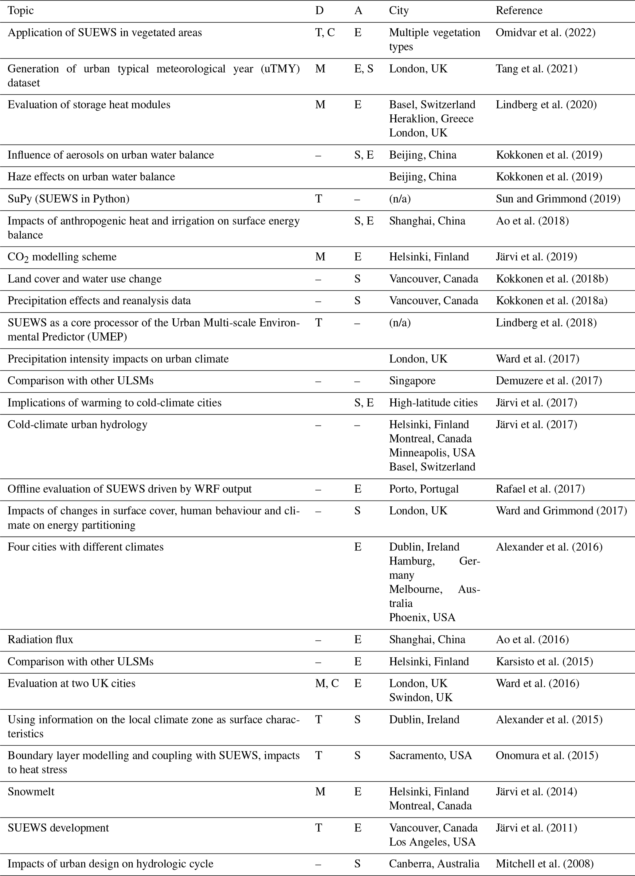
n/a: not applicable
Here, we couple SUEWS (v2018c; Sun et al., 2019) to the Weather Research and Forecasting (WRF) model (V4.0; Skamarock et al., 2019), an open-source frequently used NWP model. WRF provides the atmospheric forcing to SUEWS, and in turn WRF receives surface–atmosphere feedbacks for the city and the region. In this paper, we describe the structure and key physics of the coupled WRF–SUEWS system (Sect. 2), evaluate WRF–SUEWS at two UK sites (Sect. 3), and explore its application in modelling dynamics and impacts of anthropogenic heat emissions at the city scale (Sect. 4).
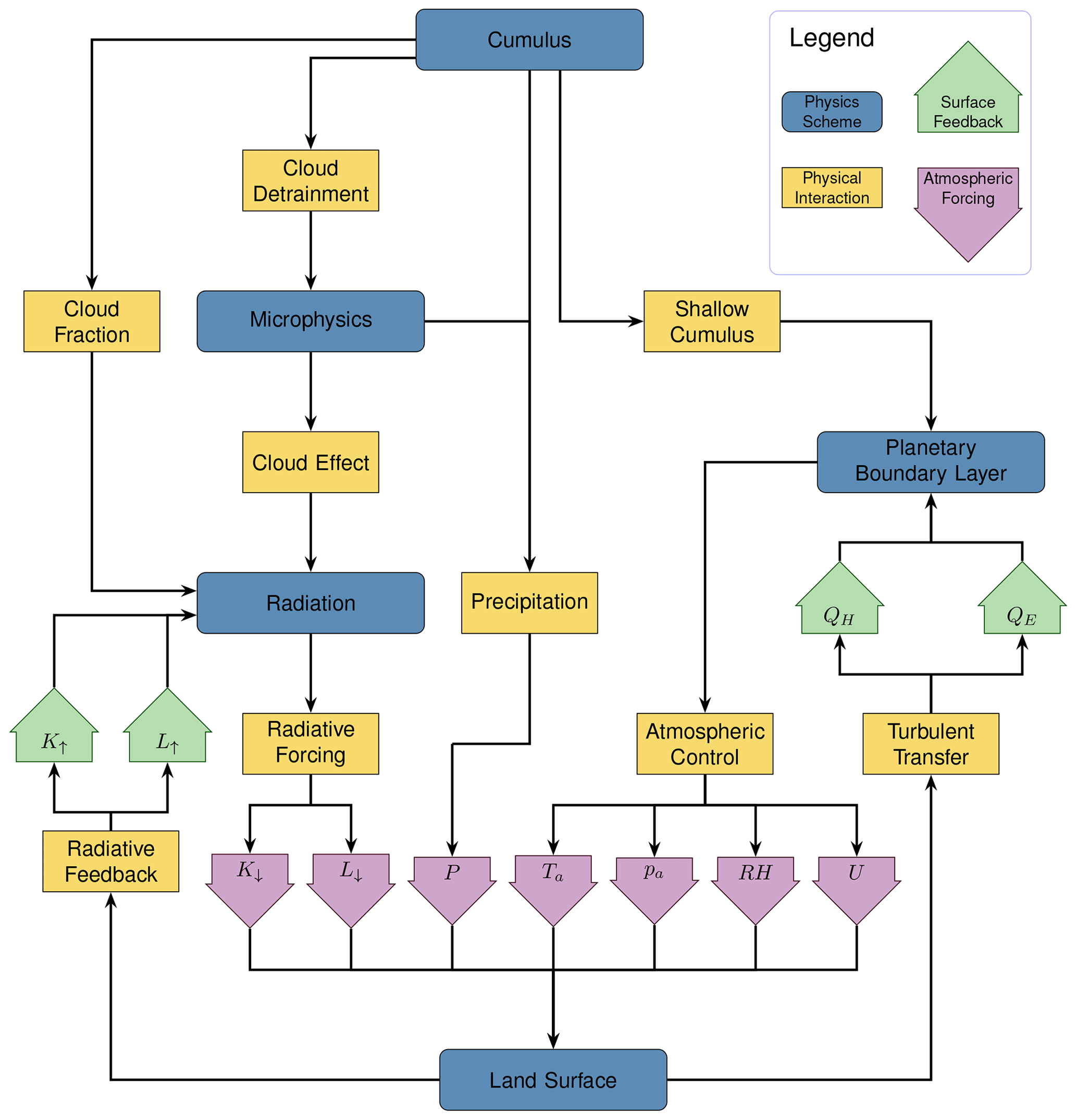
2.1 Physical interactions between WRF and SUEWS
The coupling between WRF and SUEWS occurs via the biophysical interactions between the land surface – with SUEWS introduced as a new land surface module option – and other physics modules in WRF (Fig. 1).
-
The radiation module provides radiative forcing variables, incoming short- (K↓) and long-wave radiation (L↓), to the land surface module. The land surface module returns outgoing short- and long-wave radiation (K↑ and L↑).
-
Atmospheric variables needed for SUEWS, including air temperature Ta, relative humidity RH, barometric pressure pa and wind speed U, are supplied by the boundary layer (BL) module. These are influenced by turbulent transport (i.e. momentum τ, sensible heat QH and latent heat QE fluxes) from the land surface.
-
Precipitation P is generated by the microphysics and cumulus modules that parameterise precipitation-related processes at different scales.
2.2 Key physics of SUEWS
SUEWS simulates both the energy balance (Oke, 2002),
and water balance (Grimmond et al., 1986),
The two are linked through the latent heat (QE) or evaporative E fluxes (by the latent heat of vaporisation). The water balance is driven by precipitation (P) and external water use (Ie). Whereas the surface energy balance is driven by the net all-wave radiation (, where K and L denote the short- and long-wave components, respectively, and arrows ↓ and ↑ in the subscript denote the incoming and outgoing directions, respectively) in all environments but additionally in cities, the human activities result in anthropogenic heat flux emissions (QF). The turbulent sensible (QH), latent (QE) and net storage heat flux (ΔQS); runoff (R); and change in water storage (ΔS) each have distinct responses that differ with land use and land cover. Traditionally, SUEWS has been mostly used for urban areas (Grimmond et al., 1986; Grimmond and Oke, 1991; Järvi et al., 2011; Ward et al., 2016), but for WRF–SUEWS it has been extended to non-urban contexts (Omidvar et al., 2022). Each model grid cell has up to seven land cover types (paved, buildings, deciduous trees, evergreen trees, grass/crops, bare soil and water) whose fractions and properties (e.g. height, albedo, leaf area index) can each vary between grid cells.
In WRF–SUEWS, QF is calculated using heating and cooling degree days (HDDs and CDDs) following the Sailor and Vasireddy (2006) approach:
where aF0,aF1 and aF2 are grid-specific coefficients. The grid population densities ρpop,t could be a daily mean (i.e. day and night) value (e.g. Ward et al., 2016) or capture the diurnal variations (e.g. Ward and Grimmond, 2017; Ao et al., 2018). Typically, for cities with strong commuting flows (e.g. London), QF and ρpop,t are larger in the central business districts (CBDs) during the day due to the commuting but are higher in residential areas at night. As using daily mean population density may bias QF and lose intra-daily variability (e.g. difference in large city centres between work-intensive and non-work periods), following other models (e.g. Allen et al., 2010) we divide the day into four periods (morning transition, day, afternoon transition and night). Day and night population densities are used in their respective periods, and their averages are used in both transition periods. The other parameter values can be derived from more detailed models that are not rapid enough for NWP (e.g. GQF, Iamarino et al., 2011; Gabey et al., 2018; DASH, Capel-Timms et al., 2020). ΔQS for each grid cell is calculated using the Objective Hysteresis Model (OHM) (Grimmond et al., 1991):
where t is the time, fi is the fraction of the area of each land cover type (i) and values are material-related coefficients for each land cover type that can vary with the grid cell (cf. Sect. 3.1). This approach allows for much more rapid calculation of this flux than other methods. QE is introduced to the Penman–Monteith equation (Grimmond and Oke, 1991):
where s is the slope of saturation vapour pressure curve, ρ is the density of air, cp is the specific heat capacity of air at constant pressure, V is the vapour pressure deficit, γ is the psychrometric “constant”, ra is the aerodynamic resistance for heat or water vapour, and rs is the surface or canopy resistance. Following Monteith (1965), assuming energy balance closure, QH is calculated as
With the latent heat of vaporisation (Lv) and Eq. (5) we obtain to link surface energy (Eq. 1) and water (Eq. 2) balance. R includes the runoff from individual surfaces, in channels and to groundwater. External water use (Ie) is estimated based on the automatic and/or manual irrigation or external application (e.g. street cleaning) as follows (Järvi et al., 2011):
where Airr is the area irrigated, faut is the fraction of Airr that is automatically irrigated, values are site-specific coefficients, Td is the daily mean temperature and tr is the number of days since the rain. The net change in the water storage ΔS (e.g. in soil, in waterbodies, on the surface) is determined at each time step as the change in each surface water state compared to the previous time step.
The aerodynamic resistance (ra) is calculated at first at the atmospheric level in WRF–SUEWS, where the wind speed (U) is determined (Fig. 1):
where zd is the zero plane displacement height (m), z0m (and z0v) is the roughness length for the momentum (and heat/water vapour), u is wind speed at height Zm, κ is the von Kármán constant (0.4) and ψm (and ψv) is the atmospheric stability functions for momentum (and water vapour). Stability is determined iteratively using the Obukhov length and initiated with a LUMPS-calculated (Grimmond and Oke, 2002) sensible heat flux taking the grid land cover fractions into account.
To compute the grid-integrated surface resistance (rs), its inverse, the surface conductance (gs), is used (Ward et al., 2016):
The mix of vegetation within the grid is taken into account by considering each vegetation type i with land cover fraction fi, the maximum conductance , leaf area index (LAIi), maximum LAI (LAImax,i) and the surface conductance parameter (GPFT) determined by plant functional type. Functions g(K↓), g(Δq), g(Ta) and g(Δθ) are related to how the environmental variables – downwelling short-wave (K↓) radiation, specific humidity deficit (Δq), air temperature (Ta) and soil moisture deficit (Δθsoil ) – control the surface resistance. These functions have the following forms (Ward et al., 2016):
where the G parameters are related to environmental controls indicated by subscripts K for solar radiation, q for the specific humidity deficit (“base” and “shape” for base value and curve shape, respectively), Ta for air temperature and θ for the soil moisture deficit. Table 2 gives the values used in the evaluation of the coupled WRF–SUEWS system (detailed in Sect. 3.2). is the maximum incoming short-wave radiation (1200 W m−2 used in this work); with TL and TH being the lower and upper limits for switching off evaporation, respectively ( ∘C and TH=55 ∘C); and ΔθWP is the wilting point (120 mm).
LAI varies with growing degree days (GDDs) and senescence degree days (SDDs) via (Järvi et al., 2011, 2014)
where the previous-day (subscript d−1) LAI is used with the base temperature corresponding to the initiation of leaf-off (TBase,SDD ) and leaf-on periods (TBase,GDD). The model also requires and for each vegetation type i.
SUEWS accounts for the running water balance of the multiple surface types. The water amount on the canopy of each surface (Ci) (Grimmond et al., 1991) determines the surface resistance between dry and wet by replacing rs in Eq. (5) with rss (Shuttleworth, 1978):
where W is a function of the relative amount of water present on each surface to its water storage capacity Si:
Kr depends on the aerodynamic and surface resistances,
where rb, the boundary layer resistance, is a function of friction velocity u* (Shuttleworth, 1983):
Equations (15)–(18) ensure that the surface resistance rss has a smooth transition from 0 s m−1 (a completely wet surface) to rs (a dry surface).
2.3 Major updates since SUEWS v2018c
This work presents a coupling framework and its evaluation using SUEWS v2018, ensuring consistency in internal physics with the offline version for the comparison later in Sect. 3.4. However we note that the coupling structure designed for WRF–SUEWS enables seamless upgrades to more recent SUEWS versions.
Current offline versions of SUEWS have options not in the coupled WRF–SUEWS system, including
-
CO2 fluxes for local-scale anthropogenic and biogenic urban–atmosphere exchanges (Järvi et al., 2019)
-
roughness sub-layer profiles for the diagnosis of air temperature, humidity and wind speed within the roughness sub-layer (Theeuwes et al., 2019; Tang et al., 2021)
-
2-D radiation profiles for solar and thermal-infrared radiation for multi-layer urban canopies (Hogan, 2019)
-
ESTM (elemental surface temperature method) for heat storage estimation using surface temperature and thermal properties (Lindberg et al., 2020).
2.4 Technical implementation of the WRF–SUEWS coupling
The following are considered in the design of coupled WRF–SUEWS system.
-
Performance. Given coupling with file-based IO (input–output) exchanges has unacceptable computational performance, we use the
SuMinmodule under the WRF framework (Figs. 2 and 3). -
Extendibility. As SUEWS is regularly enhanced (Table 1), it is desirable or even essential for the coupled system to use the full capacity of the standalone SUEWS.
-
Sustainability. Given the vast community effort to build and improve sophisticated software systems, coupling should not be limited to one version. Instead a highly standardised coupling procedure is required to be sustainable (Meyer et al., 2020).
To address these, the coupled WRF–SUEWS system uses an adaptive intermediate layer SuMin (SUEWS in minimum mode) to link both models (Fig. 5). From SUEWS, SuMin calls the main SUEWS calculator to conduct all core SUEWS physics calculations. Whereas from WRF, SuMin is linked to the module_sf_suews via suews_1d as a complete land surface model that can be used by the WRF dynamics solver (i.e. ARW solver; Advanced Research WRF) via the surface driver (Fig. 5). By coupling SUEWS and WRF this way, fast prototyping of new functionalities is possible on the SUEWS side while maintaining a stable coupling to the more complex WRF. When new SUEWS features are available to be fully coupled, appropriate switches can be activated to incorporate them within the whole WRF system. This intermediate-layer-based approach allows for efficient communication between SUEWS and other models (e.g. SuPy, Sun and Grimmond, 2019) through an explicit, unified interface. Thus, SUEWS can be potentially coupled to other weather/climate modelling systems (e.g. OpenIFS, ECMWF, 2021).
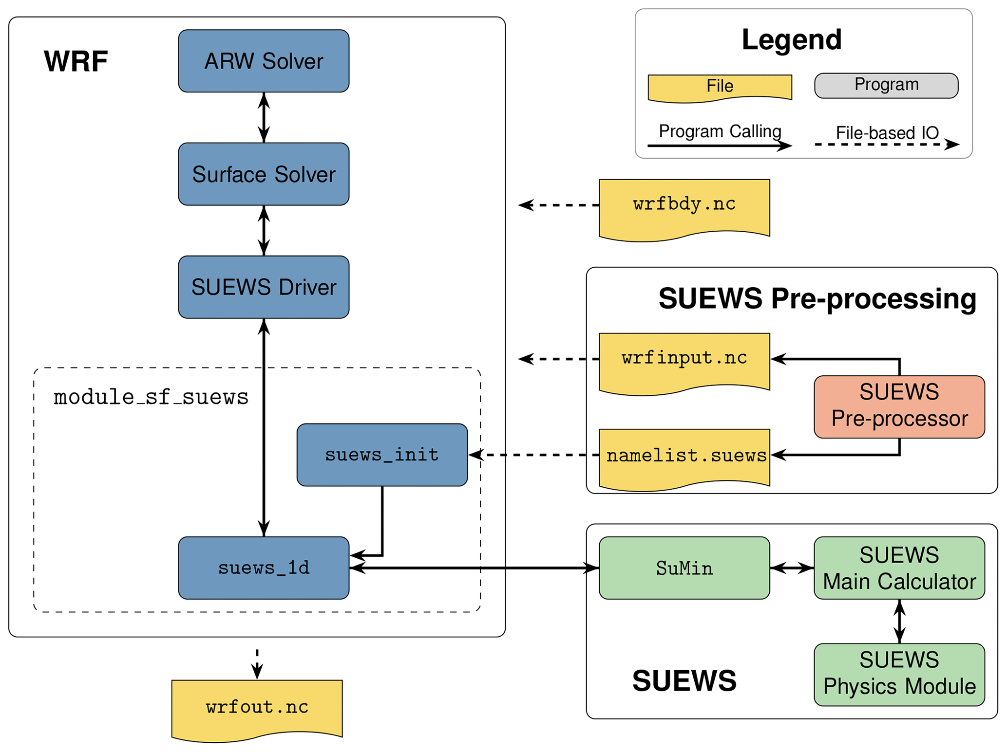
Figure 2WRF–SUEWS system consists of the new module_sf_suews added into WRF (blue) to interact with SUEWS via SuMin (green) using input files pre-processed by the SUEWS pre-processor (yellow). File-based input–output flow (dashed) and runtime calling logic (solid lines) are shown. suews_init is a subroutine to initialise the SUEWS module coupled into WRF, while wrfbdy.nc and wrfout.nc are standard WRF boundary condition and output files, respectively.
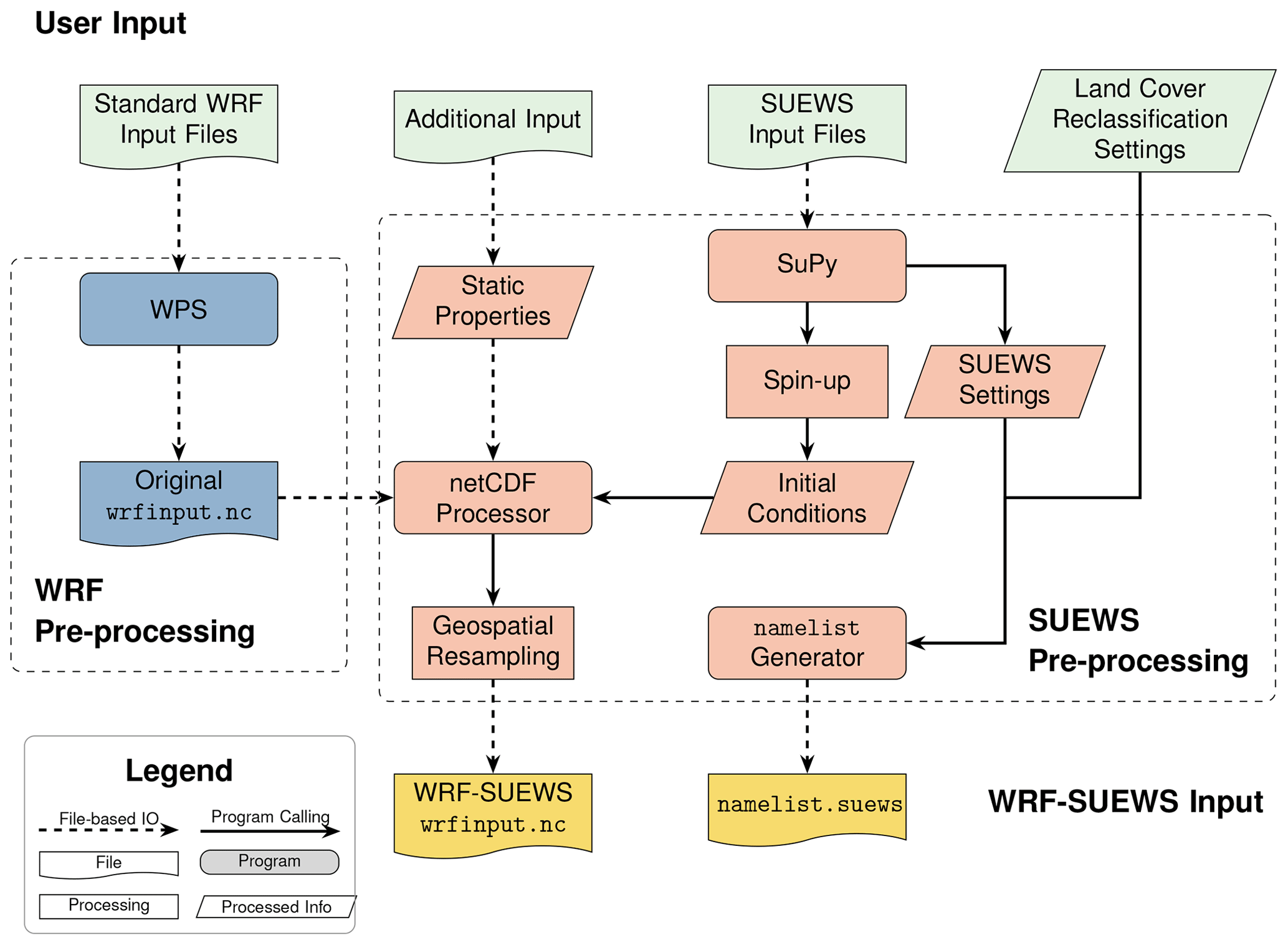
A Python-based WRF–SUEWS pre-processor system (WSPS; Fig. 5) formats the data to allow the additional parameters not in standard WRF input files (e.g. input variables in wrfinput.nc- and namelist-based configurations; cf. IO workflow in Fig. 3) to be incorporated, rather than modifying the WRF Pre-Processing System (WPS). The WSPS can be used for offline model spin-up runs to obtain the appropriate required initial conditions for WRF–SUEWS. The files prepared are
- i.
wrfinput.nc, which is a modified version of WRF inputs with initial model states and other static properties, and - ii.
namelist.suews, which is the global configuration for the SUEWS model.
To generate these, four types of inputs are needed (Fig. 3).
- i1.
Standard WRF input files for WPS. The geographic and meteorological data are processed by WPS to produce
wrfinput.ncfiles for the model domains and provide the template for the WSPS. - i2.
Additional input files. The static SUEWS-specific properties (e.g. land cover, population density, building morphology) and optional files (e.g. suitable default parameters to be used when known values are unavailable) will precede the same information, if available, in the standard WRF input files within the coupled WRF–SUEWS system. Note that in the London context this is not required (see later in Sect. 3).
- i3.
Standard SUEWS input files. These are files used by SuPy (Sun and Grimmond, 2019) for offline spin-up simulations to obtain appropriate model initial conditions (an example shown in Sect. 3.2). The SUEWS settings (e.g. physics options, population density profiles) are used to create the
namelist.suewsglobal settings. - i4.
Land cover reclassification settings. In
namelist.suewsthe relations between land covers for WRF and SUEWS (Sect. 2.4) are prescribed.
The WSPS input files (Fig. 3) can have different spatial resolutions between files. The implemented netCDF processor obtains the static properties (i2) and initial condition (i3) and resamples them to the geospatial configuration (projection method, resolution and averaging strategy) of the base wrfinput.nc (i1) to produce the wrfinput.nc files for WRF–SUEWS. Subsequently, namelist.suews can be easily modified by hand without going through the WSPS if useful (e.g. to test different configurations for spin-up or change land cover mapping relations).
The seven land cover (LC) types can be assigned different parameter values (Table 2) per grid cell and/or can change with time. For example, the “grass” vegetation type can have varying parameters by season (e.g. rice–wheat rotation). The WSPS uses the namelist.suews global configuration file to translate the WRF land use (LU) data, e.g. IGBP-modified (International Geosphere-Biosphere Programme) MODIS (Moderate Resolution Imaging Spectroradiometer) with 20 LU classes or the USGS with 24 LU classes (NCEP, 2000) to the 7 LC classes (Fig. 4). Each SUEWS LC may combine fractions from multiple IGBP LU classes. Through this reclassification, WRF–SUEWS can use existing LU data for SUEWS simulations while allowing the other parameters to vary between grids. Note that a flexible number of WRF LUs (up to 100 in this release) can be specified to compose a SUEWS LC so that an extremely heterogeneous LU composition can be accounted for.
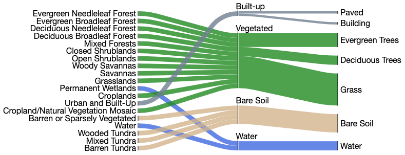
Figure 4The WSPS can be used to reclassify the WRF–IGBP default MODIS 20-category land uses to SUEWS-specific land covers: specifically, the 20 MODIS land use categories (left) with 4 general categories (middle) are reclassified into 7 SUEWS land covers (right).
2.5 Bulk-transmissivity-based solar radiation correction
Incoming short-wave radiation (K↓) is known to be overestimated by WRF because of unresolved clouds and/or aerosols (Jimenez et al., 2016; Lapo et al., 2017). However, if the forcing radiation is too large, the other surface fluxes and variables will be impacted. Thus, they should not compare well to observations, or alternatively if they do compare well, the variables are correct for the wrong reason. In urban areas, even on clear-sky days, there is often a large presence of aerosols that impact bulk transmissivities (e.g. Shanghai, Xu et al., 2011; Ao et al., 2018; Beijing, Dou et al., 2019; Sun et al., 2022; London, Ryder and Toumi, 2011; Kotthaus and Grimmond, 2018a; Warren et al., 2018). A bulk atmospheric transmissivity (τ) can be specified in the namelist.suews to partially correct the overestimation of K↓ by WRF, which can be determined using K↓ at both the top of atmosphere and the surface are used (Oke, 2002):
As τ can vary seasonally (e.g. the cases in London and Swindon as shown in Table 4) we determine the median clear-sky difference (Δτc) between τWRF and τobs from the analysis of clear-sky days observations around the peak K↓ (which occurs between 40 % and 60 % of the daylight hours). The K↓ forcing (Fig. 1) for SUEWS in WRF () is then corrected using the original one produced by WRF () as
Given the empirical nature of the parameter values, this correction can only be applied where observations are available. Here, we apply the correction to all time periods but separate the evaluation (Sect. 3.4.1) by sky conditions to assess effectiveness. Obviously, this simple correction is not a complete solution but rather an attempt to obtain more accurate K↓ forcing for the coupled SUEWS and, hence, better surface feedbacks for the WRF atmospheric modules (Fig. 1).
3.1 Surface characteristics of evaluation sites
WRF–SUEWS is evaluated at the same two UK sites as in a previous SUEWS evaluation study (Ward et al., 2016; W16 hereafter) for consistency – these sites exhibit distinct urban characteristics:
-
KCL. The King's College London Strand Campus (51∘30′ N, 0∘07′ W) is a dense central business district area in London (d03 of Fig. 5).
-
SWD. Swindon (51∘35′ N, 1∘48′ W) is a residential area in the town of Swindon (d04 of Fig. 5).
WRF–SUEWS is set up with four nested model domains (Fig. 5) with grid spacing (domain and number of grids) being 9 km (d01, 100×100), 3 km (d02, 115×91) and 1 km (d03 and d04, 76×76).
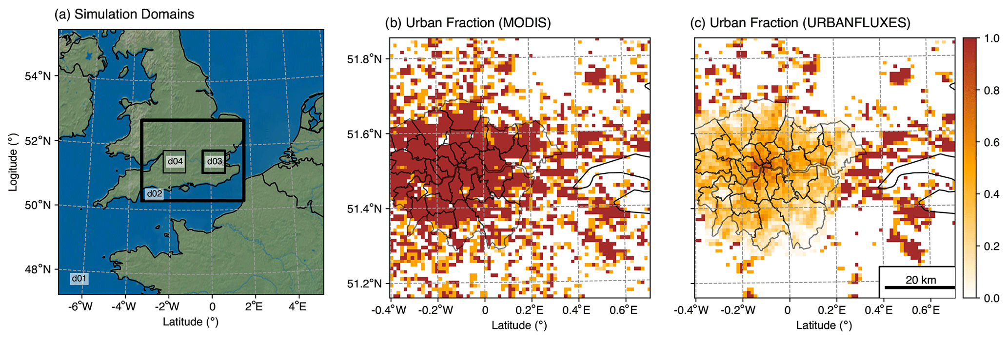
Figure 5Model domain configurations: (a) four simulation domains (d01–d04) and urban land cover (paved and buildings) fraction in d03 (1 km resolution) based on (b) the WRF default MODIS dataset and (c) updated information for Greater London from the URBANFLUXES project (Lindberg et al., 2020). The land cover information is accessible in Sun et al. (2023a).
As the default MODIS-based built (building and paved) fraction does not capture the surface heterogeneity within Greater London (Fig. 5b), we replace it with a high-resolution (i.e. 2.5 m) land cover map (Fig. 5c) derived from earth observation (EO) VHR (very high resolution) SPOT (Satellite pour l'Observation de la Terre) imagery (Mitraka et al., 2016; Marconcini et al., 2017) with more realistic surface information. This high-resolution dataset is processed using UMEP (Lindberg et al., 2018) to derive both land cover fractions for the seven SUEWS classes and other morphological parameters of roughness elements (e.g. building and vegetation heights, frontal area index; Table 2). The resulting dataset is upscaled to obtain 1 km resolution data for d03. As equivalent detailed land cover information is unavailable for d04, the land cover (plus building and vegetation height) for the single grid where Swindon site is located is modified based on values in Ward et al. (2016) (Table 2).
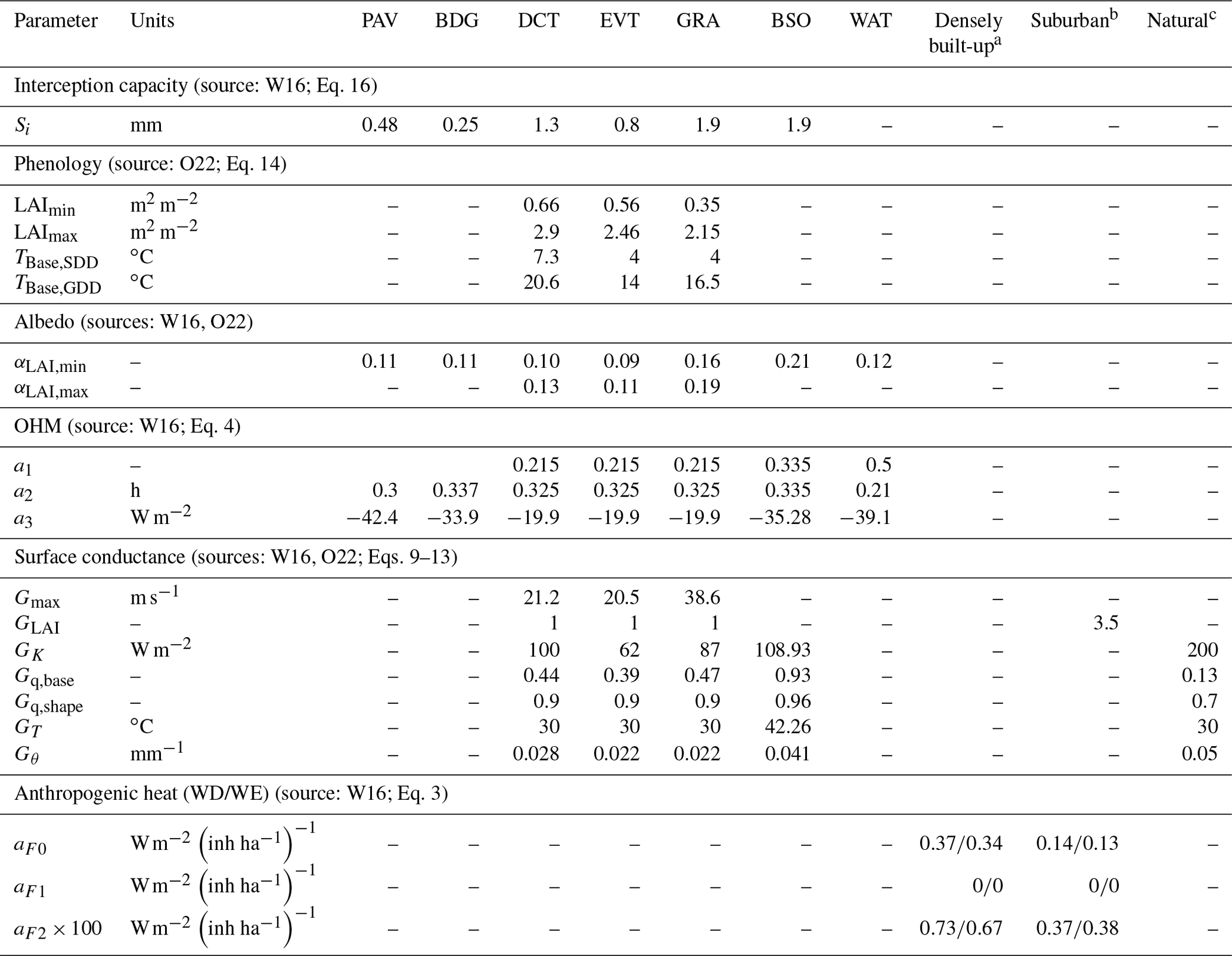
Table 2Key parameters assigned in the four model domains (Fig. 5) vary with land cover that is impervious (paved: PAV, buildings: BDG) and pervious (deciduous trees and shrubs: DCT, evergreen trees: EVT; grass: GRA, crops: CRP; bare soil: BSO, water: WAT). Anthropogenic heat flux coefficients vary between weekday (WD) and weekend (WE) periods. Data sources are Chrysoulakis et al. (2018) (C18), Lindberg et al. (2020) (L19), Omidvar et al. (2022) (O22) and Ward et al. (2016) (W16). Inhabitant: inh.
a . b . c .
To help assign SUEWS parameters related to the surface characteristics, the land cover characteristics of the 1362 d03 grid cells within Greater London are analysed by plan area fractions of paved (fPAV) and building (fBDG) land covers (Fig. 6). The most common (N=171) LC grid combination (i.e. fPAV−fPAV 0.05 fraction bins) is predominately pervious (notably grass) with minimal impervious area (<0.05 for both paved fPAV and buildings fBDG). The second most frequent (N=112, fPAV=0.15 and fBDG=0.1) is also largely pervious. It is also noting that KCL and SWD (blue dots in Fig. 6) reside in densely built-up and moderately pervious domains, respectively, indicating the different nature in land cover composition. Because high-resolution property information is not readily available across the evaluation domains, the surface-related SUEWS parameters (e.g. albedo, emissivity, OHM coefficients) are simplified into three classes based on the paved and buildings fraction (fPAV+BDG) from the gridded land cover (Table 2): (a) densely built areas (fPAV+BDG>0.6) are assigned parameter values of KCL (W16), (b) suburban areas () are assigned parameter values of SWD (W16) and (c) natural surfaces () are assigned parameter values based on dominant vegetation (Omidvar et al., 2022). In doing so, we can utilise the available property data to accurately represent surface heterogeneity. Note that the WRF–SUEWS system allows for grid cell level surface characteristic parameters assignment (e.g. SUEWS simulation of Greater London by Lindberg et al., 2020).
Given the importance of population density to anthropogenic heat emissions (Eq. 3), output area day- and nighttime population data (UK ONS, 2013) are resampled to 1 km resolution for d03. For the grid point of SWD in d04, the Ward et al. (2016) values are used; otherwise, zero anthropogenic heat emission is set with population density being zero.
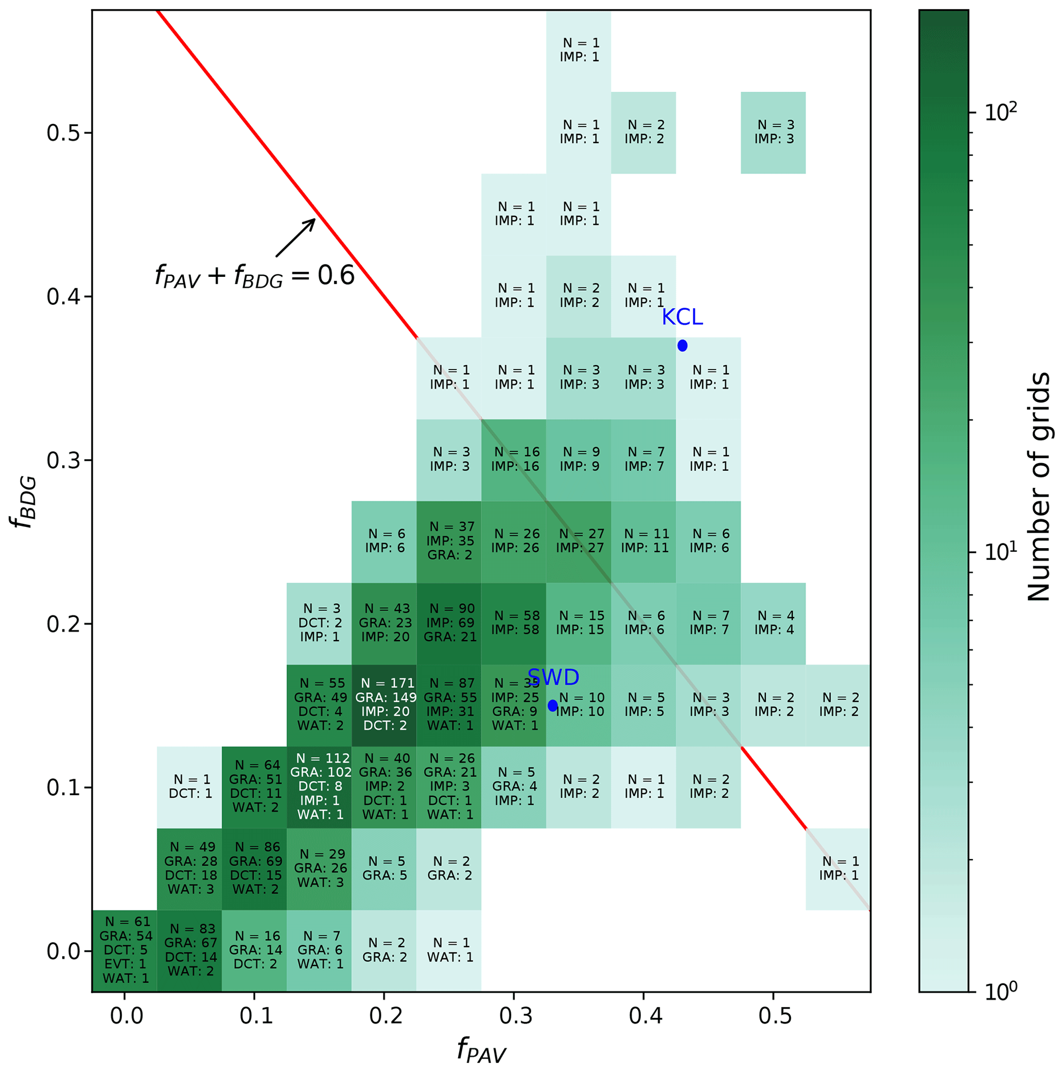
Figure 6Frequency (colour, N) of land cover characteristics in d03 (Fig. 5) for Greater London (GL) (1362 grids of 1 km2). The individual grid cells are categorised first by the greatest land cover fraction with an impervious (IMP) split between paved surfaces (PAV) and buildings (BDG). Other fractions are deciduous trees (DCT), evergreen trees (EVT), grass (GRA), bare soil (BSV) and water (WAT). The blue dots indicate the cover around the KCL and SWD evaluation sites.
3.2 Model setup and spin-up
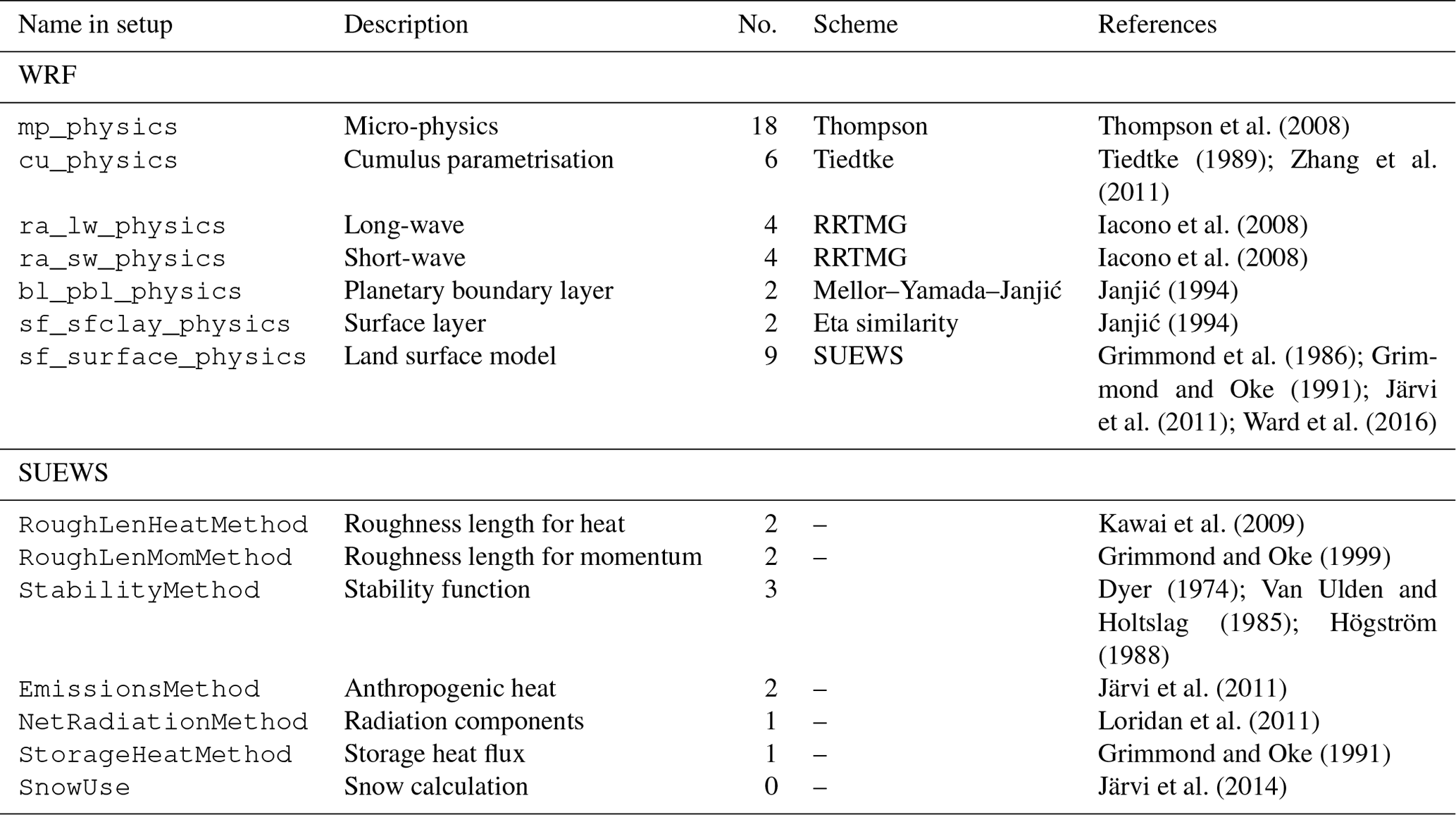
WRF–SUEWS is run with two-way nesting mode of 33 vertical levels (top at 5 kPa 11 layers in the boundary layer below 2000 m with lowest levels in d03 and d04 being ∼40 m a.g.l.; above ground level) for all four domains (Fig. 5). We note more vertical levels may be needed in detailed investigations of atmospheric features (e.g. temperature, precipitable water, etc.); here a moderate number of vertical levels are used as a balance between the computational cost and necessary representation of atmospheric profiles considering the focus of this work on the model development and evaluation of essential urban–atmosphere interactions. The atmospheric boundary conditions used are the 1∘ × 1∘ (latitude × longitude) National Centre for Environmental Prediction FNL (final) data (NCEP, 2000). The well-tested WRF “CONUS” (contiguous United States) physics suite (configuration since v3.9) is used with the land surface scheme changed to SUEWS (Table 3). The SUEWS physics schemes (Table 3, details provided in Sun et al., 2019) are selected for simplicity including using the building and tree heights with a rule-of-thumb method (Grimmond and Oke, 1999) for momentum roughness length and displacement height; additionally, snow and irrigation modules are turned off (following W16's KCL and SWD configuration). We use the WRF adaptive time step option to reduce the total run time while being numerically stable considering both the horizontal and vertical extent (Hutchinson, 2007). For us, the adopted time steps for domain 1 to 4 are around 72, 9, 3 and 3 s.
Thompson et al. (2008)Tiedtke (1989); Zhang et al. (2011)Iacono et al. (2008)Iacono et al. (2008)Janjić (1994)Janjić (1994)Grimmond et al. (1986); Grimmond and Oke (1991); Järvi et al. (2011); Ward et al. (2016)Kawai et al. (2009)Grimmond and Oke (1999)Dyer (1974); Van Ulden and Holtslag (1985); Högström (1988)Järvi et al. (2011)Loridan et al. (2011)Grimmond and Oke (1991)Järvi et al. (2014)Table 3Physics scheme in the WRF and SUEWS option tested for use in coupled simulations. The local (internal) option number is given in the column labelled “No.” RRTMG: Rapid Radiative Transfer Model for GCMs (general circulation models).
We evaluate WRF–SUEWS during the four seasons using 2-week periods in 2012 (Table 4). To generate appropriate initial conditions (i.e. model spin-up), we conduct offline SUEWS runs driven by observations collected at KCL and SWD (refer to the purple boxes in Fig. 1 and related notations in Sect. 2.2 for details about the atmospheric forcing variables as well as Table 2 for surface property settings) for 2012 until the soil moisture converges (<0.1 % difference in last time step between consecutive years): a period of 15 years is needed for KCL, while a period of 5 years is needed for SWD. For fully vegetated grids (i.e. fDCT/EVT/GRA=1), the observations at SWD are used as forcing conditions to spin-up SUEWS for 4 years before convergence. The required initial states (i.e. soil moisture, leaf area index) are used for each WRF–SUEWS period (Table 4). For grid cells with fPAV+BDG>0.6, the KCL-based initial states are prescribed to represent areas dominated by impervious surfaces, while SWD is used for the rest that are not completely vegetated. The appropriate complete pervious cover type values are assigned to the pervious cells based on their dominant land cover type.
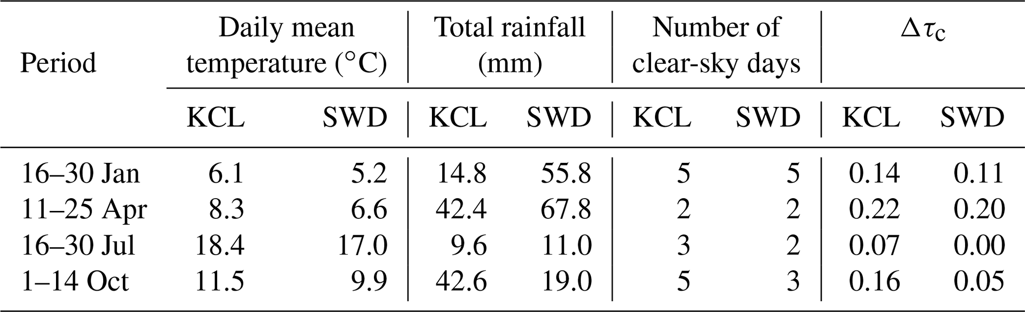
Table 4Time periods in 2012 used to evaluate WRF–SUEWS (Sect. 3.2) in London (KCL) and Swindon (SWD) with the observed air temperature (KCL at 49.6 m a.g.l., SWD at 10.6 m a.g.l.) and rainfall. Measurement details are given in Ward et al. (2013) and Kotthaus and Grimmond (2014a, b). Note that daylight saving time impacts all except for the January period; i.e. people's activities (e.g. work times) are 1 h earlier than UTC. Δτc is the median clear-sky transmissivity difference between τWRF and τobs. The clear-sky days are determined with a mean of τobs>0.8.
3.3 Evaluation data and metrics
The W16 evaluation of SUEWS (v2016a) uses 60 min radiation and turbulent fluxes observed at KCL and SWD (Ward et al., 2013; Kotthaus and Grimmond, 2014a, b). Both flux towers are located close to the centre (within a 200–300 m radius circle) of a 1 km2 model grid cell. The source areas of the observed turbulent fluxes have a probable 50 % contribution from within ∼400 m of the flux tower at KCL (Kotthaus and Grimmond, 2014b) and a probable 80 % contribution from within ∼700 m at SWD (Ward et al., 2013). Here, we average the 30 min sample output from land surface scheme (i.e. SUEWS) to 60 min to compare with the observations.
The mixed-layer height (MLH), derived from continuous high-resolution (15 s and 10 m) attenuated backscatter observed with a Vaisala CL31 ceilometer at Marylebone Road (MR) in London (Kotthaus et al., 2016; Kotthaus and Grimmond, 2018a, b), is used to evaluate the model's ability to predict atmospheric boundary layer (ABL) dynamics. The MLH values have been compared to AMDAR, or Aircraft Meteorological Data Relay (the median difference between inversion heights and MLH is 346 m based on all time periods; for more evaluation results, refer to Kotthaus and Grimmond, 2018a). Various observations can be used to obtain the height of the boundary layer, but the results depend on the variable used (Kotthaus et al., 2023). For example, differences occur between using temperature inversion and MLH (e.g. at night, Kotthaus and Grimmond, 2018a) or between MLH and the turbulence-derived mixing height (MH; Kotthaus et al., 2018), the height where the vertical velocity variations falls below a threshold (Barlow et al., 2011; Halios and Barlow, 2017). On the other hand, when using the Mellor–Yamada–Janjić scheme, the WRF output PBLH (planetary boundary layer height) is derived from the height where turbulent kinetic energy falls below 0.2 m2 s−2 (Banks et al., 2016; Janjić, 1994).
Although the comparison of the aerosol-derived MLH from observations and the turbulence-based mixing height diagnosed from the model output (WRF PBL, hereafter referred to as WRF MH) may be affected to systematic differences (e.g. those associated with vertical resolution as suggested by Kotthaus et al., 2023), the comparable nature between MLH and MH enables the former to be a proxy to examine the latter modelled by WRF.
The evaluation metrics used with the number of data points (N) available from the model output (Ymod) and observation (Yobs) time series are the following.
-
Hit rate (HR).
with Heaviside step function H defined by
and the threshold δY,j being a value dependent on evaluation variable Y. We use the HR to evaluate the surface energy fluxes with δYj=50 W m−2 for radiative and for turbulent (QE and QH) fluxes (Hollinger and Richardson, 2005), respectively. If HR=0, it suggests none of model predictions are within the acceptable threshold set, while HR=1 indicates all fall into the acceptance range.
-
Mean absolute error (MAE).
-
Mean bias error (MBE).
Both the MAE and MBE have units of the variable analysed (i.e. W−2 for fluxes, m for MLH or MH) with an ideal value of 0 indicating perfect agreement with the observations. The MAE, unlike the root mean square error, treats all error equally (Willmott et al., 2017).
3.4 Evaluation results
3.4.1 Effect of bulk transmissivity correction on solar radiation
First, we evaluate WRF–SUEWS' skill at predicting incoming short-wave radiation (K↓) as it is crucial to driving surface–atmosphere processes (Fig. 1). Given that fixing WRF's RRTMG radiation scheme (Iacono et al., 2008) tendency to overestimate K↓ is beyond the scope of this study, we modify K↓ for each grid to ensure that the land surface receives the appropriate energy to drive the land surface scheme (e.g. SUEWS) by accounting for the differences in bulk transmissivity on clear-sky days (Fig. 7; correction methodology in Sect. 2.5).
Generally, after the correction is applied the modified K↓ agrees better with observations on clear-sky days (Fig. 8) with reduced overestimation. The improvement in the HR is minimal, but the MAE and MBE become smaller. This type of correction may cause underestimation of the peak K↓ values in summer (Fig. 8c; cf. Fig. 8g), as the WRF overestimated transmissivity is larger in the afternoon (Fig. 7). Thus using a single bulk correction will have a diurnal bias in K↓ from undercorrection (overcorrection) in the morning (afternoon). This is evident in the ascending trend of ΔτSim-Obs (cf. Fig. 7).
On cloudy days, the correction also improves the K↓ performance. The MAE and MBE, as well as the HR, are enhanced, despite the correction parameter not being derived for cloudy conditions (Fig. 9). The MBE is reduced by more than 50 % for all simulation periods at both sites (except October 2012 at SWD) after correction. In general, we deem such correction necessary and effective for land surface modules in the WRF system (v4.0); hence we use K↓-corrected simulation results throughout the following analyses.
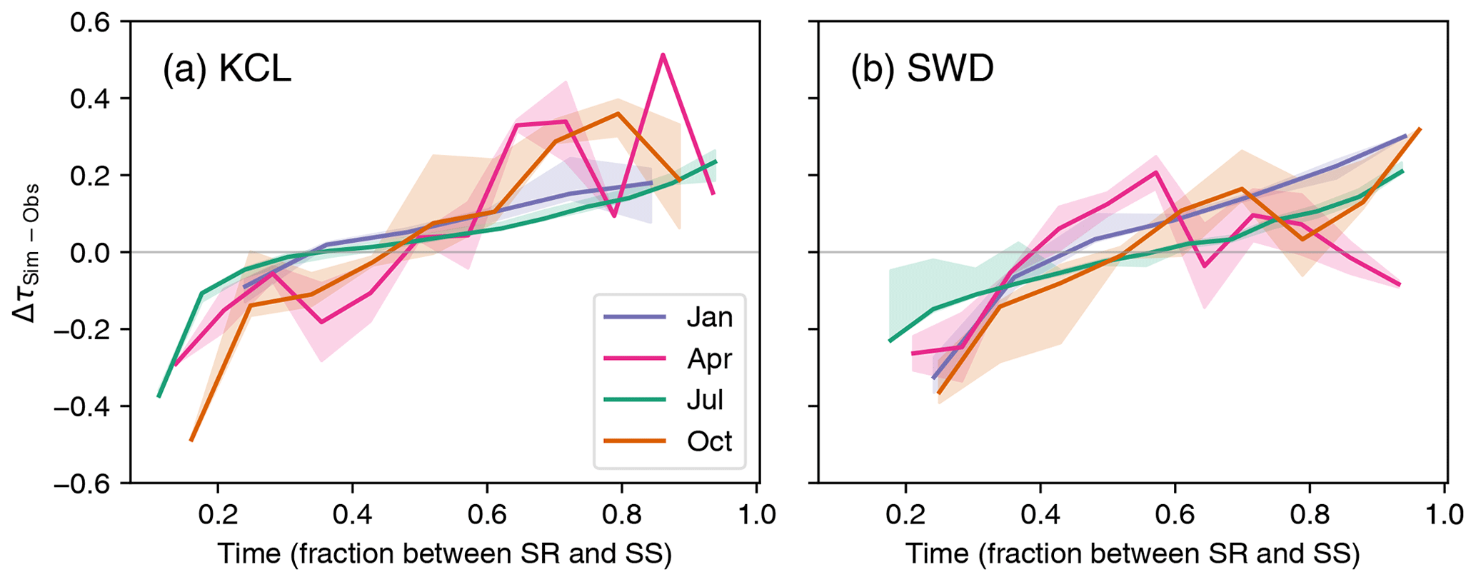
Figure 7Bulk transmissivity difference (model − observation) of 60 min median values (line) and the interquartile range (shading) during the daylight hours (normalised between sunrise (SR: 0) and sunset (SS: 1)) during four periods of the year (Table 4) at (a) KCL and (b) SWD. See Sect. 2.5 for correction details of Δτ.
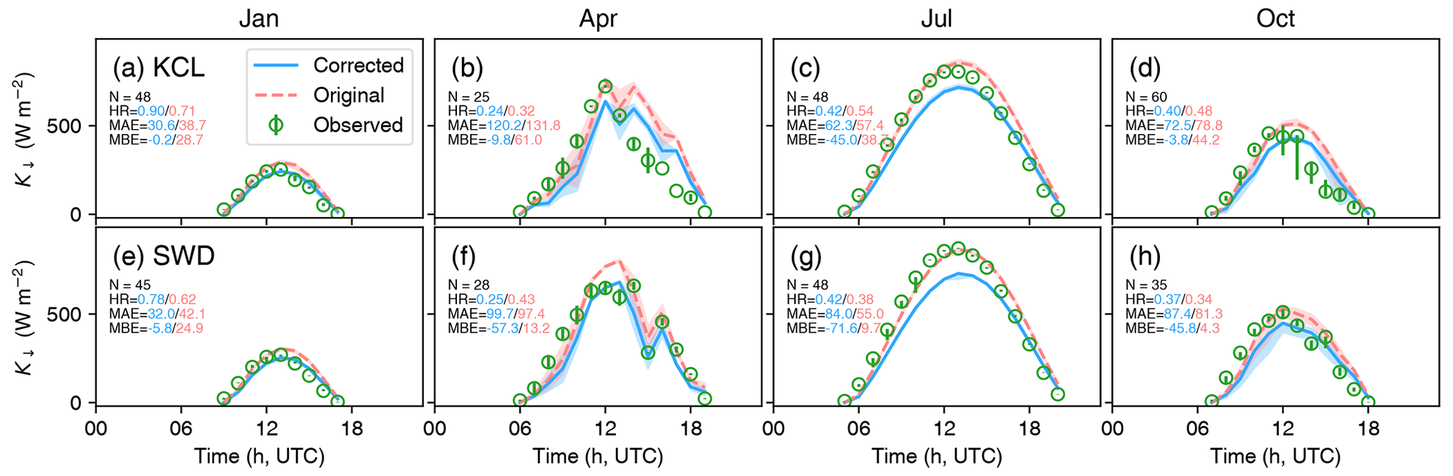
Figure 8Daytime 60 min incoming short-wave radiation (K↓) fluxes during clear-sky days. Observed data are marked with median values (circles) and the interquartile range (IQR, vertical lines), while simulations by WRF–SUEWS are illustrated with median values (lines) and the interquartile range (shading). Both the original (solid) and corrected bulk transmissivity (dashed) are utilised across four 2-week periods (refer to Table 4) at the (a–d) KCL and (e–h) SWD sites. Scarce clear-sky periods occurred in April. For additional details on metrics and units, refer to Sect. 3.3.
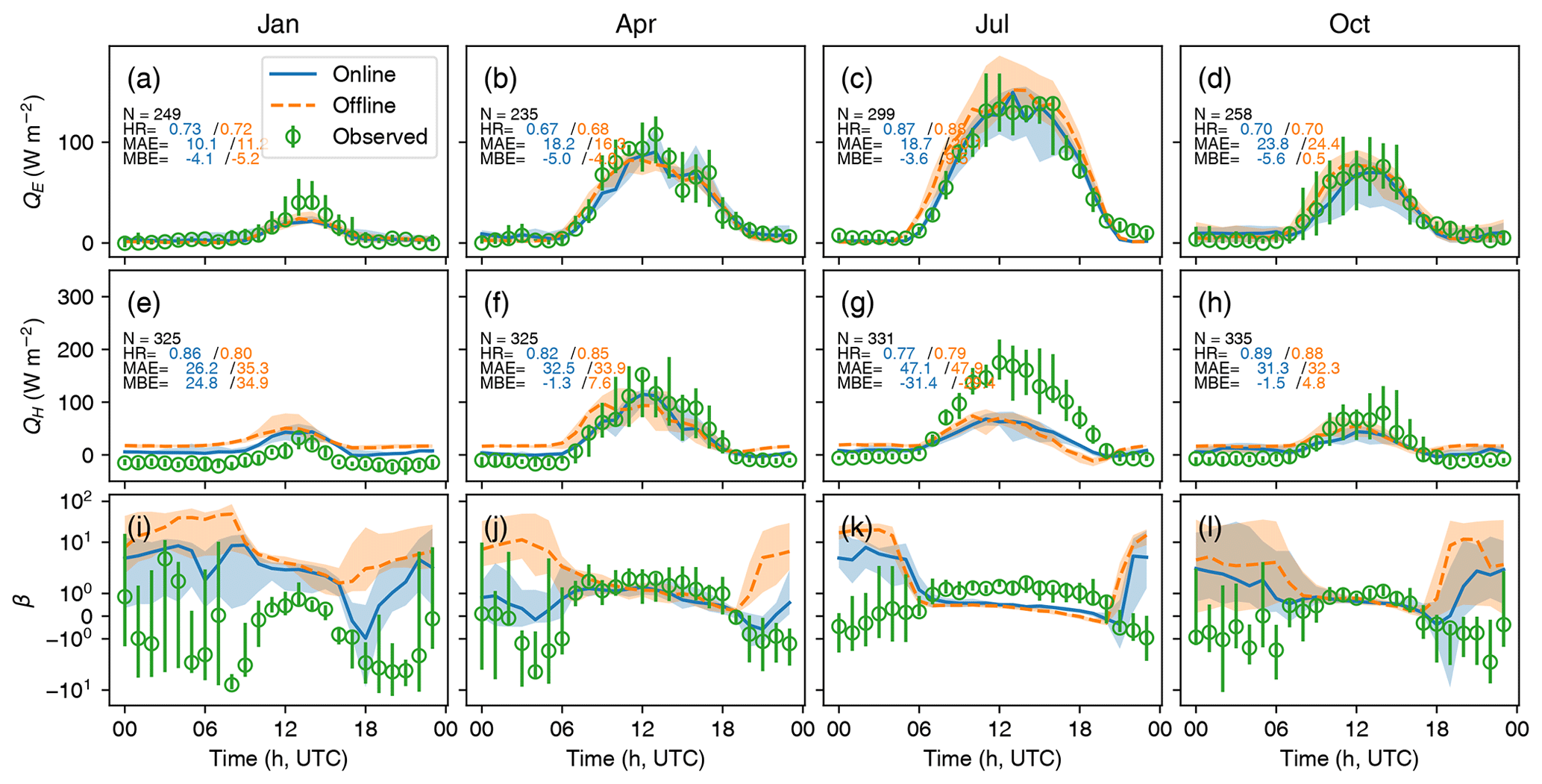
3.4.2 Online and offline simulated surface energy balance fluxes
Although our focus is on the online WRF–SUEWS system, it is useful to compare its performance to the offline (i.e. standalone SUEWS) version. As we force the latter directly with observations (refer to the “atmospheric forcing” variables in Fig. 1), removing potential forcing errors from the online system, we expect better performance and hence use this as a benchmark. The same simulation periods were used for the online and offline evaluation (Table 4). Given that the SUEWS v2018c kernel is almost the same as the v2016 kernel, the offline performance is very similar to the values reported by W16. The largest difference may be associated with an update to the OHM calculations, as v2016 uses the mean net all-wave radiation values of the 2 preceding hours, while v2018c uses the step-size-weighted average of two successive time steps.
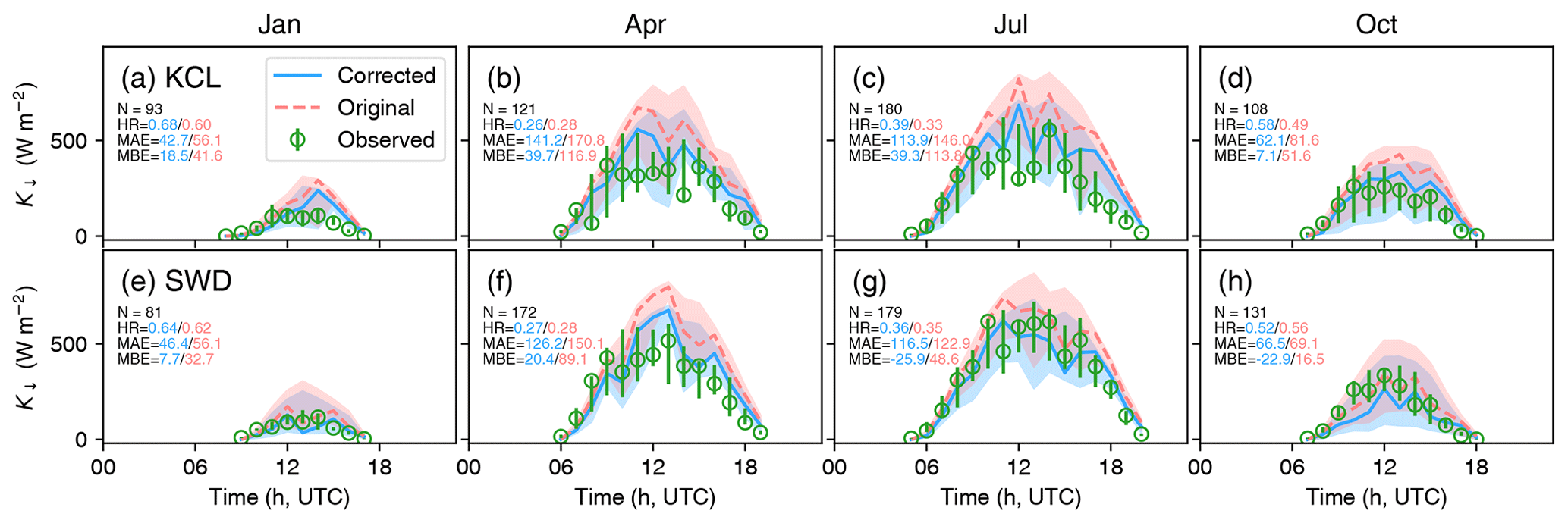
Overall, the offline (upper row, Fig. 12) performance is better than online (lower row) at both sites for all fluxes. Although offline K↓ should have no error, slight deterioration in performance occurs (Ward et al., 2016) because the high-resolution (e.g. 1, 5 min) forcing is not used but rather 60 min means are interpolated to 5 min and subsequently re-averaged to 60 min for evaluation. The offline K↓ HR is greater than 0.93 for all four seasons at both sites, whereas the online K↓ HR values are 0.25 to 0.75 (Figs. B1–B2) with HR<0.5 and MAE >60 W m−2 in April and July (Fig. 12). The model performance in K↑ is comparable at both sites (Fig. 12); the offline mode proves to be superior to the online mode – this is not surprising as it corresponds to the model's performance in K↓.
The outgoing long-wave radiation L↑ is modelled well (MAE <12.6 W m−2) both offline and online. But like K↓, L↓ is poorer for both cases (MAE online: 28.6; offline: 28.2 W m−2) and its diurnal patterns is quite captured by the model correctly – the offline mode lacks sufficient diurnal variability, while the online mode shows general underestimation (cf. Figs. 10, 11). Net all-wave radiation (Q*) is impacted mostly by K↓ during the day, making the WRF K↓ correction important. The intra-annual range of the MAE for the online Q* simulations is smaller for KCL (21–64 W m−2) than at SWD (37–72 W m−2), so the turbulent fluxes at SWD start with a potentially greater error.
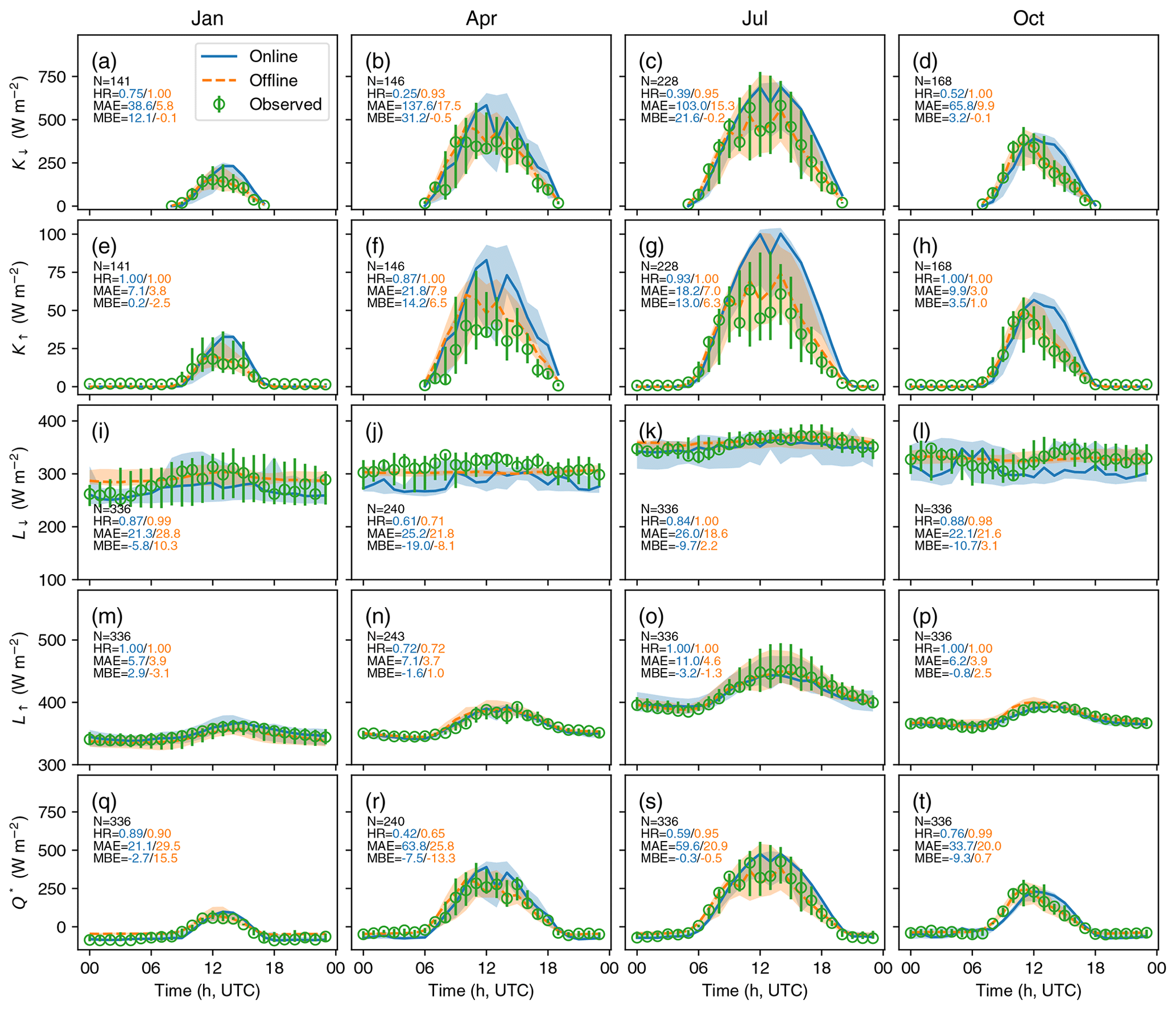
Figure 10Diurnal pattern of simulated (median: online – solid, offline – dashed; IQR: shading) and observed (median: circle, IQR: vertical line) incoming (a–d) short-wave (K↓) and (e–h) long-wave (L↓), outgoing (i–l) short- (K↑) and (m–p) long-wave (L↑), and (q–t) net all-wave (Q*) radiation for four 2-week periods in different seasons (Table 4) at KCL. “N” indicates the number of hourly data points used in the analysis; other metrics are defined in Sect. 3.3.
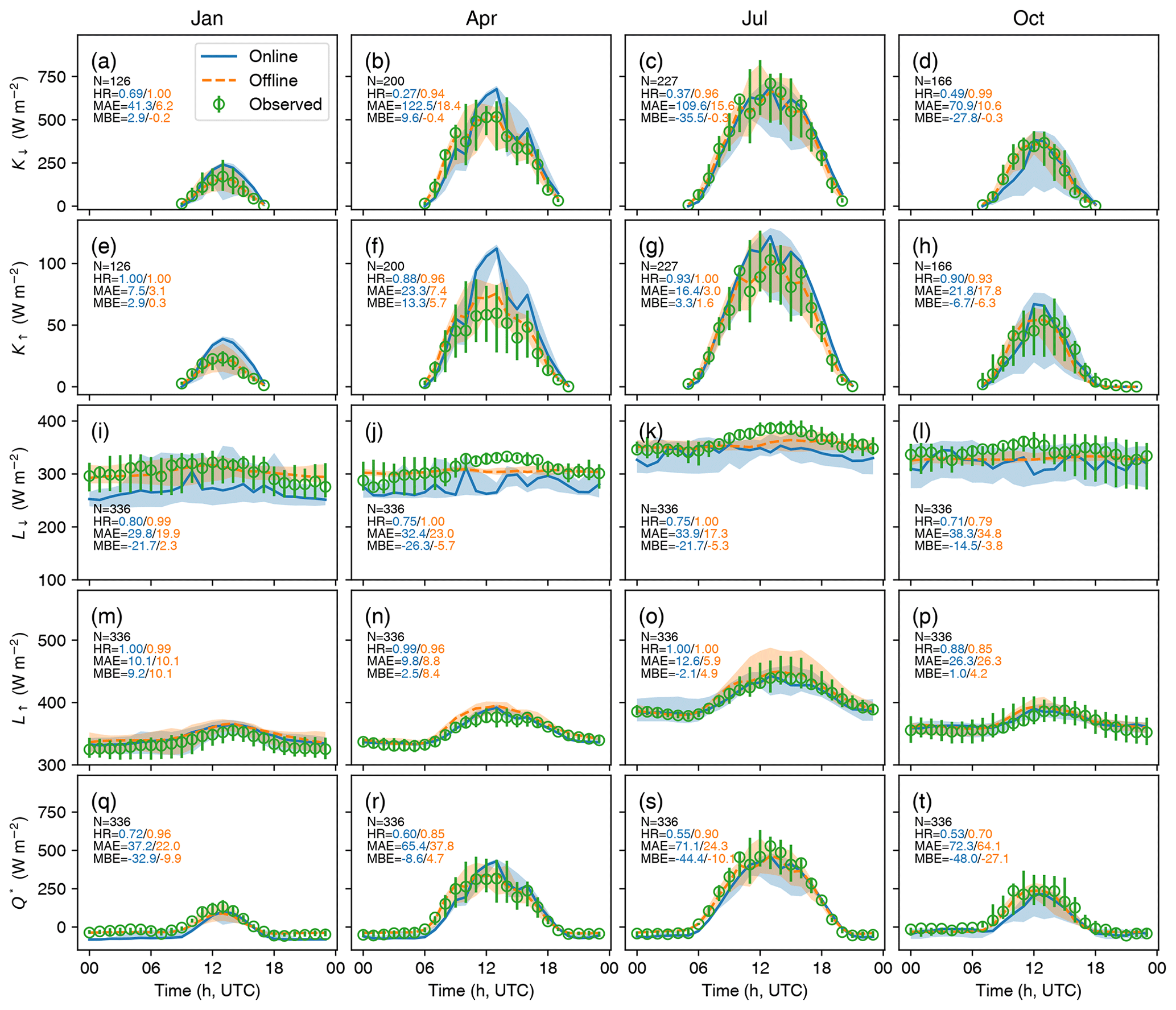
Clear-sky seasonality in the MBE for the turbulent heat fluxes (QE and QH) occurs at both sites (Fig. 12). At KCL there is a positive bias of varying magnitude (6 to 47 W m−2) for both fluxes, whereas at SWD QE is generally underestimated (−6 to −4 W m−2) and QH is overestimated (underestimated) by 25 W m−2 (−31 W m−2) in January (July).
Overall, WRF–SUEWS better predicts QE than QH at both sites ( vs. : 26 vs. 45 W m−2 at KCL and 18 vs. 62 W m−2 at SWD). The diurnal performance for the turbulent heat fluxes and Bowen ratio is similar for both offline and online runs for both KCL and SWD (Figs. 13, 14). The β indicates the turbulent heat fluxes are correctly partitioned, suggesting the model's robustness in turbulent heat flux partitioning even when there are variations in radiation accuracy (i.e. making the skill in simulating the absolute radiation fluxes less critical). The WRF–SUEWS daytime β agrees well with the observations at both KCL and SWD. However, when both fluxes are small (<10 W m−2) there are both larger observational errors (e.g. uncertainties due to nocturnal weak turbulence; Järvi et al., 2018; Mahrt et al., 2012) and ratios change rapidly. Under these conditions, the nocturnal β is overestimated (January at KCL; all seasons at SWD).
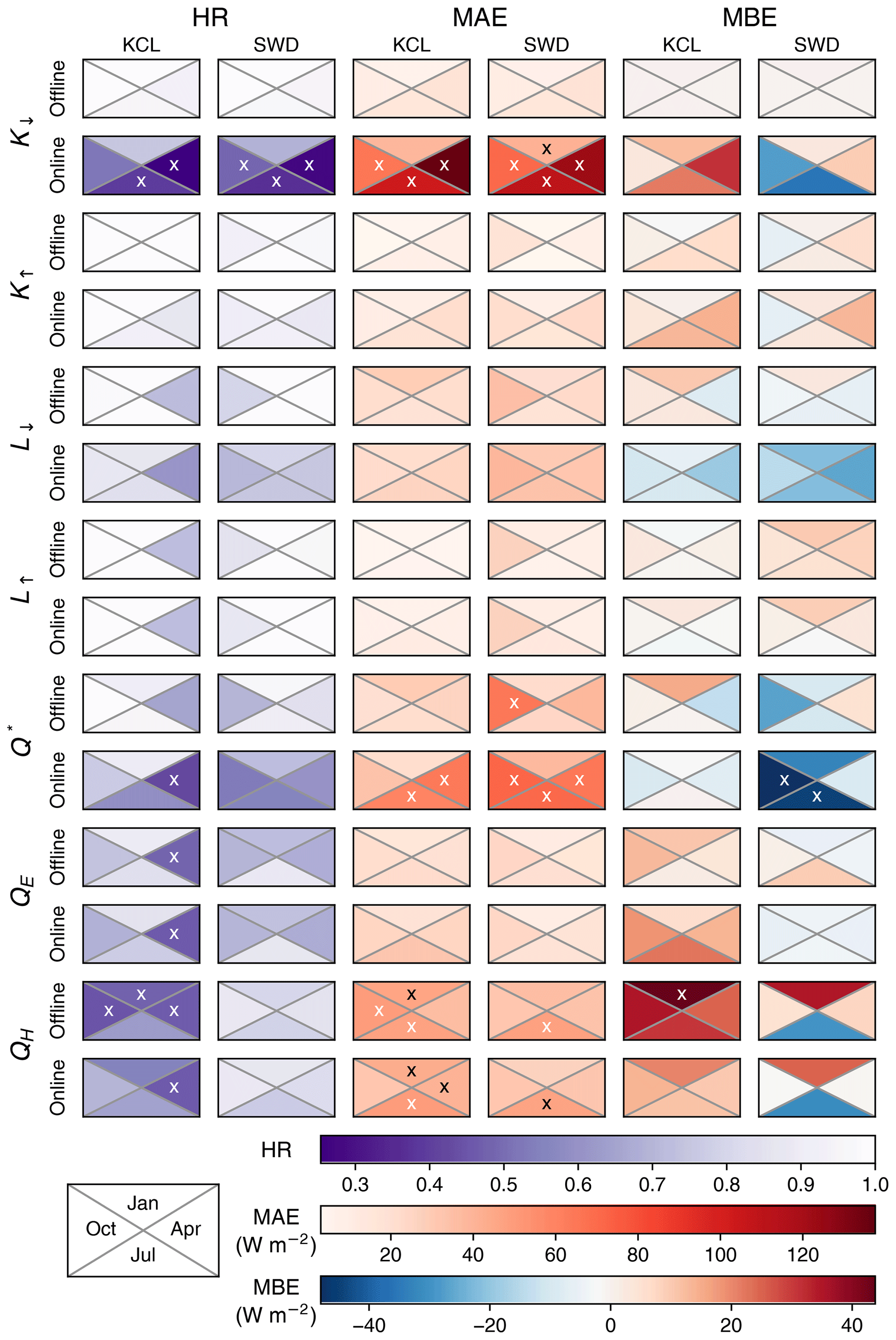
Figure 12Model performance for (rows) radiative and Q*) and turbulent heat (QE and QH) fluxes for (rows) simulated online and offline modes at (columns) KCL and SWD assessed using (columns) three metrics (HR, MAE, MBE: colour – darker for poorer performance) for four periods (triangles). Triangles marked × indicate the model performance can be categorised unsatisfactory based on the one of following criteria: HR<0.5, MAE>40 W m−2 and W m−2. Metrics are defined in Sect. 3.3.
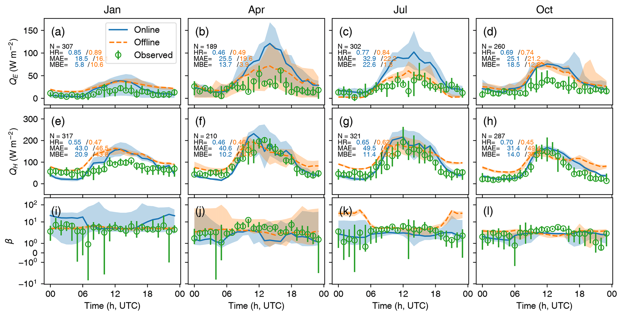
Figure 13Diurnal pattern of simulated (median: online – solid, offline – dashed; IQR: shading) and observed (median: circle, IQR: vertical line) fluxes: (a–d) sensible (QH) and (e–h) latent (QE) heat fluxes and (i–l) Bowen ratio (hourly median) for (columns) four 2-week periods in different seasons (Table 4) at KCL. Metrics defined in Sect. 3.3.
To set these results into context, it is useful to compare them to the results of other urban land surface models that have been evaluated in this region (e.g. SLUCM, Loridan et al., 2013; Tsiringakis et al., 2019; Best-1T and MORUSES with JULES, Hertwig et al., 2020). Loridan et al. (2013) (hereinafter L13) focussed on 3 June 2010 using KCL observations to evaluate the SLUCM (Kusaka et al., 2001) in WRF (Chen et al., 2011). Hertwig et al. (2020) (H20) evaluated two urban schemes with JULES (Best et al., 2011), Best-1T (Best et al., 2006) and MORUSES (Porson et al., 2010), over the 2011–2013 period at both the KCL and SWD sites. The evaluation strategies differ: L13 considers both online and offline performance but with different surface information; H20 is offline only but considers a range of configurations. For comparison we consider their more “advanced” configurations (L13: online, UZE – Urban Zones for Energy partitioning – for plan-area-index-based surface categorisation; H20: offline, a baseline configuration, CTRL-B, and a more sophisticated one, CTRL-M, with the more realistic anthropogenic forcing and detailed land cover information) using appropriate periods.
WRF–SLUCM performance at KCL for QE is better (WRF–SUEWS MAE=33 W m−2); note that the L13 study covers only 1 d (cf. our summer of 14 d). Similar to SUEWS, SLUCM's online mode performs slightly worse than its offline mode with respect to RMSE (online vs. offline), 82.8 vs. 82.6 W m−2 for QH, while for QE, it is 16.4 vs. 14.2 W m−2. At KCL, the annual offline MAESUEWS for QE is similar to CTRL-B but larger than CTRL-M , whereas all three model configurations have similar performance at SWD . For QH, all three models are similar at KCL , but at SWD, MAESUEWS is larger than for the two H20 models .
Although not directly comparable, the SUEWS performance appears to be consistent with both offline and online performance of other urban land surface models in this area. Attribution of bias differences (e.g. different parameterisations, configurations, land cover information) is out of the scope of this study but is the focus of model comparison studies (e.g. Grimmond et al., 2010a, b).
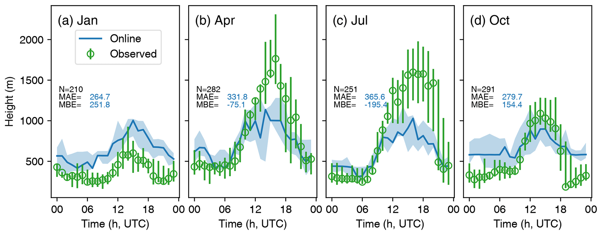
3.4.3 Boundary layer depth
To assess the boundary layer depth the modelled MH (Sect. 3.3) is compared to the observed MLH at MR in London (Fig. 15). Generally, WRF–SUEWS underestimates daytime MH in all seasons except for winter (Fig. 15a) with MAE>300 m in the warmer periods (Fig. 15b, c). WRF–SUEWS slightly overestimates MH at night. The MBE varies between −195 and 252 m for the four periods. These values are smaller than WRF–SLUCM (with multiple PBL schemes, −288 to 539 m) simulations over Greater Paris evaluated using radiosonde observations (Kim et al., 2013). Similarly, evaluating WRF using eight different PBL schemes in Barcelona, Banks et al. (2015) found daytime MH to be underestimated (cf. elastic backscatter lidar), with the largest relative bias of −48 %. This is comparable to our summertime results (Fig. 15c).
4.1 Modelled variability in anthropogenic heat emissions
The WRF–SUEWS model demonstrates satisfactory performance across various seasons and for two distinct urban areas (Sect. 3.1). Therefore, we employ it to examine the influence of QF on the atmospheric boundary layer – a unique characteristic of the coupled WRF–SUEWS system compared to the standalone SUEWS – in d03 (Fig. 5) during April 2012, before the Olympics disrupted typical patterns in July. As daylight saving time has begun by this time of the year, people's activities are shifted an hour earlier (e.g. typical workday is 08:00–16:00 UTC or 09:00–17:00 BST local time; British summer time). Peak QF emissions occur in central London (Fig. 16) during the daytime (, Fig. 16c). By the late afternoon and through the night (20:00–05:00 UTC) the values in these areas (Fig. 16b) are smaller (, Fig. 16d). The areas where large values occur differ between night and day.
At night the peaks occur across a larger area beyond central London, with some larger values towards the outskirts (Fig. 16b; cf. Fig. 16a). The nocturnal QF mean in d03 is smaller (17.1 W m−2) than the daytime (19.8 W m−2) but is more spatially consistent (Fig. 16d; cf. Fig. 16c).
These spatiotemporal patterns (Fig. 16a, b) are largely consistent with previous studies in London. Daily peak values differ between studies because of model grid cell size (Lindberg et al., 2013) and efforts over time to reduce carbon emissions and therefore energy use (Lindberg et al., 2013; Ward and Grimmond, 2017). Peak values (grid size) vary between 120 W m−2 (3.2 km2, Capel-Timms et al., 2020), (1 km2, Hamilton et al., 2009; 1 km2, Bohnenstengel et al., 2013) and 210 W m−2 (3.2 km2, Iamarino et al., 2011). Besides, the WRF–SUEWS-predicted average QF values for London (i.e. ) are comparable with those estimated in other mega-cities (e.g. peak values of in the city of Osaka, Japan, by Narumi et al. (2009); annual average of in the Beijing–Tianjin–Hebei agglomeration by Feng et al. (2012); annual average of in Beijing by Yang et al. (2022)).
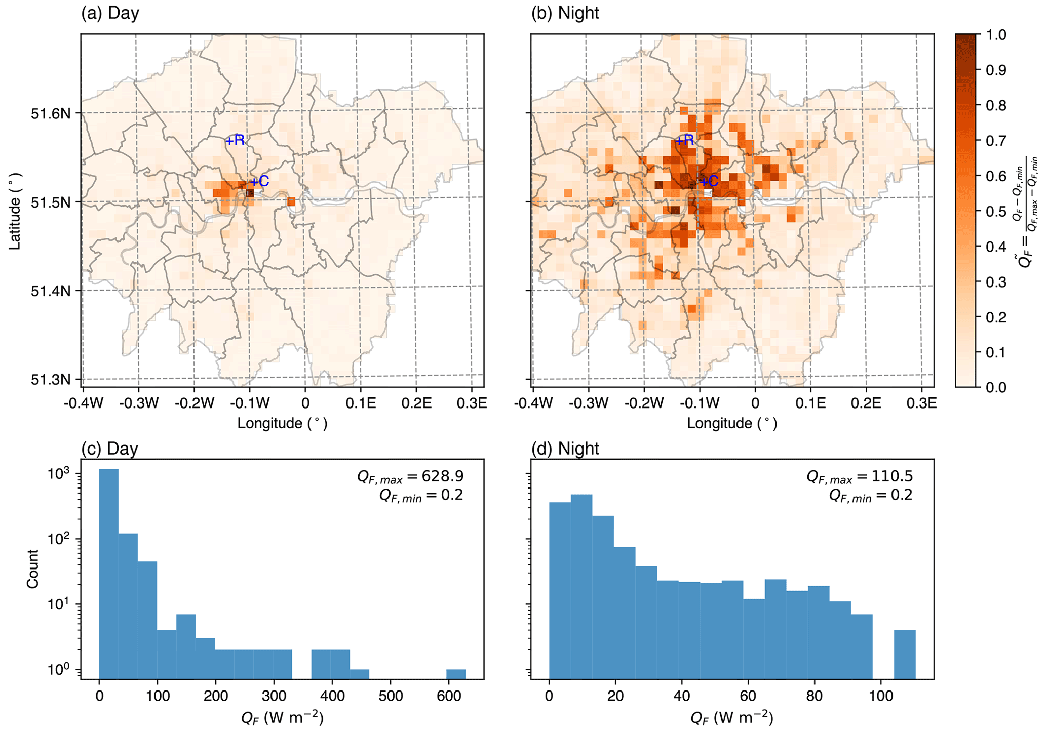
Figure 16April (Table 4) weekday normalised anthropogenic heat flux in London (grey lines are boroughs) (a) during main working hours in the day (08:00–16:00 UTC) and (b) at night (20:00–05:00 UTC), with (c, d) the respective distributions of their actual values (in W m−2). Grids analysed in more detail are indicated (blue): commercial–business (C) and residential (R).
4.2 Feedbacks from anthropogenic heat emissions
To assess the feedback, we focus on two example grids with contrasting population density profiles:
-
a central business district (CBD) area, within the City of Westminster (grid C, Fig. 16), with tall buildings (roughness length z0=2.0 m, zero plane displacement zd=13.9 m; calculated using the rule-of-thumb approach as in Grimmond and Oke, 1999), a low fraction of vegetation (fVEG=13.1 %) and large daytime population density (763 inh ha−1) but small nocturnal density (111 inh ha−1)
-
an inner-city residential area, within the Borough of Islington (grid R, Fig. 16), with z0=0.8 m, zd=5.6 m, fVEG=43.3 % and nocturnal population density (170 inh ha−1) slightly greater than the daytime density (150 inh ha−1).
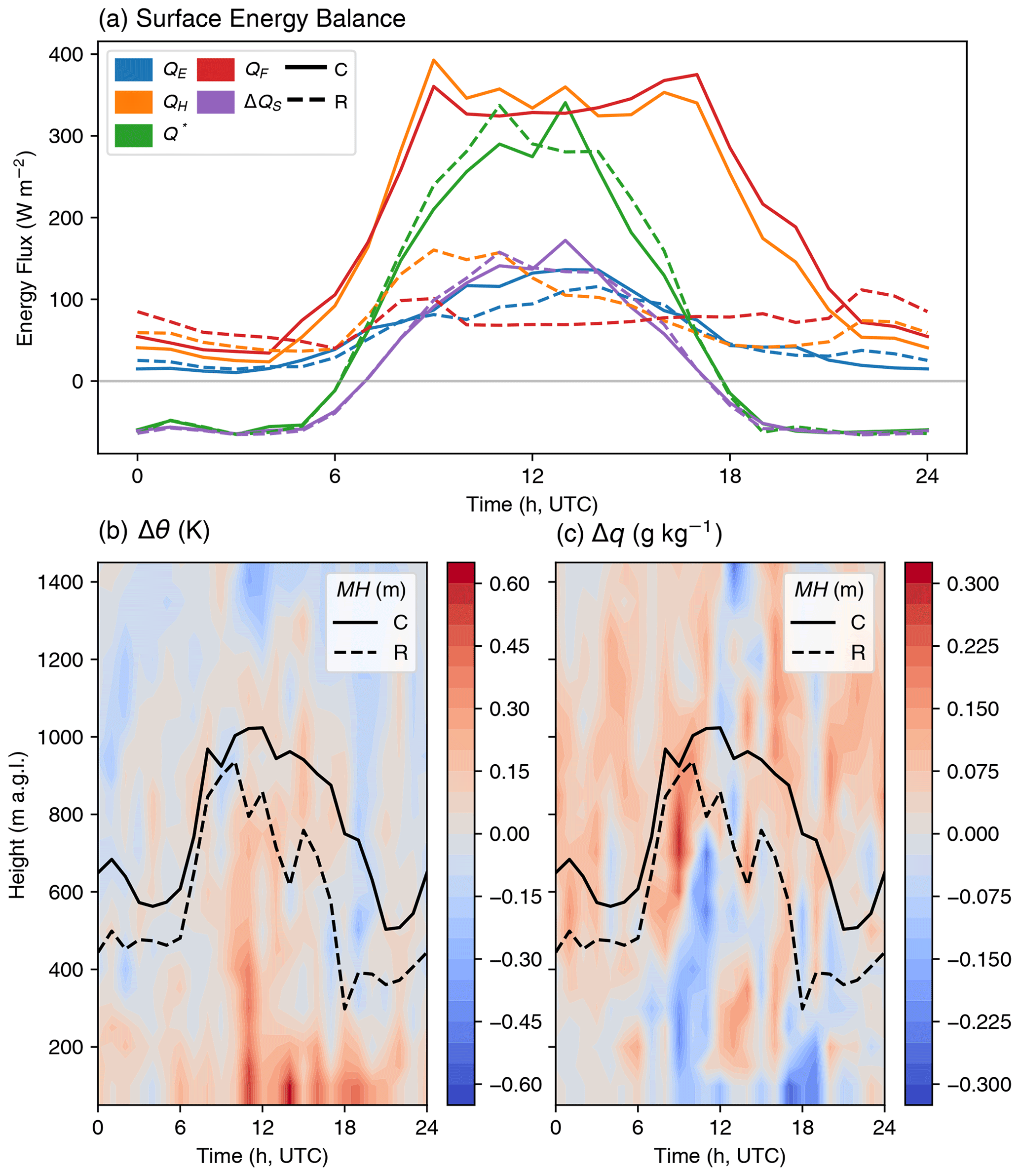
Workday time series reveal differences in QF timing and magnitude between the two grids (Fig. 17a). In grid C, QF is significantly higher in general, staying at a rather consistent level between the morning and evening peaks, whereas the flux is lower in grid R and shows a reduction in emission between the two peaks. However, the second peak in R is much later (R at ∼21:00 UTC, C at ∼17:00 UTC, Fig. 17a, red). Both grids have similar QE (Fig. 17a) despite the 30 % difference in vegetation fraction, attributable to the low LAI in April (Kotthaus and Grimmond, 2014a, b; Ward et al., 2013). The net radiation (Q*, Fig. 17a) values are also similar. The larger QF in grid C enhances QH by ∼220 W m−2 over grid R during the middle of the day on average, which contributes to an increase in midday MH of 100–200 m compared to grid R (700–900 m a.g.l.; Fig. 17b, c).
The contrasting QF-induced heating alters several atmospheric variables within the urban boundary layer: daytime near-surface air in grid C is warmer (positive difference, ∼0.3 K, Fig. 17b) and drier (negative difference, , Fig. 17c) than in grid R. At night, the air temperature in grid C stays warmer at lower altitudes but with cooler and wetter air aloft with PBL (Fig. 17). These results are consistent with other WRF–SLUCM-based studies stating that urban heating leads to warmer and drier near-surface atmosphere (e.g. Zhang and Chen, 2014; Zhang et al., 2015). The QF impacts are of similar magnitude to those linked to urban greening (but with an inverse effect): for instance, with all roofs vegetated in Beijing, the near-surface atmosphere is cooled by ∼1 K but moistened by during a heat wave period even when anthropogenic heat is accounted for (Sun et al., 2016); this suggests that urban greening may help mitigate some effects of anthropogenic heat emissions.
Through coupling the SUEWS urban land surface model to WRF, urban–atmosphere interactions can be explored more fully than when using the standalone SUEWS. The new Fortran subroutine SuMin interfaces SUEWS with the land surface driver of WRF. The WSPS pre-processor incorporates SUEWS-specific parameters into the wrfinput.nc and namelist.suews files for WRF–SUEWS simulations. The coupling is designed to permit sustainable development of SUEWS so that regular enhancements of SUEWS can be seamlessly incorporated into the coupled system.
Evaluation of the coupled WRF–SUEWS system is performed at two UK sites: dense central London (KCL) and a suburban–residential site in Swindon (SWD) across four seasons. It generally shows a good capacity of the coupled system to simulate the surface energy balance fluxes and mixing height in all periods. The performance compares well to other WRF studies in urban settings (Banks et al., 2015; Kim et al., 2013; Loridan et al., 2013). Better performance is found (i) at the suburban site SWD compared to the densely built-up KCL for the turbulent heat fluxes, (ii) during clear-sky conditions for radiative compared to turbulent heat fluxes and (iii) using a bulk atmospheric transmissivity for incoming short-wave radiation (compared to without).
WRF–SUEWS' capability allows for analyses of spatial and temporal variations over heterogeneous urban areas compared to existing WRF urban schemes (e.g. SLUCM, BEP, etc.) that can only resolve a limited number of urban classes. Critically, the SUEWS capability allows for dynamic feedbacks from human activities (e.g. heat, water, phenology, snow related). The influence of anthropogenic heat QF on the boundary layer in April prior to leaf growth in Greater London influences the sensible (more than the latent) heat fluxes. The larger QF and QH in central London are associated with warmer and drier air and deeper mixing heights during the day but not at night. The WRF–SUEWS evaluation should be expanded to other urban settings, time frames and synoptic conditions, with further applications being explored (e.g. QF impacts on urban–atmosphere interactions). Results suggest that the system has a great potential to help advance our understanding of the role of urban surface heterogeneity. As SUEWS is already integrated with many other models (e.g. building energy parameterisations and thermal comfort simulations, Table 1), WRF–SUEWS can help decision-makers involved in a wide range of integrated urban services to identify the spatiotemporal distribution of near-surface meteorology (e.g. heat-induced climate risks, Zong et al., 2022; urban ventilation issues, Zheng et al., 2022) across a city.
The snapshots of input data and source code for WRF–SUEWS used in this paper have been archived on Zenodo at https://doi.org/10.5281/zenodo.7957903 (Sun et al., 2023a) and https://doi.org/10.5281/zenodo.8137708 (Sun et al., 2023b), respectively. The up-to-date version of WRF–SUEWS is available at https://github.com/Urban-Meteorology-Reading/WRF-SUEWS (last access: 16 May 2023).
TS led the development of WRF–SUEWS with significant contributions from HO and ZL. TS and HO performed the evaluation. TS, HO and SG drafted the manuscript, and all authors reviewed and edited the manuscript.
The contact author has declared that none of the authors has any competing interests.
Publisher's note: Copernicus Publications remains neutral with regard to jurisdictional claims made in the text, published maps, institutional affiliations, or any other geographical representation in this paper. While Copernicus Publications makes every effort to include appropriate place names, the final responsibility lies with the authors.
This work has been supported by the Newton Fund–Met Office Climate Science for Service Partnership (CSSP) China (HighResCity, grant no. AJYG-DX4P1V), the Natural Environment Research Council (independent research fellowship, grant nos. NE/P018637/1 and NE/P018637/2; COSMA, grant no. NE/S005889/1; ClearfLo, grant no. NE/H003231/1; studentship, grant no. NE/H52479X/1), the European Research Council (Synergy, urbisphere, grant no. 855005; FP7, BRIDGE, grant no. 211345) and the National Natural Science Foundation of China (grant no. 41975006). Helen C. Ward is supported by the Austrian Science Fund (grant nos. M2244-N32 and V888-N).
This research has been supported by the Natural Environment Research Council (grant nos. NE/P018637/1, NE/P018637/2, NE/S005889/1, NE/H003231/1 and NE/H52479X/1), the European Research Council (FP7 Ideas, grant nos. 855005 and 211345), the National Natural Science Foundation of China (grant no. 41975006), the Newton Fund–Met Office Climate Science for Service Partnership (CSSP) China (HighResCity, grant no. AJYG-DX4P1V) and the Austrian Science Fund (grant nos. M2244-N32 and V888-N).
This paper was edited by Jatin Kala and reviewed by two anonymous referees.
Alexander, P., Bechtel, B., Chow, W., Fealy, R., and Mills, G.: Linking urban climate classification with an urban energy and water budget model: Multi-site and multi-seasonal evaluation, Urban Clim., 17, 196–215, https://doi.org/10.1016/j.uclim.2016.08.003, 2016. a
Alexander, P. J., Mills, G., and Fealy, R.: Using LCZ data to run an urban energy balance model, Urban Clim., 13, 14–37, https://doi.org/10.1016/j.uclim.2015.05.001, 2015. a
Allen, L., Lindberg, F., and Grimmond, C. S. B.: Global to city scale urban anthropogenic heat flux: Model and variability, Int. J. Climatol., 31, 1990–2005, https://doi.org/10.1002/joc.2210, 2010. a
Ao, X., Grimmond, C. S. B., Liu, D., Han, Z., Hu, P., Wang, Y., Zhen, X., and Tan, J.: Radiation Fluxes in a Business District of Shanghai, China, J. Appl. Meteorol. Clim., 55, 2451–2468, https://doi.org/10.1175/jamc-d-16-0082.1, 2016. a
Ao, X., Grimmond, C. S. B., Ward, H. C., Gabey, A. M., Tan, J., Yang, X.-Q., Liu, D., Zhi, X., Liu, H., and Zhang, N.: Evaluation of the Surface Urban Energy and Water Balance Scheme (SUEWS) at a Dense Urban Site in Shanghai: Sensitivity to Anthropogenic Heat and Irrigation, J. Hydrometeorol., 19, 1983–2005, https://doi.org/10.1175/jhm-d-18-0057.1, 2018. a, b, c
Baklanov, A., Grimmond, C., Carlson, D., Terblanche, D., Tang, X., Bouchet, V., Lee, B., Langendijk, G., Kolli, R., and Hovsepyan, A.: From urban meteorology, climate and environment research to integrated city services, Urban Clim., 23, 330–341, https://doi.org/10.1016/j.uclim.2017.05.004, 2018. a
Banks, R. F., Tiana-Alsina, J., Rocadenbosch, F., and Baldasano, J. M.: Performance Evaluation of the Boundary-Layer Height from Lidar and the Weather Research and Forecasting Model at an Urban Coastal Site in the North-East Iberian Peninsula, Bound.-Lay. Meteorol., 157, 265–292, https://doi.org/10.1007/s10546-015-0056-2, 2015. a, b
Banks, R. F., Tiana-Alsina, J., Baldasano, J. M., Rocadenbosch, F., Papayannis, A., Solomos, S., and Tzanis, C. G.: Sensitivity of boundary-layer variables to PBL schemes in the WRF model based on surface meteorological observations, lidar, and radiosondes during the HygrA-CD campaign, Atmos. Res., 176-177, 185–201, https://doi.org/10.1016/j.atmosres.2016.02.024, 2016. a
Barlow, J. F., Dunbar, T. M., Nemitz, E. G., Wood, C. R., Gallagher, M. W., Davies, F., O'Connor, E., and Harrison, R. M.: Boundary layer dynamics over London, UK, as observed using Doppler lidar during REPARTEE-II, Atmos. Chem. Phys., 11, 2111–2125, https://doi.org/10.5194/acp-11-2111-2011, 2011. a
Best, M. J. and Grimmond, C. S. B.: Key Conclusions of the First International Urban Land Surface Model Comparison Project, B. Am. Meteorol. Soc., 96, 805–819, https://doi.org/10.1175/bams-d-14-00122.1, 2015. a
Best, M. J., Grimmond, C. S. B., and Villani, M. G.: Evaluation of the Urban Tile in MOSES using Surface Energy Balance Observations, Bound.-Lay. Meteorol., 118, 503–525, https://doi.org/10.1007/s10546-005-9025-5, 2006. a
Best, M. J., Pryor, M., Clark, D. B., Rooney, G. G., Essery, R. L. H., Ménard, C. B., Edwards, J. M., Hendry, M. A., Porson, A., Gedney, N., Mercado, L. M., Sitch, S., Blyth, E., Boucher, O., Cox, P. M., Grimmond, C. S. B., and Harding, R. J.: The Joint UK Land Environment Simulator (JULES), model description – Part 1: Energy and water fluxes, Geosci. Model Dev., 4, 677–699, https://doi.org/10.5194/gmd-4-677-2011, 2011. a
Bohnenstengel, S. I., Hamilton, I., Davies, M., and Belcher, S. E.: Impact of anthropogenic heat emissions on London's temperatures, Q. J. Roy. Meteor. Soc., 140, 687–698, https://doi.org/10.1002/qj.2144, 2013. a
Capel-Timms, I., Smith, S. T., Sun, T., and Grimmond, S.: Dynamic Anthropogenic activitieS impacting Heat emissions (DASH v1.0): development and evaluation, Geosci. Model Dev., 13, 4891–4924, https://doi.org/10.5194/gmd-13-4891-2020, 2020. a, b
Chen, F., Kusaka, H., Bornstein, R., Ching, J., Grimmond, C. S. B., Grossman-Clarke, S., Loridan, T., Manning, K. W., Martilli, A., Miao, S., Sailor, D., Salamanca, F. P., Taha, H., Tewari, M., Wang, X., Wyszogrodzki, A. A., and Zhang, C.: The integrated WRF/urban modelling system: Development, evaluation, and applications to urban environmental problems, Int. J. Climatol., 31, 273–288, https://doi.org/10.1002/joc.2158, 2011. a
Chrysoulakis, N., Grimmond, S., Feigenwinter, C., Lindberg, F., Gastellu-Etchegorry, J.-P., Marconcini, M., Mitraka, Z., Stagakis, S., Crawford, B., Olofson, F., Landier, L., Morrison, W., and Parlow, E.: Urban energy exchanges monitoring from space, Sci. Rep., 8, 11498, https://doi.org/10.1038/s41598-018-29873-x, 2018. a
Demuzere, M., Harshan, S., Järvi, L., Roth, M., Grimmond, C. S. B., Masson, V., Oleson, K. W., Velasco, E., and Wouters, H.: Impact of urban canopy models and external parameters on the modelled urban energy balance in a tropical city, Q. J. Roy. Meteor. Soc., 143, 1581–1596, https://doi.org/10.1002/qj.3028, 2017. a
Dou, J., Grimmond, S., Cheng, Z., Miao, S., Feng, D., and Liao, M.: Summertime surface energy balance fluxes at two Beijing sites, Int. J. Climatol., 39, 2793–2810, https://doi.org/10.1002/joc.5989, 2019. a
Dyer, A. J.: A review of flux-profile relationships, Bound.-Lay. Meteorol., 7, 363–372, https://doi.org/10.1007/bf00240838, 1974. a
ECMWF: IFS Documentation CY47R3 – Part IV Physical processes, ECMWF, https://doi.org/10.21957/eyrpir4vj, 2021. a
Feng, J.-M., Wang, Y.-L., Ma, Z.-G., and Liu, Y.-H.: Simulating the Regional Impacts of Urbanization and Anthropogenic Heat Release on Climate across China, J. Climate, 25, 7187–7203, https://doi.org/10.1175/jcli-d-11-00333.1, 2012. a
Gabey, A. M., Grimmond, C. S. B., and Capel-Timms, I.: Anthropogenic heat flux: Advisable spatial resolutions when input data are scarce, Theor. Appl. Climatol., 135, 791–807, https://doi.org/10.1007/s00704-018-2367-y, 2018. a
Grimmond, C., Cleugh, H., and Oke, T.: An objective urban heat storage model and its comparison with other schemes, Atmos. Environ. B, 25, 311–326, https://doi.org/10.1016/0957-1272(91)90003-w, 1991. a, b, c
Grimmond, C. S. B. and Oke, T. R.: An evapotranspiration-interception model for urban areas, Water Resour. Res., 27, 1739–1755, https://doi.org/10.1029/91wr00557, 1991. a, b, c, d, e
Grimmond, C. S. B. and Oke, T. R.: Aerodynamic Properties of Urban Areas Derived from Analysis of Surface Form, J. Appl. Meteorol., 38, 1262–1292, https://doi.org/10.1175/1520-0450(1999)038<1262:apouad>2.0.co;2, 1999. a, b, c
Grimmond, C. S. B. and Oke, T. R.: Turbulent Heat Fluxes in Urban Areas: Observations and a Local-Scale Urban Meteorological Parameterization Scheme (LUMPS), J. Appl. Meteorol., 41, 792–810, https://doi.org/10.1175/1520-0450(2002)041<0792:thfiua>2.0.co;2, 2002. a
Grimmond, C. S. B., Oke, T. R., and Steyn, D. G.: Urban Water Balance: 1. A Model for Daily Totals, Water Resour. Res., 22, 1397–1403, https://doi.org/10.1029/wr022i010p01397, 1986. a, b, c, d
Grimmond, C. S. B., Blackett, M., Best, M. J., Baik, J.-J., Belcher, S. E., Beringer, J., Bohnenstengel, S. I., Calmet, I., Chen, F., Coutts, A., Dandou, A., Fortuniak, K., Gouvea, M. L., Hamdi, R., Hendry, M., Kanda, M., Kawai, T., Kawamoto, Y., Kondo, H., Krayenhoff, E. S., Lee, S.-H., Loridan, T., Martilli, A., Masson, V., Miao, S., Oleson, K., Ooka, R., Pigeon, G., Porson, A., Ryu, Y.-H., Salamanca, F., Steeneveld, G., Tombrou, M., Voogt, J. A., Young, D. T., and Zhang, N.: Initial results from Phase 2 of the international urban energy balance model comparison, Int. J. Climatol., 31, 244–272, https://doi.org/10.1002/joc.2227, 2010a. a, b
Grimmond, C. S. B., Blackett, M., Best, M. J., Barlow, J., Baik, J.-J., Belcher, S. E., Bohnenstengel, S. I., Calmet, I., Chen, F., Dandou, A., Fortuniak, K., Gouvea, M. L., Hamdi, R., Hendry, M., Kawai, T., Kawamoto, Y., Kondo, H., Krayenhoff, E. S., Lee, S.-H., Loridan, T., Martilli, A., Masson, V., Miao, S., Oleson, K., Pigeon, G., Porson, A., Ryu, Y.-H., Salamanca, F., Shashua-Bar, L., Steeneveld, G.-J., Tombrou, M., Voogt, J., Young, D., and Zhang, N.: The International Urban Energy Balance Models Comparison Project: First Results from Phase 1, J. Appl. Meteorol. Clim., 49, 1268–1292, https://doi.org/10.1175/2010jamc2354.1, 2010b. a, b
Grimmond, S., Bouchet, V., Molina, L. T., Baklanov, A., Tan, J., Schlünzen, K. H., Mills, G., Golding, B., Masson, V., Ren, C., Voogt, J., Miao, S., Lean, H., Heusinkveld, B., Hovespyan, A., Teruggi, G., Parrish, P., and Joe, P.: Integrated urban hydrometeorological, climate and environmental services: Concept, methodology and key messages, Urban Clim., 33, 100623, https://doi.org/10.1016/j.uclim.2020.100623, 2020. a
Halios, C. H. and Barlow, J. F.: Observations of the Morning Development of the Urban Boundary Layer Over London, UK, Taken During the ACTUAL Project, Bound.-Lay. Meteorol., 166, 395–422, https://doi.org/10.1007/s10546-017-0300-z, 2017. a
Hamilton, I. G., Davies, M., Steadman, P., Stone, A., Ridley, I., and Evans, S.: The significance of the anthropogenic heat emissions of London's buildings: A comparison against captured shortwave solar radiation, Build. Environ., 44, 807–817, https://doi.org/10.1016/j.buildenv.2008.05.024, 2009. a
Hertwig, D., Grimmond, S., Hendry, M. A., Saunders, B., Wang, Z., Jeoffrion, M., Vidale, P. L., McGuire, P. C., Bohnenstengel, S. I., Ward, H. C., and Kotthaus, S.: Urban signals in high-resolution weather and climate simulations: Role of urban land-surface characterisation, Theor. Appl. Climatol., 142, 701–728, https://doi.org/10.1007/s00704-020-03294-1, 2020. a, b
Hogan, R. J.: Flexible Treatment of Radiative Transfer in Complex Urban Canopies for Use in Weather and Climate Models, Bound.-Lay. Meteorol., 173, 53–78, https://doi.org/10.1007/s10546-019-00457-0, 2019. a
Högström, U.: Non-dimensional wind and temperature profiles in the atmospheric surface layer: A re-evaluation, Bound.-Lay. Meteorol., 42, 55–78, https://doi.org/10.1007/bf00119875, 1988. a
Hollinger, D. Y. and Richardson, A. D.: Uncertainty in eddy covariance measurements and its application to physiological models, Tree Physiol., 25, 873–885, https://doi.org/10.1093/treephys/25.7.873, 2005. a
Hutchinson, T. A.: An adaptive time-step for increased model efficiency, in: Extended Abstracts, Eighth WRF Users' Workshop, 5 June 2009, Omaha, Nebraska, 4, 2007. a
Iacono, M. J., Delamere, J. S., Mlawer, E. J., Shephard, M. W., Clough, S. A., and Collins, W. D.: Radiative forcing by long-lived greenhouse gases: Calculations with the AER radiative transfer models, J. Geophys. Res., 113, 13103,, https://doi.org/10.1029/2008jd009944, 2008. a, b, c
Iamarino, M., Beevers, S., and Grimmond, C. S. B.: High-resolution (space, time) anthropogenic heat emissions: London 1970–2025, Int. J. Climatol., 32, 1754–1767, https://doi.org/10.1002/joc.2390, 2011. a, b
Janjić, Z. I.: The Step-Mountain Eta Coordinate Model: Further Developments of the Convection, Viscous Sublayer, and Turbulence Closure Schemes, Mon. Weather Rev., 122, 927–945, https://doi.org/10.1175/1520-0493(1994)122<0927:tsmecm>2.0.co;2, 1994. a, b, c
Järvi, L., Grimmond, C., and Christen, A.: The Surface Urban Energy and Water Balance Scheme (SUEWS): Evaluation in Los Angeles and Vancouver, J. Hydrol., 411, 219–237, https://doi.org/10.1016/j.jhydrol.2011.10.001, 2011. a, b, c, d, e, f, g, h
Järvi, L., Grimmond, C. S. B., Taka, M., Nordbo, A., Setälä, H., and Strachan, I. B.: Development of the Surface Urban Energy and Water Balance Scheme (SUEWS) for cold climate cities, Geosci. Model Dev., 7, 1691–1711, https://doi.org/10.5194/gmd-7-1691-2014, 2014. a, b, c, d
Järvi, L., Grimmond, C. S. B., McFadden, J. P., Christen, A., Strachan, I. B., Taka, M., Warsta, L., and Heimann, M.: Warming effects on the urban hydrology in cold climate regions, Sci. Rep., 7, 1–8,, https://doi.org/10.1038/s41598-017-05733-y, 2017. a, b
Järvi, L., Rannik, Ü., Kokkonen, T. V., Kurppa, M., Karppinen, A., Kouznetsov, R. D., Rantala, P., Vesala, T., and Wood, C. R.: Uncertainty of eddy covariance flux measurements over an urban area based on two towers, Atmos. Meas. Tech., 11, 5421–5438, https://doi.org/10.5194/amt-11-5421-2018, 2018. a
Järvi, L., Havu, M., Ward, H. C., Bellucco, V., McFadden, J. P., Toivonen, T., Heikinheimo, V., Kolari, P., Riikonen, A., and Grimmond, C. S. B.: Spatial Modeling of Local-Scale Biogenic and Anthropogenic Carbon Dioxide Emissions in Helsinki, J. Geophys. Res.-Atmos., 124, 8363–8384, https://doi.org/10.1029/2018jd029576, 2019. a, b, c
Jimenez, P. A., Hacker, J. P., Dudhia, J., Haupt, S. E., Ruiz-Arias, J. A., Gueymard, C. A., Thompson, G., Eidhammer, T., and Deng, A.: WRF-Solar: Description and Clear-Sky Assessment of an Augmented NWP Model for Solar Power Prediction, B. Am. Meteorol. Soc., 97, 1249–1264, https://doi.org/10.1175/bams-d-14-00279.1, 2016. a
Karsisto, P., Fortelius, C., Demuzere, M., Grimmond, C. S. B., Oleson, K. W., Kouznetsov, R., Masson, V., and Järvi, L.: Seasonal surface urban energy balance and wintertime stability simulated using three land-surface models in the high-latitude city Helsinki, Q. J. Roy. Meteor. Soc., 142, 401–417, https://doi.org/10.1002/qj.2659, 2015. a
Kawai, T., Ridwan, M. K., and Kanda, M.: Evaluation of the Simple Urban Energy Balance Model Using Selected Data from 1-yr Flux Observations at Two Cities, J. Appl. Meteorol. Clim., 48, 693–715, https://doi.org/10.1175/2008jamc1891.1, 2009. a
Kim, Y., Sartelet, K., Raut, J.-C., and Chazette, P.: Evaluation of the Weather Research and Forecast/Urban Model Over Greater Paris, Bound.-Lay. Meteorol., 149, 105–132, https://doi.org/10.1007/s10546-013-9838-6, 2013. a, b
Kokkonen, T., Grimmond, C., Räty, O., Ward, H., Christen, A., Oke, T., Kotthaus, S., and Järvi, L.: Sensitivity of Surface Urban Energy and Water Balance Scheme (SUEWS) to downscaling of reanalysis forcing data, Urban Clim., 23, 36–52, https://doi.org/10.1016/j.uclim.2017.05.001, 2018a. a
Kokkonen, T. V., Grimmond, C. S. B., Christen, A., Oke, T. R., and Järvi, L.: Changes to the Water Balance Over a Century of Urban Development in Two Neighborhoods: Vancouver, Canada, Water Resour. Res., 54, 6625–6642, https://doi.org/10.1029/2017wr022445, 2018b. a
Kokkonen, T. V., Grimmond, S., Murto, S., Liu, H., Sundström, A.-M., and Järvi, L.: Simulation of the radiative effect of haze on the urban hydrological cycle using reanalysis data in Beijing, Atmos. Chem. Phys., 19, 7001–7017, https://doi.org/10.5194/acp-19-7001-2019, 2019. a, b
Kotthaus, S. and Grimmond, C.: Energy exchange in a dense urban environment – Part I: Temporal variability of long-term observations in central London, Urban Clim., 10, 261–280, https://doi.org/10.1016/j.uclim.2013.10.002, 2014a. a, b, c
Kotthaus, S. and Grimmond, C.: Energy exchange in a dense urban environment – Part II: Impact of spatial heterogeneity of the surface, Urban Clim., 10, 281–307, https://doi.org/10.1016/j.uclim.2013.10.001, 2014b. a, b, c, d
Kotthaus, S. and Grimmond, C. S. B.: Atmospheric boundary-layer characteristics from ceilometer measurements. Part 1: A new method to track mixed layer height and classify clouds, Q. J. Roy. Meteor. Soc., 144, 1525–1538, https://doi.org/10.1002/qj.3299, 2018a. a, b, c, d
Kotthaus, S. and Grimmond, C. S. B.: Atmospheric boundary-layer characteristics from ceilometer measurements. Part 2: Application to London's urban boundary layer, Q. J. Roy. Meteor. Soc., 144, 1511–1524, https://doi.org/10.1002/qj.3298, 2018b. a
Kotthaus, S., O'Connor, E., Münkel, C., Charlton-Perez, C., Haeffelin, M., Gabey, A. M., and Grimmond, C. S. B.: Recommendations for processing atmospheric attenuated backscatter profiles from Vaisala CL31 ceilometers, Atmos. Meas. Tech., 9, 3769–3791, https://doi.org/10.5194/amt-9-3769-2016, 2016. a
Kotthaus, S., Halios, C. H., Barlow, J. F., and Grimmond, C.: Volume for pollution dispersion: London's atmospheric boundary layer during ClearfLo observed with two ground-based lidar types, Atmos. Environ., 190, 401–414, https://doi.org/10.1016/j.atmosenv.2018.06.042, 2018. a
Kotthaus, S., Bravo-Aranda, J. A., Collaud Coen, M., Guerrero-Rascado, J. L., Costa, M. J., Cimini, D., O'Connor, E. J., Hervo, M., Alados-Arboledas, L., Jiménez-Portaz, M., Mona, L., Ruffieux, D., Illingworth, A., and Haeffelin, M.: Atmospheric boundary layer height from ground-based remote sensing: a review of capabilities and limitations, Atmos. Meas. Tech., 16, 433–479, https://doi.org/10.5194/amt-16-433-2023, 2023. a, b
Kusaka, H., Kondo, H., Kikegawa, Y., and Kimura, F.: A Simple Single-Layer Urban Canopy Model For Atmospheric Models: Comparison With Multi-Layer And Slab Models, Bound.-Lay. Meteorol., 101, 329–358, https://doi.org/10.1023/a:1019207923078, 2001. a, b
Lapo, K. E., Hinkelman, L. M., Sumargo, E., Hughes, M., and Lundquist, J. D.: A critical evaluation of modeled solar irradiance over California for hydrologic and land surface modeling, J. Geophys. Res.-Atmos., 122, 299–317, https://doi.org/10.1002/2016jd025527, 2017. a
Lindberg, F., Grimmond, C., Yogeswaran, N., Kotthaus, S., and Allen, L.: Impact of city changes and weather on anthropogenic heat flux in Europe 1995–2015, Urban Clim., 4, 1–15, https://doi.org/10.1016/j.uclim.2013.03.002, 2013. a, b
Lindberg, F., Grimmond, C., Gabey, A., Huang, B., Kent, C. W., Sun, T., Theeuwes, N. E., Järvi, L., Ward, H. C., Capel-Timms, I., Chang, Y., Jonsson, P., Krave, N., Liu, D., Meyer, D., Olofson, K. F. G., Tan, J., Wästberg, D., Xue, L., and Zhang, Z.: Urban Multi-scale Environmental Predictor (UMEP): An integrated tool for city-based climate services, Environ. Model. Softw., 99, 70–87, https://doi.org/10.1016/j.envsoft.2017.09.020, 2018. a, b
Lindberg, F., Olofson, K. F. G., Sun, T., Grimmond, C. S. B., and Feigenwinter, C.: Urban storage heat flux variability explored using satellite, meteorological and geodata, Theor. Appl. Climatol., 141, 271–284, https://doi.org/10.1007/s00704-020-03189-1, 2020. a, b, c, d, e
Loridan, T., Grimmond, C. S. B., Offerle, B. D., Young, D. T., Smith, T. E. L., Järvi, L., and Lindberg, F.: Local-Scale Urban Meteorological Parameterization Scheme (LUMPS): Longwave Radiation Parameterization and Seasonality-Related Developments, J. Appl. Meteorol. Clim., 50, 185–202, https://doi.org/10.1175/2010jamc2474.1, 2011. a
Loridan, T., Lindberg, F., Jorba, O., Kotthaus, S., Grossman-Clarke, S., and Grimmond, C. S. B.: High Resolution Simulation of the Variability of Surface Energy Balance Fluxes Across Central London with Urban Zones for Energy Partitioning, Bound.-Lay. Meteorol., 147, 493–523, https://doi.org/10.1007/s10546-013-9797-y, 2013. a, b, c
Mahrt, L., Thomas, C., Richardson, S., Seaman, N., Stauffer, D., and Zeeman, M.: Non-stationary Generation of Weak Turbulence for Very Stable and Weak-Wind Conditions, Bound.-Lay. Meteorol., 147, 179–199, https://doi.org/10.1007/s10546-012-9782-x, 2012. a
Marconcini, M., Heldens, W., Del Frate, F., Latini, D., Mitraka, Z., and Lindberg, F.: EO-based products in support of urban heat fluxes estimation, in: 2017 Joint Urban Remote Sensing Event (JURSE), 1–4, IEEE, https://doi.org/10.1109/jurse.2017.7924592, 2017. a
Martilli, A., Clappier, A., and Rotach, M. W.: An Urban Surface Exchange Parameterisation for Mesoscale Models, Bound.-Lay. Meteorol., 104, 261–304, https://doi.org/10.1023/a:1016099921195, 2002. a
Masson, V.: A Physically-Based Scheme For The Urban Energy Budget In Atmospheric Models, Bound.-Lay. Meteorol., 94, 357–397, https://doi.org/10.1023/a:1002463829265, 2000. a
Masson, V., Lemonsu, A., Hidalgo, J., and Voogt, J.: Urban Climates and Climate Change, Annu. Rev. Env. Resour., 45, 411–444, https://doi.org/10.1146/annurev-environ-012320-083623, 2020. a
Meyer, D., Schoetter, R., Riechert, M., Verrelle, A., Tewari, M., Dudhia, J., Masson, V., van Reeuwijk, M., and Grimmond, S.: WRF-TEB: Implementation and Evaluation of the Coupled Weather Research and Forecasting (WRF) and Town Energy Balance (TEB) Model, J. Adv. Model. Earth Syst., 12, e2019MS001961, https://doi.org/10.1029/2019ms001961, 2020. a
Mitchell, V. G., Cleugh, H. A., Grimmond, C. S. B., and Xu, J.: Linking urban water balance and energy balance models to analyse urban design options, Hydrol. Process., 22, 2891–2900, https://doi.org/10.1002/hyp.6868, 2008. a
Mitraka, Z., Del Frate, F., and Carbone, F.: Nonlinear Spectral Unmixing of Landsat Imagery for Urban Surface Cover Mapping, #IEEE_J_STARS#, 9, 3340–3350, https://doi.org/10.1109/jstars.2016.2522181, 2016. a
Monteith, J. L.: Evaporation and environment, in: Symposia of the society for experimental biology, 19, 205–234, Cambridge University Press (CUP) Cambridge, 1965. a
Narumi, D., Kondo, A., and Shimoda, Y.: Effects of anthropogenic heat release upon the urban climate in a Japanese megacity, Environ. Res., 109, 421–431, https://doi.org/10.1016/j.envres.2009.02.013, 2009. a
NCEP: NCEP FNL operational model global tropospheric analyses, continuing from July 1999, Research Data Archive at the National Center for Atmospheric Research, Computational and Information Systems Laboratory, 2000. a, b
Offerle, B., Grimmond, C. S. B., and Oke, T. R.: Parameterization of Net All-Wave Radiation for Urban Areas, J. Appl. Meteorol., 42, 1157–1173, https://doi.org/10.1175/1520-0450(2003)042<1157:ponarf>2.0.co;2, 2003. a
Oke, T. R.: Boundary Layer Climates, Routledge, ISBN 9781134951345, https://doi.org/10.4324/9780203407219, 2002. a, b
Omidvar, H., Sun, T., Grimmond, S., Bilesbach, D., Black, A., Chen, J., Duan, Z., Gao, Z., Iwata, H., and McFadden, J. P.: Surface Urban Energy and Water Balance Scheme (v2020a) in vegetated areas: parameter derivation and performance evaluation using FLUXNET2015 dataset, Geosci. Model Dev., 15, 3041–3078, https://doi.org/10.5194/gmd-15-3041-2022, 2022. a, b, c, d, e
Onomura, S., Grimmond, C., Lindberg, F., Holmer, B., and Thorsson, S.: Meteorological forcing data for urban outdoor thermal comfort models from a coupled convective boundary layer and surface energy balance scheme, Urban Clim., 11, 1–23, https://doi.org/10.1016/j.uclim.2014.11.001, 2015. a
Porson, A., Clark, P. A., Harman, I. N., Best, M. J., and Belcher, S. E.: Implementation of a new urban energy budget scheme into MetUM. Part II: Validation against observations and model intercomparison, Q. J. Roy. Meteor. Soc., 136, 1530–1542, https://doi.org/10.1002/qj.572, 2010. a
Rafael, S., Martins, H., Marta-Almeida, M., Sá, E., Coelho, S., Rocha, A., Borrego, C., and Lopes, M.: Quantification and mapping of urban fluxes under climate change: Application of WRF-SUEWS model to Greater Porto area (Portugal), Environ. Res., 155, 321–334, https://doi.org/10.1016/j.envres.2017.02.033, 2017. a
Ryder, C. and Toumi, R.: An urban solar flux island: Measurements from London, Atmos. Environ., 45, 3414–3423, https://doi.org/10.1016/j.atmosenv.2011.03.045, 2011. a
Sailor, D. J. and Vasireddy, C.: Correcting aggregate energy consumption data to account for variability in local weather, Environ. Model. Softw., 21, 733–738, https://doi.org/10.1016/j.envsoft.2005.08.001, 2006. a
Shuttleworth, W. J.: A simplified one-dimensional theoretical description of the vegetation-atmosphere interaction, Bound.-Lay. Meteorol., 14, 3–27, https://doi.org/10.1007/bf00123986, 1978. a
Shuttleworth, W. J.: Evaporation Models in the Global Water Budget, in: Variations in the Global Water Budget, 147–171, Springer Netherlands, ISBN 9789400969568, 9789400969544, https://doi.org/10.1007/978-94-009-6954-4_11, 1983. a
Skamarock, W. C., Klemp, J. B., Dudhia, J., Gill, D. O., Duda, M. G., Barker, D. M., Huang, X.-Y., Wang, W., Powers, J. G., Liu, Z., and Berner, J.: A description of the advanced research WRF model version 4, National Center for Atmospheric Research: Boulder, CO, USA, 145, 550, 2019. a
Sun, J., Wang, Z., Zhou, W., Xie, C., Wu, C., Chen, C., Han, T., Wang, Q., Li, Z., Li, J., Fu, P., Wang, Z., and Sun, Y.: Measurement report: Long-term changes in black carbon and aerosol optical properties from 2012 to 2020 in Beijing, China, Atmos. Chem. Phys., 22, 561–575, https://doi.org/10.5194/acp-22-561-2022, 2022. a
Sun, T. and Grimmond, S.: A Python-enhanced urban land surface model SuPy (SUEWS in Python, v2019.2): development, deployment and demonstration, Geosci. Model Dev., 12, 2781–2795, https://doi.org/10.5194/gmd-12-2781-2019, 2019. a, b, c
Sun, T., Grimmond, C. S. B., and Ni, G.-H.: How do green roofs mitigate urban thermal stress under heat waves?, J. Geophys. Res.-Atmos., 121, 5320–5335, https://doi.org/10.1002/2016jd024873, 2016. a
Sun, T., Jarvi, L., Grimmond, S., Lindberg, F., Li, Z., Tang, Y., and Ward, H.: C.: Urban-meteorology-reading/suews: 2018c Release, Zenodo [code], https://doi.org/10.5281/ZENODO.3267306, 2019. a, b
Sun, T., Omidvar, H., and Grimmond, S.: WRF(v4.0)-SUEWS(2018c): Input data for the evaluation at two UK sites, Zenodo [data set], https://doi.org/10.5281/zenodo.7957903, 2023a. a, b
Sun, T., Omidvar, H., Li, Z., and Grimmond, S.: WRF-SUEWS source code for GMD submission, Zenodo [code], https://doi.org/10.5281/zenodo.8137708, 2023b. a
Tang, Y., Sun, T., Luo, Z., Omidvar, H., Theeuwes, N., Xie, X., Xiong, J., Yao, R., and Grimmond, S.: Urban meteorological forcing data for building energy simulations, Build. Environ., 204, 108088, https://doi.org/10.1016/j.buildenv.2021.108088, 2021. a, b
Theeuwes, N. E., Ronda, R. J., Harman, I. N., Christen, A., and Grimmond, C. S. B.: Parametrizing Horizontally-Averaged Wind and Temperature Profiles in the Urban Roughness Sublayer, Bound.-Lay. Meteorol., 173, 321–348, https://doi.org/10.1007/s10546-019-00472-1, 2019. a
Thompson, G., Field, P. R., Rasmussen, R. M., and Hall, W. D.: Explicit Forecasts of Winter Precipitation Using an Improved Bulk Microphysics Scheme. Part II: Implementation of a New Snow Parameterization, Mon. Weather Rev., 136, 5095–5115, https://doi.org/10.1175/2008mwr2387.1, 2008. a
Tiedtke, M.: A Comprehensive Mass Flux Scheme for Cumulus Parameterization in Large-Scale Models, Mon. Weather Rev., 117, 1779–1800, https://doi.org/10.1175/1520-0493(1989)117<1779:acmfsf>2.0.co;2, 1989. a
Tsiringakis, A., Steeneveld, G.-J., Holtslag, A. A. M., Kotthaus, S., and Grimmond, S.: On- and off-line evaluation of the single-layer urban canopy model in London summertime conditions, Q. J. Roy. Meteor. Soc., 145, 1474–1489, https://doi.org/10.1002/qj.3505, 2019. a
UK ONS: Population, latest available census and estimates (2010 - 2011), in: Statistical Papers – United Nations (Ser. A), Population and Vital Statistics Report, 5–14, UN, ISBN 9789210559881, https://doi.org/10.18356/a7dbb328-en, 2013. a
Van Ulden, A. P. and Holtslag, A. A. M.: Estimation of Atmospheric Boundary Layer Parameters for Diffusion Applications, J. Clim. Appl. Meteorol., 24, 1196–1207, https://doi.org/10.1175/1520-0450(1985)024<1196:eoablp>2.0.co;2, 1985. a
Vilà-Guerau de Arellano, J., Hartogensis, O., Benedict, I., de Boer, H., Bosman, P. J. M., Botía, S., Cecchini, M. A., Faassen, K. A. P., González-Armas, R., van Diepen, K., Heusinkveld, B. G., Janssens, M., Lobos-Roco, F., Luijkx, I. T., Machado, L. A. T., Mangan, M. R., Moene, A. F., Mol, W. B., van der Molen, M., Moonen, R., Ouwersloot, H. G., Park, S.-W., Pedruzo-Bagazgoitia, X., Röckmann, T., Adnew, G. A., Ronda, R., Sikma, M., Schulte, R., van Stratum, B. J. H., Veerman, M. A., van Zanten, M. C., and van Heerwaarden, C. C.: Advancing understanding of land–atmosphere interactions by breaking discipline and scale barriers, Ann. NY Acad. Sci., 1522, 74–97, https://doi.org/10.1111/nyas.14956, 2023. a
Ward, H. and Grimmond, C.: Assessing the impact of changes in surface cover, human behaviour and climate on energy partitioning across Greater London, Landscape Urban Plan., 165, 142–161, https://doi.org/10.1016/j.landurbplan.2017.04.001, 2017. a, b, c
Ward, H., Kotthaus, S., Järvi, L., and Grimmond, C.: Surface Urban Energy and Water Balance Scheme (SUEWS): Development and evaluation at two UK sites, Urban Clim., 18, 1–32, https://doi.org/10.1016/j.uclim.2016.05.001, 2016. a, b, c, d, e, f, g, h, i, j, k, l
Ward, H. C., Evans, J. G., and Grimmond, C. S. B.: Multi-season eddy covariance observations of energy, water and carbon fluxes over a suburban area in Swindon, UK, Atmos. Chem. Phys., 13, 4645–4666, https://doi.org/10.5194/acp-13-4645-2013, 2013. a, b, c, d
Ward, H. C., Tan, Y. S., Gabey, A. M., Kotthaus, S., and Grimmond, C. S. B.: Impact of temporal resolution of precipitation forcing data on modelled urban-atmosphere exchanges and surface conditions, Int. J. Climatol., 38, 649–662, https://doi.org/10.1002/joc.5200, 2017. a
Warren, E., Charlton-Perez, C., Kotthaus, S., Lean, H., Ballard, S., Hopkin, E., and Grimmond, S.: Evaluation of forward-modelled attenuated backscatter using an urban ceilometer network in London under clear-sky conditions, Atmos. Environ., 191, 532–547, https://doi.org/10.1016/j.atmosenv.2018.04.045, 2018. a
Willmott, C., Robeson, S., and Matsuura, K.: Climate and Other Models May Be More Accurate Than Reported, Eos (Washington DC), DC, https://doi.org/10.1029/2017eo074939, 2017. a
Xu, J., Li, C., Shi, H., He, Q., and Pan, L.: Analysis on the impact of aerosol optical depth on surface solar radiation in the Shanghai megacity, China, Atmos. Chem. Phys., 11, 3281–3289, https://doi.org/10.5194/acp-11-3281-2011, 2011. a
Yang, Y., Guo, M., Ren, G., Liu, S., Zong, L., Zhang, Y., Zheng, Z., Miao, Y., and Zhang, Y.: Modulation of Wintertime Canopy Urban Heat Island (CUHI) Intensity in Beijing by Synoptic Weather Pattern in Planetary Boundary Layer, J. Geophys. Res.-Atmos., 127, e2021JD035988, https://doi.org/10.1029/2021jd035988, 2022. a
Zhang, C., Wang, Y., and Hamilton, K.: Improved Representation of Boundary Layer Clouds over the Southeast Pacific in ARW-WRF Using a Modified Tiedtke Cumulus Parameterization Scheme*, Mon. Weather Rev., 139, 3489–3513, https://doi.org/10.1175/mwr-d-10-05091.1, 2011. a
Zhang, N. and Chen, Y.: A Case Study of the Upwind Urbanization Influence on the Urban Heat Island Effects along the Suzhou–Wuxi Corridor, J. Appl. Meteorol. Clim., 53, 333–345, https://doi.org/10.1175/jamc-d-12-0219.1, 2014. a
Zhang, N., Wang, X., Chen, Y., Dai, W., and Wang, X.: Numerical simulations on influence of urban land cover expansion and anthropogenic heat release on urban meteorological environment in Pearl River Delta, Theor. Appl. Climatol., 126, 469–479, https://doi.org/10.1007/s00704-015-1601-0, 2015. a
Zheng, Z., Ren, G., Gao, H., and Yang, Y.: Urban ventilation planning and its associated benefits based on numerical experiments: A case study in beijing, China, Build. Environ., 222, 109383, https://doi.org/10.1016/j.buildenv.2022.109383, 2022. a
Zong, L., Yang, Y., Xia, H., Gao, M., Sun, Z., Zheng, Z., Li, X., Ning, G., Li, Y., and Lolli, S.: Joint occurrence of heatwaves and ozone pollution and increased health risks in Beijing, China: role of synoptic weather pattern and urbanization, Atmos. Chem. Phys., 22, 6523–6538, https://doi.org/10.5194/acp-22-6523-2022, 2022. a
- Abstract
- Introduction
- Development of the WRF–SUEWS coupled system
- Evaluation of WRF–SUEWS at two UK urban sites
- Application of WRF–SUEWS: impacts of anthropogenic heat (QF) on the atmospheric boundary layer
- Concluding remarks
- Code and data availability
- Author contributions
- Competing interests
- Disclaimer
- Acknowledgements
- Financial support
- Review statement
- References