Minimum-variance-based outlier detection method using forward-search model error in geodetic networks

Durdağ, Utkan M.

doi:https://doi.org/10.5194/gmd-17-2187-2024

Articles | Volume 17, issue 5

https://doi.org/10.5194/gmd-17-2187-2024

Articles | Volume 17, issue 5

Model description paper

| Highlight paper

15 Mar 2024

Model description paper | Highlight paper |

| 15 Mar 2024

Minimum-variance-based outlier detection method using forward-search model error in geodetic networks

Utkan M. Durdağ

Abstract

Geodetic observations are crucial for monitoring landslides, crustal movements, and volcanic activity. They are often integrated with data from interdisciplinary studies, including paleo-seismological, geological, and interferometric synthetic aperture radar observations, to analyze earthquake hazards. However, outliers in geodetic observations can significantly impact the accuracy of estimation results if not reliably identified. Therefore, assessing the outlier detection model's reliability is imperative to ensure accurate interpretations. Conventional and robust methods are based on the additive bias model, which may cause type-I and type-II errors. However, outliers can be regarded as additional unknown parameters in the Gauss–Markov model. It is based on modeling the outliers as unknown parameters, considering as many combinations as possible of outliers selected from the observation set. In addition, this method is expected to be more effective than conventional methods as it is based on the principle of minimal variance and eliminates the interdependence of decisions made in iterations. The primary purpose of this study is to seek an efficient outlier detection model in the geodetic networks. The efficiency of the proposed model was measured and compared with the robust and conventional methods by the mean success rate (MSR) indicator of different types and magnitudes of outliers. Thereby, this model enhances the MSR by almost 40 %–45 % compared to the Baarda and Danish (with the variance unknown case) method for multiple outliers. Besides, the proposed model is 20 %–30 % more successful than the others in the low-controllability observations of the leveling network.

Download & links

Article (PDF, 1046 KB)

Download & links

How to cite.

Received: 23 Oct 2023 – Discussion started: 05 Dec 2023 – Revised: 15 Feb 2024 – Accepted: 27 Feb 2024 – Published: 15 Mar 2024

1 Introduction

Conventional tests for outliers and robust M estimation are based on the least squares estimation (LSE). If an observation contains an outlier, the LSE method ceases to be the optimal estimation method in terms of a minimum-variance unbiased estimator. Once outliers are detected and isolated, the LSE can be called an efficient estimation. Otherwise, an undetected outlier has a slight deviation from the normality assumption that may cause a smearing effect on all estimated parameters regardless of whether using LSE directly or indirectly which may be named the local influence function (IF) of the LSE (Gao et al., 1992; Hekimoglu et al., 2010; Nowel, 2020). For different bias intervals, the smearing effect of the LSE that behaves systematically as a function of partial redundancy has been proven by Durdag et al. (2022). Normalized residuals, which would be exposed to the smearing effect, are investigated to identify and isolate outliers by conventional tests for outliers and some robust methods such as M estimation (Zienkiewicz and Dąbrowski, 2023; Wang et al., 2021; Batilović et al., 2021). Thereby the falsified test result may induce type-I errors. In addition to the low efficiency of LSE results, the low success of the F test shown by Hekimoglu led researchers to seek a more reliable and effective method such as the univariate method and original observations (Hekimoglu, 1999; Erdogan, 2014; Hekimoglu et al., 2014). Although these methods boost the reliabilities of the conventional methods, the identification of outliers in these models is based on the same procedure as the conventional and robust methods. If the normalized residual exceeds 3 times its standard deviation (SD), also called the 3σ rule, an observation is flagged as an outlier (Lehmann, 2013). However, tests for outliers can be dealt with sufficiently with a single outlier since the LSE has an unbounded IF (Duchnowski, 2011; Maronna et al., 2019; Huber, 1981; Durdag et al., 2022). Studies show that the reliability of these techniques, established with the additive bias model, decreases significantly as the number of outliers increases. In the decision stage, the outliers that mask or swamp other observations can produce a type-I error (false negative) and type-II error (false positive). Multiple outliers can be identified at most as the number of possible outliers ( $m_{\max} \leq \frac{n - u}{2}$ ) by repetitive test procedures (Hekimoglu, 2005). However, the efficiency of conventional tests is rather small when the outlier value is close to the critical value, i.e., when small outliers lie between 3–6σ.

If the rate of successful detection of an outlier using conventional and robust methods is 50 % and one outlier is determined incorrectly, the probability of correctly determining two outliers remains below 50 %. This condition is based on the interdependence of each iteration. Incorrect determination at each step also reduces the possibility of identifying more than one outlier in the next step. Therefore, besides modeling the outliers as unknown, the proposed method is based on two essential factors: the principle of the slightest variance and the assumption of looking at all points with suspicion in each iteration. It has been proven by Hekimoglu et al. (2015) for linear regression that the method with which the outlier is modeled as an additional unknown gives more successful results than the robust methods. The method suggests carrying outlier detection until all possible combinations are investigated. In the $C_{k}^{n}$ combination, observation(s) is (are) included as an additional unknown parameter(s) in the proposed model. Then, observations are viewed with suspicion considering combinations of k elements (groups of two, three, and so forth) selected from a set of n elements ( $C_{k}^{n}$ ), where n is the number of observations and k denotes the number of outliers. The observation with the smallest variance among $C_{1}^{n}$ combinations is determined. Considering the $C_{2}^{n}$ combinations, the pair of observations was regarded as a model error and the two observations with the smallest variance were flagged as candidates. All possible combinations will be regarded until the maximum number of burdened observations that would occur up to one-half of the degrees of freedom ( $≅ f / 2$ ) for the geodetic network. The potential observations are clustered separately and compared with the specified critical values for each combination step. The model errors of the potential outlier(s) exceeding the critical value are flagged as suspicious for each combination step. The test values of all potential outliers must exceed the critical value for each combination step, and, if not, the previous candidates are detected as outliers.

The primary purpose of this study is to apply the proposed outlier detection method to geodetic networks and to establish its efficiency. The suggested model was compared with the robust methods by the mean success rate (MSR) indicator of different types and magnitudes of outliers. As in the classic models, the number of outliers is inversely proportional to the success of the presented method. When outliers have various magnitudes (e.g., small, large, gross, and extreme outliers) and specific observations are not available in the network (observations with low controllability), it has been found that the proposed method is quite successful compared to the conventional and robust methods.

2 Gauss–Markov model

Let A_nxu be a design matrix which has full column rank, i.e., rank (A)=u; P a weight matrix of the observations; x_ux1 a vector of the unknown parameter; l_nx1 an observation vector; ${C_{l l}}_{n x n}$ an a priori covariance matrix of observations; ${Q_{l l}}_{n x n}$ a weighted coefficient matrix of observations; and $σ_{0}^{2}$ an a priori variance factor, where n and u are the number of observation and number of unknowns, respectively. By adding v_nx1 as a residual vector, one can get $\hat{x}$ , an estimated vector of unknown parameters presented in the following Gauss–Markov model (Koch, 1999):

\begin{matrix} (1) & l + v = A \hat{x}, C_{l l} = σ_{0}^{2} P^{- 1} = σ_{0}^{2} Q_{l l}, \\ (2) & \hat{x} = (A^{T} PA)^{+} A^{T} P l, \\ (3) & Q_{x x} = (A^{T} PA)^{+}, \\ (4) & Q_{v v} = P^{- 1} - {AQ}_{x x} A^{T}, \end{matrix}

where Q_xx denotes a cofactor matrix of the unknown parameters and Q_vv implies the cofactor matrix of the residuals.

2.1 Test for outliers

In Geodesy, procedures for the outlier detection were developed by Baarda (1968) and Pope (1976). If the observations come from the normal distribution, they are called good observations, whereas the burdened observations that contain outliers originate from another distribution. Let l_i be a burdened observation that has δl_i as an outlier; the null hypothesis,

\begin{matrix} (5) & H_{0} : δ l_{i} = 0 against H_{1} : δ l_{i} \neq 0, \end{matrix}

is tested. If the observations are uncorrelated and the variance $σ_{0}^{2}$ is known, the normalized residuals can be written as

\begin{matrix} (6) & w_{i} = \frac{|v_{i}|}{σ_{0} \sqrt{q_{v_{i} v_{i}}}}, \end{matrix}

where w_i is the test value and q_vv is the cofactor of the residual for i=1…n. This is known as Baarda's method (i.e., a data-snooping test). A posteriori variance ( $m_{0}^{2}$ ) is calculated in Pope's method given by

\begin{matrix} (7) & τ_{i} = \frac{|v_{i}|}{m_{0} \sqrt{q_{v_{i} v_{i}}}}, \end{matrix}

where τ_i is the test value. The observation with the biggest normalized or studentized residual is tested in one loop of the iterations. The test for outliers is used iteratively if the observations contain more than one outlier. The flagged observation is removed when H₀ is rejected. The remaining observations are adjusted once more. Until no more outliers are found, this process is repeated. However the multiple outliers cause swamping or masking effects that make it impossible to distinguish the burdened observations from the good ones. In the following sections, the robust and the proposed methods will be demonstrated to prevent the smearing effect of the LSE.

2.2 Robust methods

M estimation (Huber, 1964) is a generalized form of maximum likelihood estimation. In this paper M estimation from the Huber and Danish methods, commonly chosen to handle outliers in robust statistics, was used to compare the results of the proposed method.

2.2.1 M estimation

The re-weighted LSE is applied iteratively to the non-linear normal equation of the M estimation as follows:

\begin{matrix} (8) & {\hat{x}}^{r} = (A^{T} {\overline{W}}^{r} A)^{+} A^{T} {\overline{W}}^{r} l, \\ (9) & {\overline{W}}^{r} = {PW}_{({\overline{v}}^{r - 1})}, \\ (10) & W_{({\overline{v}}^{0})} = E, \\ (11) & {\overline{v}}^{r} = A {\hat{x}}^{r} - l, \\ (12) & W (\overline{v}) = diag ((W ({\overline{v}}_{1}), W ({\overline{v}}_{2}), \dots, W ({\overline{v}}_{n}), \end{matrix}

where ${\hat{x}}^{r}$ equals the $\hat{x}$ from Eq. (2) for the first iteration and E stands for a unit matrix. r implies a number of iterations and is chosen as 5 in this paper. The weight function of Huber's M estimation is given as follows:

\begin{matrix} (13) & W ({\overline{v}}_{i}^{r}) = \{\begin{cases} 1 & |{\overline{v}}_{i}^{r}| \leq c \\ \frac{c}{|{\overline{v}}_{i}^{r}|} & |{\overline{v}}_{i}^{r}| > c \end{cases}; i = 1 \dots n, \end{matrix}

and the weight function of the Danish method is given by

\begin{matrix} (14) & W ({\overline{v}}_{i}^{r}) = \{\begin{cases} 1 & |{\overline{v}}_{i}^{r}| < c \\ \exp (- \frac{|{\overline{v}}_{i}^{r}|}{c}) & |{\overline{v}}_{i}^{r}| \geq c \end{cases}; i = 1 \dots n, \end{matrix}

where ${\overline{v}}_{i}$ is the residual and c is taken as 1.5σ₀. After the diagonal elements of the $\overline{W}$ weight matrix are determined, ${\overline{v}}^{r}$ and ${\hat{x}}^{r}$ are recalculated for each iteration. The residual that is computed in the final iteration is detected as an outlier if it exceeds 3σ₀.

3 Forward search of model error

The Gauss–Markov model (Eq. 1) is now expanded by the u×1 vector ϵ of additional unknown parameters, also with the n×u design matrix M:

\begin{matrix} (15) & l + v = [A M] [\begin{array}{l} \hat{x} \\ \hat{ϵ} \end{array}], C_{l l} = σ^{2} P^{- 1} = σ^{2} Q_{l l}, \end{matrix}

where the variance σ² stands for the unit weight of the augmented model and the vector ϵ contains the outliers which are subtracted from the observations. If only the outlier Δ_j is present in the observation l_j, then one should define ϵ=Δ_j and M=e_j, where $e_{j} = [0, \dots, 0, 1, 0, \dots, 0]$ for j=1…n. The jth component of e_j gets the value 1. For the jth observation with $A = [A_{1}, \dots, A_{j}, \dots]^{T}$ , the observation equation is given as

\begin{matrix} (16) & l_{j} + v_{j} = A_{j}^{T} \hat{x} + {\hat{Δ}}_{j}, \end{matrix}

where $A_{j}^{T}$ is the jth row vector of A and for the remainder of the observations $l_{k} + v_{k} = A_{k}^{T} \hat{x} (k = 1, 2, \dots, n)$ , k≠j. If the outliers exist in the observations, ϵ and M are rewritten as follows:

\begin{matrix} (17) & ϵ = {|{\hat{Δ}}_{j}, {\hat{Δ}}_{j + 1} \dots, {\hat{Δ}}_{t}|}^{T} and M = {[e_{j}, e_{j + 1}, \dots, e_{t}]}^{T} . \end{matrix}

The estimate of unknown parameters of the augmented model can, therefore, be expressed as follows (Koch, 1999):

\begin{matrix} (18) & [\begin{array}{l} \hat{x} \\ \hat{ϵ} \end{array}] = {[\begin{array}{ll} A^{T} PA & A^{T} PM \\ M^{T} PA & M^{T} PM \end{array}]}^{- 1} [\begin{array}{l} A^{T} P l \\ M^{T} P l \end{array}], \end{matrix}

where

\begin{matrix} (19) & \begin{aligned} {[\begin{array}{ll} A^{T} PA & A^{T} PM \\ M^{T} PA & M^{T} PM \end{array}]}^{- 1} = \\ [\begin{array}{ll} (A^{T} PA)^{- 1} (E + A^{T} {PMSM}^{T} PA (A^{T} PA)^{- 1} & - (A^{T} PA)^{- 1} A^{T} PMS \\ - {SM}^{T} PA (A^{T} PA)^{- 1} & S \end{array}], \end{aligned} \\ (20) & S = [M^{T} (P - PA (A^{T} PA)^{- 1} A^{T} P) M]^{- 1} = (M^{T} {PQ}_{v v} PM)^{- 1}, \\ (21) & \hat{ϵ} = {SM}^{T} P (E - A (A^{T} PA)^{- 1} A^{T} P) l, \end{matrix}

The residuals are expressed for the Gauss–Markov model in Eq. (1) by

\begin{matrix} (22) & v = A \hat{x} - l = A (A^{T} PA)^{+} A^{T} P l - l = (E - A (A^{T} PA)^{+} A^{T} P) (- l), \end{matrix}

whose right-hand side can be replaced in Eq. (21) as follows:

\begin{matrix} (23) & \hat{ϵ} = {SM}^{T} P (E - A (A^{T} PA)^{- 1} A^{T} P) l = - {SM}^{T} P v, \end{matrix}

and considering Eq. (20) the following equation yields

\begin{matrix} (24) & \hat{ϵ} = - (M^{T} {PQ}_{v v} PM)^{- 1} M^{T} P v . \end{matrix}

3.1 Testing procedure

The alternative hypothesis, in the case of the presence of outliers, takes the form against the null hypothesis as follows:

\begin{matrix} (25a) & H_{0} : E \{l\} = A \hat{x}, \\ (25b) & H_{A} : E \{l\} = [A M] [\begin{array}{l} \hat{x} \\ \hat{ϵ} \end{array}] . \end{matrix}

One should consider all possible combinations of potentially burdened observations for the correct specification of the alternative hypothesis (Teunissen, 2006). All potential alternative hypotheses $C_{b}^{n}$ , where n is the number of observations and b is the number of potential outliers, are considered in the detection step. Firstly, the observations are assumed to be unknown one by one in the model. The additional unknowns of the model $\hat{ϵ}$ are calculated by rewriting the relevant rows for each observation in the coefficient matrix iteratively. The design matrix can be rewritten as follows by including a dimension in the model as an unknown:

\begin{matrix} (26) & \begin{aligned} A_{C_{1}^{n}}^{1, 1} & = [A M] = [\begin{array}{lllllllll} 1 & 0 & 0 & 0 & - 1 & 0 & 0 & | & 1 \\ 1 & 0 & 0 & 0 & 0 & - 1 & 0 & | & 0 \\ 1 & - 1 & 0 & 0 & 0 & 0 & 0 & | & 0 \\ 0 & - 1 & 0 & 0 & 0 & 1 & 0 & | & 0 \\ ⋮ & ⋮ & ⋮ & ⋮ & ⋮ & ⋮ & ⋮ & | & ⋮ \\ 0 & 0 & 0 & 0 & - 1 & 0 & 1 & | & 0 \end{array}], \\ A_{C_{1}^{n}}^{1, 2} = [\begin{array}{lllllllll} 1 & 0 & 0 & 0 & - 1 & 0 & 0 & | & 0 \\ 1 & 0 & 0 & 0 & 0 & - 1 & 0 & | & 1 \\ 1 & - 1 & 0 & 0 & 0 & 0 & 0 & | & 0 \\ 0 & - 1 & 0 & 0 & 0 & 1 & 0 & | & 0 \\ ⋮ & ⋮ & ⋮ & ⋮ & ⋮ & ⋮ & ⋮ & | & ⋮ \\ 0 & 0 & 0 & 0 & - 1 & 0 & 1 & | & 0 \end{array}], \end{aligned} \end{matrix}

where A^b,i denotes the matrix of coefficients for $b = 1, \dots, f / 2$ and $i = 1, \dots, n$ .

https://gmd.copernicus.org/articles/17/2187/2024/gmd-17-2187-2024-f01

Figure 1Flowchart of the forward search of model error.

Download

3.1.1 Calculation steps for model error

The rows of the additional column vector are rewritten iteratively for each observation, and the corresponding one is modeled as an unknown using calculation steps given below.

After calculating the cofactor matrix, the unknowns matrix is obtained:
$\begin{matrix} (27) & Q_{x x}^{b} = ({A^{b}}^{T} {PA}^{b})^{+}, \\ (28) & {\hat{x}}^{b} = {({A^{b}}^{T} {PA}^{b})}^{+} {A^{b}}^{T} P l . \end{matrix}$
To determine the observation that gives the smallest-variance value, the step of calculating the residuals is given by
$\begin{matrix} (29) & v^{b} = A^{b} {\hat{x}}^{b} - l . \end{matrix}$
The posteriori variance is calculated as
$\begin{matrix} (30) & (s^{b})^{2} = {v^{b}}^{T} P v^{b} / f^{b} . \end{matrix}$
Determining the observation with minimum variance,
$\begin{matrix} (31) & j = min (s^{b})^{2} . \end{matrix}$
After the relevant observation is determined, the test value is calculated as given by
$\begin{matrix} (32) & T = {\hat{Δ}}_{j} / (s_{0} \sqrt{q_{j j}}) . \end{matrix}$

Thus, the unit-weighted posteriori variances for each additional unknown parameter are calculated by

\begin{matrix} (33) & {\hat{s}}^{2} = \frac{v^{T} P v}{n - u_{k}}, i = 1 \dots n, \end{matrix}

where $u_{k} = u + 1$ represents the number of the unknowns calculated for the model given in Eq. (15). The number of elements in the set of the posterior variances calculated for each observation appears as $C_{1}^{n}$ . After the acceptance or rejection of the H₀ hypothesis is evaluated in the identification phase mentioned below, the decision is made to rewrite the model, where the unknowns are expanded for the observations two by two for the $C_{2}^{n}$ combination. It is identified to which observation the smallest-variance value $min {{\hat{s}}_{i}^{2}}$ belongs, and the unknown of the relevant observation is compared with the critical value. When $min \{{\hat{s}}_{i}^{2}\} = {\hat{s}}_{k}^{2}$ , the absolute value of T is compared with the t test. If $|T| \geq t_{f - 1, 1 - α}$ , H₀ is rejected and the kth observation is flagged as an outlier. If the null hypothesis is accepted, the process ends. The model is expanded for another alternative hypothesis which assume two potential blunders in case H₀ is rejected. The coefficient matrix is rewritten for each combination of $C_{2}^{n}$ as

\begin{matrix} (34) & \begin{aligned} A_{C_{2}^{n}}^{2, 1} & = [\begin{array}{llllllllll} 1 & 0 & 0 & 0 & - 1 & 0 & 0 & | & 1 & 0 \\ 1 & 0 & 0 & 0 & 0 & - 1 & 0 & | & 0 & 1 \\ 1 & - 1 & 0 & 0 & 0 & 0 & 0 & | & 0 & 0 \\ 0 & - 1 & 0 & 0 & 0 & 1 & 0 & | & 0 & 0 \\ ⋮ & ⋮ & ⋮ & ⋮ & ⋮ & ⋮ & ⋮ & | & ⋮ & ⋮ \\ 0 & 0 & 0 & 0 & - 1 & 0 & 1 & | & 0 & 0 \end{array}], \\ A_{C_{2}^{n}}^{2, 2} = [\begin{array}{llllllllll} 1 & 0 & 0 & 0 & - 1 & 0 & 0 & | & 1 & 0 \\ 1 & 0 & 0 & 0 & 0 & - 1 & 0 & | & 0 & 0 \\ 1 & - 1 & 0 & 0 & 0 & 0 & 0 & | & 0 & 1 \\ 0 & - 1 & 0 & 0 & 0 & 1 & 0 & | & 0 & 0 \\ ⋮ & ⋮ & ⋮ & ⋮ & ⋮ & ⋮ & ⋮ & | & ⋮ & ⋮ \\ 0 & 0 & 0 & 0 & - 1 & 0 & 1 & | & 0 & 0 \end{array}] . \end{aligned} \end{matrix}

An important point to be emphasized here is that all combinations are taken into account independently of the previous result (i.e., regardless of the biased observation flagged in the previous step). For example, all potential $C_{2}^{n}$ combinations are considered, neglecting the previous result where the kth observation was flagged. The test values of model errors (Δ_i, Δ_j) for i=1…n and j=1…n and i≠j, which have the smallest variance, are compared with the $t_{f - 1, 1 - α}$ threshold value where α=0.05, whether the model errors of the observations that give the smallest-variance value are higher than the critical value or not. If both are greater than the critical value, the relevant observations are flagged as outliers. Possible $C_{3}^{n}$ combinations are sought, and the coefficient matrix is rewritten as follows:

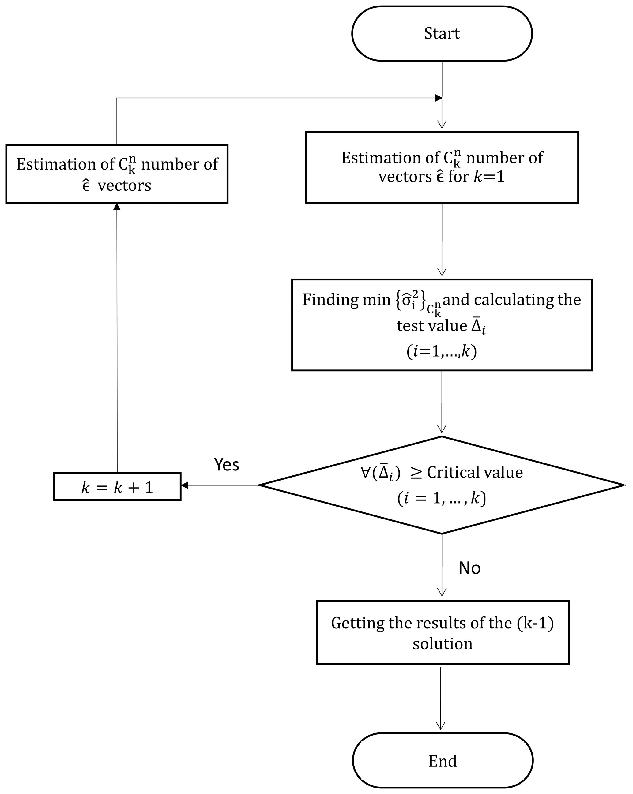
\begin{matrix} (35) & \begin{aligned} A_{C_{3}^{n}}^{3, 1} & = [\begin{array}{lllllllllll} 1 & 0 & 0 & 0 & - 1 & 0 & 0 & | & 1 & 0 & 0 \\ 1 & 0 & 0 & 0 & 0 & - 1 & 0 & | & 0 & 1 & 0 \\ 1 & - 1 & 0 & 0 & 0 & 0 & 0 & | & 0 & 0 & 1 \\ 0 & - 1 & 0 & 0 & 0 & 1 & 0 & | & 0 & 0 & 0 \\ ⋮ & ⋮ & ⋮ & ⋮ & ⋮ & ⋮ & ⋮ & | & ⋮ & ⋮ & ⋮ \\ 0 & 0 & 0 & 0 & - 1 & 0 & 1 & | & 0 & 0 & 0 \end{array}], \\ A_{C_{3}^{n}}^{3, 2} = [\begin{array}{lllllllllll} 1 & 0 & 0 & 0 & - 1 & 0 & 0 & | & 1 & 0 & 0 \\ 1 & 0 & 0 & 0 & 0 & - 1 & 0 & | & 0 & 1 & 0 \\ 1 & - 1 & 0 & 0 & 0 & 0 & 0 & | & 0 & 0 & 0 \\ 0 & - 1 & 0 & 0 & 0 & 1 & 0 & | & 0 & 0 & 1 \\ ⋮ & ⋮ & ⋮ & ⋮ & ⋮ & ⋮ & ⋮ & | & ⋮ & ⋮ & ⋮ \\ 0 & 0 & 0 & 0 & - 1 & 0 & 1 & | & 0 & 0 & 0 \end{array}] . \end{aligned} \end{matrix}

If all three values of unknowns exceed the critical value, they are flagged as outliers. This process is repeated for four or more combinations until all the combinations of potentially burdened observations have been considered. The $\hat{ϵ}$ vector of the observations corresponding to the minimum-variance value calculated for each combination step is compared with the critical value. If at least one of the relevant unknowns of the observations does not exceed the critical value, the H₀ hypothesis is accepted and the observations flagged in the previous step (i.e., the latest rejected H₀) are approved as outliers. The flowchart of the FSME (forward search of model error) model is presented in Fig. 1.

Table 1MSR of models (small outliers).

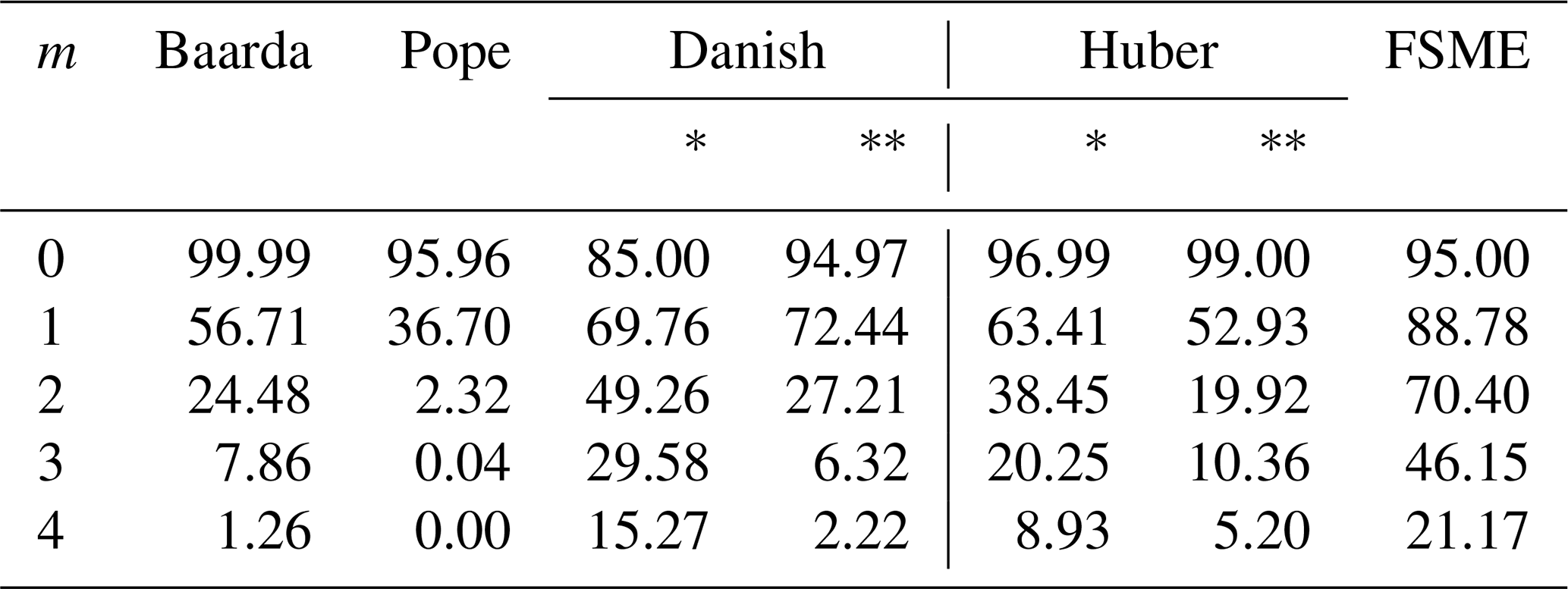
Two cases which the variance is known and unknown were considered for robust methods as follows: ^* The a priori variance is known. Here, the c was taken to be 1.5, where c=1.5σ₀ and σ₀=1. When the residual from the robust techniques exceeded the 3σ₀ threshold value, it was regarded as an outlier. In the case where the a priori variance is known, it can be seen in Table 1 that the MSRs of the robust methods are higher by 0.001 than the Baarda test with α considered. Pope's test had a lower MSR than Baarda's test. However, the MSRs of the FSME are higher than the robust methods in both cases where the a priori variance is known and unknown. $^{* *}$ The a priori variance is unknown. The standard deviation from the first iteration (LSE) was obtained for robust methods. So the c was taken from 1.5m₀. α was chosen as 0.05 for the Pope's test, which had a lower MSR than Baarda's. Except for the Danish* method, all other models identified an excellent observation as an outlier with a risk ranging from 0.01 % to 5 % if there was no outlier in the observations. The a posteriori variance negatively impacted the robust method's results, and the outlier's spoilt variance significantly contributed to the false detection. The a priori variance significantly affects how reliable the procedures are.

Download Print Version | Download XLSX

Table 2Local MSRs (small outliers).

Download Print Version | Download XLSX

4 Leveling network

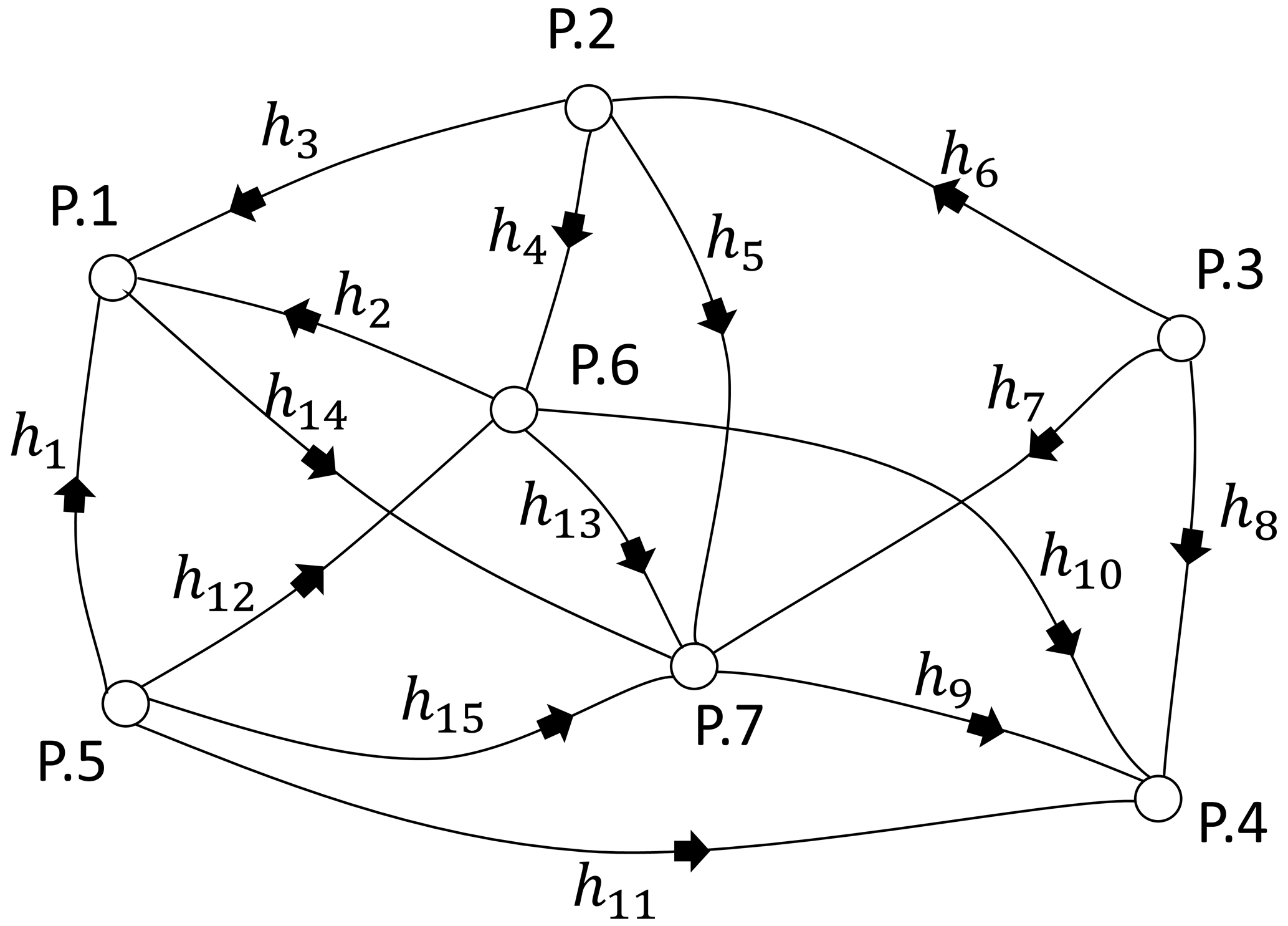
In statistics, there are different indicators to measure the reliability of tests and estimators. Hekimoglu and Koch (2000) showed that a finite-sample breakdown point determined the global reliability of an estimator and a test procedure. Using the power function of the global test, a capacity in deformation networks is explored as suggested by Niemeier (1985). Also, it has been shown that the MSR results of the two testing procedures (χ² and F test) are identical to their respective test powers known beforehand (Aydin, 2012). MSR depends on the number of outliers, the magnitude of an outlier, the number of unknowns, the number of observations, and the type of outliers. Since it considers these different cases, MSR is more reliable, whereas the power of the test is the same for all disparate conditions. Also, Erdogan et al. (2019) has proven that the MSR is the empirical estimation of the power of the test in outlier detection. In this study, therefore, MSR is used to specify the ability of the conventional, robust, and proposed models. By this purpose three different leveling networks have been simulated. The random errors ε_i for i=1…n were generated using a normal distribution N(0, σ²) with a mean of zero and a variance of σ². Also, the good and contaminated observations were acquired by simulation technique as described in detail by Hekimoglu and Erenoglu (2007). Since the outliers are produced through simulation, it is easy to determine whether an observation is burdened before analyzing. The method is deemed successful if the observation recognized as an outlier matches the really burdened observation. The process is considered unsuccessful if it fails. When the simulated observation is chosen randomly, the successful rate indicates that the global MSR and the local MSR can be computed for each particular observation in the leveling network for 10 000 samples. The same samples were subjected to conventional, robust, and proposed methods to compare their MSRs with different scenarios. This study simulated outliers randomly chosen from small- and large-magnitudes outliers (variously described as gross and influential outliers) for three leveling networks. An influential outlier is a situation that, either independently or when combined with other biased observations, adversely affects the outcomes of an analysis. Even a single influential outlier may ruin the estimation parameters. A leveling network used for the simulation has 7 points and 15 observations as seen in Fig. 2. The precision is considered to be $σ_{i}^{2} = σ_{0} / \sqrt{S}$ , where S is the length of the leveling line in kilometers and σ₀=1 mm ${\sqrt{1 km}}^{- 1}$ . MSRs for 10 000 samples were calculated for each method when there were different magnitudes and different numbers of outliers in the network. The small and large outliers were generated in the intervals of [3–6σ] and [6–12σ], respectively.

https://gmd.copernicus.org/articles/17/2187/2024/gmd-17-2187-2024-f02

Figure 2Leveling network.

Download

https://gmd.copernicus.org/articles/17/2187/2024/gmd-17-2187-2024-f03

Figure 3Leveling networks 2a and 2b with low redundancy.

Download

As Table 1 shows, even if the number of outliers changes, the MSRs of the proposed method increase significantly compared to the conventional and robust methods. In cases where there is no outlier (e.g., m=0), the results in which the H₀ hypothesis is rejected are also seen in Table 1. The proposed method generated type-II errors at the rate of 5 %, where the significance level was at 0.05.

Additionally, the a posteriori variance is easily influenced by outliers in the data set, which harms the abilities of methods that use the a posteriori variance. The a posteriori variance from the LSE is typically utilized as a threshold value instead of the a priori variance if the a priori variance is unknown. Therefore, the MSRs of the robust techniques of the former case are higher than the latter. As a result of these findings, only the case where the variance is known, which is less affected by an outlier, is taken into account in the results shown in the tables (Tables 2–8) to compare with the FSME hereafter.

5 Results

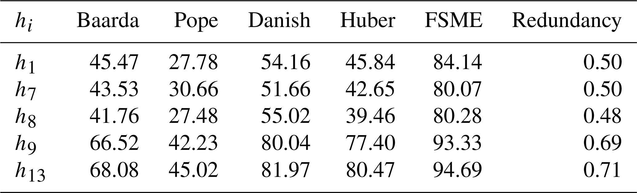
Extensive experiments have been done to compare the proposed method with robust methods, such as the Danish and Huber methods, besides the conventional outlier detection procedures (i.e., Baarda and Pope). The redundancies are an important indicator to recognize the observations most vulnerable to bias (Durdag, 2022). The redundancy matrix is calculated from $R = H - E$ , where $H = A (A^{T} PA)^{- 1} A^{T} P$ is a hat matrix. The local MSRs have been calculated for the specific observations with the highest and lowest redundancy in the leveling network. Among the observations, those with the two largest redundancies are h₁₃ and h₉, and the three lowest are h₁, h₇, and h₈. As can be seen from the Table 4 below, MSRs increase as the redundancy does.

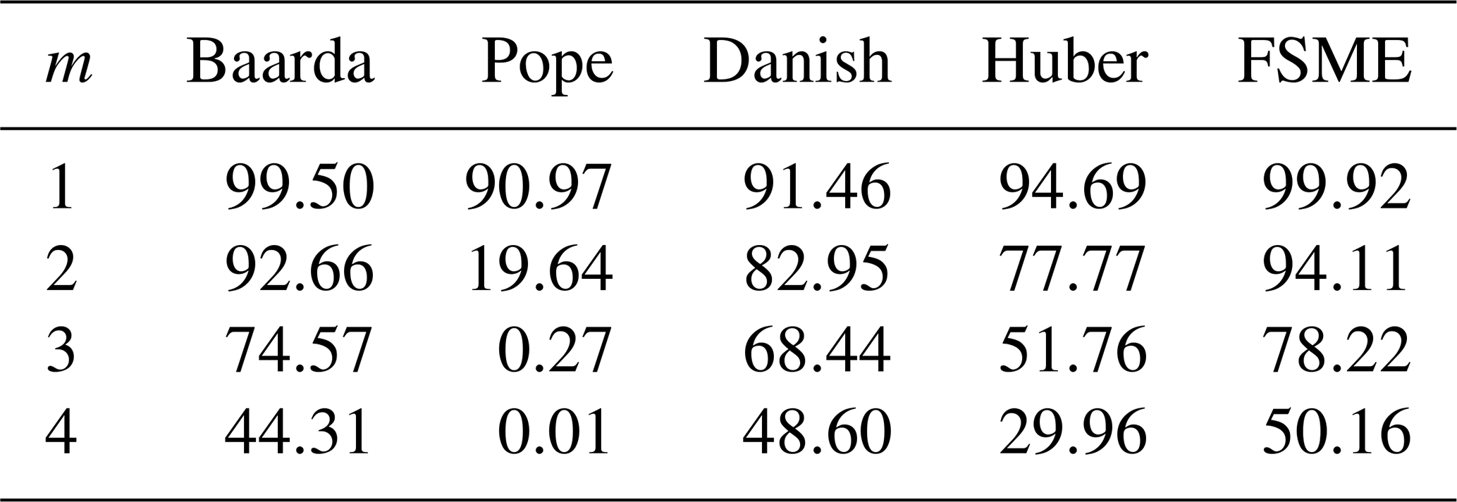
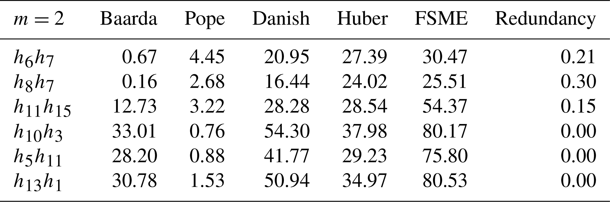
Table 3MSR of models (large outliers).

Download Print Version | Download XLSX

Table 4The effect of large and low partial redundancies on MSRs for a pair of observations.

Download Print Version | Download XLSX

Table 5MSRs for gross and influential outliers.

Download Print Version | Download XLSX

It is apparent from Table 2 that the highest MSRs for the biased observation h₁ amongst the conventional and robust methods are from the Danish method (54 %). In addition, the MSR of the proposed method is higher than the Danish one by 30 %. The highest MSR has been obtained by the FSME as 94 % for the observation with the highest redundancy h₁₃. As the redundancy gets smaller, the difference in MSR between the proposed method and other methods increases.

As shown in Table 3, the highest MSRs are obtained by the FSME in contrast with other techniques for different numbers of outliers. When Tables 1 and 3 are compared, the MSRs increase with an enlargement in the magnitude of outlier.

The smearing effect of the LSE, almost equivalent to its SC (sensitivity curve), behaves systematically as a function of the partial redundancy (Durdag, 2022). For this reason, the MSRs have been calculated for the pair of observations with the lowest and largest partial redundancy with small outliers in Table 4. The neighboring observations, especially the point that has three leveling lines, are some of the most vulnerable to bias (e.g., h₆h₇ and h₈h₇) in the leveling network (Fig. 2). The local MSRs are lower than the global MSRs, in the case m=2 in Table 1, for observations most vulnerable to bias with both the lowest and highest redundancies as shown in Table 4.

The results, as shown in Table 4, indicate that the MSRs of observation h₆h₇ with the highest partial redundancies increases compared to h₁₃h₁ with the lowest ones by almost 30 % for the Baarda and Danish models and 50 % for the FSME model.

It is apparent from Table 5 that Baarda and Danish are the two most successful methods against gross and influential outliers among classical and robust methods. In the case of small outliers with gross or influential outliers, the robustness of the models has been tested. Different types of outliers have been generated to evaluate the MSRs of the models for various scenarios as follows: (I) gross outlier (50σ), (II) influential outliers (1000σ), (III) a small outlier and a gross outlier, (IV) a small outlier and an influential outlier, (V) two small outliers and a gross outlier, and (VI) two small outliers and an influential outlier.

Table 6MSRs for small outliers with gross or influential outliers.

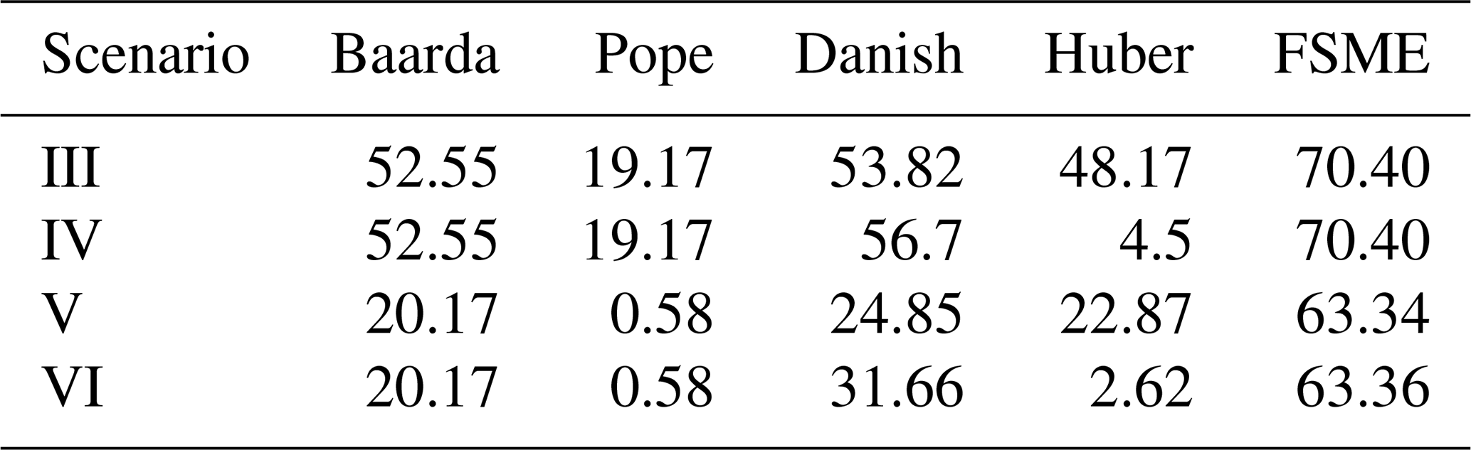
Download Print Version | Download XLSX

Comparing Table 5 with Table 6, it is observable how MSRs of these two methods were affected in case of one or two small outliers. If a small outlier occurs, the MSRs drop dramatically by about 40 %. The MSRs drop to 20 % with two small outliers in the network. Furthermore, this loss is around 35 %–40 % for the proposed method. The FSME, however, stands out as the model with an MSR of 60 %–70 % in scenarios involving small outliers.

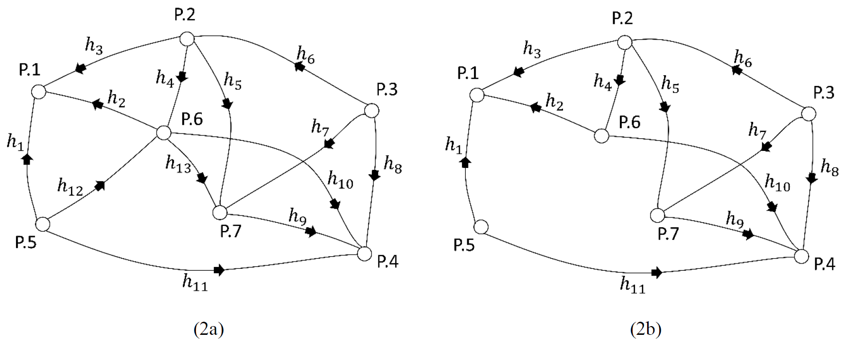
When the redundancies of the observations decrease in the leveling network, difficulties arise in determining the outliers due to the swamping and masking effects. Two different leveling networks are considered to obtain the MSR of the methods in such cases. In the first of these, the MSR of the models has been compared by excluding an observation of the network. As seen in Table 7, the MSR decreased by 30 % in all models when m=2, compared with the case m=1. Although the number of small outliers changes, the highest MSRs have been obtained by the FSME for the leveling network 2a. The network is further weakened, so only two lines of the corner point P.5 remain in the leveling network 2b.

Table 7MSR of models (small outliers) for leveling network 2a.

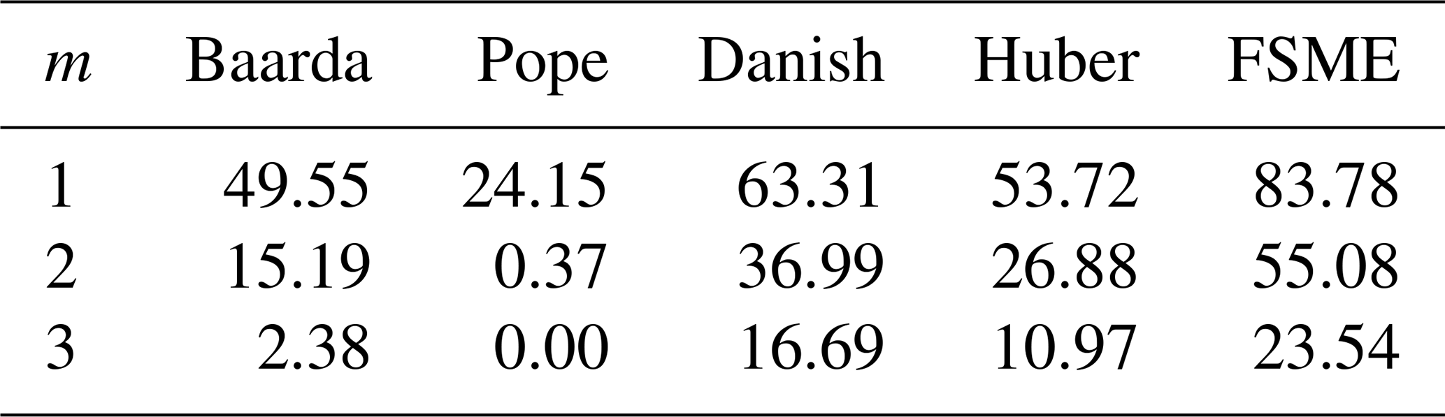
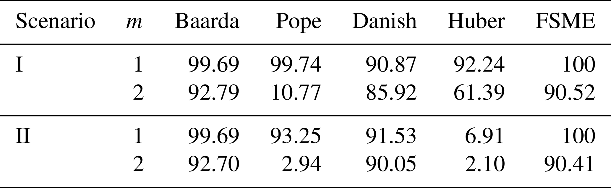
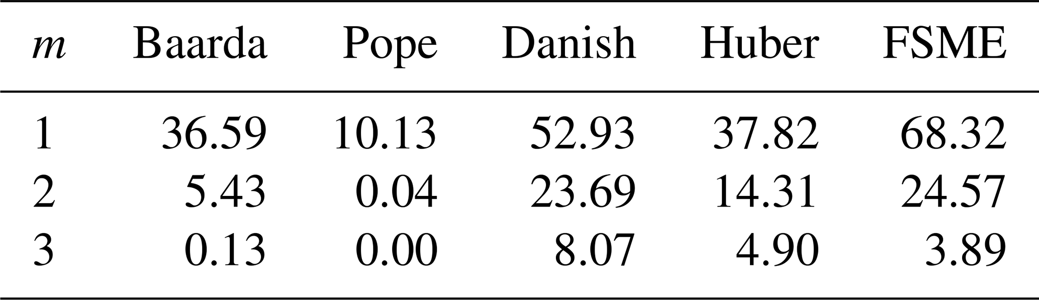
Download Print Version | Download XLSX

The results, as shown in Table 8, indicate that the FSME is the model with the highest MSR for m=1. When m>1 is compared with the case m=1 in Table 8, MSRs of the conventional and robust methods show a more dramatic decrease than the FSME model. Comparing the estimated results for the networks 2a and 2b reveals an approximately 15 % drop in MSR values when m=1. MSRs decrease as the controllability of the observations in the network decreases.

Table 8MSR of models (small outliers) for leveling network 2b.

Download Print Version | Download XLSX

6 Conclusion

Since geodetic observations are utilized in studies requiring high accuracy for determining deformations, detecting and identifying outliers become increasingly critical. Researchers commonly favor conventional and robust methods based on the additive bias model. However, this study contributes to our understanding by advancing the modeling of outliers as an additional unknown parameter within the Gauss–Markov model. The aim of this study was to evaluate the suitability of the FSME method within geodetic networks. To achieve this objective, the FSME method was applied to a leveling network. The design of the FSME method is based on identifying the minimum variance from all possible combinations that assume observations as model errors in the Gauss–Markov model. Although only a leveling network has been simulated, the functional and stochastic models of the FSME methods can be applied to all type of geodetic networks. This model yields more reliable results by preventing the swamping and masking effect. The MSRs of the suggested method were obtained for various outliers in three different leveling networks. The results of this investigation show that the FSME is a more efficient model than the robust and conventional methods. Specifically, the proposed method enhanced the MSR by almost 40 %–45 % compared to the Baarda and Danish (with the variance unknown case) methods for multiple outliers (i.e., 1<m<4). Moreover, in scenarios where specific observations were absent at corner points in leveling network 1, the proposed method exhibited 20 %–30 % greater success than alternative methods. Despite the proposed model demonstrating a higher MSR than other methods, the FSME method may encounter numerous combinations depending on the presence of observations and outliers. To address this challenge, particularly in real-world applications, the MSS (maximum subsample method) proposed by Neitzel (2004) and Ebeling (2014) offers a promising approach to reduce the number of combinations in outlier detection procedures. As demonstrated by Ebeling in deformation monitoring, MSS holds potential as a valuable tool to enhance the applicability of the proposed method, particularly within extensive geodetic networks.

Code and data availability

The current code version is available from the project website: https://doi.org/10.5281/zenodo.10417506 (Durdağ, 2023) under the MIT license. The exact version of the model used to produce the results used in this paper is archived on Zenodo (https://doi.org/10.5281/zenodo.10417506, Durdağ, 2023), as are input data and scripts to run the model and produce the plots for all the simulations presented in this paper.

Competing interests

The author has declared that there are no competing interests.

Disclaimer

Publisher’s note: Copernicus Publications remains neutral with regard to jurisdictional claims made in the text, published maps, institutional affiliations, or any other geographical representation in this paper. While Copernicus Publications makes every effort to include appropriate place names, the final responsibility lies with the authors.

Acknowledgements

The author expresses sincere gratitude to the anonymous referees and Xinyue Yang for their valuable comments and suggestions, which have significantly enhanced the quality of this paper.

Review statement

This paper was edited by Yongze Song and reviewed by two anonymous referees.

References

Aydin, C.: Power of global test in deformation analysis, J. Surv. Eng., 138, 51–56, https://doi.org/10.1061/(ASCE)SU.1943-5428.0000064, 2012.

Baarda, W.: A testing procedure for use in geodetic networks. Publications on Geodesy, 2 = 5, Netherlands Geodetic Commission, Delft, the Netherlands, ISBN 90 6132 209 X, 1968.

Batilović, M., Sušić, Z., Kanović, Ž., Marković, M. Z., Vasić, D., and Bulatović, V.: Increasing efficiency of the robust deformation analysis methods using genetic algorithm and generalised particle swarm optimisation, Surv. Rev., 53, 193–205, https://doi.org/10.1080/00396265.2019.1706294, 2021.

Duchnowski, R.: Sensitivity of robust estimators applied in strategy for testing stability of reference points. EIF approach, Geodesy and Cartography, 60, 123–134, https://doi.org/10.2478/v10277-012-0011-z, 2011.

Durdağ, U. M.: Godesist/OutlierDetectionForGeodeticLevelingNetwork: Initial Release (0.1.0), Zenodo [code and data set], https://doi.org/10.5281/zenodo.10417506, 2023.

Durdag, U. M., Hekimoglu, S., and Erdogan, B.: What is the relation between smearing effect of least squares estimation and its influence function? Surv. Rev., 54, 320–331, https://doi.org/10.1080/00396265.2021.1939590, 2022.

Ebeling, A.: Ground-Based Deformation Monitoring. PhD Thesis, University of Calgary, Department of Geomatics Engineering, Calgary, https://doi.org/10.11575/PRISM/26325, 2014.

Erdogan, B.: An outlier detection method in geodetic networks based on the original observations, Bol. Ciênc. Geod., 20, 578–589, https://doi.org/10.1590/S1982-21702014000300033, 2014.

Erdogan, B., Hekimoglu, S., Durdag, U. M., and Ocalan, T.: Empirical estimation of the power of test in outlier detection problem, Studia Geophys. et Geod., 63, 55–70, https://doi.org/10.1007/s11200-018-1144-9, 2019.

Gao, Y., Krakiwsky, E. J., and Czompo, J.: Robust testing procedure for detection of multiple blunders, J. Surv. Eng., 118, 11–23, https://doi.org/10.1061/(ASCE)0733-9453(1992)118:1(11), 1992.

Hekimoglu, S.: Reliabilities of χ²-and F Tests in Gauss-Markov Model, J. Surv. Eng., 125, 109–135, https://doi.org/10.1061/(ASCE)0733-9453(1999)125:3(109), 1999.

Hekimoglu, S.: Increasing reliability of the test for outliers whose magnitude is small, Surv. Rev., 38, 274–285, https://doi.org/10.1179/sre.2005.38.298.274, 2005.

Hekimoglu, S. and Erenoglu, R. C.: Effect of heteroscedasticity and heterogeneousness on outlier detection for geodetic networks, J. Geod., 81, 137–148, https://doi.org/10.1007/s00190-006-0095-z, 2007.

Hekimoglu, S. and Koch, K. R.: How can reliability of the test for outliers be measured?, Allgemeine Vermessungsnachrichten, 107, 247–254, 2000.

Hekimoglu, S., Erdogan, B., and Butterworth, S.: Increasing the efficacy of the conventional deformation analysis methods: alternative strategy, J. Surv. Eng., 136, 53–62, https://doi.org/10.1061/(ASCE)SU.1943-5428.0000018, 2010.

Hekimoglu, S., Erdogan, B., Soycan, M., and Durdag, U. M.: Univariate approach for detecting outliers in geodetic networks, J. Surv. Eng., 140, 04014006, https://doi.org/10.1061/(ASCE)SU.1943-5428.0000123, 2014.

Hekimoglu, S., Erdogan, B., and Erenoglu, R. C.: A new outlier detection method considering outliers as model errors, Exp Techniques, 39, 57–68, https://doi.org/10.1111/j.1747-1567.2012.00876.x, 2015.

Huber, P. J.: Robust Estimation of a Location Parameter, Ann. Math. Stat., 35, 73–101, http://www.jstor.org/stable/2238020 (last access: 12 March 2024), 1964.

Huber, P. J.: Robust Statistics, John Wiley and Sons, New York, USA, 312 pp., ISBN 9780471418054, 1981.

Koch, K. R.: Parameter estimation and hypothesis testing in linear models, Springer, New York, USA, 334 pp., ISBN 978-3-540-65257-1, 1999.

Lehmann, R.: 3σ-rule for outlier detection from the viewpoint of geodetic adjustment, J. Surv. Eng., 139, 157–165, https://doi.org/10.1061/(ASCE)SU.1943-5428.0000112, 2013.

Maronna, R. A., Martin, R. D., Yohai, V. J., and Salibián-Barrera, M.: Robust statistics: theory and methods (with R), Wiley, Chichester, UK, 430 pp., ISBN 9781119214687, 2019.

Neitzel, F.: Identifizierung konsistenter Datengruppen am Beispiel der Kongruenzuntersuchung geodätischer Netze, PhD thesis, Deutsche Geodätische Kommission, Reihe C, Nr. 565, München, ISSN 0065 5325, ISBN 3 7696 5004 2, https://www.researchgate.net/profile/Frank-Neitzel/publication/35226424 (last access: 14 March 2024), 2004.

Niemeier, W.: Anlage von Überwachungsnetzen. Geodaetische Netze in Landes- und Ingenieurvermessung II., edited by: Pelzer, H., Verlag Konrad Wittwer, Stuttgart, Germany, 527–558, ISBN 3879191298, LCCN 80491066, 1985 (in German).

Nowel, K.: Specification of deformation congruence models using combinatorial iterative DIA testing procedure, J. Geod., 94, 118, https://doi.org/10.1007/s00190-020-01446-9, 2020.

Pope, A. J.: The statistics of residuals and the detection of outliers. NOAA Technical Rep. NOS 65 NGS 1, U.S. Dept. of Commerce, Rockville, Maryland, USA, 98 pp., https://repository.library.noaa.gov/view/noaa/30811 (last access: 13 March 2024), 1976.

Teunissen, P. J.: Testing theory; an introduction, VSSD Leeghwaterstraat 42, 2628 CA Delft, the Netherlands, 147 pp., ISBN 978-9040719752, 2006.

Wang, J., Zhao, J., Liu, Z., and Kang, Z.: Location and estimation of multiple outliers in weighted total least squares, Measurement, 181, 109591, https://doi.org/10.1016/j.measurement.2021.109591, 2021.

Zienkiewicz, M. H. and Dąbrowski, P. S.: Matrix Strengthening the Identification of Observations with Split Functional Models in the Squared M_split(q) Estimation Process, Measurement, 217, 112950, https://doi.org/10.1016/j.measurement.2023.112950, 2023.

Articles

Short summary

This study introduces a novel approach to outlier detection in geodetic networks, challenging conventional and robust methods. By treating outliers as unknown parameters within the Gauss–Markov model and exploring numerous outlier combinations, this approach prioritizes minimal variance and eliminates iteration dependencies. The mean success rate (MSR) comparisons highlight its effectiveness, improving the MSR by 40–45 % for multiple outliers.