the Creative Commons Attribution 4.0 License.
the Creative Commons Attribution 4.0 License.
 | 26 Feb 2024
Carbon isotopes in the marine biogeochemistry model FESOM2.1-REcoM3
Christoph Völker
Özgür Gürses
Judith Hauck
Peter Köhler
In this paper we describe the implementation of the carbon isotopes 13C and 14C (radiocarbon) into the marine biogeochemistry model REcoM3. The implementation is tested in long-term equilibrium simulations where REcoM3 is coupled with the ocean general circulation model FESOM2.1, applying a low-resolution configuration and idealized climate forcing. Focusing on the carbon-isotopic composition of dissolved inorganic carbon (δ13CDIC and Δ14CDIC), our model results are largely consistent with reconstructions for the pre-anthropogenic period. Our simulations also exhibit discrepancies, e.g. in upwelling regions and the interior of the North Pacific. Some of these differences are due to the limitations of our ocean circulation model setup, which results in a rather shallow meridional overturning circulation. We additionally study the accuracy of two simplified modelling approaches for dissolved inorganic 14C, which are faster (15 % and about a factor of five, respectively) than the complete consideration of the marine radiocarbon cycle. The accuracy of both simplified approaches is better than 5 %, which should be sufficient for most studies of Δ14CDIC.
- Article
(21139 KB) - Full-text XML
- BibTeX
- EndNote


Carbon isotopes are powerful tools for tracing present and past biogeochemical cycles and water masses. The stable isotope carbon-13 (13C) can be used to study the anthropogenic perturbation of the global carbon cycle owing to the combustion of isotopically depleted fossil fuels via the so-called 13C Suess effect (e.g. Keeling, 1979; Quay et al., 1992; Köhler, 2016; Graven et al., 2021). Carbon-13 may also help to decipher the exchange between atmospheric, marine, and terrestrial carbon reservoirs in the past, for example, during the last glacial cycle (Köhler et al., 2006; Ciais et al., 2012; Broecker and McGee, 2013; Jeltsch-Thömmes et al., 2019; Menking et al., 2022). Furthermore, 13C is a proxy for oceanic nutrients and can be employed to infer past marine biological productivity, export production, and water mass distributions assuming that calcareous tests of foraminifera are faithful recorders of dissolved inorganic 13C (e.g. Broecker and Peng, 1982; Lynch-Stieglitz et al., 2007; Hesse et al., 2011; Schmittner et al., 2017). The radioactive isotope carbon-14 (radiocarbon, 14C) is the most important geochemical chronometer for dating organic matter and for assessing ocean ventilation rates and pathways over the last 55 000 years (Heaton et al., 2021; Rafter et al., 2022; Skinner and Bard, 2022, Skinner et al., 2023). In addition, the penetration of bomb-produced 14C into the oceans has provided a benchmark for ocean circulation models (Matsumoto et al., 2004). Although the potential of carbon isotopes has been known for a long time, ocean general circulation models have only recently been equipped with carbon isotopes and applied in Earth system modelling studies (e.g. Tschumi et al., 2011; Holden et al., 2013; Schmittner et al., 2013; Jahn et al., 2015; Menviel et al., 2015; Buchanan et al., 2019; Jeltsch-Thömmes et al., 2019; Dentith et al., 2020; Tjiputra et al., 2020; Claret et al., 2021; Liu et al., 2021; Morée et al., 2021).
Here, we describe the implementation of both carbon isotopes 13C and 14C into the marine biogeochemistry model REcoM3, which is part of the AWI Earth System Model. The technical details are described in Sect. 2 and simulations in Sect. 3. Isotope results are presented in terms of δ13C and Δ14C, which express the relative deviations of observed (13R) and (14R) ratios with respect to specific standard values 13Rstd and 14Rstd, where
and (following Stuiver and Pollach, 1977)
Section 4 concludes with a brief summary.
2.1 Short overview of REcoM3
The Regulated Ecosystem Model, version 3 (REcoM3) is described in detail by Gürses et al. (2023). Here, we only give a brief summary of the common model features and describe the differences from the configuration that we use in this study. REcoM considers the marine biogeochemical cycles of carbon, nitrogen, silicon, iron, and oxygen. The ecosystem component of REcoM includes nutrients, two phytoplankton functional types (distinguishing between small phytoplankton and diatoms), one zooplankton functional type, one detritus type, and dissolved organic matter. Different from most other marine biogeochemistry models, REcoM does not rely on a fixed internal stoichiometry of phytoplankton. Instead, the composition of organic soft tissue is regulated (i.e. calculated) in response to light, temperature, and nutrient supply, which enables stoichiometric shifts between the present and past to be assessed. The model includes a sediment layer in which sinking detritus (consisting of particulate organic matter, calcite, and opal) is fully remineralized and where solutes are returned to the bottom water layer within days so that there is no accumulation of sedimentary matter. Alternatively, REcoM3 can be run with the comprehensive sediment model MEDUSA2 (Munhoven, 2021), which is described in another paper (Ye et al., 2023). Apart from the implementation of carbon isotopes, the main difference from the standard REcoM3 configuration by Gürses et al. (2023) is that REcoM3 considers two zooplankton and two detritus groups instead of one, which would require inclusion of six additional carbon-isotopic tracers at the expense of model speed. We refer to the configuration presented here as REcoM3p as an initial set-up for paleo studies. To simulate biogeochemical tracer circulation, REcoM3 needs a transport model. Here, we utilize the ocean general circulation model FESOM2.1, which is an update of FESOM2.0 (Danilov et al., 2017). The coupling of FESOM2.1 with REcoM3 is also described by Gürses et al. (2023), where all biogeochemical model equations except for carbon isotopes can be found.
2.2 Implementation of carbon isotopes
Carbon-13 and 14C are implemented as additional passive tracers, tripling the number of carbon-containing tracers in REcoM from 8 to 24. The model considers carbon isotopes for dissolved inorganic and organic carbon, small phytoplankton, diatoms, zooplankton, detritus, and calcite. As the abundances of 13C and 14C are small (13Rstd≈0.0113, Assonov et al., 2020, and ; Orr et al., 2017), we approximate total C with 12C and neglect 13C and 14C in the kinetic calculations of the carbonate system. For the same reason, and to ensure numerical stability in the other model calculations involving 13C and 14C, the model considers scaled concentrations 13C and 14C, which have the same magnitude as 12C, following Jahn et al. (2015). As a consequence, 13C′ and 14C′ have to be rescaled when compared with observed concentrations. However, as the scaling factors cancel out when 13C′ and 14C′ are converted to δ13C and Δ14C, Eqs. (1)–(3) can be directly evaluated with scaled concentration ratios and .
We consider isotopic fractionation during air–sea gas exchange, dissolution of CO2 in seawater, and photosynthesis by phytoplankton. In addition, the model accounts for radioactive decay and, optionally, cosmogenic production of 14C. The details are explained in the following subsections.
2.3 Carbon-13
2.3.1 Air-sea exchange
The isotopic fractionation during uptake and dissolution of 13CO2 is calculated according to Zhang et al. (1995), similar to the biogeochemical protocol of the CMIP6 Ocean Model Intercomparison Project (OMIP-BGC protocol, Orr et al., 2017). That is, the air–sea exchange flux 13F is proportional to the difference between the saturation and in situ concentrations of aqueous 13CO2:
where kw is the CO2 gas transfer velocity (calculated according to Wanninkhof, 2014, additionally considering sea-ice cover), and [13CO]sat and [13CO] are the saturation and in situ concentrations of aqueous 13CO2. 13Ratm and 13RDIC are the concentration ratios of atmospheric CO2 and dissolved inorganic carbon (DIC). Isotopic fractionation factors α denote kinetic fractionation during CO2 gas transfer (13αk), equilibrium fractionation during gas dissolution (13αaq−g), and equilibrium fractionation between DIC and gaseous CO2 (13αDIC−g). Numerical values were taken from Zhang et al. (1995), who measured kinetic and equilibrium fractionation of 13C in acidified freshwater. For kinetic fractionation we employ a constant value of 13αk=0.99912, which is the average between 5 °C (13αk=0.99919) and 21 °C (13αk=0.99905). Equilibrium fractionation between aqueous and atmospheric 13CO2 is expressed as
where T (°C) is the temperature of surface water. The numerical values of 13αk and 13αaq−g were determined for fresh water. To account for enhanced 13C fractionation in seawater associated with hydration reactions, Eq. (4) includes a correction factor of −0.0002 following Zhang et al. (1995), which is not considered in the OMIP-BGC protocol. Fractionation between DIC and gaseous CO2 is calculated as
where fCO3= [CO] DIC is the carbonate fraction of DIC.
2.3.2 Biogenic fractionation
Photosynthesis of phytoplankton leads to isotopic depletion of particulate organic carbon (POC), which is expressed following Freeman and Hayes (1992):
where [13CPOC] and [12CPOC] are the isotopic POC concentrations in phytoplankton, 13RPOC is the corresponding isotopic ratio, 13Raq is the concentration ratio of aqueous CO2, and 13αp is the isotopic fractionation factor associated with photosynthesis. Various experimental and modelling studies have determined 13αp for certain phytoplankton species (Laws et al., 1995; Rau et al., 1996; Bidigare et al., 1997; Laws et al., 1997; Rau et al., 1997; Popp et al., 1998; Keller and Morel, 1999). However, it is uncertain to what extent these studies are globally representative and can be transferred into a single global modelling framework (see also the review by Brandenburg et al., 2022). Therefore, we pursue a less sophisticated but robust approach to calculating 13αp, which does not rely on species-specific assumptions and has been inferred from a global dataset of 525 δ13CPOC field measurements spanning the period 1962–2010 CE (Young et al., 2013):
where [CO] is in µmol L−1. As no distinction is made between different phytoplankton species in Eq. (8), the carbon-isotopic composition of small phytoplankton and diatoms in our model is the same. Similar to other models (e.g. Schmittner et al., 2013; Menviel et al., 2015; Buchanan et al., 2019; Tjiputra et al., 2020; Liu et al., 2021), we do not consider carbon-isotopic fractionation during the formation and dissolution of biogenic calcite because the effect is small and varies between species (α∼0.999–1.003 according to Ziveri et al., 2003).
2.4 Radiocarbon
Radiocarbon is subject to radioactive decay, cosmogenic production, and isotopic fractionation. The radioactive decay (applying a half-life of 5700 years, Audi et al., 2003; Bé and Chechev, 2012; Kutschera, 2013) is balanced in the model by cosmogenic 14C production fluxes or, alternatively, by prescribed atmospheric 14CO2 concentrations corresponding to atmospheric Δ14C values.
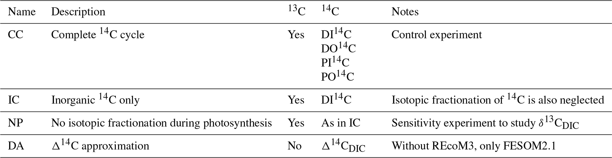
Fractionation factors are calculated analogously to 13α, with (e.g. Craig, 1954; see also the discussion by Fahrni et al., 2017). The slow equilibration of DI14C in the deep ocean requires spinup simulations of several thousands of years, which may be computationally too expensive for high-resolution simulations. Therefore, we have implemented 14C in various ways that differ in their level of complexity and computational efficiency. The first implementation (“CC”) considers the complete 14C cycle parallel to 13C. The second implementation (“IC”) disregards the isotopic fractionation of 14C and radioactive decay of organic matter. In turn, DI14C and DIC have identical sources and sinks, except for atmospheric CO2 and radioactive decay. This “inorganic” 14C approach is an approximation that is conceptually similar, but not identical, to the “abiotic” 14C modelling approach described in the OMIP biogeochemical protocol (Orr et al., 2017). In our IC approach, DIC and DI14C include biological sources and sinks. This does not apply to the OMIP-abiotic approach, which also considers alkalinity in a simplified way. In Sect. 3.3 we scrutinize the accuracy of the IC approximation. The third approach takes advantage of the fact that marine Δ14C values of DIC (Δ14CDIC) are primarily governed by transport and radioactive decay (Fiadeiro, 1982; see also Mouchet, 2013). This implies that Δ14CDIC can be implemented into ocean general circulation models as a single prognostic tracer without a full carbon cycle model (see Toggweiler et al., 1989, and numerous other studies later on). We evaluate this Δ14C approximation (“DA”) in an additional simulation and compare it with REcoM approaches CC and IC in Sect. 3.3 too.
A list of the various model experiments and their key features can be found in Table 1.
3.1 Simulated ocean climatology
FESOM employs unstructured meshes with variable horizontal resolution. The default mesh of FESOM2.1-REcoM3 has about 127 000 horizontal surface nodes (Gürses et al., 2023). Here, our model resolution is radically reduced, considering 3140 surface nodes corresponding to a median horizontal resolution of 260 km (the so-called pi-mesh, see Fig. A1 in Appendix A). This configuration requires fewer computational resources and allows simulations over the time scale of marine carbon isotope equilibration to be performed (i.e. over several thousand years) within a few weeks. Vertical resolution is 47 layers using z* coordinates with non-linear free surface (for further details see Scholz et al., 2019).
In a first step we run FESOM without REcoM over 1000 years to spinup the overturning circulation and thermohaline fields. FESOM was initialized with seasonal winter temperatures and salinities by Steele et al. (2001), and driven with annually repeated atmospheric fields using Corrected Normal Year Forcing Version 2.0 (Large and Yeager, 2009; for an overview see also Griffies et al., 2012). As FESOM2.1 had originally been adjusted for higher resolution and different forcing, we retuned the model in our setup by reducing the maximum Gent–McWilliams thickness diffusivity from 2000 m2 s−1 originally to 1000 m2 s−1. After 1000 simulated years there was no significant drift of thermohaline fields and the meridional overturning circulation (MOC) had stabilized, REcoM3p was turned on, and both models were run over an additional 5000 years. At this moment, temperature and salinity drifted by about 10−6 K per year and 10−6 PSU per year in the global average, and the major biogeochemical tracer inventories drifted by less than 10−3 % per year (less than 10−3 ‰ per year regarding DI13C and DI14C). REcoM3p was initialized with gridded concentration fields of total alkalinity, DIC, and nitrate from version 2 of the Global Ocean Data Analysis Project (GLODAPv2, Key et al., 2015; Lauvset et al., 2016), oxygen from the World Ocean Atlas 2018 (WOA18, Garcia et al., 2019), silicate from Ocean Atlas 2013 (WOA13, Garcia et al., 2014), and dissolved iron according to Aumont et al. (2003) and Tagliabue et al. (2012). Dissolved inorganic 13C and 14C were initialized with DIC, assuming initial fractionation values of δ13CDIC=0 ‰ and Δ14C ‰ respectively. In the sediment layer all initial concentrations were close to zero. REcoM3p was forced with constant atmospheric CO2 concentrations ([12CO2]atm=284.3 ppmv; [13CO2]atm and [14CO2]atm corresponding to δ13C ‰ and Δ14Catm=0 ‰ respectively, following Orr et al., 2017), and with climatological mean monthly fluxes of aeolian iron deposition (Albani et al., 2014). The CO2 concentration forcing implies that carbon-isotopic mass is only conserved in the atmosphere-ocean system when the marine isotopic inventories have reached a corresponding steady state. In our simulations this is the case after a few thousand years (see further below).
As discussed in the following, our low-resolution test setup sufficiently captures the basic thermohaline circulation structures obtained with FESOM2.0 in higher-resolution simulations (Scholz et al., 2019, 2022; compare their Figs. 14, 15, and 17 with our Figs. A2–A4 in Appendix A). Compared with observations, our simulations exhibit a warm bias for thermocline and intermediate water as well as for North Atlantic Deep Water (NADW; see Fig. A2 in Appendix A). The most notable exception is the region of the North Atlantic Gulf stream, which is not properly resolved, and where upper ocean temperatures are considerably underestimated. The temperature biases covary with salinity biases. That is, simulated salinities are also higher than observations where simulated temperatures are high, and salinities are too low where simulated temperatures tend to be low (Fig. A3). In the Atlantic, FESOM arrives at a MOC of about 16 Sv (1 Sv = 1×10⁶ m3 s−1, Fig. A4), which is at the lower bound of observations, whereas the simulated overturning cell is too shallow compared with observational estimates (see Buckley and Marshall, 2016, and further references therein). For the purposes of this study, our simulations also reasonably reflect the observed large-scale pattern of DIC (Key et al., 2015; Lauvset et al., 2016). That is, low concentrations are found at upper levels of the subtropical oceans and in the freshly ventilated interior of the North Atlantic, whereas DIC concentrations progressively increase in the South Atlantic and in the deep North Pacific (Fig. A5).
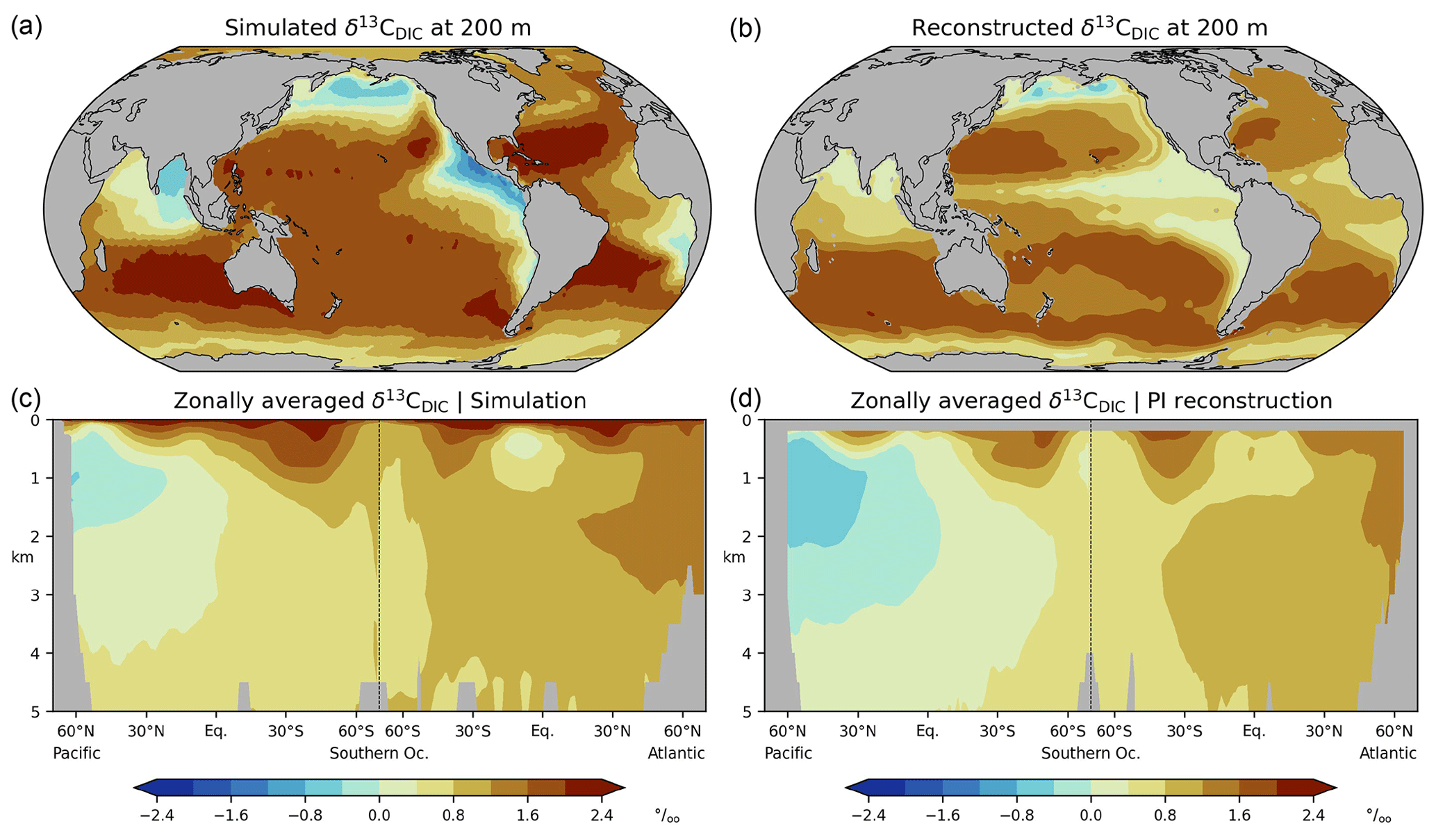
Figure 1Preindustrial δ13C of DIC, (a, c) this study (simulation CC), (b, d) reconstruction (Eide et al., 2017b). (a, b) values at 200 m depth, (c, d) zonal-mean values in the Atlantic and Pacific. Map projection here and in other figures is area preserving (Equal Earth projection, Šavrič et al., 2019).
3.2 Carbon-13
We now focus on the carbon-isotopic composition of DIC near the sea surface and along zonal-mean sections through the Atlantic and Pacific. Regarding δ13CDIC, we compare our model results with the gridded preindustrial (PI) δ13CDIC climatology by Eide et al. (2017b). Their reconstruction does not consider the upper 200 m to exclude the 13C Suess effect. For the sake of completeness, we briefly note that at the sea surface our δ13CDIC results are largely in line with ungridded preindustrial values determined by Kwon et al. (2022; shown in Fig. A6).
In wide areas, our simulated near-surface δ13CDIC values at 200 m are within the range 1 ‰ to 2 ‰ (Fig. 1a). Higher δ13CDIC values are simulated in the subtropical oceans, particularly in the Atlantic, southeast Pacific, and southern Indian Ocean. Isotopic depletion of up to ‰ is found in the eastern equatorial Pacific, the subpolar North Pacific, the Bay of Bengal, and in the Angola Basin. Although our simulation captures the reconstructed spatial pattern (shown in Fig. 1b), the simulated range of δ13CDIC variations is larger than in the reconstruction, that is, the model results are too high in the lower latitudes and too low in the abovementioned depletion regions (Fig. 2a).
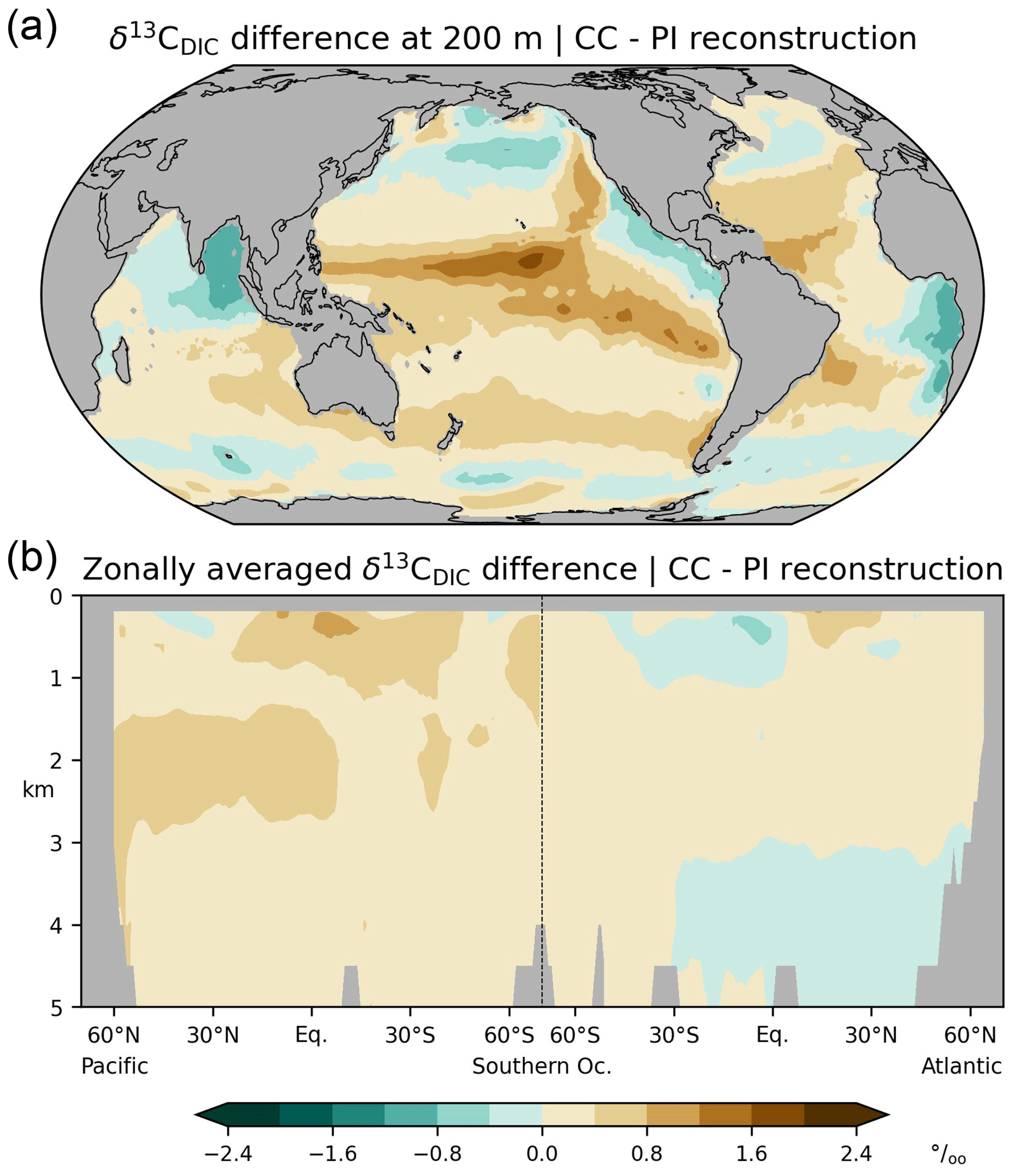
Figure 2Differences between simulated (this study; CC) and reconstructed (Eide et al., 2017b; PI) δ13C of DIC for the preindustrial period; (a) at a depth of 200 m, (b) zonal-mean values in the Atlantic and Pacific.
Considering the interior of the Atlantic Ocean, our simulation yields higher δ13CDIC in the North Atlantic than in the South Atlantic, and small vertical δ13CDIC gradients in the high latitudes of both hemispheres (Fig. 1c). In the Pacific, our simulation displays a reversed meridional δ13CDIC gradient with the strongest isotopic depletion at intermediate depths in the North Pacific. Our results are roughly in line with the reconstruction by Eide et al. (2017b, see Fig. 1d) but overestimate δ13CDIC in the upper Pacific at low latitudes as well as in the North Pacific at a depth of between 1.5 and 3 km (Fig. 2b). Similar inaccuracies are seen in other models (Tagliabue an Bopp, 2008; Schmittner et al., 2013; Jahn et al., 2015; Buchanan et al., 2019; Jeltsch-Thömmes et al., 2019; Dentith et al., 2020; Tjiputra et al., 2020; Liu et al., 2021).
The differences between simulated and reconstructed δ13CDIC (the δ13CDIC bias for short) can be attributed to various factors. First, the reconstructed δ13CDIC values may be too low in the upper ocean if the 13C Suess effect is not completely removed from the observations. In fact, Eide et al. (2017a) presume that they may have underestimated the 13C Suess effect at a depth of 200 m by about 0.1 ‰ to 0.2 ‰, which has been corroborated in recent modelling studies (Liu et al., 2021; Kwon et al., 2022). This reconstruction bias partly corresponds to the apparent simulation bias at a depth of 200 m, where our model results are 0.2 ‰ higher on global average than the reconstructed results.
To some extent, the δ13CDIC bias can be further attributed by decomposing δ13CDIC into biologic and thermodynamic sources:
where δ13CBIO specifies the imprint of isotopic fractionation, respiration, and remineralization of organic matter in the absence of air–sea exchange. Following Broecker and Maier-Reimer (1992), δ13CBIO is frequently determined from the covariation of δ13CDIC with marine phosphate (PO). We adopt this approach, employing revised parameter values by Eide et al. (2017b) and tentatively replacing PO with dissolved inorganic nitrogen (DIN) divided by 16 because PO is not considered by REcoM3p:
where PO and DIN are in µmol kg−1. Equation (10) does not distinguish between preformed and remineralized nutrient concentrations and cannot be used for further separation of δ13CBIO into preformed and remineralized components. The thermodynamic component δ13CAS describes the effects of air–sea exchange and ocean circulation and is the residual of observed δ13CDIC and reconstructed δ13CBIO.
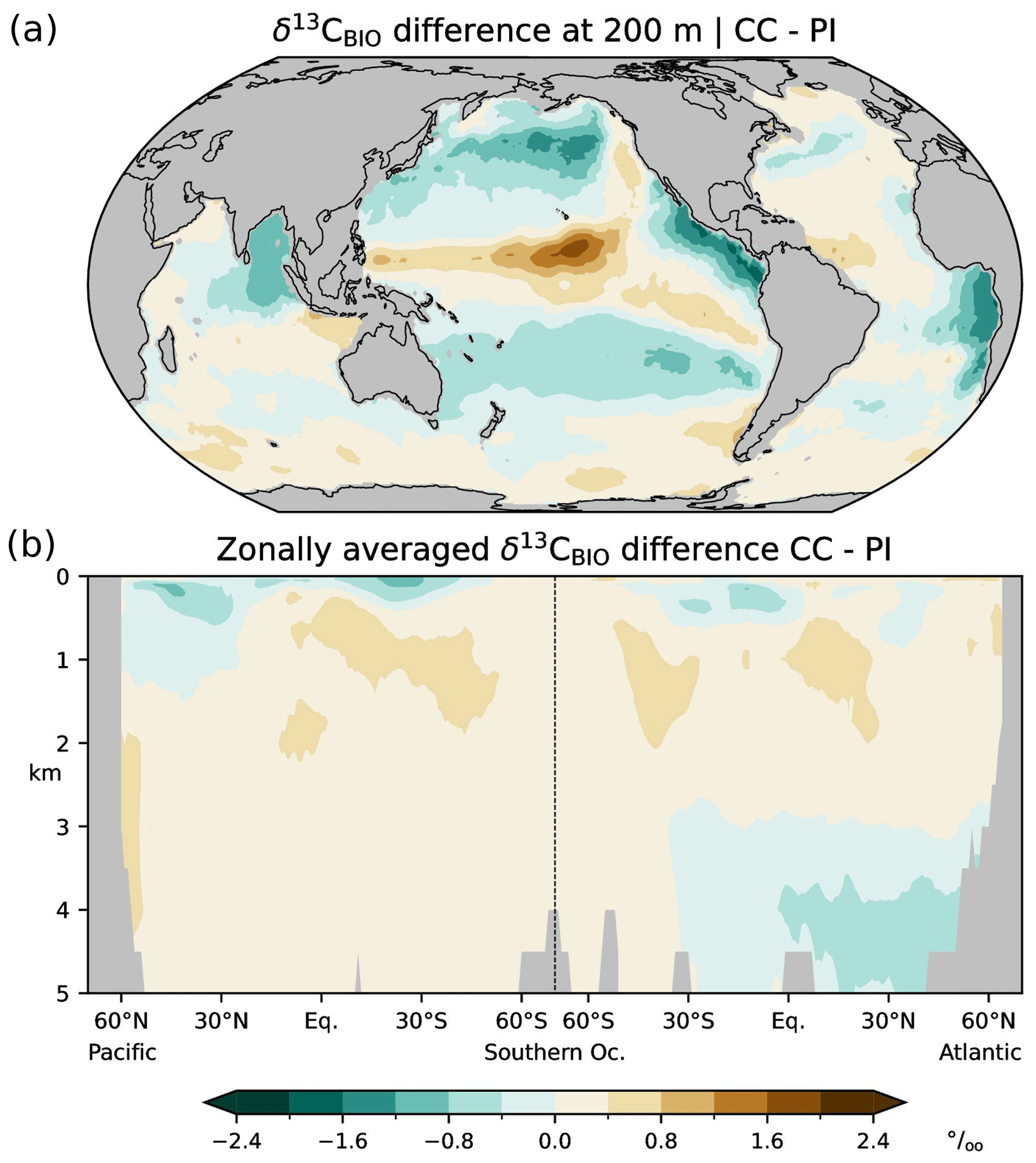
Figure 3Differences between simulated (this study; CC) and estimated (Eide et al., 2017b; PI) δ13CBIO (the biological component of δ13CDIC in the absence of air–sea exchange) during the preindustrial period; (a) at a depth of 200 m, (b) zonal-mean values in the Atlantic and Pacific.
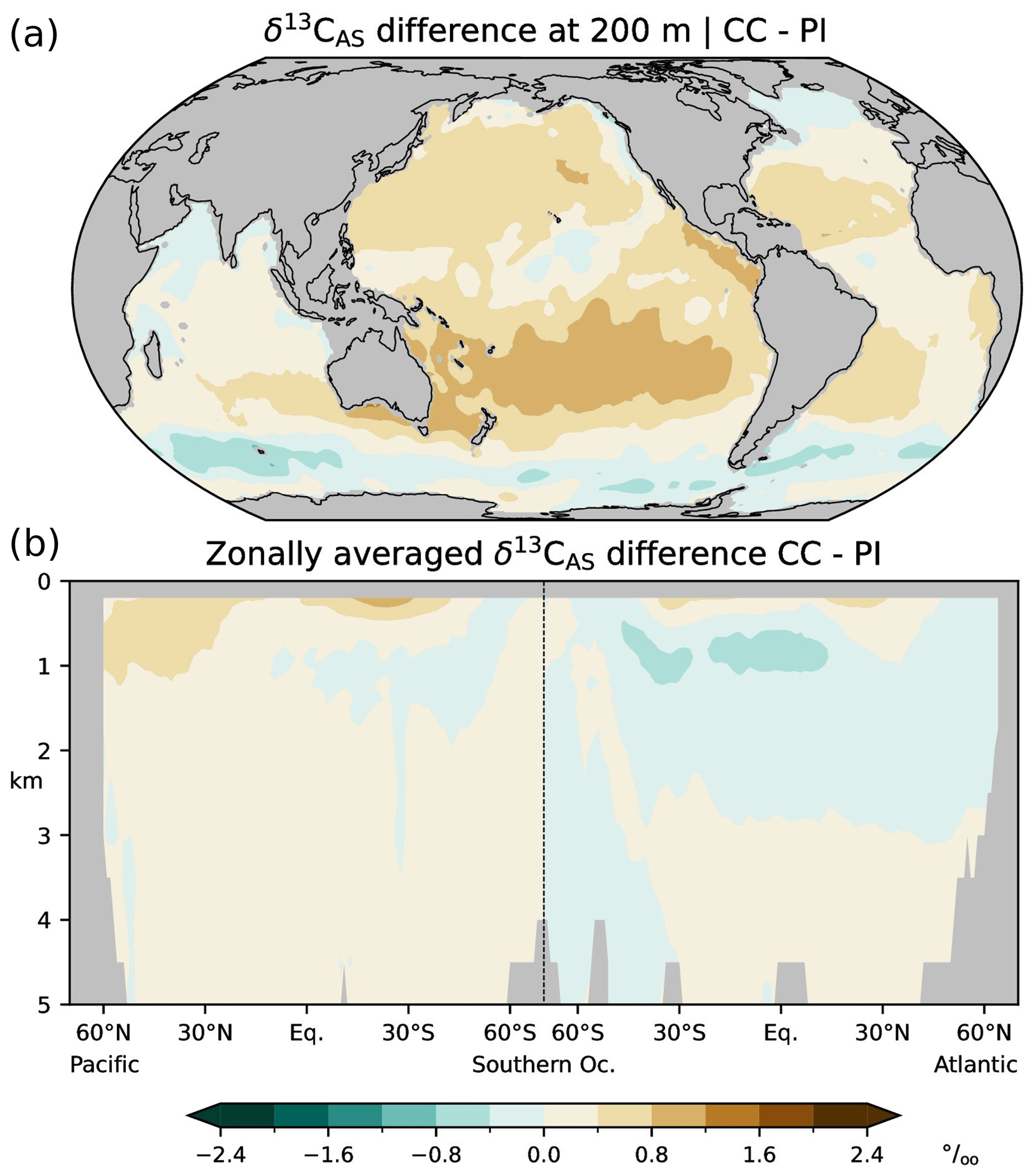
Figure 4Differences between simulated (this study; CC) and estimated (Eide et al., 2017b; PI) δ13CAS=δ13CDIC−δ13CBIO during the preindustrial period; (a) at a depth of 200 m, (b) zonal-mean values in the Atlantic and Pacific.
In the following we validate simulated δ13CBIO and δ13CAS with the corresponding values reconstructed by Eide et al. (2017b), and we compare the δ13CDIC bias with the differences between the simulated and reconstructed δ13CDIC components, i.e. the δ13CBIO bias and δ13CAS bias. Simulation CC overestimates δ13CBIO in wide areas, except for subtropical and upwelling regions at 200 m and the North Atlantic below 3 km (Fig. 3). The simulation also overestimates δ13CAS in the thermocline but underestimates δ13CAS in the interior of the North Atlantic above about 3 km (Fig. 4). Comparing the biases of δ13CDIC, δ13CBIO and δ13CAS, it appears that the δ13CDIC bias corresponds to the δ13CBIO bias in the low latitudes, upwelling regions, and the interior of the Atlantic (see Figs. 2 and 3). This points to model deficiencies in describing the sinking and regeneration of 13C-depleted organic carbon. On the other hand, the δ13CDIC bias corresponds to the δ13CAS bias in the upper thermocline of the open oceans in the Southern Hemisphere (shown in Fig. 4). Although our results may generally suffer from the coarse model resolution and simplified climate forcing, the specific reasons for this correspondence are not obvious. As a residual term δ13CAS may also reflect effects of biological 13C cycling, which are not captured by Eq. (10). For example, δ13CBIO is estimated for constant isotopic fractionation of marine organic matter of −19 ‰ whereas δ13CPOC varies by about 10 ‰ according to field data (Verwega et al., 2021; see also Fig. 6a).
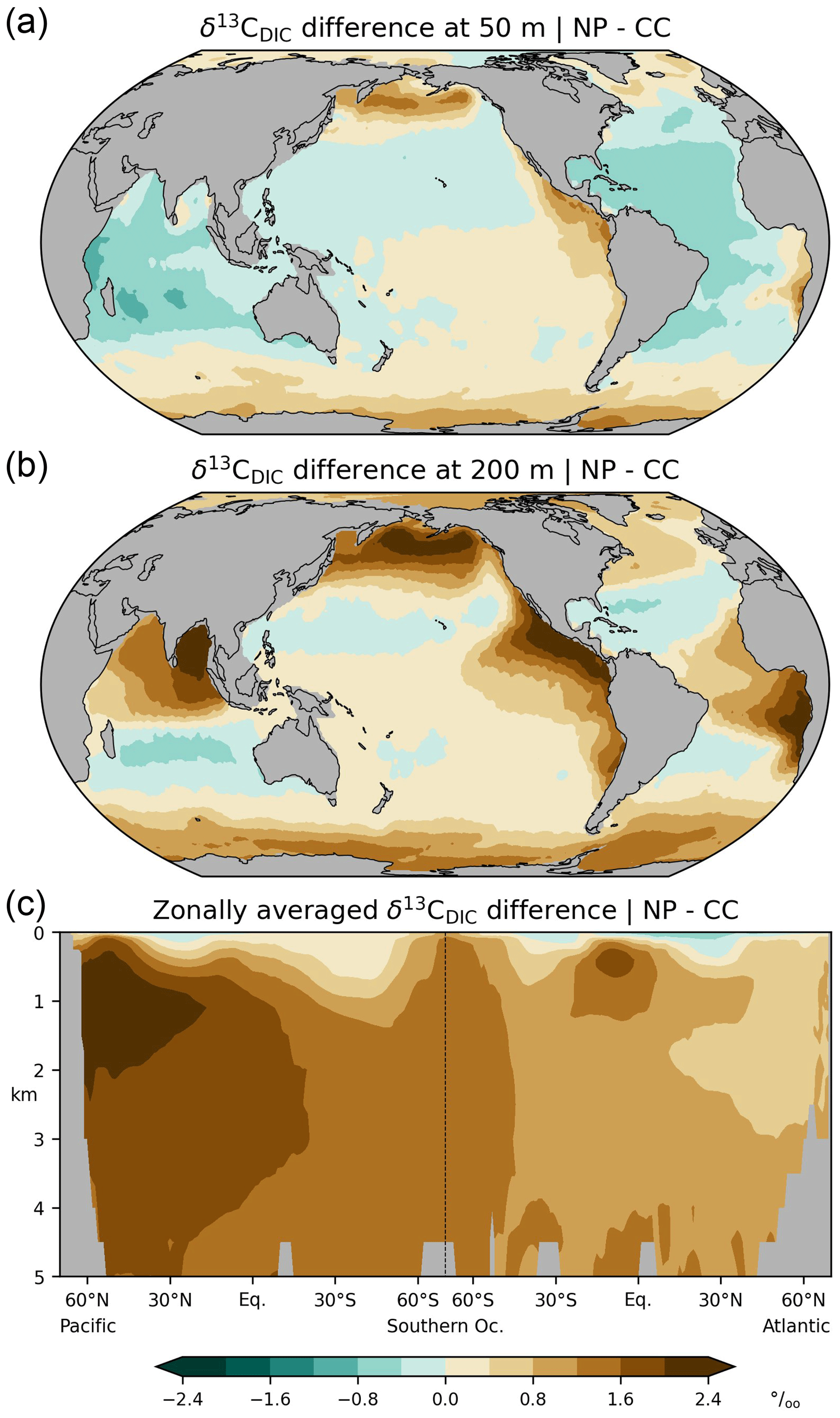
Figure 5Changes in preindustrial δ13C of DIC if isotopic fractionation during photosynthesis is disabled (sensitivity experiment NP versus simulation CC), (a) at a depth of 50 m, (b) at a depth of 200 m, (c) zonal-mean values in the Atlantic and Pacific.
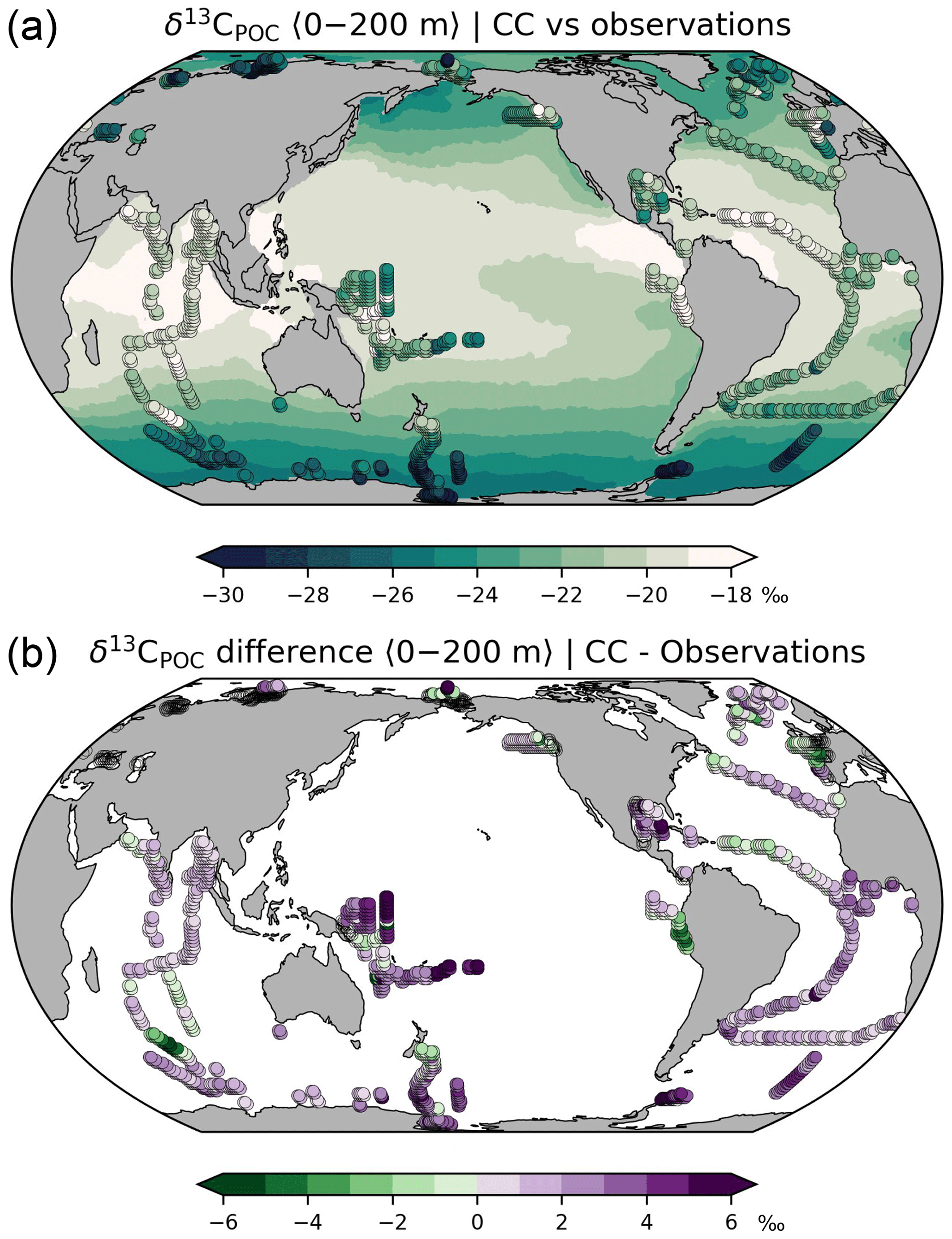
Figure 6(a) δ13C of POC averaged over the upper 200 m. Shaded areas: simulation results (this study; simulation CC), dots: bulk matter observations for the period 1964–2015 (compilation by Verwega et al., 2021; see further references therein). (b) Differences between simulated and observed δ13C of POC.
Therefore, we explore the sensitivity of δ13CDIC to photosynthetic fractionation in an additional experiment (“NP”) in which biogenic fractionation is disabled (i.e. 13αp=1 in Eq. 8). Compared with the default simulation, δ13CDIC|NP decreases by up to 1 ‰ in the pelagic euphotic zone whereas δ13CDIC|NP increases in the disphotic zone below, which is particularly the case in highly productive regions (Fig. 5a, b). In the aphotic interior of the ocean δ13CDIC|NP progressively increases from the North Atlantic towards the North Pacific by up to 2.4 ‰ (Fig. 5c). These findings are in line with similar sensitivity studies (Schmittner et al., 2013; Dentith et al., 2020) as well as with simulations comparing different parametrizations for 13αp (Jahn et al., 2015; Buchanan et al., 2019; Dentith et al., 2020; Liu et al., 2021).
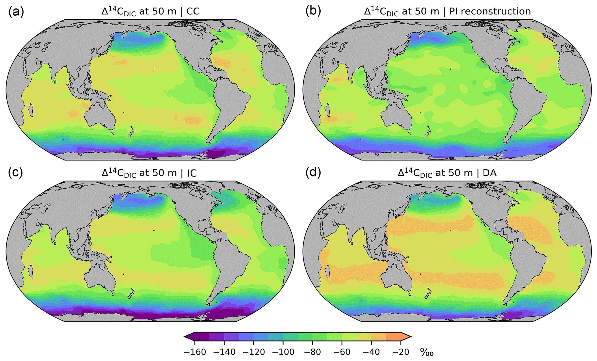
Figure 7Preindustrial Δ14C of DIC at a depth of 50 m, (a) simulation CC considering the complete marine 14C cycle, (b) reconstruction (Key et al., 2004), (c) simulation IC applying the inorganic 14C approximation, (d) simulation DA applying the Δ14C approach. See the main text for further explanations.
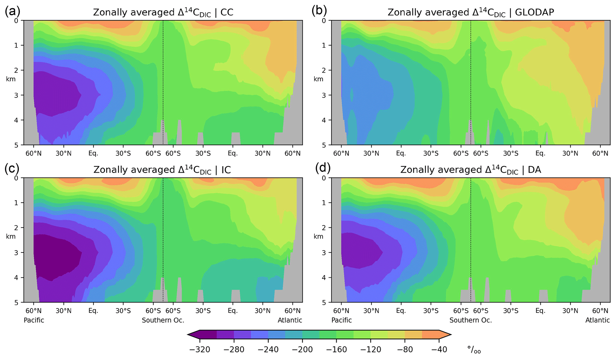
Figure 8Preindustrial Δ14C of DIC in the Atlantic and Pacific. (a) Simulation CC, (b) reconstruction (Key et al., 2004), (c) simulation IC, (d) simulation DA. See the main text for further simulation explanations. Note the different colour scale ranges in Figs. 7 and 8.
Our default simulation with enabled photosynthetic fractionation yields δ13CPOC values between −18 ‰ and −25 ‰ whereas observations from the last decades range from −15 ‰ to −35 ‰ (Verwega et al., 2021; Fig. 6a). The model overestimates δ13CPOC at most locations (Fig. 6b; global RMS difference is 2.6 ‰). According to the sensitivity experiment NP, the overestimation of δ13CPOC should result in overly enriched δ13CDIC in the twilight and dark zones of highly productive regions (Fig. 5b), whereas Fig. 2a indicates that the opposite is the case. However, this is only an apparent contradiction because the δ13CPOC observations are biased by the 13C Suess effect. Moreover, they exhibit a negative trend (by −3 ‰ between 1960 and 2010), which is about twice as high as the known 13C Suess effect on aqueous CO2 (Verwega et al., 2021). It has been presumed that this trend also reflects a shift in the composition of phytoplankton species (Lorrain et al., 2020; Verwega et al., 2021). Neither effect is considered in our simulation. A conclusive analysis would require transient simulations, including historical values of atmospheric 13CO2.
3.3 Radiocarbon
We consider Δ14CDIC and compare our model results with gridded fields of pre-bomb Δ14CDIC provided by the Global Ocean Data Analysis Project, version 1.1 (GLODAPv1.1, Key et al., 2004).
In the comprehensive radiocarbon cycle simulation (CC) Δ14CDIC|CC is within the range −40 ‰ to −140 ‰ (average value: −65 ‰) near the surface (at 50 m), with the highest values in the subtropical gyres and the lowest values in the Southern Ocean (Fig. 7a). In the interior of the Atlantic, Δ14CDIC|CC ranges between −70 ‰ and −170 ‰ and decreases from the surface to the bottom, with small vertical gradients in the high latitudes (Fig. 8a). This is superimposed by a southward decline of Δ14CDIC values. Conversely, Δ14CDIC decreases from south to north in the interior of the Pacific. Different from the northern North Atlantic, there is no evidence of deep-sea ventilation in the North Pacific, where our model arrives at minimum Δ14CDIC|CC values exceeding −290 ‰ (Fig. 8a). This depletion corresponds to a 14C age τ of about 2800 years with respect to the atmosphere (calculated as ).
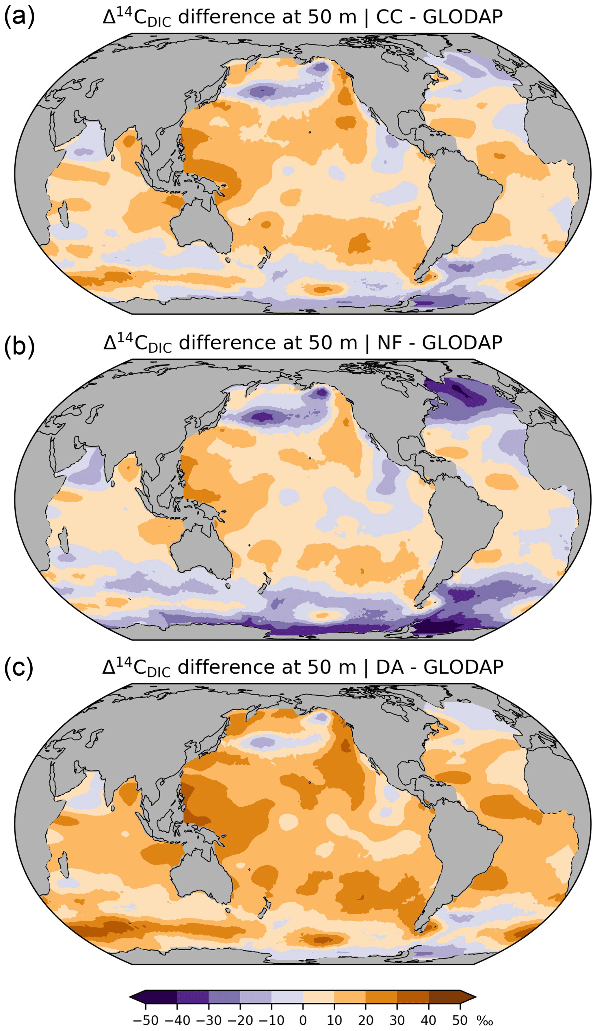
Figure 9Differences between simulated and reconstructed preindustrial Δ14C of DIC at a depth of 50 m, (a) simulation CC minus reconstruction (GLODAP; Key et al., 2004), (b) simulation IC minus reconstruction, (c) simulation DA minus reconstruction.
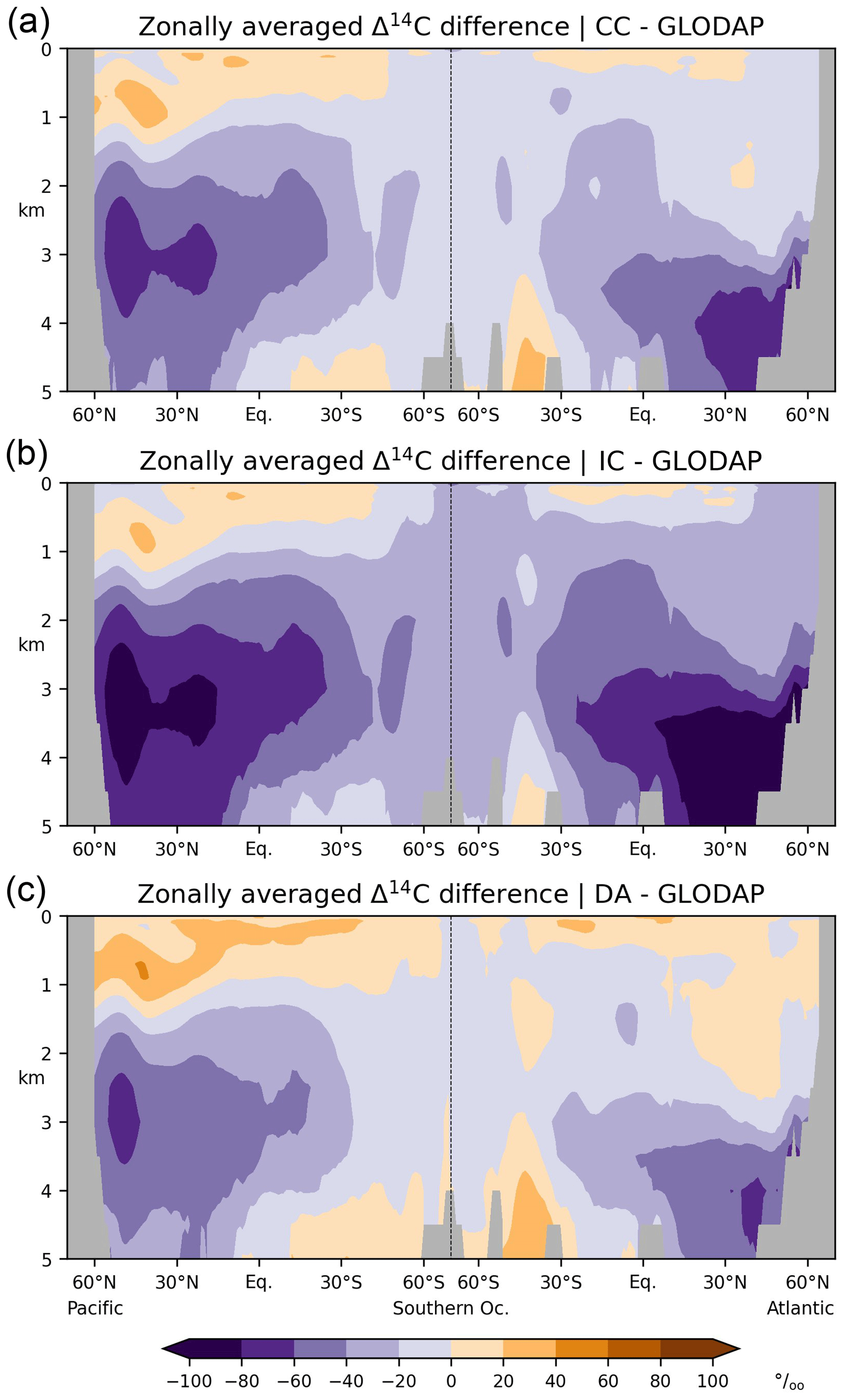
Figure 10Differences between simulated and reconstructed preindustrial Δ14C of DIC in the Atlantic and Pacific: zonal-mean values are shown, (a) simulation CC minus reconstruction (GLODAP; Key et al., 2004), (b) simulation IC minus reconstruction, (c) simulation DA minus reconstruction. Note the different colour scale ranges in Figs. 9 and 10.
Overall, simulation CC captures the large-scale distribution of pre-nuclear Δ14CDIC as reconstructed by GLODAPv1.1 (Figs. 7a, b, 8a, b). However, at a depth of 50 m the simulated Δ14CDIC is too high by 10 ‰–30 ‰ in the low- and mid-latitudes, and too low by about the same amount in the high latitudes (see Fig. 9a; according to GLODAP Δ14CDIC ranges from −50 ‰ to −170 ‰ with −71 ‰ on average). In the interior of the oceans, our model results are typically 20 ‰–60 ‰ too low (Fig. 10). The excessive depletion reaches −70 ‰ in the abyssal North Atlantic and in the North Pacific at 3 km depth (Fig. 10a). In the upper layers of the oceans, the GLODAPv1.1 data probably reflect the 14C Suess effect (Suess, 1955), which is not considered in our simulations. The excessive depletion in the deep sea indicates that the simulated MOC leads to overly shallow and weak ocean ventilation, which is particularly the case in the North Pacific. This effect is enhanced by the progressive radioactive decay of DI14C along its passage through the interior of the ocean.
Different from δ14CDIC, Δ14CDIC is corrected for isotopic fractionation. In practice (as well as in the comprehensive DI14C cycle modelling approach CC), the correction is made after the simultaneous determination of δ13CDIC and δ14CDIC. In the inorganic 14C (IC) modelling approach the fractionation of 14C is omitted beforehand, so that posterior corrections are not necessary. That is, δ14CDIC|IC equals Δ14CDIC|IC, which should equal Δ14CDIC|CC. As the IC approach also neglects the radioactive decay of organic carbon, it considers seven tracers less than the CC approach, which is accompanied by an increase in model speed (simulated years per day) of about 15 %.
At a depth of 50 m Δ14CDIC|IC ranges from −50 ‰ to −160 ‰ with an average value of 72 ‰ (Fig. 7c). Similar to experiment CC, the highest values of Δ14CDIC|IC are found in subtropical surface waters. The lowest surface water values of Δ14CDIC|IC are also found in the Southern Ocean. In the interior of the oceans, the isotopic depletion with respect to the atmosphere ranges from −90 ‰ in the North Atlantic to −310 ‰ in the North Pacific (Fig. 8c). Comparing IC with the GLODAPv1.1 reconstruction, we find that the enrichment of subtropical surface values is less pronounced in IC, whereas the depletion in the high latitudes increases (Fig. 9b). The latter is also the case in the interior of the oceans (Fig. 10b). Most notably, the outcomes of experiment IC are everywhere lower (by up to 30 ‰) than the results of simulation CC (Fig. 11a, c) which is explained as follows.
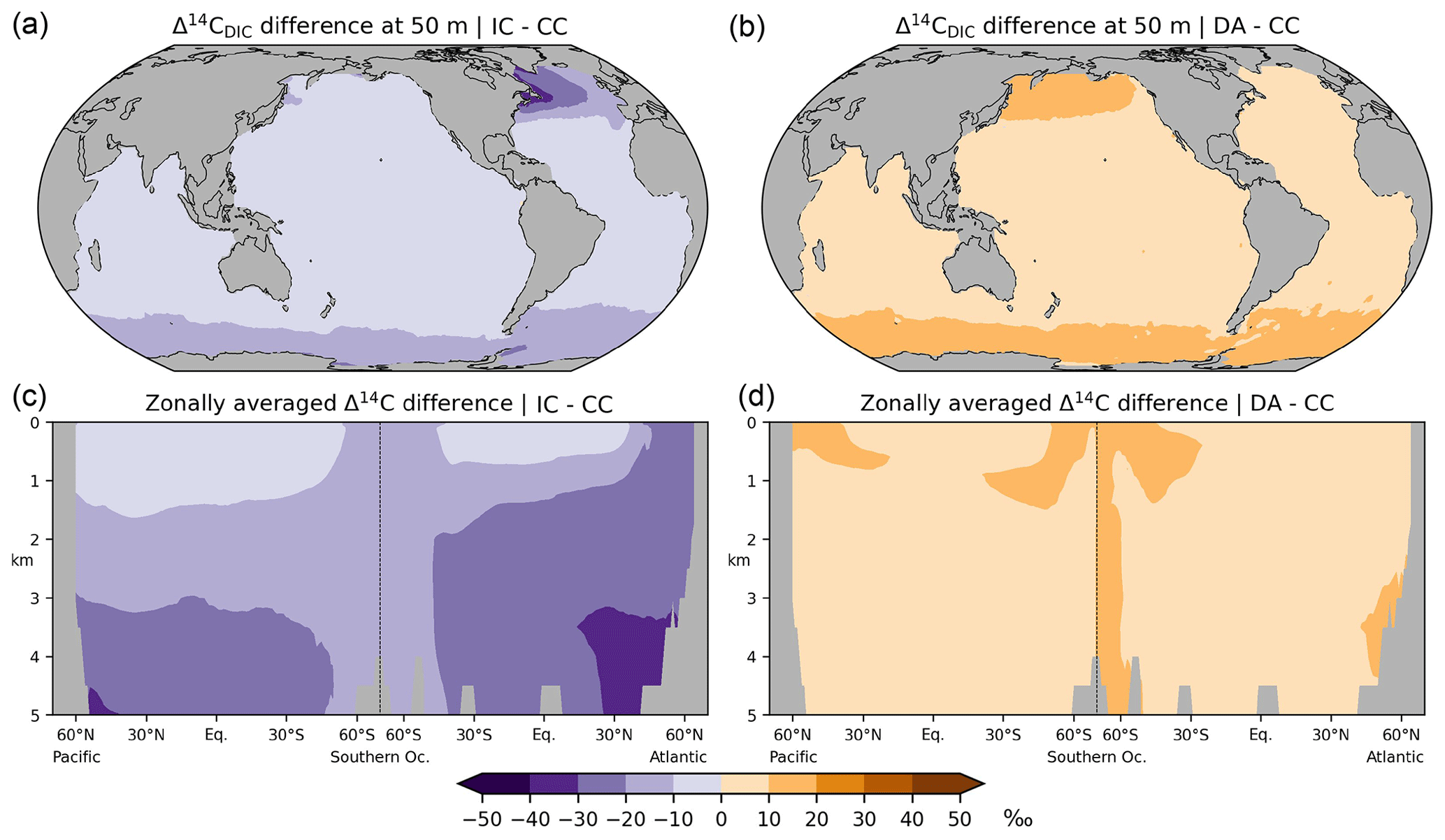
Figure 11Absolute differences in preindustrial Δ14CDIC between the various simulation approaches: results at a depth of 50 m (a, b) and in the Atlantic and Pacific (c, d) are shown. (a, c) Inorganic 14C (IC) modelling approach versus complete 14C cycle (CC), (b, d) Δ14C approximation (DA) versus simulation CC.
Analogous to sensitivity experiment NP, the IC approach disregards photosynthetic fractionation, which leads to lower DI14C concentrations in the euphotic zone than in simulation CC. In addition, the IC approach disregards the DI14C enrichment of the mixed layer associated with air–sea exchange. Furthermore, as the IC approach disregards the radioactive decay of phytoplankton, the loss of DI14C due to photosynthesis is overestimated in the mixed layer. Therefore, preformed DI14C is systematically lower than in simulation CC and becomes further depleted through radioactive decay in the deep sea. This bias is similar to the lower values of “abiotic” Δ14C than “biotic” Δ14C simulated by Frischknecht et al. (2022).
Instead of computing absolute concentrations of DIC, DI13C, and DI14C and converting them to Δ14CDIC a posteriori, the Δ14C approximation (DA) simulates as a single prognostic tracer that is considered abiotic and conservative except for its radioactive decay, and that is connected to the carbon cycle only through the timescale of 14CO2 air–sea exchange. This approach is about five times faster than the CC and IC approaches. The first results of the implementation of 14RDIC|DA into FESOM2 were shown by Lohmann et al. (2020) for the default FESOM mesh with 127 000 horizontal surface nodes. Here, we repeated the experiment, now using the low-resolution mesh of experiments CC and IC to be able to compare the results of all approaches directly. For the same reason, we discuss model results after 5000 simulated years but point out that experiment DA has been run over 17 000 years in total. The maximum drift of Δ14CDIC|DA between 5000 and 17 000 simulated years is about −3.5 ‰ in North Pacific Deep Water, which is much smaller than the Δ14CDIC differences between the various modelling approaches in this study after 5000 years shown below.
At at depth of 50 m Δ14CDIC|DA ranges from −40 ‰ to −130 ‰, with Δ14C ‰ on average (Fig. 7d). In intermediate and deep water Δ14CDIC|DA declines from −60 ‰ in the North Atlantic to −280 ‰ in the North Pacific (Fig. 8d). At upper levels, Δ14CDIC|DA is almost everywhere higher than Δ14CDIC according to GLODAPv1.1 (Figs. 9c, 10c). In the deep sea, Δ14CDIC|DA is still too low, but the depletion is less pronounced than in simulations CC and IC (Fig. 10c).
Experiment DA yields the highest Δ14CDIC values of all three modelling approaches (Fig. 11). The DA approach assumes that DIC concentrations are constant and homogeneous (for a rigorous treatise see Mouchet, 2013). Following Toggweiler et al. (1989), our calculation of 14CO2 air–sea exchange fluxes in simulation DA assumes a DIC concentration of 2000 mmol m−3 in the mixed layer, which is somewhat lower than that observed and simulated in most areas, most notably in the high latitudes (Fig. A5a, b). This leads to faster and hence higher 14C uptake in DA than in CC and IC because the 14CO2 invasion flux is inversely proportional to the DIC concentration in the mixed layer. The absolute Δ14CDIC differences between DA and CC are largely less than 10 ‰ (Fig. 11b, d). Moreover, the relative uncertainty of the DA approach with respect to the correct DI14C implementation (CC) is less than 5 % (Fig. 12) and actually smaller than the error of 10 % originally estimated by Fiadeiro (1982).
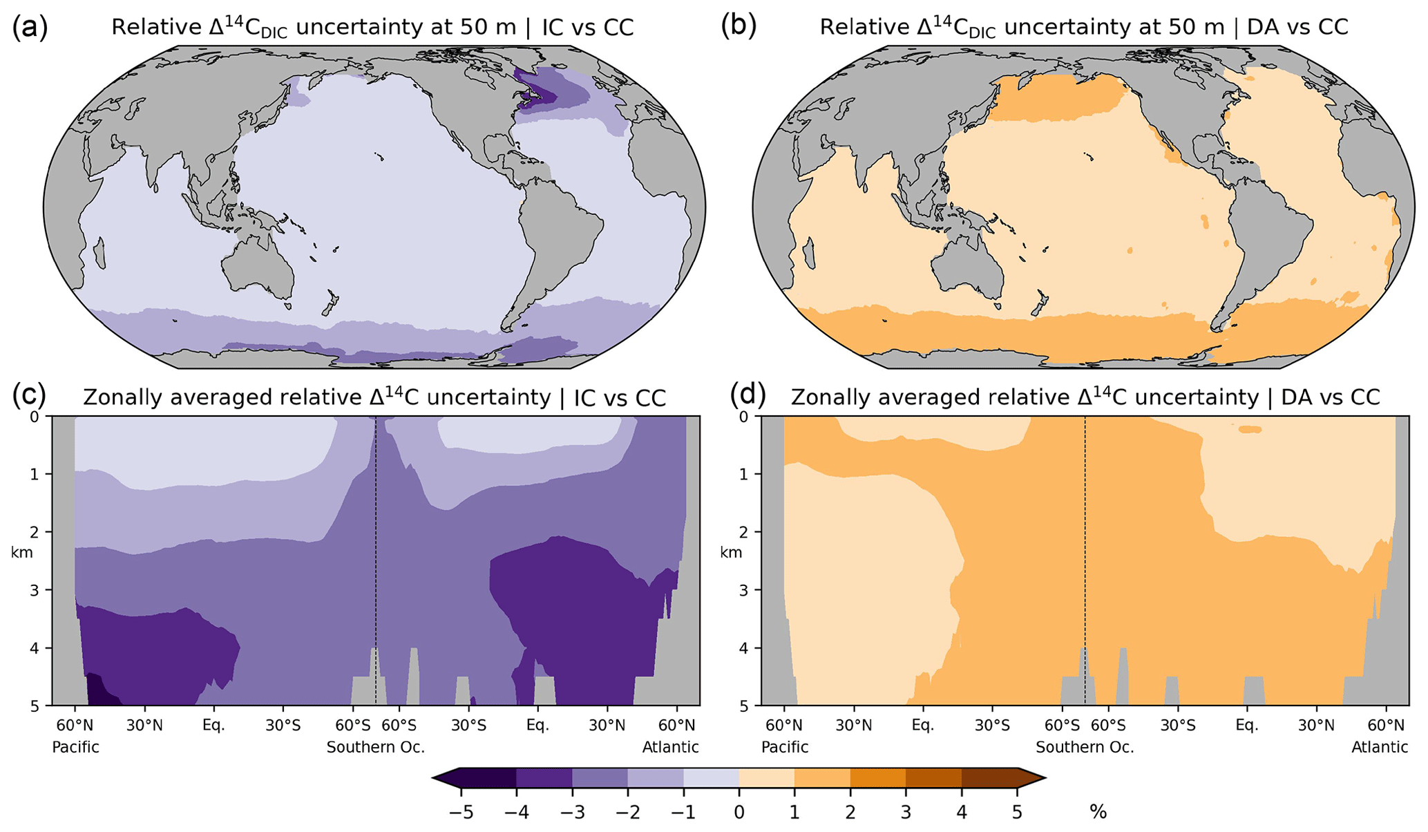
Figure 12Relative differences in preindustrial Δ14CDIC between the various simulation approaches: absolute values at a depth of 50 m depth (a, b) and in the Atlantic and Pacific (c, d) are shown. (a, c) No-fractionation (IC) approach versus complete 14C cycle (CC), (b, d) Δ14C approximation (DA) versus simulation CC.
We have added the carbon isotopes 13C and 14C to the marine biogeochemistry model REcoM3 and tested the implementation in long-term equilibrium simulations in which the configuration REcoM3p was coupled with the ocean general circulation model FESOM2.1. Regarding the carbon-isotopic composition of DIC (δ13CDIC and Δ14CDIC), our model results are largely consistent with marine δ13CDIC and Δ14CDIC fields reconstructed for the pre-anthropogenic period. The simulations also exhibit discrepancies, such as overly depleted δ13CDIC values in upwelling regions, overly steep vertical gradients of δ13CDIC and Δ14CDIC in the interior of the North Atlantic, and excessive depletion of Δ14CDIC in the interior of the North Pacific. To some extent, the inaccuracies of δ13CDIC indicate shortcomings in modelled organic carbon cycling. The radiocarbon results (Δ14CDIC) are insensitive to carbon cycle changes and reflect the rather shallow overturning circulation provided by our low-resolution ocean general circulation model test configuration with idealized repeat year climate forcing. As future simulations with a scientific focus will be carried out with considerably higher horizontal resolution and more realistic climate forcing, we expect some of the biases discussed in this study to decrease. These simulations should also consider transient boundary conditions of 13C and 14C, which provide additional benchmarks for the model. For these reasons we did not attempt to further tune REcoM3p here, e.g. by adjusting semi-empirical biogeochemical parameters such as gas transfer velocity or biogenic fractionation coefficients.
As Δ14CDIC is dominated by radioactive decay and transport processes, we have additionally explored the accuracy of two simplified modelling approaches that are more efficient than the complete consideration (CC) of the DI14C cycle. One approach (IC) neglects isotopic fractionation but still considers biological processes. The IC approach yields lower Δ14CDIC values than reconstructed for high-latitude surface waters and for deep and bottom waters. Another approach (DA) only considers the DI14C DIC ratio for constant and homogeneous DIC concentrations and further disregards the marine carbon cycle. It yields higher Δ14CDIC values than reconstructed for surface water, which mitigates the isotopic depletion in the deep sea, where the DA approach therefore better agrees with the reconstruction than the other approaches. The relative uncertainty between the comprehensive and simplified approaches is less than 5 %. Therefore, the simplified Δ14CDIC modelling approaches should be sufficiently accurate for radiocarbon dating of marine climate archives.
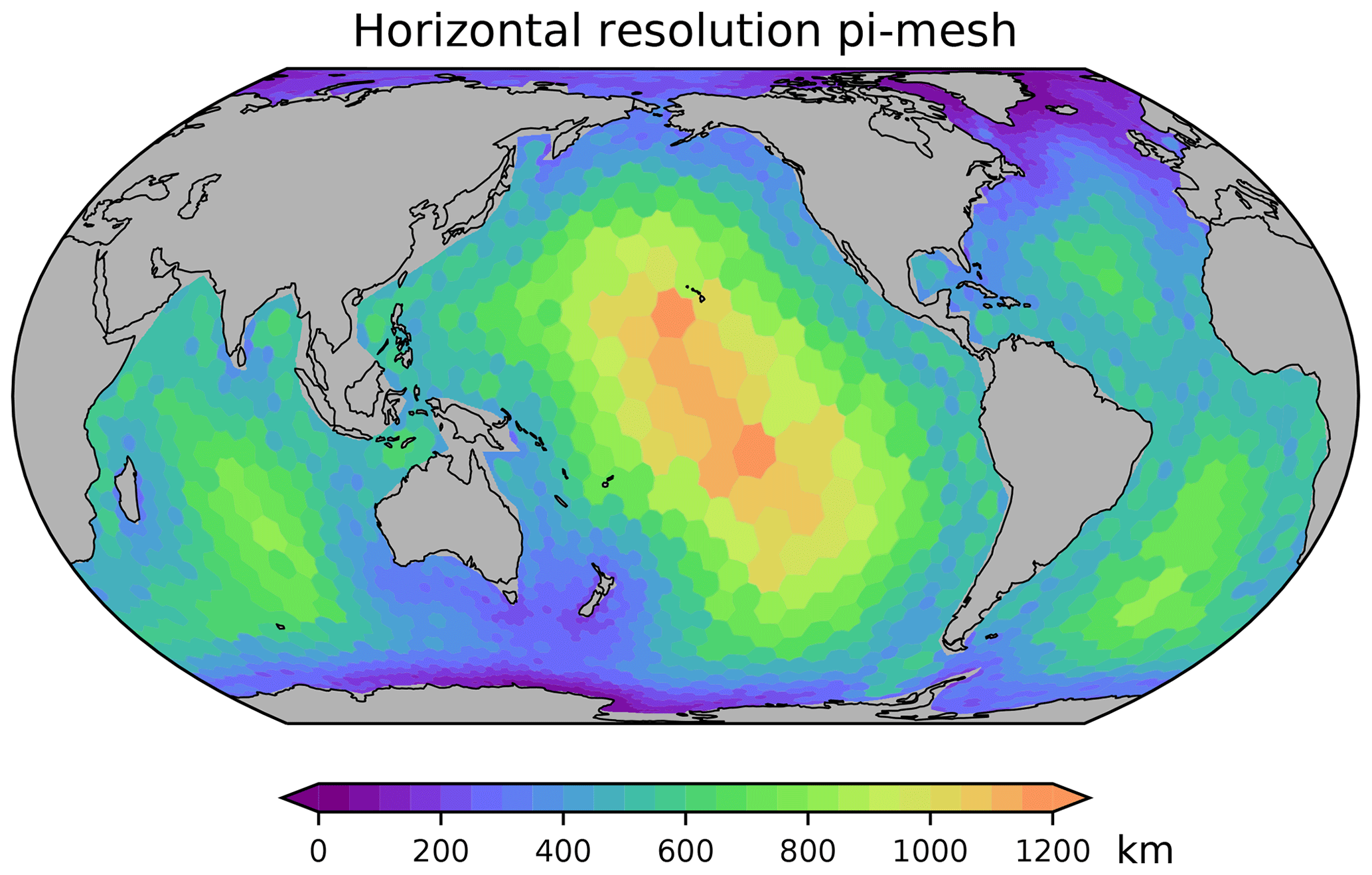
Figure A1Horizontal resolution of FESOM2.1-REcoM used in this study. The mesh has 3140 surface nodes. See also https://fesom.de/models/meshessetups/ (last access: 20 February 2024) for an impression of the bathymetry.
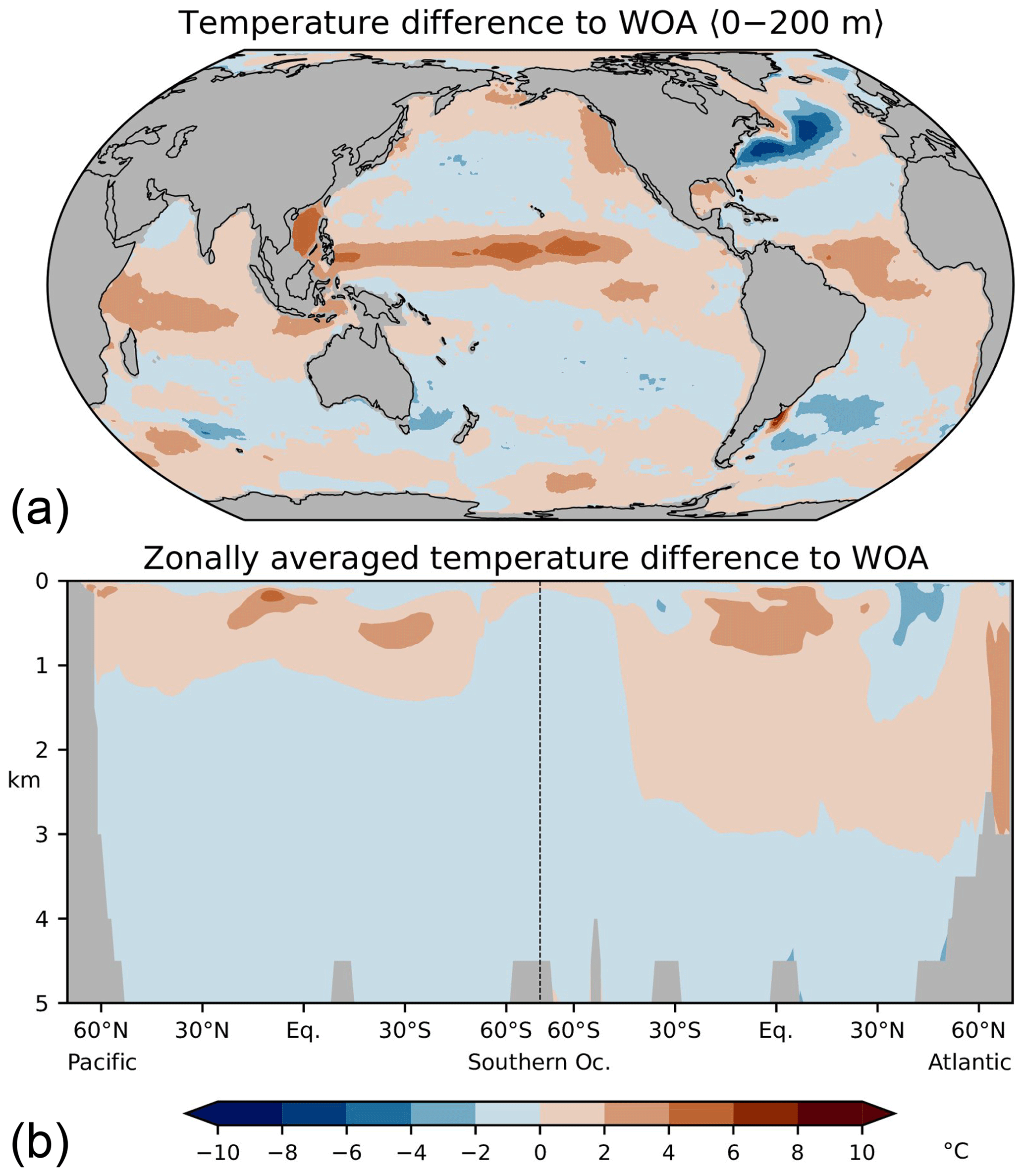
Figure A2Differences between simulated and observed (WOA09, Locarnini et al., 2010) temperatures, (a) averaged over the upper 200 m, (b) in the Atlantic and Pacific. See Scholz et al. (2019) for comparison with higher-resolution simulations.
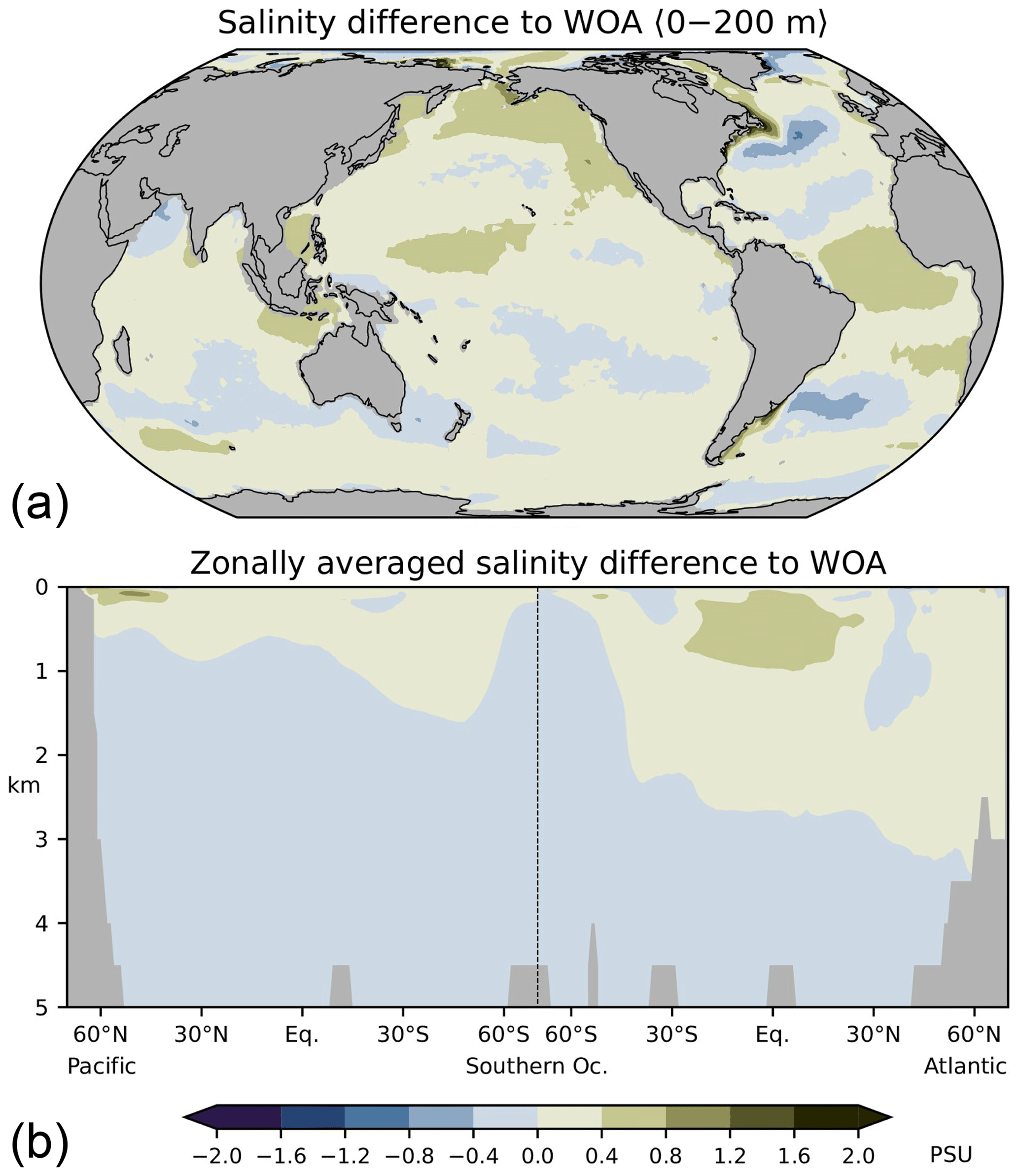
Figure A3Differences between simulated and observed (WOA09, Antonov et al., 2010) salinities, (a) averaged over the upper 200 m, (b) in the Atlantic and Pacific. See Scholz et al. (2019) for comparison with higher-resolution simulations.
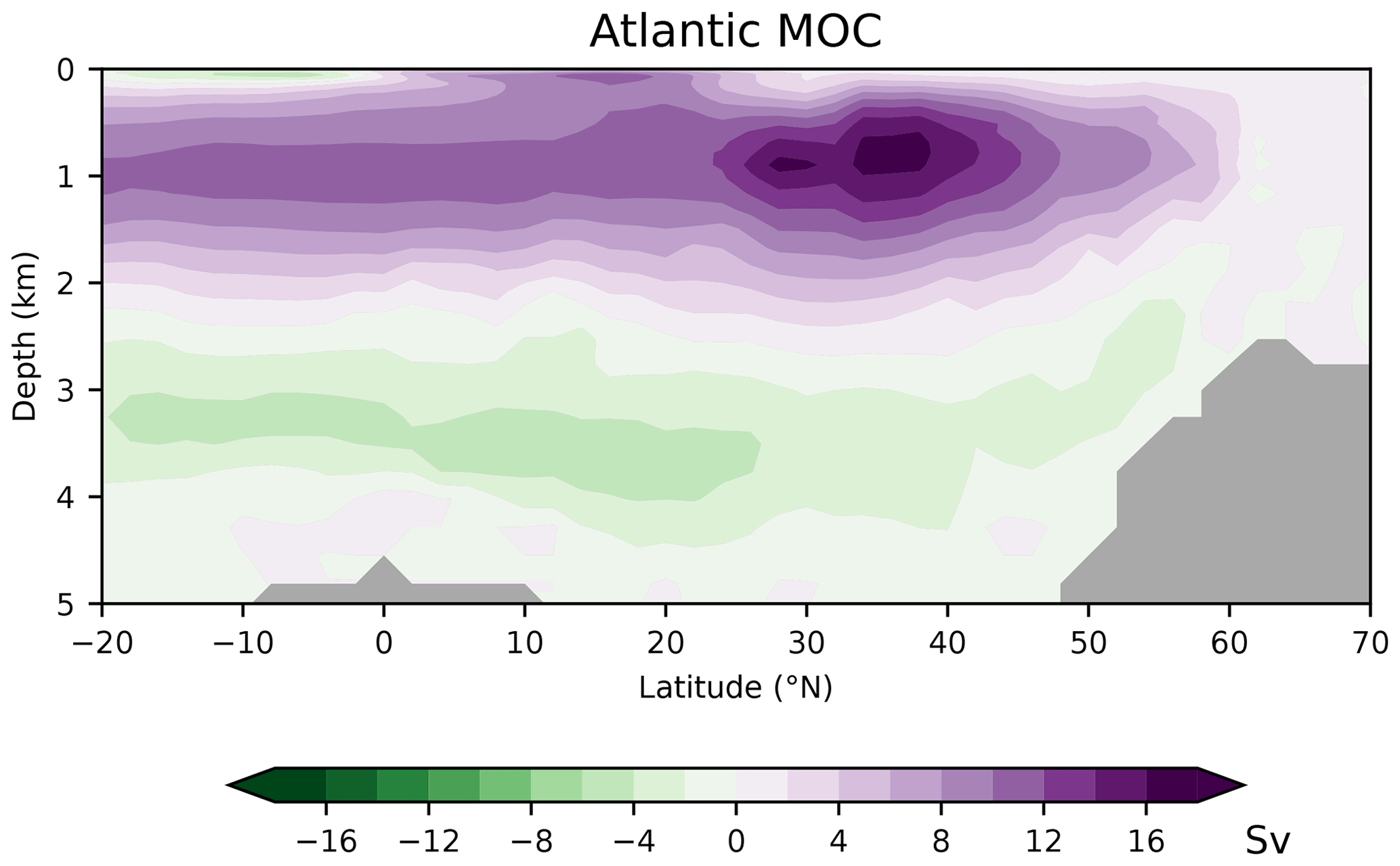
Figure A4Simulated meridional overturning circulation (MOC) in the Atlantic. See also Scholz et al. (2019, 2022) for comparison with higher-resolution simulations.
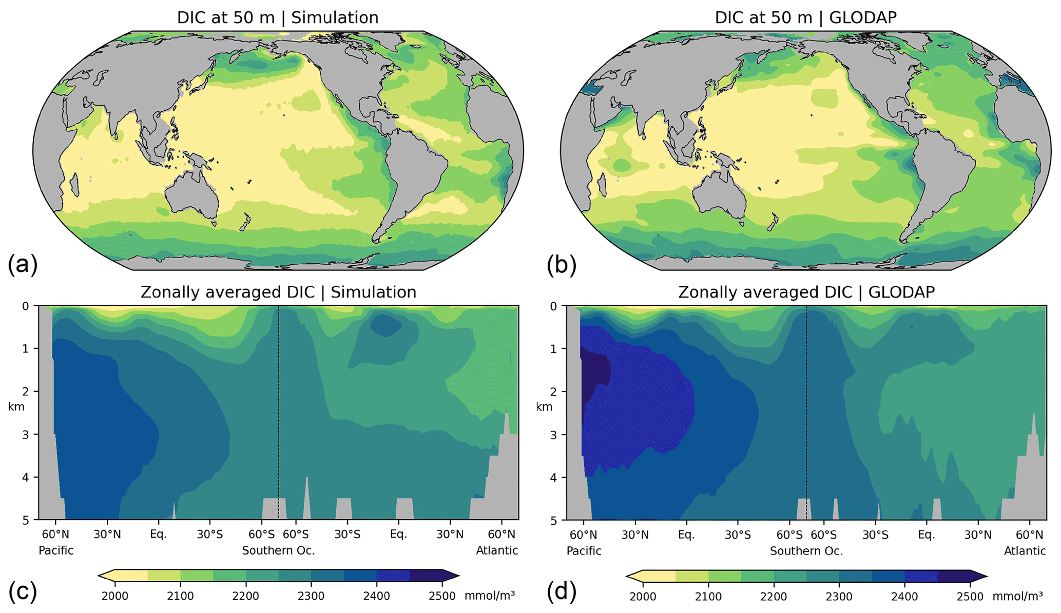
Figure A5Concentrations of dissolved inorganic carbon (DIC), (a, c) this study, (b, d) observations for 1972–2013 CE, normalized to the year 2002 (GLODAPv2, Key et al., 2015; Lauvset et al., 2016). (a, b) Concentrations at a depth of 50 m, (c, d) zonal-mean values in the Atlantic and Pacific. Model results are interpolated to the resolution of the observations (1° × 1° × 33 layers).
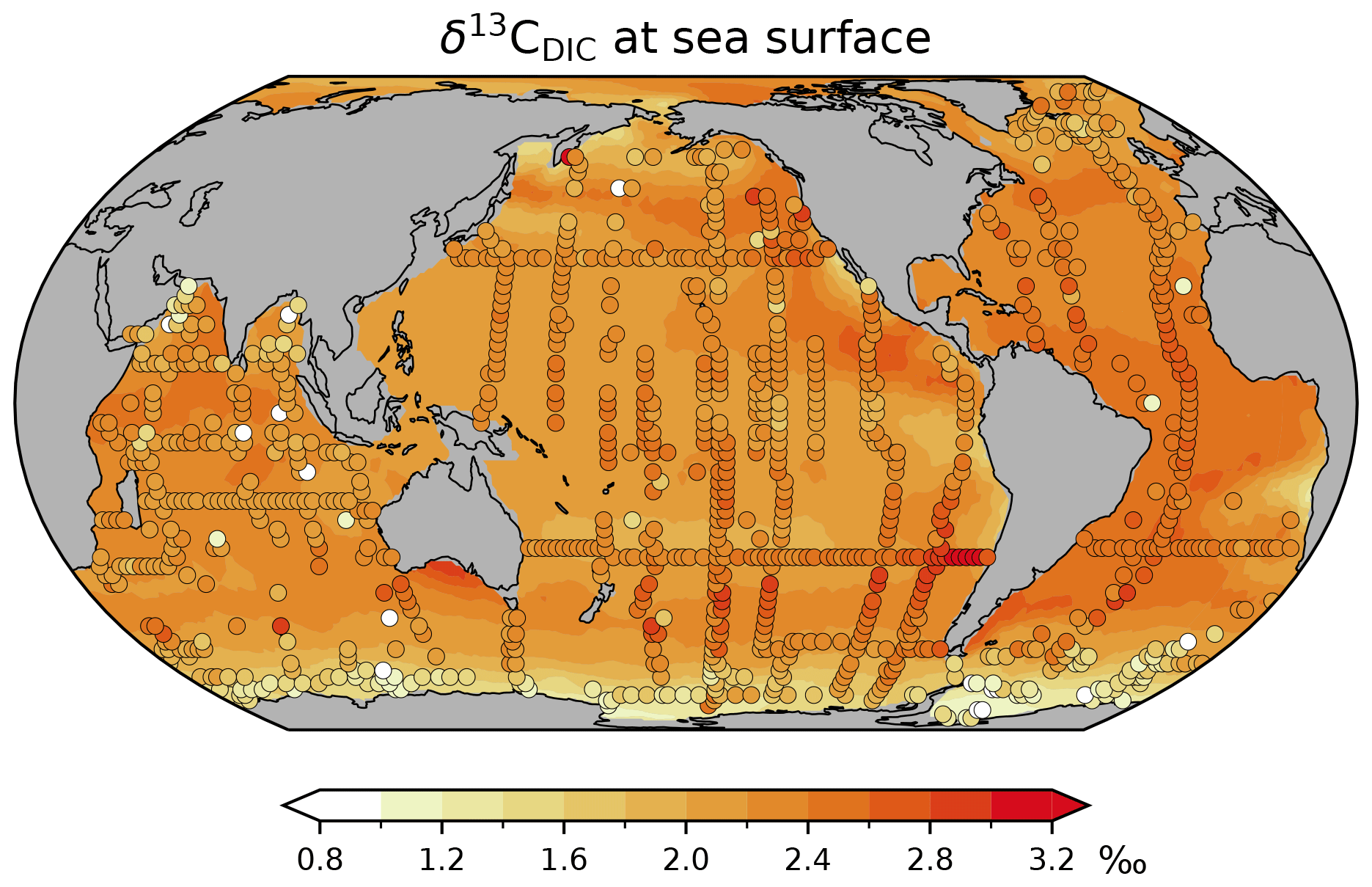
Figure A6Preindustrial δ13CDIC of surface water at a depth of about 18 m. Shaded areas: simulation CC; filled circles: reconstructed values by Kwon et al. (2022). Note that their reconstruction yields higher preindustrial δ13CDIC values than Eide et al. (2017b) in thermocline and intermediate waters of the Southern Hemisphere (see the discussion by Kwon et al., 2022).
The source code is available at https://doi.org/10.5281/zenodo.8169243 (Butzin, 2023).
MB developed the isotope code, conducted the simulations and prepared the manuscript with contributions from all co-authors.
The contact author has declared that none of the authors has any competing interests.
Publisher's note: Copernicus Publications remains neutral with regard to jurisdictional claims made in the text, published maps, institutional affiliations, or any other geographical representation in this paper. While Copernicus Publications makes every effort to include appropriate place names, the final responsibility lies with the authors.
We thank Dmitry Sidorenko for FESOM model support and Anne L. Morée and Andreas Schmittner for constructive reviews.
This work was supported by the German Federal Ministry of Education and Research (BMBF) via the PalMod project (grant no. 01LP1919A) which is part of the Research for Sustainability initiative FONA (https://www.fona.de, last access: 20 February 2024). Martin Butzin is additionally funded by the DFG-ANR project MARCARA (grant no. 490763579). Judith Hauck and Özgür Gürses were funded by the Initiative and Networking Fund of the Helmholtz Association (Helmholtz Young Investigator Group Marine Carbon and Ecosystem Feedbacks in the Earth System [MarESys], grant no. VH-NG-1301).
The article processing charges for this open-access publication were covered by the Alfred-Wegener-Institut Helmholtz-Zentrum für Polar- und Meeresforschung.
This paper was edited by Sergey Gromov and reviewed by Anne L. Morée and Andreas Schmittner.
Albani, S., Mahowald, N. M., Perry, A. T., Scanza, R. A., Zender, C. S. Heavens, N. G., Maggi, V., Kok, J. F., and Otto-Bliesner, B. L.: Improved dust representation in the Community Atmosphere Model, J. Adv. Model. Earth Sy., 6, 541–570, https://doi.org/10.1002/2013MS000279, 2014.
Antonov, J. I., Seidov, D., Boyer, T. P., Locarnini, R. A., Mishonov, A. V., Garcia, H. E., Baranova, O. K., Zweng, M. M., and Johnson, D. R.: World Ocean Atlas 2009, Volume 2: Salinity, Editor: Levitus, S., NOAA Atlas NESDIS 69, https://www.nodc.noaa.gov/OC5/WOA09/pubwoa09.html (last access: 20 February 2024), 2010.
Assonov, S., Groening, M., Fajgelj, A., Hélie, J.-F., and Hillaire-Marcel, C.: Preparation and characterisation of IAEA-603, a new primary reference material aimed at the VPDB scale realisation for δ13C and δ18O determination, Rapid Commun. Mass Sp., 34, e8867, https://doi.org/10.1002/rcm.8867, 2020.
Audi, G., Bersillon, O., Blachot, J., and Wapstra, A. H.: The Nubase evaluation of nuclear and decay properties, Nucl. Phys. A, 729, 3–128, https://doi.org/10.1016/j.nuclphysa.2003.11.001, 2003.
Aumont, O., Maier-Reimer, E., Blain, S., and Monfray, P.: An ecosystem model of the global ocean including Fe, Si, P colimitations, Global Biogeochem. Cycles, 17, 1060, https://doi.org/10.1029/2001GB001745, 2003.
Bé, M.-M. and Chechev, V. P.: 14C – Comments on evaluation of decay data, Laboratoire National Henri Becquerel, Gif-sur-Yvette, http://www.lnhb.fr/nuclides/C-14_com.pdf (last access: 20 February 2024), 2012.
Bidigare, R. R., Fluegge, A., Freeman, K. H., Hanson, K. L., Hayes, J. M., Hollander, D., Jasper, J. P., King, L. L., Laws, E. A., Milder, J., Millero, F. J., Pancost, R., Popp, B. N., Steinberg, P. A., and Wakeham, S. G.: Consistent fractionation of 13C in nature and in the laboratory: Growth-rate effects in some haptophyte algae, Global Biogeochem. Cycles, 11, 279–292, https://doi.org/10.1029/96GB03939, 1997.
Brandenburg, K. M., Rost, B., Van de Waal, D. B., Hoins, M., and Sluijs, A.: Physiological control on carbon isotope fractionation in marine phytoplankton, Biogeosciences, 19, 3305–3315, https://doi.org/10.5194/bg-19-3305-2022, 2022.
Broecker, W. S. and Maier-Reimer, E.: The influence of air and sea exchange on the carbon isotope distribution in the sea, Global Biogeochem. Cycles, 6, 315–320, https://doi.org/10.1029/92GB01672, 1992.
Broecker, W. S. and McGee, D.: The 13C record for atmospheric CO2: What is it trying to tell us?, Earth Planet. Sc. Lett., 368, 175–182, https://doi.org/10.1016/j.epsl.2013.02.029, 2013.
Broecker, W. S. and Peng, T.-H.: Tracers in the Sea, Eldigio Press, New York, 690 pp., 1982.
Buchanan, P. J., Matear, R. J., Chase, Z., Phipps, S. J., and Bindoff, N. L.: Ocean carbon and nitrogen isotopes in CSIRO Mk3L-COAL version 1.0: a tool for palaeoceanographic research, Geosci. Model Dev., 12, 1491–1523, https://doi.org/10.5194/gmd-12-1491-2019, 2019.
Buckley, M. W. and Marshall, J.: Observations, inferences, and mechanisms of the Atlantic Meridional Overturning Circulation: A review, Rev. Geophys., 54, 2015RG000493, https://doi.org/10.1002/2015RG000493, 2016.
Butzin, M.: FESOM2.1-REcoM3 source code with carbon isotopes (1.0.0), Zenodo [code], https://doi.org/10.5281/zenodo.8169243, 2023.
Ciais, P., Tagliabue, A., Cuntz, M., Bopp, L., Scholze, M., Hoffmann, G., Lourantou, A., Harrison, S. P., Prentice, I. C., Kelley, D. I., Koven, C. D., and Piao, S.: Large inert carbon pool in the terrestrial biosphere during the Last Glacial Maximum, Nat. Geosci., 5, 74–79, https://doi.org/10.1038/ngeo1324, 2012.
Claret, M., Sonnerup, R. E., and Quay, P. D.: A Next Generation Ocean Carbon Isotope Model for Climate Studies I: Steady State Controls on Ocean 13C, Global Biogeochem. Cycles, 35, e2020GB006757, https://doi.org/10.1029/2020GB006757, 2021.
Craig, H.: Carbon 13 in plants and the relationships between carbon 13 and carbon 14 variations in nature, J. Geol., 62, 115–149, 1954.
Danilov, S., Sidorenko, D., Wang, Q., and Jung, T.: The Finite-volumE Sea ice–Ocean Model (FESOM2), Geosci. Model Dev., 10, 765–789, https://doi.org/10.5194/gmd-10-765-2017, 2017.
Dentith, J. E., Ivanovic, R. F., Gregoire, L. J., Tindall, J. C., and Robinson, L. F.: Simulating stable carbon isotopes in the ocean component of the FAMOUS general circulation model with MOSES1 (XOAVI), Geosci. Model Dev., 13, 3529–3552, https://doi.org/10.5194/gmd-13-3529-2020, 2020.
Eide, M., Olsen, A., Ninnemann, U. S., and Eldevik, T.: A global estimate of the full oceanic 13C Suess effect since the preindustrial, Global Biogeochem. Cycles, 31, 2016GB005472, https://doi.org/10.1002/2016GB005472, 2017a.
Eide, M., Olsen, A., Ninnemann, U. S., and Johannessen, T.: A global ocean climatology of preindustrial and modern ocean δ13C, Global Biogeochem. Cycles, 31, 2016GB005473, https://doi.org/10.1002/2016GB005473, 2017b.
Fahrni, S. M., Southon, J. R., Santos, G. M., Palstra, S. W. L., Meijer, H. A. J., and Xu, X.: Reassessment of the and isotopic fractionation ratio and its impact on high-precision radiocarbon dating, Geochim. Cosmochim. Ac., 213, 330–345, https://doi.org/10.1016/j.gca.2017.05.038, 2017.
Fiadeiro, M. E.: Three-dimensional modeling of tracers in the deep Pacific Ocean, II. Radiocarbon and the circulation, J. Marine Res., 40, 537–550, 1982.
Freeman, K. H. and Hayes, J. M.: Fractionation of carbon isotopes by phytoplankton and estimates of ancient CO2 levels, Global Biogeochem. Cycles, 6, 185–198, https://doi.org/10.1029/92GB00190, 1992.
Frischknecht, T., Ekici, A., and Joos, F.: Radiocarbon in the land and ocean components of the Community Earth System Model, Global Biogeochem. Cycles, 36, e2021GB007042, https://doi.org/10.1029/2021GB007042, 2022.
Garcia, H. E., Locarnini, R. A., Boyer, T. P., Antonov, J. I., Baranova, O. K., Zweng, M. M., Reagan, J. R., and Johnson, D. R.: World Ocean Atlas 2013, Volume 4: Dissolved Inorganic Nutrients (Phosphate, Nitrate, Silicate), edited by: Levitus, S. and Mishonov, A., NOAA Atlas NESDIS 76, https://doi.org/10.7289/V5J67DWD (last access: 20 February 2024), 2014.
Garcia, H. E., Weathers, K., Paver, C. R., Smolyar, I., Boyer, T. P., Locarnini, R. A., Zweng, M. M., Mishonov, A. V., Baranova, O. K., Seidov, D., and Reagan, J. R.: World Ocean Atlas 2018, Volume 3: Dissolved Oxygen, Apparent Oxygen Utilization, and Oxygen Saturation, edited by: Mishonov, A., NOAA Atlas NESDIS 83, https://www.ncei.noaa.gov/access/world-ocean-atlas-2018/ (last access: 20 February 2024), 2019.
Graven, H., Lamb, E., Blake, D., and Khatiwala, S.: Future Changes in δ13C of Dissolved Inorganic Carbon in the Ocean, Earth's Future, 9, e2021EF002173, https://doi.org/10.1029/2021EF002173, 2021.
Griffies, S. M., Winton, M., Samuels, B., Danabasoglu, G., Yeager, S., Marsland, S., Drange., H., and Bentsen, M.: Datasets and protocol for the CLIVAR WGOMD Coordinated Ocean-sea ice Reference Experiments (COREs), WCRP Report No. 21/2012, https://eprints.soton.ac.uk/350257 (last access: 20 February 2024), 2012.
Gürses, Ö., Oziel, L., Karakuş, O., Sidorenko, D., Völker, C., Ye, Y., Zeising, M., Butzin, M., and Hauck, J.: Ocean biogeochemistry in the coupled ocean–sea ice–biogeochemistry model FESOM2.1–REcoM3, Geosci. Model Dev., 16, 4883–4936, https://doi.org/10.5194/gmd-16-4883-2023, 2023.
Heaton, T. J., Bard, E., Bronk Ramsey, C., Butzin, M., Köhler, P., Muscheler, R., Reimer, P. J., and Wacker, L.: Radiocarbon: A key tracer for studying Earth's dynamo, climate system, carbon cycle, and Sun, Science, 374, eabd7096, https://doi.org/10.1126/science.abd7096, 2021.
Hesse, T., Butzin, M., Bickert, T., and Lohmann, G.: A model-data comparison of δ13C in the glacial Atlantic Ocean, Paleoceanography, 26, PA3220, https://doi.org/10.1029/2010PA002085, 2011.
Holden, P. B., Edwards, N. R., Müller, S. A., Oliver, K. I. C., Death, R. M., and Ridgwell, A.: Controls on the spatial distribution of oceanic δ13CDIC, Biogeosciences, 10, 1815–1833, https://doi.org/10.5194/bg-10-1815-2013, 2013.
Jahn, A., Lindsay, K., Giraud, X., Gruber, N., Otto-Bliesner, B. L., Liu, Z., and Brady, E. C.: Carbon isotopes in the ocean model of the Community Earth System Model (CESM1), Geosci. Model Dev., 8, 2419–2434, https://doi.org/10.5194/gmd-8-2419-2015, 2015.
Jeltsch-Thömmes, A., Battaglia, G., Cartapanis, O., Jaccard, S. L., and Joos, F.: Low terrestrial carbon storage at the Last Glacial Maximum: constraints from multi-proxy data, Clim. Past, 15, 849–879, https://doi.org/10.5194/cp-15-849-2019, 2019.
Keeling, C. D.: The Suess effect: 13Carbon-14Carbon interrelations, Environ. Int., 2, 229–300, https://doi.org/10.1016/0160-4120(79)90005-9, 1979.
Keller, K. and Morel, F. M. M.: A model of carbon isotopic fractionation and active carbon uptake in phytoplankton, Marine Ecol. Prog. Ser., 182, 295–298, https://doi.org/10.3354/meps182295, 1999.
Key, R. M., Kozyr, A., Sabine, C. L., Lee, K., Wanninkhof, R., Bullister, J. L., Feely, R. A., Millero, F. J., Mordy, C., and Peng, T.-H.: A global ocean carbon climatology: Results from Global Data Analysis Project (GLODAP), Global Biogeochem. Cycles, 18, GB4031, https://doi.org/10.1029/2004GB002247, 2004.
Key, R. M., Olsen, A., Van Heuven, S., Lauvset, S. K., Velo, A., Lin, X., Schirnick, C., Kozyr, A., Tanhua, T., Hoppema, M., Jutterstrom, S., Steinfeldt, R., Jeansson, E., Ishi, M., Perez, F. F., and Suzuki, T.: Global Ocean Data Analysis Project, Version 2 (GLODAPv2), ORNL/CDIAC-162, ND-P093, https://doi.org/10.3334/CDIAC/OTG.NDP093_GLODAPv2, 2015.
Köhler, P., Fischer, H., Schmitt, J., and Munhoven, G.: On the application and interpretation of Keeling plots in paleo climate research – deciphering δ13C of atmospheric CO2 measured in ice cores, Biogeosciences, 3, 539–556, https://doi.org/10.5194/bg-3-539-2006, 2006.
Köhler, P.: Using the Suess effect on the stable carbon isotope to distinguish the future from the past in radiocarbon, Environ. Res. Lett., 11, 124016, https://doi.org/10.1088/1748-9326/11/12/124016, 2016.
Kutschera, W.: Applications of accelerator mass spectrometry, Int. J. Mass Sp., 349–350, 203–218, https://doi.org/10.1016/j.ijms.2013.05.023, 2013.
Kwon, E. Y., Timmermann, A., Tipple, B. J., and Schmittner, A.: Projected reversal of oceanic stable carbon isotope ratio depth gradient with continued anthropogenic carbon emissions, Commun. Earth Environ., 3, 1–12, https://doi.org/10.1038/s43247-022-00388-8, 2022.
Large, W. G. and Yeager, S. G.: The global climatology of an interannually varying air–sea flux data set, Clim. Dyn., 33, 341–364, https://doi.org/10.1007/s00382-008-0441-3, 2009 (data available at: https://data1.gfdl.noaa.gov/nomads/forms/core/COREv2/CNYF_v2.html, last access: 29 June 2021).
Lauvset, S. K., Key, R. M., Olsen, A., van Heuven, S., Velo, A., Lin, X., Schirnick, C., Kozyr, A., Tanhua, T., Hoppema, M., Jutterström, S., Steinfeldt, R., Jeansson, E., Ishii, M., Perez, F. F., Suzuki, T., and Watelet, S.: A new global interior ocean mapped climatology: the 1° × 1° GLODAP version 2, Earth Syst. Sci. Data, 8, 325–340, https://doi.org/10.5194/essd-8-325-2016, 2016.
Laws, E. A., Popp, B. N., Bidigare, R. R., Kennicutt, M. C., and Macko, S. A.: Dependence of phytoplankton carbon isotopic composition on growth rate and [CO2]aq: Theoretical considerations and experimental results, Geochim. Cosmochim. Ac., 59, 1131–1138, https://doi.org/10.1016/0016-7037(95)00030-4, 1995.
Laws, E. A., Bidigare, R. R., and Popp, B. N.: Effect of growth rate and CO2 concentration on carbon isotopic fractionation by the marine diatom Phaeodactylum tricornutum, Limnol. Oceanogr., 42, 1552–1560, https://doi.org/10.4319/lo.1997.42.7.1552, 1997.
Liu, B., Six, K. D., and Ilyina, T.: Incorporating the stable carbon isotope 13C in the ocean biogeochemical component of the Max Planck Institute Earth System Model, Biogeosciences, 18, 4389–4429, https://doi.org/10.5194/bg-18-4389-2021, 2021.
Locarnini, R. A., Mishonov, A. V., Antonov, J. I., Boyer, T. P., Garcia, H. E., Baranova, O. K., Zweng, M. M., and Johnson, D. R.: World Ocean Atlas 2009, Volume 1: Temperature, edited by: Levitus, S., NOAA Atlas NESDIS 68, https://www.nodc.noaa.gov/OC5/WOA09/pubwoa09.html (last access: 20 February 2024), 2010.
Lohmann, G., Butzin, M., Eissner, N., Shi, X., and Stepanek, C.: Abrupt Climate and Weather Changes Across Time Scales, Paleoceanogr. Paleocl., 35, e2019PA003782, https://doi.org/10.1029/2019PA003782, 2020.
Lorrain, A., Pethybridge, H., Cassar, N., Receveur, A., Allain, V., Bodin, N., Bopp, L., Choy, C. A., Duffy, L., Fry, B., Goni, N., Graham, B. S., Hobday, A. J., Logan, J. M., Ménard, F., Menkes, C. E., Olson, R. J., Pagendam, D. E., Point, D., Revill, A. T., Somes, C. J., and Young, J. W.: Trends in tuna carbon isotopes suggest global changes in pelagic phytoplankton communities, Global Change Biol., 26, 458–470, https://doi.org/10.1111/gcb.14858, 2020.
Lynch-Stieglitz, J., Adkins, J. F., Curry, W. B., Dokken, T., Hall, I. R., Herguera, J. C., Hirschi, J. J.-M., Ivanova, E. V., Kissel, C., Marchal, O., Marchitto, T. M., McCave, I. N., McManus, J. F., Mulitza, S., Ninnemann, U., Peeters, F., Yu, E.-F., and Zahn, R.: Atlantic Meridional Overturning Circulation During the Last Glacial Maximum, Science, 316, 66–69, https://doi.org/10.1126/science.1137127, 2007.
Matsumoto, K., Sarmiento, J. L., Key, R. M., Aumont, O., Bullister, J. L., Caldeira, K., Campin, J.-M., Doney, S. C., Drange, H., Dutay, J.-C., Follows, M., Gao, Y., Gnanadesikan, A., Gruber, N., Ishida, A., Joos, F., Lindsay, K., Maier-Reimer, E., Marshall, J. C., Matear, R. J., Monfray, P., Mouchet, A., Najjar, R., Plattner, G.-K., Schlitzer, R., Slater, R., Swathi, P. S., Totterdell, I. J., Weirig, M.-F., Yamanaka, Y., Yool, A., and Orr, J. C.: Evaluation of ocean carbon cycle models with data-based metrics, Geophys. Res. Lett., 31, L07303, https://doi.org/10.1029/2003GL018970, 2004.
Menking, J. A., Shackleton, S. A., Bauska, T. K., Buffen, A. M., Brook, E. J., Barker, S., Severinghaus, J. P., Dyonisius, M. N., and Petrenko, V. V.: Multiple carbon cycle mechanisms associated with the glaciation of Marine Isotope Stage 4, Nat. Commun., 13, 5443, https://doi.org/10.1038/s41467-022-33166-3, 2022.
Menviel, L., Mouchet, A., Meissner, K. J., Joos, F., and England, M. H.: Impact of oceanic circulation changes on atmospheric δ13CO2, Global Biogeochem. Cycles, 29, 1944–1961, https://doi.org/10.1002/2015GB005207, 2015.
Morée, A. L., Schwinger, J., Ninnemann, U. S., Jeltsch-Thömmes, A., Bethke, I., and Heinze, C.: Evaluating the biological pump efficiency of the Last Glacial Maximum ocean using δ13C, Clim. Past, 17, 753–774, https://doi.org/10.5194/cp-17-753-2021, 2021.
Mouchet, A., The ocean bomb radiocarbon inventory revisited, Radiocarbon, 55, 1580–1594, https://doi.org/10.1017/S0033822200048505, 2013.
Munhoven, G.: Model of Early Diagenesis in the Upper Sediment with Adaptable complexity – MEDUSA (v. 2): a time-dependent biogeochemical sediment module for Earth system models, process analysis and teaching, Geosci. Model Dev., 14, 3603–3631, https://doi.org/10.5194/gmd-14-3603-2021, 2021.
Orr, J. C., Najjar, R. G., Aumont, O., Bopp, L., Bullister, J. L., Danabasoglu, G., Doney, S. C., Dunne, J. P., Dutay, J.-C., Graven, H., Griffies, S. M., John, J. G., Joos, F., Levin, I., Lindsay, K., Matear, R. J., McKinley, G. A., Mouchet, A., Oschlies, A., Romanou, A., Schlitzer, R., Tagliabue, A., Tanhua, T., and Yool, A.: Biogeochemical protocols and diagnostics for the CMIP6 Ocean Model Intercomparison Project (OMIP), Geosci. Model Dev., 10, 2169–2199, https://doi.org/10.5194/gmd-10-2169-2017, 2017.
Popp, B. N., Laws, E. A., Bidigare, R. R., Dore, J. E., Hanson, K. L., and Wakeham, S. G.: Effect of Phytoplankton Cell Geometry on Carbon Isotopic Fractionation, Geochim. Cosmochim. Ac., 62, 69–77, https://doi.org/10.1016/S0016-7037(97)00333-5, 1998.
Quay, P. D., Tilbrook, B., and Wong, C. S.: Oceanic Uptake of Fossil Fuel CO2: Carbon-13 Evidence, 256, 74–79, https://doi.org/10.1126/science.256.5053.74, 1992.
Rafter, P. A., Gray, W. R., Hines, S. K. V., Burke, A., Costa, K. M., Gottschalk, J., Hain, M. P., Rae, J. W. B., Southon, J. R., Walczak, M. H., Yu, J., Adkins, J. F., and DeVries, T.: Global reorganization of deep-sea circulation and carbon storage after the last ice age, Sci. Adv., 8, eabq5434, https://doi.org/10.1126/sciadv.abq5434, 2022.
Rau, G. H., Riebesell, U., and Wolf-Gladrow, D.: A model of photosynthetic 13C fractionation by marine phytoplankton based on diffusive molecular CO2 uptake, Marine Ecol. Prog. Ser., 133, 275–285, https://doi.org/10.3354/meps133275, 1996.
Rau, G. H., Riebesell, U., and Wolf-Gladrow, D.: CO2aq-dependent photosynthetic 13C fractionation in the ocean: A model versus measurements, Global Biogeochem. Cycles, 11, 267–278, https://doi.org/10.1029/97GB00328, 1997.
Šavrič, B., Patterson, T., and Jenny, B.: The Equal Earth map projection, Int. J. Geogr. Inf. Sci., 33, 454–465, https://doi.org/10.1080/13658816.2018.1504949, 2019.
Schmittner, A., Gruber, N., Mix, A. C., Key, R. M., Tagliabue, A., and Westberry, T. K.: Biology and air–sea gas exchange controls on the distribution of carbon isotope ratios (δ13C) in the ocean, Biogeosciences, 10, 5793–5816, https://doi.org/10.5194/bg-10-5793-2013, 2013.
Schmittner, A., Bostock, H. C., Cartapanis, O., Curry, W. B., Filipsson, H. L., Galbraith, E. D., Gottschalk, J., Herguera, J. C., Hoogakker, B., Jaccard, S. L., Lisiecki, L. E., Lund, D. C., Martínez-Méndez, G., Lynch-Stieglitz, J., Mackensen, A., Michel, E., Mix, A. C., Oppo, D. W., Peterson, C. D., Repschläger, J., Sikes, E. L., Spero, H. J., and Waelbroeck, C.: Calibration of the carbon isotope composition (δ13C) of benthic foraminifera, Paleoceanography, 32, 512–530, https://doi.org/10.1002/2016PA003072, 2017.
Scholz, P., Sidorenko, D., Gurses, O., Danilov, S., Koldunov, N., Wang, Q., Sein, D., Smolentseva, M., Rakowsky, N., and Jung, T.: Assessment of the Finite-volumE Sea ice-Ocean Model (FESOM2.0) – Part 1: Description of selected key model elements and comparison to its predecessor version, Geosci. Model Dev., 12, 4875–4899, https://doi.org/10.5194/gmd-12-4875-2019, 2019.
Scholz, P., Sidorenko, D., Danilov, S., Wang, Q., Koldunov, N., Sein, D., and Jung, T.: Assessment of the Finite-VolumE Sea ice–Ocean Model (FESOM2.0) – Part 2: Partial bottom cells, embedded sea ice and vertical mixing library CVMix, Geosci. Model Dev., 15, 335–363, https://doi.org/10.5194/gmd-15-335-2022, 2022.
Skinner, L. C. and Bard, E.: Radiocarbon as a Dating Tool and Tracer in Paleoceanography, Rev. Geophys., 60, e2020RG000720, https://doi.org/10.1029/2020RG000720, 2022.
Skinner, L., Primeau, F., Jeltsch-Thömmes, A., Joos, F., Köhler, P., and Bard, E.: Rejuvenating the ocean: mean ocean radiocarbon, CO2 release, and radiocarbon budget closure across the last deglaciation, Clim. Past, 19, 2177–2202, https://doi.org/10.5194/cp-19-2177-2023, 2023.
Steele, M., Morley, R., and Ermold, W.: PHC: A Global Ocean Hydrography with a High-Quality Arctic Ocean, J. Climate, 14, 2079–2087, https://doi.org/10.1175/1520-0442(2001)014<2079:PAGOHW>2.0.CO;2, 2001.
Stuiver, M. and Polach, H. A.: Discussion; reporting of C-14 data, Radiocarbon, 19, 355–363, 1977.
Suess, H. E.: Radiocarbon Concentration in Modern Wood, Science, 122, 415–417, https://doi.org/10.1126/science.122.3166.415-a, 1955.
Tagliabue, A. and Bopp, L.: Towards understanding global variability in ocean carbon-13, Global Biogeochem. Cycles, 22, GB1025, https://doi.org/10.1029/2007GB003037, 2008.
Tagliabue, A., Mtshali, T., Aumont, O., Bowie, A. R., Klunder, M. B., Roychoudhury, A. N., and Swart, S.: A global compilation of dissolved iron measurements: focus on distributions and processes in the Southern Ocean, Biogeosciences, 9, 2333–2349, https://doi.org/10.5194/bg-9-2333-2012, 2012.
Tjiputra, J. F., Schwinger, J., Bentsen, M., Morée, A. L., Gao, S., Bethke, I., Heinze, C., Goris, N., Gupta, A., He, Y.-C., Olivié, D., Seland, Ø., and Schulz, M.: Ocean biogeochemistry in the Norwegian Earth System Model version 2 (NorESM2), Geosci. Model Dev., 13, 2393–2431, https://doi.org/10.5194/gmd-13-2393-2020, 2020.
Toggweiler, J. R., Dixon, K., and Bryan, K.: Simulations of radiocarbon in a coarse-resolution world ocean model: 1. Steady state prebomb distributions, J. Geophys. Res., 94, 8217–8242, https://doi.org/10.1029/JC094iC06p08217, 1989.
Tschumi, T., Joos, F., Gehlen, M., and Heinze, C.: Deep ocean ventilation, carbon isotopes, marine sedimentation and the deglacial CO2 rise, Clim. Past, 7, 771–800, https://doi.org/10.5194/cp-7-771-2011, 2011.
Verwega, M.-T., Somes, C. J., Schartau, M., Tuerena, R. E., Lorrain, A., Oschlies, A., and Slawig, T.: Description of a global marine particulate organic carbon-13 isotope data set, Earth Syst. Sci. Data, 13, 4861–4880, https://doi.org/10.5194/essd-13-4861-2021, 2021.
Wanninkhof, R.: Relationship between wind speed and gas exchange over the ocean revisited: Gas exchange and wind speed over the ocean, Limnol. Oceanogr.-Methods, 12, 351–362, https://doi.org/10.4319/lom.2014.12.351, 2014.
Ye, Y., Munhoven, G., Köhler, P., Butzin, M., Hauck, J., Gürses, Ö., and Völker, C.: FESOM2.1-REcoM3-MEDUSA2: an ocean-sea ice-biogeochemistry model coupled to a sediment model, Geosci. Model Dev. Discuss. [preprint], https://doi.org/10.5194/gmd-2023-181, in review, 2023.
Young, J. N., Bruggeman, J., Rickaby, R. E. M., Erez, J., and Conte, M.: Evidence for changes in carbon isotopic fractionation by phytoplankton between 1960 and 2010, Global Biogeochem. Cycles, 27, 505–515, https://doi.org/10.1002/gbc.20045, 2013.
Zhang, J., Quay, P. D., and Wilbur, D. O.: Carbon isotope fractionation during gas-water exchange and dissolution of CO2, Geochim. Cosmochim. Ac., 59, 107–114, https://doi.org/10.1016/0016-7037(95)91550-D, 1995.
Ziveri, P., Stoll, H., Probert, I., Klaas, C., Geisen, M., Ganssen, G., and Young, J.: Stable isotope `vital effects' in coccolith calcite, Earth Planet. Sc. Lett., 210, 137–149, https://doi.org/10.1016/S0012-821X(03)00101-8, 2003.