2.1 Model evaluation and sensitivity experiments based on observed CRFs (obsclim)

The experiments described in this section are all based on observational (factual) climate data, coastal water levels, and atmospheric CO₂ as well as CH₄ concentrations including observed trends. The only exception are the sensitivity experiments where CO₂ concentrations are fixed at 1901 levels (1901co2). However, as these experiments only deviate in this one aspect from the factual CRF they are also described by the obsclim CRF specifier but the 1901co2 sensitivity specifier to indicate the deviation. So all experiments described in this section share the common obsclim CRF specifier in the file names. In contrast, all experiments described in Sect. 2.2 can be identified by the counterclim specifier in the names of the output files containing the impact model simulations.

2.1.1 Default evaluation experiments based on observed CRFs (obsclim)

In this first part of Sect. 2.1 we describe the default ISIMIP3a experiments (sensitivity specifier in the file names set to default) that are based on the standard observed climate-related forcings (obsclim, see CRF part of Table 1) in combination with different assumptions regarding direct human forcings (histsoc, 2015soc, 1901soc, and nat) illustrated in Fig. 1.

Standard evaluation experiment (obsclim + histsoc; default). The first set of observation-based simulations is dedicated to impact model evaluation, i.e., to test our ability to reproduce and explain observed long-term changes or variations in impact indicators such as crop yields, river discharge, changes in natural vegetation carbon, vegetation types, and peatland moisture conditions. To this end, we provide the climate-related (obsclim), direct human (histsoc), and static geographical forcings listed in Table 1. They are described in more detail in Sects. 3 and 4.

For impact model simulations that require a spin-up to, e.g., balance carbon stocks, 100 years of climate data (spinclim) are provided that represent stable 1900 climate conditions. The spinclim data are equivalent to the first 100 years of the counterfactual climate data that are described in Sect. 3.1. If more than 100 years of spin-up are needed, the spinclim data can be repeated as often as needed. For the spin-up, CO₂ concentrations and direct human forcing should be kept constant at 1850 levels. To get to the historical reporting period starting in 1901, modelers should simulate a transition period from 1850 to 1900 using spinclim climate data and the observed increase in CO₂ concentrations and historical changes in socioeconomic forcings (from 1850–1900).

The temporal coverage of the evaluation experiment is limited to 1961–2010 in the marine ecosystems and fisheries sector due to the availability of reanalysis-based oceanic forcing data (Liu et al., 2021). As a spin-up + transition period for the “obsclim + histsoc; default” experiments starting in 1961 the models should be run through six cycles of 1961–1980 1955-riverine-input CRFs (120 years, see Table 1) assuming reconstructed fishing efforts from 1861–1960 and constant 1861 levels before during 1841–1860 (see Table 1 and Fig. 3 in Sect. 4.9). If more years of spin-up are required, additional cycles of the 1961–1980 1955-riverine-input CRFs should be added, assuming constant 1861 fishing efforts.

Table 1Climate-related, direct human, and static geographic forcing data provided for the model evaluation and sensitivity experiments within ISIMIP3a. The CRFs are grouped according to the definition of the default obsclim CRF (30 arcmin for the atmospheric data and 15 arcmin for the oceanic data); the higher-resolution 30arcsec, 90arcsec, 300arcsec, and 1800arcsec atmospheric CRF; the lower-resolution 60arcmin oceanic CRF; and the 1955-riverine-input oceanic CRF for the sensitivity experiments. The listed set of DHFs defines the histsoc setup.

Download XLSX

Fixed 2015 direct human forcing (obsclim + 2015soc; default). To allow for the quantification of the effect of historical changes in direct human forcings, ISIMIP3a also contains an experiment where all direct human forcings are held constant at 2015 levels. The difference between the evaluation run described above and this baseline simulation can be considered the impact of changes in direct human forcings. In this sense the experiment allows for the attribution of observed changes in the natural, human, and managed systems to changes in DHF after 2015. In addition, the simulated changes in models' output variables can be considered the “pure effects of climate-related forcings”, conditional on present-day socioeconomic conditions. The experiment is also introduced because not all impact models can account for varying direct human forcings but rather assume fixed “present-day” conditions. All modeling teams are asked to do this experiment even if they are able to account for varying direct human forcings to generate one set of impact simulations that can be integrated across all participating models from different sectors or where all simulations from one sector can be compared. If a spin-up is required, it should be based on the spinclim data as described above but fixed 2015 direct human forcings.

Fixed 1901 direct human forcing baseline (obsclim + 1901soc; default). Fixing direct human forcings at 1901 levels is an alternative approach to quantify (i) the effects of direct human forcings when comparing these baseline simulations to the evaluation run and (ii) the “pure effect of observed change in climate-related systems”, conditional on socioeconomic conditions observed before the onset of this change. As such the experiment is the counterfactual baseline when aiming for the attribution of observed changes in natural, human, and managed systems to observed changes in direct human forcings instead of the attribution to observed changes in climate-related systems based on the analogous “counterfactual + histsoc; default” experiment described in Sect. 2.2. Both experiments consider changes in direct human forcings or climate-related systems from 1901 levels, respectively. Because of the low levels of direct human forcings in 1901, this experiment is similar to the sector-specific “nat” experiment that includes no direct human forcings whatsoever (see below). However, while the fully naturalized nat run is suitable for dynamic vegetation models from the biomes sector that simulate land cover by vegetation on their own, models in other sectors need land cover as an input. As this information is not available for pristine conditions, we introduce the 1901soc scenario such that models in the water sector can use land cover data approximately representative of 1901 conditions to describe a situation with minor human influences. If a spin-up is required, it should be based on the spinclim data as described above but fixed 1901 direct human forcings.

No direct human forcing baseline (obsclim + nat; default). To estimate the full effect of 2015 levels of DHF we also introduce a baseline nat experiment that does not consider any DHFs but a natural state of the world. Then the difference to the “obsclim + 2015soc; default” experiment can be considered the effect of 2015 levels of DHF. The comparison to the “obsclim + histsoc; default” experiment allows for the attribution of observed changes in the natural, human, and managed systems to historical changes in the DHF. Trends in the “obsclim + nat; default” run only represent the impacts historical changes in the climate-related forcings would have had on an otherwise natural state of the world. While the 1901soc conditions may be similar to nat conditions, trends in the “obsclim + 1901soc; default” run may not only be induced by historical changes in the CRFs but could also represent lagged responses to changes in DHFs during the transition period. The nat experiment can also be used to quantify the natural carbon sequestration potential of natural vegetation without any management or land use as an important counterfactual baseline to assess the addition of carbon sequestration measures. The nat experiment is sector-specific for the biomes–peat and marine ecosystems–fisheries sectors. If a spin-up is required in the biomes and peat sector, it should be based on the spinclim data as described above but assuming no direct human forcings. In the marine ecosystems and fisheries sector the spin-up should be based on the 1955-riverine-input CRF as described for the “obsclim + histsoc; default” section but assuming no DHF, i.e., no fishing efforts.

2.1.2 Sensitivity experiments based on observed CRFs (obsclim)

This second part of Sect. 2.1 is dedicated to the different sensitivity experiments described as deviations from the default cases described in Sect. 2.1.1. Instead of the default specifier, all experiments described here are labeled by sensitivity specifiers indicating their deviation from the default cases. The experiments listed here are not explicitly depicted in Fig. 1.

High- and low-resolution sensitivity experiments (obsclim + histsoc; 30arcsec, 90arcsec, 300arcsec, 1800arcsec, and 60arcmin). To test whether high-resolution atmospheric climate data improve the climate impact model simulations, we also provide observational atmospheric forcing data at 30^′′ (30arcsec), 90^′′ (90arcsec), and 300^′′ (300arcsec) resolution as well as atmospheric forcings at the original 1800^′′ resolution but derived from the 30^′′ (∼1 km) data (1800arcsec). In addition, the oceanic data (original resolution of 0.25^∘) are upscaled to 1^∘ to also test the sensitivity of the impact simulations to this modification (60arcmin).

The 30^′′ atmospheric data (1979–2016) are derived from a topographic downscaling of the observational W5E5 data (resolution of 0.5^∘) that particularly corrects for systematic effects induced by orographic details not represented in global reanalyses (CHELSA-W5E5, see Sect. 3.1). The dataset comprises daily mean precipitation, daily mean surface downwelling shortwave radiation, daily mean near-surface air temperature, daily maximum near-surface air temperature, and daily minimum near-surface air temperature (see Table 5). We additionally provide simple approaches to downscale surface downwelling longwave radiation, near-surface relative humidity, air pressure, and near-surface wind speed (see Sect. 3.1). Given the considerable storage capacities required by daily 1 km × 1 km data and constraints on data handling and download, we also aggregate the CHELSA-W5E5 data to 90^′′ (∼3 km), 300^′′ (∼10 km), and 1800${}^{\prime \prime }=\mathrm{0.5}$^∘ (∼60 km) to determine which resolution is required to improve the impact model simulations compared to observed impact indicators. The evaluation of these historical sensitivity experiments will inform future downscaling activities for GCM climate forcing data including future projections. The 1800arcsec experiment is included as a reference, as the aggregated CHELSA-W5E5 data differ from the standard W5E5 data at the same resolution (see Sect. 3.1). So far the experiments have been added to the agriculture, lakes, global and regional water, regional forests, terrestrial biodiversity, and labor protocol. However, they may be added to other sectors, too. The inclusion of the experiment is only constrained by the restricted set of variables included in CHELSA-W5E5. We do not provide spin-up data for the experiments. This means that models requiring a spin-up currently cannot perform the experiments. We will work on a solution on demand.

In contrast to the experiment testing the sensitivity of the impact simulations to a higher resolution of the atmospheric CRFs, the associated sensitivity experiment for the marine ecosystems and fisheries sector is not based on higher- but on lower-resolution oceanic data. While the default obsclim oceanic forcing data are derived by interpolating the observation-based historical ocean simulations from a tripolar 0.25^∘ grid to a regular 0.25^∘ grid (see Sect. 3.4), the CRFs for the sensitivity experiment are derived by aggregating the default obsclim data to a regular 1.0^∘ grid (60arcmin). Evaluating the 1.0^∘ resolution is of interest because this is the resolution of the oceanic forcing data in ISIMIP3b. The low-resolution simulations could either start from the end of the simulations of the transition period of the associated higher-resolution runs (“obsclim + histsoc; default”) or starting conditions could be newly generated by following the spin-up + transition procedure of the “obsclim + histsoc; default” experiment but using the low-resolution 1955-riverine-input CRF from the years 1961–1980.

The low-resolution sensitivity experiment (obsclim + nat; 60arcmin) for the marine ecosystems and fisheries sector is analogous to the “obsclim + nat; default” experiment described further above but using the lower-resolution oceanic CRF (60arcmin). The difference between this experiment and the “obsclim + histsoc; 60arcmin” sensitivity experiment can be considered the effect of the historical changes in DHF as estimated using lower-resolution CRF, and comparison with the same difference in the default experiments then indicates how the estimate of this effect depends on the resolution of the oceanic forcing. The simulations could either start from the end of the simulations of the transition period of the associated higher-resolution runs (“obsclim + nat; default”) or starting conditions could be newly generated by following the spin-up + transition procedure of the “obsclim + nat; default” experiment but using the low-resolution 1955-riverine-input CRF from the years 1961–1980.

CO₂ sensitivity experiments (obsclim + histsoc, obsclim + 2015soc, or obsclim + 1901soc; 1901co2). To quantify the pure effect of the historical increase in atmospheric CO₂ concentrations on vegetation leaf gas exchange and follow-on effects such as on carbon stocks, water use efficiency, and vegetation distribution, we introduced three sensitivity experiments where atmospheric CO₂ concentrations are held constant at 1901 levels (296.13 ppm) in contrast to the default obsclim + histsoc, obsclim + 2015soc, or obsclim + 1901soc experiments, respectively, where atmospheric CO₂ concentrations are assumed to increase according to observations. The effect is known as CO₂ fertilization through an increase in the photosynthesis rate of plants and limited leaf transpiration (increase in water use efficiency), enabling a more efficient uptake of carbon by the plants. Comparing the “obsclim + histsoc; default” experiment to the “obsclim + histsoc, 1901soc” experiment can be considered attributing historical changes in natural, human, and managed systems to historical changes in CO₂ concentrations as a single component of the changes in climate-related systems. The experiment is included in the protocols of the sector for agriculture, terrestrial biodiversity, biomes, fire, lakes (global and local), permafrost, and peat and water (global and regional). A potentially required spin-up should be identical to the spin-up for the associated default experiments using the transition period 1850–1900 to reach the 1901 CO₂ level.

Water management sensitivity experiment (obsclim + histsoc, obsclim + 2015soc; nowatermgt). In this “no water management” experiment, models are run assuming no irrigation, no human water abstraction, no dams or reservoirs, and no seawater desalination, while other direct human forcings such as land use changes are considered according to histsoc or 2015soc. By comparison to the default experiments, the simulations allow for a quantification of the pure effects of dedicated water management measures on, e.g., discharge. When comparing “obsclim + histsoc, nowatermgt” to “obsclim + histsoc; default” this can be considered attributing observed changes in natural, human, or managed systems to (changes in) water management. The sensitivity experiment has been introduced into the global and regional water sector protocols. If a spin-up is required, it should be done similar to the spin-up for the associated default experiments but assuming no water management.

Irrigation sensitivity experiment (obsclim + histsoc, 1901irr). In this “no irrigation expansion” experiment, models are run assuming irrigation extent and irrigation water use efficiencies fixed at the year 1901, while other direct human forcings such as land use changes and water management categories are considered according to histsoc or 2015soc. By comparison to the default experiments, the simulations allow for a quantification of the pure effects of historical irrigation expansion (i.e., the attribution of historical changes in natural, human, or managed systems to changes in irrigation compared to 1901). The sensitivity experiment has been introduced into the global water and biome sector protocols. If a spin-up is required, it should be done similar to the spin-up for the associated default experiments but assuming no irrigation expansion. This experiment is designed such that its outcomes are comparable to those of the Irrigation Impacts Model Intercomparison Project (IRRMIP; https://hydr.vub.be/projects/irrmip, last access: 21 December 2023), in which Earth system models simulate irrigation influences on the Earth system.

No-fire sensitivity experiment (obsclim + histsoc; nofire). In this “nofire” experiment, fire is switched off in the model simulations. In comparison to the default obsclim + histsoc simulations, the historical effects of fires on, e.g., carbon fluxes and vegetation distributions can be determined. The sensitivity experiment has been introduced into the fire, biomes, permafrost, and peat protocols. The required spin-up should be done similar to the spin-up for the associated default experiments but assuming no fire activities.

Fixed 1955 riverine input into the ocean sensitivity experiment (obsclim + histsoc, obsclim + nat; 1955-riverine-input). In this 1955-riverine-input experiment, riverine input into the ocean (amount of freshwater and nutrients) is held constant at 1955 levels. In comparison to the default obsclim + histsoc simulation, the experiment allows for the quantification of the impacts of historical climate-induced variations in freshwater influx in combination with the climate- and directly human-induced changes in nutrient inputs (attribution of observed changes in marine ecosystems and fisheries to long-term changes in riverine freshwater and nutrient inputs). The riverine inputs in the “obsclim + nat; 1955-riverine-input” experiment are identical to the ones in the “obsclim + histsoc; 1955-riverine-input”; i.e., the riverine inputs also account for the human contribution to the nutrient influx due to land use changes and fertilizer inputs and are not “naturalized”. Instead the nat specifier in the marine ecosystems and fisheries sector only means no fishing efforts. Thus, the comparison to the naturalized default experiment (obsclim + nat; default) not accounting for any fishing efforts to the “obsclim + nat; 1955-riverine-input” experiment allows for a quantification of the contribution of climate-induced changes in freshwater influx to the overall impacts of climate change in combination with the contribution of the effect of the human contribution to nutrient inputs at 1955 levels. The sensitivity experiment has been introduced into the marine ecosystems and fisheries protocol. A potentially required spin-up should be done similar to the spin-up for the associated default experiments but assuming riverine inputs fixed at 1955 levels.

Table 2ISIMIP3a evaluation and sensitivity experiments.

Download XLSX

2.2 Counterfactual baseline simulations for impact attribution (counterclim)

The second set of impact model simulations within ISIMIP3a is dedicated to the attribution of historical changes in natural, managed, and human systems to long-term changes in climate-related systems, i.e., the atmosphere, ocean, and cryosphere as physical or chemical systems (see Sect. 1). In ISIMIP3a, we address attribution to changes in the climate system itself, e.g., trends in atmospheric temperature and precipitation, as well as changes in coastal water levels and atmospheric CO₂ concentrations. The provided counterfactual forcing data comprise daily atmospheric climate derived from the ISIMIP observational climate datasets (see Sect. 3.1), daily counterfactual coastal water levels derived from the ISIMIP historical coastal water-level dataset (see Sect. 3.3), and constant 1901 atmospheric CO₂ and CH₄ concentrations (see Table 3). So far, we have not addressed attribution to long-term changes in (i) the ocean (e.g., temperature or ocean acidification changes), (ii) the cryosphere (e.g., glacier mass loss), and (iii) tropical cyclone characteristics (e.g., trends in associated heavy precipitation or wind speeds) other than the effects mediated through sea level rise. Table 3 lists the climate-related forcings defining the counterclim experiments. The counterclim climate-related forcings are combined with the observed direct human forcing to facilitate the attribution experiments listed in Table 4 and explained below.

Table 3ISIMIP3a counterfactual climate-related forcings (counterclim).

Download Print Version | Download XLSX

Standard attribution experiment using counterfactual climate-related forcings and observed variations of direct human forcings (counterclim + histsoc; default). This is the twin experiment to the default obsclim + histsoc evaluation experiment. It uses the counterclim climate-related forcings as described in Table 3, while all direct human forcings are the same as the ones used in the evaluation experiment (histsoc). As the corresponding evaluation experiment aims to ensure that impact models can fully capture historical variations including long-term trends, this experiment is best suited for impact attribution. It is therefore the standard impact attribution experiment that each sector should strive to follow.

Fixed 2015 direct human forcing attribution experiment (counterclim + 2015soc; default). This is the twin experiment to the obsclim + 2015soc experiment. It uses the counterclim climate-related forcings as described in Table 3 and constant direct human forcings at 2015 levels (2015soc). Impact attribution using this experiment has caveats because the twin obsclim + 2015soc experiment is not built to fully explain the historical observations including its trends. Impact attribution building on this experiment therefore needs to find other means to ensure that the impact model correctly captures the response to changes in climate-related systems. It may, e.g., build on the assumption that fixed direct human forcings do not change the models' sensitivity to historical climate change. The impact models that cannot account for varying historical direct human forcings can take up the attribution task through this experiment.

Fixed 1901 direct human forcing attribution experiment (counterclim + 1901soc; default). This is the twin experiment to the obsclim + 1901soc experiment. It allows for a quantification of the combined effect of changes in all forcings (climate-related and direct human) during the historical period when compared to the default evaluation experiment (obsclim + histsoc). It also allows for a quantification of the effect of varying direct human drivers when compared to the counterclim + histsoc experiment and the effect of the 2015 to 1901 difference in direct human forcing if compared to the counterclim + 2015soc experiment, conditional on counterclim climate-related forcings.

No direct human forcing attribution experiment (counterclim + nat; default). This is the twin experiment to the default obsclim + nat experiment. It allows for a quantification of the effect of climate change under conditions of absent direct human forcings but a natural state of the world. The nat experiment is included in the biomes sector protocol.

Table 4ISIMIP3a attribution experiments.

Download Print Version | Download XLSX

3.1 Observational atmospheric climate forcing data (factual + counterfactual)

The datasets described in this section all contain the variables listed in Table 5 at the resolution indicated there. While Sect. 3.1.1 described the standard atmospheric climate forcing as one component of the default obsclim CRF used within the evaluation experiments (see Sect. 2.1.1), Sect. 3.1.2 describes the derivation of the high-resolution data used within the obsclim-based sensitivity experiments (see Sect. 2.1.2), and Sect. 3.1.3 provides a description of the basic approach and the references for the derivation of the counterfactual atmospheric climate forcings used for the counterclim experiments described in Sect. 2.2.

Table 5Atmospheric climate variables provided as part of the climate-related forcing.

Download XLSX

3.1.2 High-resolution atmospheric factual data (CHELSA-W5E5)

This dataset is provided to facilitate the high-resolution sensitivity experiment described in Sect. 2.1.2. It covers the global land area at 30^′′ (∼1 km) horizontal and daily temporal resolution from 1979 to 2016 for the variables precipitation (pr), surface downwelling shortwave radiation (rsds), and daily mean, minimum, and maximum near-surface air temperature (tas, tasmin, tasmax). CHELSA-W5E5 v1.0 (Karger et al., 2022) is a downscaled version of the W5E5 v1.0 dataset, where the downscaling is done with the Climatologies at High resolution for the Earth's Land Surface Areas (CHELSA) v2.0 algorithm (Karger et al., 2017, 2021, 2023).

This algorithm applies topographic adjustments based on surface altitude (orog) information from the Global Multi-resolution Terrain Elevation Data 2010 (GMTED2010; Danielson and Gesch, 2011). The algorithm is applied day by day. CHELSA-W5E5 tas is obtained by applying a lapse-rate adjustment to W5E5 tas using differences between CHELSA-W5E5 orog and W5E5 orog in combination with temperature lapse rates from ERA5. Those lapse rates are calculated based on atmospheric temperature, T, at 950 and 850 hPa and the geopotential height, z, of those pressure levels. The lapse rate used for the adjustment is calculated as the daily mean of hourly values of $(T\mathit{\_}\mathrm{850}-T\mathit{\_}\mathrm{950})/(z\mathit{\_}\mathrm{850}-z\mathit{\_}\mathrm{950})$. The variables tasmax and tasmin are downscaled in the same way using the same lapse-rate value.

Precipitation downscaling uses daily mean zonal and meridional wind components from ERA5 to approximate the orographic wind effect on small-scale precipitation patterns (differences between windward and leeward precipitation rates) and combines that with the height of the planetary boundary layer to estimate the total orographic effect on precipitation intensity. Using that, precipitation from W5E5 is downscaled such that precipitation fluxes are preserved at the original 0.5^∘ resolution of W5E5. More details are given in Karger et al. (2021).

Surface downwelling shortwave radiation, rsds, at 30 arcsec resolution is strongly influenced by topographic features such as aspect or terrain shadows, which are less pronounced at 0.5^∘ resolution. The downscaling algorithm combines such geometric effects with orographic effects on cloud cover for an orographic adjustment of rsds. Geometric effects are considered by computing 30^′′ clear-sky radiation estimates using the method described in Karger et al. (2023) and a simplified, uniform atmospheric transmittance of 80 %. These effects include shadowing from surrounding terrain, diffuse radiation, and terrain aspect. To include how orographic effects on cloud cover influence rsds, the clear-sky radiation estimates are adjusted using downscaled ERA5 total cloud cover. The cloud cover downscaling uses ERA5 cloud cover at all pressure levels and the orographic wind field following the methods described in Brun et al. (2022b). Finally, the clear-sky radiation estimates adjusted for cloud cover are rescaled such that they match W5E5 rsds, B-spline-interpolated to 30^′′.

We provide the original CHELSA-W5E5 data with a horizontal resolution of 30${}^{\prime \prime }={\mathrm{0.5}}^{\prime }$ (∼1 km) as well as spatially aggregated versions with resolutions of 1.5^′ (∼3 km, aggregation factor 3), 5.0^′ (∼10 km, aggregation factor 10), and 30.0${}^{\prime }=\mathrm{0.5}$^∘ (∼60 km, aggregation factor 60). The aggregation to 0.5^∘ is necessary since the aggregated CHELSA-W5E5 data differ from the default GSWP3-W5E5 and 20CRv3-W5E5 data provided in the obsclim setup for 1979–2016. There are two reasons for this. First, the downscaled data are based on W5E5 v1.0, whereas GSWP3-W5E5 and 20CRv3-W5E5 are based on W5E5 v2.0. Secondly, for all variables except pr, the CHELSA downscaling algorithm produces data that differ from the original data when upscaled (spatially aggregated) back to the original resolution.

We do not provide a counterfactual version of the high-resolution climate forcing.

The CHELSA method is not yet available for all variables included in the standard forcing data. Relative humidity, surface wind, air pressure, and longwave radiation cannot yet be downscaled by the approach. To allow modelers to already start the sensitivity experiments, we provide an alternative downscaling approach as described below. We use observational data with the required higher spatial resolution but lower temporal resolution to generate the high-resolution daily relative humidity and surface wind speeds. Air pressure is derived by on orographic correction of the linearly interpolated sea level pressure, and surface downwelling longwave radiation is derived from high-resolution temperatures derived by CHELSA and relative humidity. The code required to generate the data is freely available (Malle, 2023).

For daily mean near-surface relative humidity (hurs) the provided downscaling algorithm combines monthly 30^′′ CHELSA-BIOCLIM+ data (Brun et al., 2022a, b) with daily W5E5 data. In a first step we regrid daily 0.5^∘ W5E5 hurs to the target grid (30^′′) by bilinear interpolation. We assume relative humidity to follow a beta distribution and logit-transform both regridded monthly averaged W5E5 (${\text{hurs}}_{\mathrm{mon}}^{\mathrm{W}\mathrm{5}\mathrm{E}\mathrm{5}})$ and monthly CHELSA-BIOCLIM+ (${\text{hurs}}_{\mathrm{mon}}^{\mathrm{CHELSA}})$ relative humidity data. The difference (Δhurs_mon) is then added to daily regridded and logit-transformed W5E5 hurs of the respective month, and the final raster is obtained by back-transforming the sum:

$$\begin{array}{}\text{(1)}& {\mathrm{hurs}}_{\mathrm{dly}}={\displaystyle \frac{\mathrm{1}}{(\mathrm{1}+{\exp }^{-h})}},\end{array}$$

where

$$\begin{array}{}\text{(2)}& {\displaystyle }h=\log \left({\displaystyle \frac{{\text{hurs}}_{\mathrm{dly}}^{\mathrm{W}\mathrm{5}\mathrm{E}\mathrm{5}}}{\mathrm{1}-{\text{hurs}}_{\mathrm{dly}}^{\mathrm{W}\mathrm{5}\mathrm{E}\mathrm{5}}}}\right)+\mathrm{\Delta }{\text{hurs}}_{\mathrm{mon}},\text{(3)}& {\displaystyle }\begin{array}{rl}\mathrm{\Delta }{\text{hurs}}_{\mathrm{mon}}& =\log \left({\displaystyle \frac{{\text{hurs}}_{\mathrm{mon}}^{\mathrm{CHELSA}}}{\mathrm{1}-{\text{hurs}}_{\mathrm{mon}}^{\mathrm{CHELSA}}}}\right)\\ & -\log \left({\displaystyle \frac{{\text{hurs}}_{\mathrm{mon}}^{\mathrm{W}\mathrm{5}\mathrm{E}\mathrm{5}}}{\mathrm{1}-{\text{hurs}}_{\mathrm{mon}}^{\mathrm{W}\mathrm{5}\mathrm{E}\mathrm{5}}}}\right).\end{array}\end{array}$$

To include orographic effects in daily mean near-surface wind speed (sfcwind) we follow the approach of Brun et al. (2022b) and use an aggregation of the Global Wind Atlas 3.0 data (Davis et al., 2023) from the Technical University of Denmark (Davis et al., 2023) in combination with daily 0.5^∘ sfcwind from W5E5. We first regrid both the Global Wind Atlas data and the W5E5 sfcwind data to the target grid of 30^′′ using bilinear interpolation. The Global Wind Atlas data product (${\text{sfcWind}}_{\mathrm{cli}}^{\mathrm{GWA}})$ represents average wind speeds for 2008 to 2017. We therefore average daily regridded W5E5 data over this time period (${\text{sfcWind}}_{\mathrm{cli}}^{\mathrm{W}\mathrm{5}\mathrm{E}\mathrm{5}})$. We assume surface wind speeds follows a Weibull distribution and log-transform both datasets before computing the difference ΔsfcWind_cli, whereby a small positive constant (c) was added to all data points before applying the transformation to avoid the problem that log(0) is undefined. We add this difference layer (ΔsfcWind_cli) to each log-transformed daily W5E5 raster and back-transform the sum to obtain the final daily mean near-surface wind speed raster:

$$\begin{array}{}\text{(4)}& {\text{sfcWind}}_{\mathrm{dly}}={\exp }^{\left(\log \right({\text{sfcWind}}_{\mathrm{dly}}^{\mathrm{W}\mathrm{5}\mathrm{E}\mathrm{5}}+c)+\mathrm{\Delta }{\text{sfcWind}}_{\mathrm{cli}})}-c,\end{array}$$

where

$$\begin{array}{}\text{(5)}& \begin{array}{rl}\mathrm{\Delta }{\text{sfcWind}}_{\mathrm{cli}}& =\log ({\text{sfcWind}}_{\mathrm{cli}}^{\mathrm{GWA}}+c)\\ & -\log ({\text{sfcWind}}_{\mathrm{cli}}^{\mathrm{W}\mathrm{5}\mathrm{E}\mathrm{5}}+c).\end{array}\end{array}$$

Daily mean surface air pressure (ps) is calculated using the barometric formula:

$$\begin{array}{}\text{(6)}& {\text{ps}}_{\mathrm{dly}}={\text{psl}}_{\mathrm{dly}}^{\mathrm{W}\mathrm{5}\mathrm{E}\mathrm{5}}\times {\exp }^{-(g\times \mathrm{orog}\times M)/(T_{\mathrm{0}}\times R)},\end{array}$$

with ${\text{psl}}_{\mathrm{dly}}^{\mathrm{W}\mathrm{5}\mathrm{E}\mathrm{5}}$ being the regridded 0.5^∘ W5E5 daily mean sea level pressure (bilinear interpolation to 30^′′), g the gravitational acceleration constant (9.80665 m s⁻²), “orog” the altitude at which air pressure is calculated (CHELSA-W5E5 orog, m), M the molar mass of dry air (0.02896968 kg mol⁻¹), R the universal gas constant (8.314462618 J (mol K)⁻¹), and T₀ the sea level standard temperature (288.16 K).

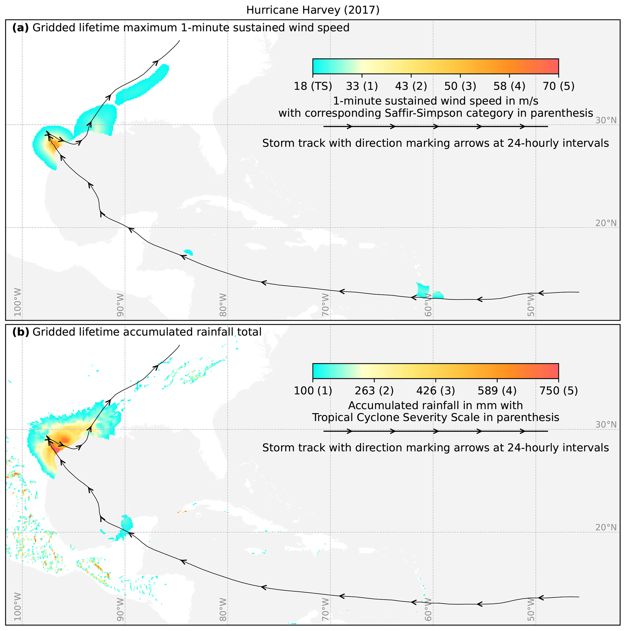
Figure 2Tropical cyclone storm track (a, b, line with arrows), derived maximum wind speeds (a, colored shades), and accumulated rainfall totals (b, colored shades) of Hurricane Harvey that made landfall in Texas (USA) in August 2017. The wind speeds are according to the Holland wind profile (Holland, 1980, 2008), and the rainfall is according to the TCR model (Zhu et al., 2013). The coloring in (b) follows the tropical cyclone severity scale (Bloemendaal et al., 2021).

For surface downwelling longwave radiation (rlds) we follow Fiddes and Gruber (2014) as well as Konzelmann et al. (1994) and account for orographic effects by reducing the clear-sky component of all-sky emissivity with elevation. We assume cloud emissivity remains unchanged when moving from coarse to fine resolution. First, we compute clear-sky emissivity components for both the 0.5^∘ W5E5 grid and the target 30^′′ grid (${\mathit{ϵ}}_{\mathrm{clear}}^{\mathrm{W}\mathrm{5}\mathrm{E}\mathrm{5}}$, ${\mathit{ϵ}}_{\mathrm{clear}}^{\mathrm{highres}}$, respectively):

$$\begin{array}{}\text{(7)}& {\mathit{ϵ}}_{\mathrm{clear}}^{\mathrm{highres}/\mathrm{W}\mathrm{5}\mathrm{E}\mathrm{5}}=\mathrm{0.23}+x\mathrm{1}(p{V}_{\mathrm{dly}}^{\mathrm{highres}/\mathrm{W}\mathrm{5}\mathrm{E}\mathrm{5}}/{\text{tas}}_{\mathrm{dly}}^{\mathrm{highres}/\mathrm{W}\mathrm{5}\mathrm{E}\mathrm{5}}{)}^{\mathrm{1}/x\mathrm{2}},\end{array}$$

where x1=0.43, x2=5.7, and $p{V}_{\mathrm{dly}}^{\mathrm{highres}/\mathrm{W}\mathrm{5}\mathrm{E}\mathrm{5}}$ is water vapor pressure as a function of relative humidity at the respective resolution (see Fiddes and Gruber, 2014). By using 0.5^∘ W5E5 rlds and tas data and inverting the Stefan–Boltzmann equation we obtain all-sky emissivity:

$$\begin{array}{}\text{(8)}& {\mathit{ϵ}}_{\mathrm{allsky}}^{\mathrm{W}\mathrm{5}\mathrm{E}\mathrm{5}}={\text{rlds}}_{\mathrm{dly}}^{\mathrm{W}\mathrm{5}\mathrm{E}\mathrm{5}}/(\mathit{\sigma }\times ({\text{tas}}_{\mathrm{dly}}^{\mathrm{W}\mathrm{5}\mathrm{E}\mathrm{5}}{)}^{\mathrm{4}}),\end{array}$$

with σ being the Stefan–Boltzmann constant ($\mathrm{5.67}\times {\mathrm{10}}^{-\mathrm{8}}$ J s⁻¹ m⁻² K⁻⁴). In a next step, the cloud-based component of emissivity ($\mathrm{\Delta }{\mathit{ϵ}}_{\mathrm{dly}}^{\mathrm{W}\mathrm{5}\mathrm{E}\mathrm{5}}$) can be estimated as the difference between all-sky and clear-sky emissivity, which is then regridded to the target grid via bilinear interpolation.

$$\begin{array}{}\text{(9)}& \mathrm{\Delta }{\mathit{ϵ}}_{\mathrm{dly}}^{\mathrm{W}\mathrm{5}\mathrm{E}\mathrm{5}}={\mathit{ϵ}}_{\mathrm{allsky}}^{\mathrm{W}\mathrm{5}\mathrm{E}\mathrm{5}}-{\mathit{ϵ}}_{\mathrm{clear}}^{\mathrm{W}\mathrm{5}\mathrm{E}\mathrm{5}}\end{array}$$

In a last step we obtain elevation-corrected longwave radiation (rlds_dly) by adding $\mathrm{\Delta }{\mathit{ϵ}}_{\mathrm{dly}}^{\mathrm{W}\mathrm{5}\mathrm{E}\mathrm{5}}$ to the high-resolution clear-sky emissivity (${\mathit{ϵ}}_{\mathrm{clear}}^{\mathrm{highres}}$) and applying the Stefan–Boltzmann law again:

$$\begin{array}{}\text{(10)}& {\text{rlds}}_{\mathrm{dly}}=({\mathit{ϵ}}_{\mathrm{clear}}^{\mathrm{highres}}+\mathrm{\Delta }{\mathit{ϵ}}_{\mathrm{dly}}^{\mathrm{W}\mathrm{5}\mathrm{E}\mathrm{5}})\times \mathit{\sigma }\times ({\text{tas}}_{\mathrm{dly}}^{\mathrm{highres}}{)}^{\mathrm{4}}.\end{array}$$

As soon as the CHELSA approach is extended to also cover the missing variable we plan to provide these data and test the sensitivity of the impact simulations to these two alternative downscaling methods.

3.1.3 Default counterfactual data

To simulate the baseline no-climate-change state of a human or natural system that is required for impact attribution, we provide a detrended version of the observational factual forcing data using the ATTRICI approach (ATTRIbuting Climate Impacts, Mengel et al., 2021). The method identifies the long-term shifts in the factual daily climate variables that are correlated with global mean temperature change assuming a smooth annual cycle of the associated scaling coefficients for each day of the year. The observed trends since 1901 are then removed from the observational data by projecting the observed data onto the estimated distributions assuming a fixed 1901 level of global warming. The projection is done through quantile mapping, a method borrowed from the bias adjustment literature. In this way we preserve the internal variability of the observed data in the sense that factual and counterfactual data for a given day have the same rank in their respective statistical distributions. The impact model simulations forced by the counterfactual climate inputs therefore allow for quantifying the contribution of the observed climate change (no matter from where the trends originate) to observed long-term changes in impact indicators but also for quantifying the contribution of the observed trend in climate to the magnitude of individual impact events.

Table 6Tropical cyclone information provided as part of the ISIMIP3a climate-related forcing.

Download XLSX

3.2 Tropical cyclone (TC) data (factual)

As additional CRF, we provide historical TC tracks (information about the observed location of minimal pressure), with associated gridded wind and rain fields (see variable names and units in Table 6 and the maps of maximum wind speed and accumulated rainfall totals for the example of Hurricane Harvey in Fig. 2). In addition to this purely climate-related forcing, we also provide wind exposure in terms of (i) shares of national territory affected by extreme winds speeds, (ii) national shares of people exposed to extreme winds speeds, and (iii) national shares of economic assets affected by extreme winds speeds as derived from the estimated wind fields and historical population and GDP distributions (see below). Table 6 provides a comprehensive list of all variables, with their meaning and resolution as well as their source.

TC tracks include the position of storm center, central pressure, environmental pressure, radius of maximum wind speed, and the outermost closed isobar. We provide processed track information of historical TCs from 1950 to 2021. The information is derived from IBTrACS, the most comprehensive global dataset of historical TC activity (Knapp et al., 2010) that provides information about the location of the storm center, the pressure at the center and at the outermost closed isobar, and the maximum 1 min sustained wind speed as reported by the WMO Regional Specialized Meteorological Centers (RSMCs) and by agencies in Shanghai and Hong Kong. For recent events and most reporting agencies, IBTrACS also contains observational information about the radius from the center where maximum wind speed is attained and the radius of the outermost closed isobar. Information is provided in at least 6-hourly time steps. Usually temporal resolution reaches 3 h or even less. The latest version (v04r00) of IBTrACS is continuously updated with near-real-time data taken from regional meteorological agencies. The data are marked as provisional before they are replaced by the so-called best track data up to 2 years after the events. IBTrACS contains data from 1842 to present, but coverage by the WMO RSMCs starts much later for some of the basins (around 1850 for the North Atlantic and southern Indian Ocean, in 1905 for the South Pacific, in 1950 for the North Pacific, and in 1990 for the northern Indian basin). Data quality is globally consistent starting from the mid-1970s when satellite observations became available.

The dataset we provide uses best track data from 1950 to 2021. For each TC in IBTrACS, we merge the data of different reporting agencies into a single track dataset with information about the following variables: time, location of the storm center, ocean basin, central pressure, maximum 1 min sustained wind speed, environmental pressure, radius of maximum wind speeds, and radius of the outermost closed isobar (see Table 8). Several processing steps are applied to ensure consistency and completeness of the data. For each storm, the variables that are not reported by the officially responsible WMO RSMC for this storm are taken from the next agency in the following list that did report this variable for this storm: the US agencies (NHC, JTWC, CPHC), Japanese Meteorological Agency, Indian Meteorological Department, MeteoFrance (La Réunion), Bureau of Meteorology (Australia), Fiji Meteorological Service, New Zealand MetService, Chinese Meteorological Administration, and Hong Kong Observatory. Thus, for different storms, the same variable might be taken from different agencies. As sustained wind speeds are reported at different averaging intervals by different agencies, we use multiplicative factors to rescale all wind speeds to 1 min sustained winds (Knapp and Kruk, 2010). All variables are extracted at the highest temporal resolution where time and location information is available in IBTrACS. Temporal reporting gaps within a variable are linearly interpolated so that the temporal resolution is at least 3-hourly. After interpolation, time steps where neither central pressure nor maximum wind speeds are available are discarded. Tracks with fewer than two valid time steps are discarded. If at least central pressure or maximum wind speed is available, one variable is estimated from the other using statistical wind–pressure relationships. Missing RMW and ROCI values are estimated from the central pressure using statistical relationships. Finally, missing environmental pressure values are filled with basin-specific defaults (1010 hPa for the Atlantic and eastern Pacific, 1005 hPa for the Indian Ocean and western Pacific, and 1004 hPa for the South Pacific).

We provide two additional along-track variables that are taken from the European Reanalysis (ERA5; Hersbach et al., 2020) and that are needed for the computation of precipitation (see below): the temperature at the storm center on the 600 hPa pressure level and the wind speed on the 850 hPa pressure level averaged over the 200–500 km annulus around the storm center.

For gridded maps of (maximum) wind speeds, we derive two different gridded wind field products from an extrapolation of the observed TC track information to gridded estimates of surface wind speeds (1 min sustained winds at 10 m above ground) at a spatial resolution of 300 arcsec (approximately 10 km). The two products are based on circular wind fields from different radial wind profiles. The first is a semiempirical model that estimates the full wind profile from the central pressure variable based on the gradient wind balance assumption (Holland, 1980, 2008). The second more physics-based model uses the less reliable maximum wind speed variable to derive the wind profile from the boundary layer angular momentum balance (Emanuel and Rotunno, 2011). This wind profile represents the storm's inner core very well but tails off too sharply in the outer region (Chavas and Lin, 2016). However, for high-impact events, the core is the most relevant storm region, and outer wind profiles are not analytically solvable, incurring considerable computational expense when applied to a large track set.

In both cases, the circular wind fields are combined with translational wind vectors that arise from the TC movement, assuming that the influence of translational wind decreases with distance from the TC center (Cyclone Database Manager, 2023). We use the highest available temporal resolution (up to 3-hourly) provided in IBTrACS and interpolate it to 1-hourly resolution before applying the parametric wind field models. In a post-processing step, we also calculate the maximum value of wind speeds over the duration of the TC event (max_wind).

The approach by Holland has been successfully applied in socioeconomic risk and impact analyses (Peduzzi et al., 2012; Geiger et al., 2018; Eberenz et al., 2021). The Emanuel–Rotunno approach has been used for storm surge simulations (Krien et al., 2017; Marsooli et al., 2019; Gori et al., 2020; Yang et al., 2021) and as the basis for the rain field model that we describe below (Feldmann et al., 2019).

In terms of wind exposure, as an extension of the tropical cyclone exposure dataset TCE-DAT (Geiger et al., 2018), we provide national shares of people and economic assets exposed to 1 min sustained winds above 34, 48, 64, and 96 kt for each storm. In addition to that, shares of national territory affected by 1 min sustained winds above 34, 48, 64, and 96 kt are provided. To estimate the exposed population and assets we use the histsoc population and GDP distributions described in Sect. 4.1 and 4.2, respectively. The GDP values are converted to assets by applying the decadal (2010–2019) mean of national capital stock to GDP ratios from the Penn World Table version 10.0 (Feenstra et al., 2015). We also provide exposed population and assets assuming fixed 2015 population and asset distributions.

For precipitation, we are also planning to provide rainfall fields, following a physics-based model that simulates convective TC rainfall by relating the precipitation rate to the total upward velocity within the TC vortex (Zhu et al., 2013). The approach has been successfully applied in rainfall risk assessments in the US (Feldmann et al., 2019; Gori et al., 2022). The rain rate will be simulated for all events in the IBTrACS database at 0.5-hourly temporal and 300 arcsec (approximately 10 km) spatial resolution within a 1500 km radius around the storm center. We provide the derived rainfall totals at hourly resolution as well as the maximum 24-hourly rainfall total during the entire storm duration since this variable is frequently used for rainfall risk assessment studies (Fagnant et al., 2020).

Different TC wind profiles can be used as an input for the rain field model (Lu et al., 2018; Xi et al., 2020). We will provide the rainfall fields for the two wind profile models by Holland and Emanuel–Rotunno that we also use for the wind fields described above.

Figure 3Observed and reconstructed coastal relative water levels at New York, USA. The counterfactual baseline represents water levels without long-term trend since 1900. Water levels are aggregated to monthly means in panel (a) and daily means in the year 2011 in panel (b), while panel (c) shows some of the data at hourly resolution. The reconstructed water levels are available as monthly mean values from 1901 to 1978 and as hourly mean values from 1979 to 2015.

Download

Table 7Information about coastal water levels provided as ISIMIP3a climate-related forcing.

Download Print Version | Download XLSX

3.3 Coastal water levels (factual + counterfactual)

To enable the quantification of impacts of historical relative sea level rise on coastal systems we provide observation-based coastal water levels building on the HCC dataset (hourly coastal water levels with counterfactual; Treu et al., 2023). In contrast to absolute sea levels, relative sea levels are measured against a land-based reference frame (tide gauge measurements). This means that they are determined not only by thermal expansion, loss of land ice, or dynamical processes influenced by climate change, but also by vertical land movements (Wöppelmann and Marcos, 2016) induced by, e.g., glacial isostatic adjustments (Caron et al., 2018; Whitehouse, 2018) or human interventions such as groundwater abstraction (Wada et al., 2016b). HCC encompasses factual and counterfactual coastal water levels along global coastlines from 1901 to 1978 at monthly resolution and from 1979 to 2015 at hourly resolution (see Fig. 3). The counterfactual coastal water levels are derived from the factual dataset by removing the trend in relative sea level since 1900. The detrending preserves the timing of historical extreme sea level events similar to the counterfactual atmospheric climate forcing described in Sect. 3.1 (see Fig. 3b). Hence, the data can be used for an event-based attribution of, e.g., observed flooding to observed relative sea level rise with pairs of impact simulations driven with the factual and counterfactual datasets. It is important to highlight that “attribution to observed changes in relative water levels” does not imply attribution to anthropogenic climate forcing because such observed changes may include trends that are not driven by human greenhouse gas emissions. Important sources for such trends are the ongoing adjustments of ice sheets, glaciers, and the Earth's crust to climate conditions before industrialization (Slangen et al., 2016) and the land subsidence due to water, gas, and oil extraction (Nicholls et al., 2021). In the following the derivation of the data is described in more detail.

Default factual data. To capture the impacts of extreme water levels we provide hourly observation-based coastal water levels as forcing data. To this end we combine the Coastal Dataset for the Evaluation of Climate Impact (CoDEC) dataset (Muis et al., 2020) that describes high-frequency variation of sea level along global coastlines with a recent reconstruction of observed long-term sea level rise (Dangendorf et al., 2019). The CoDEC hourly data build on a shallow-water model with fixed ocean density driven by ERA5 wind and atmospheric pressure fields. The CoDEC data thus start only in the year 1979 and do not include variations due to ocean density changes and multiyear trends from observed sea level rise or vertical land movement. In contrast, the hybrid reconstruction (HR) dataset from Dangendorf et al. (2019) represents sea level change since 1900 on a monthly timescale, including density variations and multiyear trends. Long-term sea level change in HR is based on fitting theoretically known and modeled spatial–temporal fields of individual contributing factors of sea level change to a set of observations of sea level change from tide gauges. The individual contributing factors are theoretically known cryospheric fingerprints from two ice sheets, 18 major glacier regions, glacial isostatic adjustment from 161 Earth rheological models, and dynamic changes in sea surface height modeled by six global climate models. Short-term sea level variations are represented in HR by extending the spatiotemporal patterns from satellite altimetry back to the year 1900 using tide gauge records. We create the HCC dataset by low-pass-filtering the HR dataset and high-pass-filtering the CoDEC dataset before summing them. Vertical land motion is subsequently added to yield relative changes in water levels along global coastlines. HCC shows improved agreement with tide gauge records on hourly to monthly timescales when compared to CoDEC due to the inclusion of density variations. This is most apparent for lower latitudes. The performance on inter-annual timescales is equal to Dangendorf et al. (2019).

Default counterfactual data. To estimate the effects of historical sea level rise on coastal systems, we provide a counterfactual sea level dataset as forcing for coastal impact models (Treu et al., 2023). To this end the long-term trend in the HCC data (1900–2015) was identified by a simple quadratic model in time and subtracted from the factual HCC data. The quadratic model assumes a constant acceleration of sea level rise over time. Analysis of sea level rise acceleration shows variation throughout the last century with an acceleration phase in the early century followed by a deceleration and then again acceleration until today (Dangendorf et al., 2019). By design, this variation is not included in our quadratic trend estimate. In general, we expect our trend estimation to largely exclude natural variability from the trend due to the low dimensionality of the trend model and the long data period. This is a desired outcome and preserves the natural variability in the counterfactual. Extreme sea level events have the same timing in the counterfactual and the factual dataset, facilitating event-based impact attribution.

3.4 Ocean data (factual)

Default factual data. For the fisheries and marine ecosystem models, we provide a number of physical and biogeochemical variables for the period 1961 to 2010 at different depth levels in the ocean (see Table 8). Since direct measurements of these variables are very scarce (Sarmiento and Gruber, 2006; WOCE Atlas, 2023), the only way to obtain a globally (or even regionally) complete and consistent forcing dataset is to use numerical models. Global ocean models, which also serve as oceanic components of Earth system models, often simulate many or all of the required variables. To let observations at least indirectly enter the oceanic forcing data for ISIMIP3a, we provide outputs from an ocean model run that is forced by an observation-based reanalysis product of atmospheric forcing (Liu et al., 2021). Compared to the oceanic forcing (Stock et al., 2014) provided to generate the ISIMIP2a simulations for the marine ecosystems and fisheries sector (Tittensor et al., 2018), this new dataset is based on the latest GFDL-MOM6 and COBALTv2 physical and biogeochemical ocean models running on a tripolar 0.25^∘ grid and using the JRA-55 reanalysis (Tsujino et al., 2018) as the surface forcing, in contrast to the inter-annual forcing dataset of Large and Yeager (2009), which was previously used to drive GFDL-MOM4. The simulations also account for dynamic, time-varying river freshwater and nitrogen inputs that were simulated based on GFDL's land–watershed model LM3-TAN (Land Model version 3 with Terrestrial and Aquatic Nitrogen; Lee et al., 2019), adjusted using observations from the Global Nutrient Export from WaterSheds (NEWS) database (Seitzinger et al., 2006). To create the default obsclim climate-related forcings for the fisheries and marine ecosystem models these ocean model simulation data have been interpolated to a regular 0.25^∘ grid while vertical resolution is preserved. In contrast to the atmospheric data, oceanic CRFs are provided at monthly temporal resolution.

Low-resolution factual data. To test to what degree a lower spatial resolution of the climate-related forcings affects the impact model simulations, the oceanic climate-related forcings have also been aggregated to 1^∘ resolution as input for the “obsclim + histsoc, 60arcmin” sensitivity experiment.

CRF for the 1955-riverine-input sensitivity experiment. The 1955-riverine-input sensitivity experiment builds on the 0.25^∘ GFDL-COBALT2 simulation forced by the JRA-55 reanalysis but without time-varying riverine inputs. Instead the influxes of freshwater and nutrients are fixed at mean 1951 to 1958 levels as described in the “control run” introduced by Liu et al. (2021). The data are interpolated to a regular 0.25^∘ grid in the same way as the default obsclim CRFs.

We currently do not provide counterfactual versions of the ocean data forcing, though options are being explored.

Table 8ISIMIP3a oceanic climate-related forcing. Variables with suffixes -bot, -surf, and -vint were obtained from the seafloor, the top layer of the ocean, and vertical integration, respectively.

Download XLSX

Figure 4Historical evaluation of population for different continents. Total number of people living in the region (a) and the urban population as a fraction of the total population per region (b).

Table 9Population data provided as part of the ISIMIP3a direct human forcing.

Download Print Version | Download XLSX

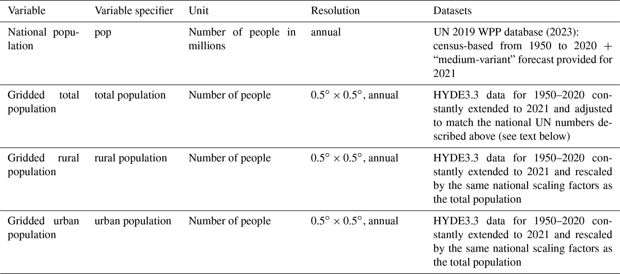
4.1 Population data

For ISIMIP3a we provide consistent gridded and national population data (see Table 9) by rescaling the gridded data to match the national aggregates. Figure 4 shows the temporal evolution of total and urban population for different continents.

National data. Annual national population data are taken from the 2019 UN World Population Prospects (WPP) database for the period from 1950–2021 (United Nations, 2019). The 2019 revision of the WPP provides census-based population numbers from 1950 through 2020. For the year 2021, we use the “medium variant” of the probabilistic forecast also provided by the WPP. The forecast accounts for the past experience of each country, while reflecting uncertainty about future changes based on the past experience of other countries under similar conditions (see United Nations, 2019, for details). For countries not covered in the database, estimates are taken from the MissingIslands dataset (Arujo et al., 2021) to finally provide population data for 249 countries.

Gridded data. We provide gridded population data that are based on HYDE v3.3 (Kees Klein Goldewijk, personal communication, 2022). Just like the original dataset we provide total, rural, and urban population per grid cell. The original HYDE 3.3 data were on a $\mathrm{1}/\mathrm{12}$^∘ × $\mathrm{1}/\mathrm{12}$^∘ grid and have been interpolated to ISIMIP's 0.5^∘ × 0.5^∘ grid. Furthermore, the land–sea distinction was modified to comply with the ISIMIP country mask (see Table 1). Before the year 1950 HYDE provides data every 10 years, and the intermediate years have been filled by linear interpolation. Also, the original HYDE data end in 2020. So to cover the whole ISIMIP3a time frame the final year 2020 has been duplicated as 2021. In this way annual coverage for 1850 to 2021 has been achieved.

Data for all grid cells of a country, as defined by the ISIMIP 0.5^∘ × 0.5^∘ fractional country map (see Table 1), have been rescaled such that the country's total population matches the numbers provided in the national population data. Since the national data only start in 1950, all years prior to 1950 have been rescaled by the national scaling factors of 1950. The urban and rural populations have been rescaled by the same national scaling factors as the total population.

Figure 5Aggregated GDP (Int$ PPP 2005) for different continents.

Table 10GDP data provided as part of the ISIMIP3a direct human forcing.

Download Print Version | Download XLSX

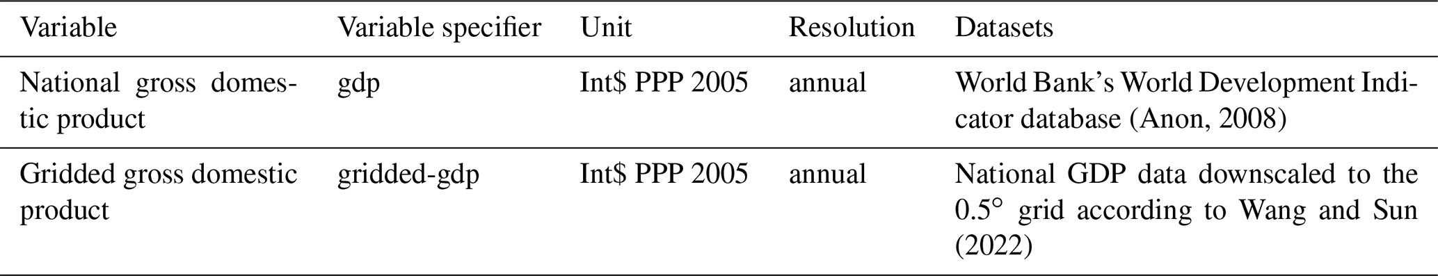
4.2 Gross domestic product (GDP)

Similar to the population data we also provide gridded and national GDP data (see Table 10). The downscaling of the national numbers is based on population and nightlight data (see below). In contrast to ISIMIP2a the gridded GDP and population data are now consistent such that previous artifacts in the derived GDP per capita could be eliminated (see below). Figure 5 shows the historical increase in GDP for different continents.

National GDP data. Time series of per capita GDP for the time period 1960–2021 are taken from the World Bank's World Development Indicator database (WDI) (Anon, 2008) and converted into constant 2005 Int$PPP using deflators and PPP conversion factors from WDI. For countries not covered in the WDI database, data from the MissingIslands dataset (Arujo et al., 2021) are used to allow covering 249 countries. Following a method developed by Koch and Leimbach (2023), the values for the year 2021 are derived from the IMF's World Economic Outlook short-term estimates of GDP per capita growth (International Monetary Fund, 2021) that comprise estimates of the growth impacts of the Covid-19 shock.

Gridded GDP data. Gridded GDP data at 0.5^∘ resolution are derived from the national GDP time series by applying the LitPop method (Zhao et al., 2017; Eberenz et al., 2019), which uses the ISIMIP3a gridded population based on HYDE v.3.3 and nighttime light (NTL) data to downscale national GDP data for the period 1960–2021 to the ISIMIP 0.5^∘ × 0.5^∘ grid.

As the disaggregation of GDP is not only based on population but also uses the NTL GDP per capita, it is not constant within different countries. Deriving the gridded GDP data from the gridded population data provided within ISIMIP3a ensures that the both datasets can be combined such that the associated GDP per capita no longer shows the artifacts that have been found in the ISIMIP2a GDP per capita (ISIMIP2a, 2023).

Figure 6Share of global land area excluding Antarctica covered by rainfed cropland (green), irrigated cropland (blue), and pasture (orange) [%]. The information is from the LUH v2 dataset provided as direct human forcing for ISIMIP3a (see details below).

Download

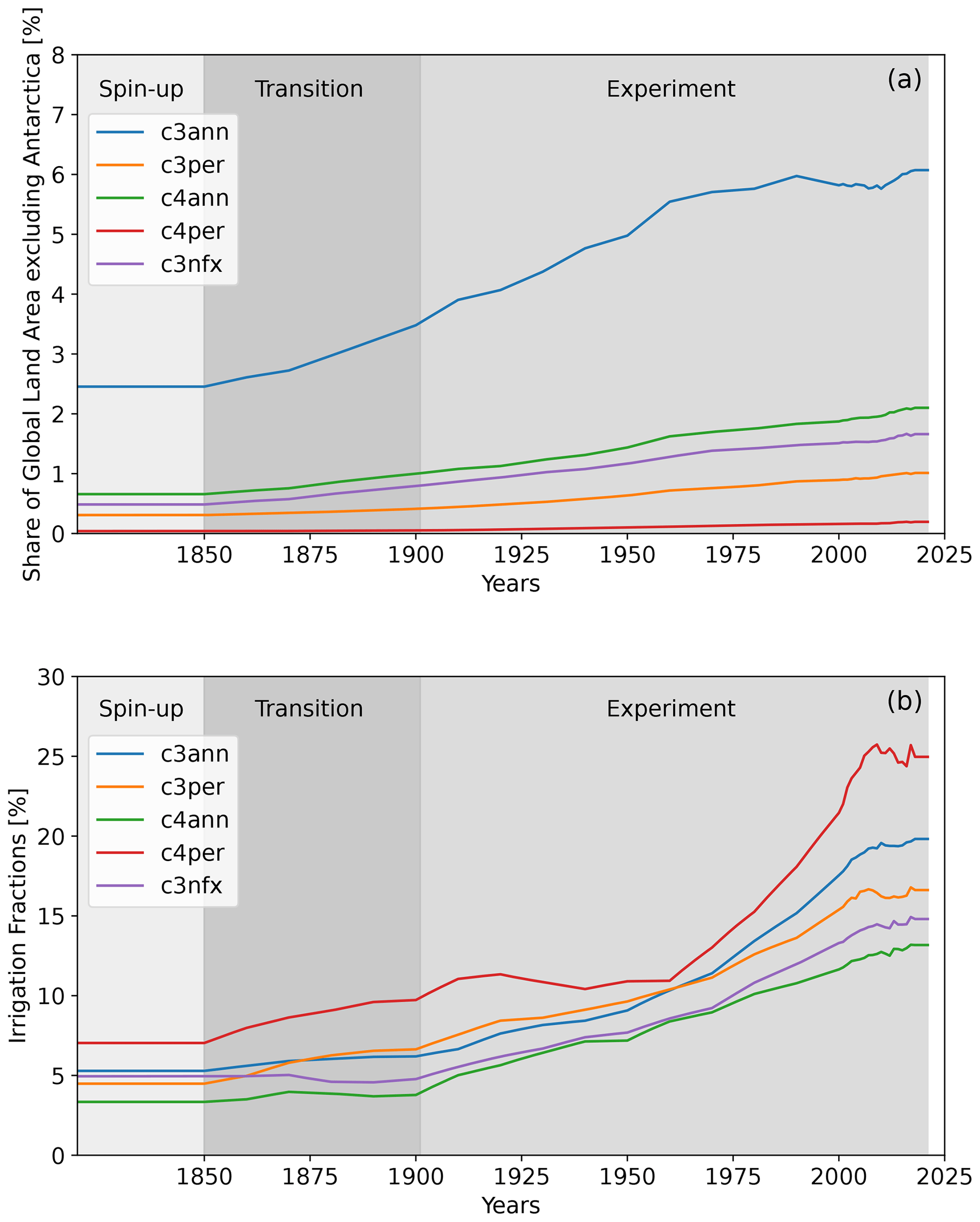
Figure 7(a) Share of global land area excluding Antarctica covered by different groups of crops (C₃ annual – blue, C₃ perennial – orange, C₄ annual – green, C₄ perennial – red, C₃ nitrogen-fixing – purple). (b) Fraction of irrigated land for the different groups of crops. The information is from the LUH v2 dataset (see details on further disaggregation of the LUH v2 groups below).

Download

Table 11Historical land use and irrigation patterns provided as part of the ISIMIP3a direct human forcing.

Download XLSX

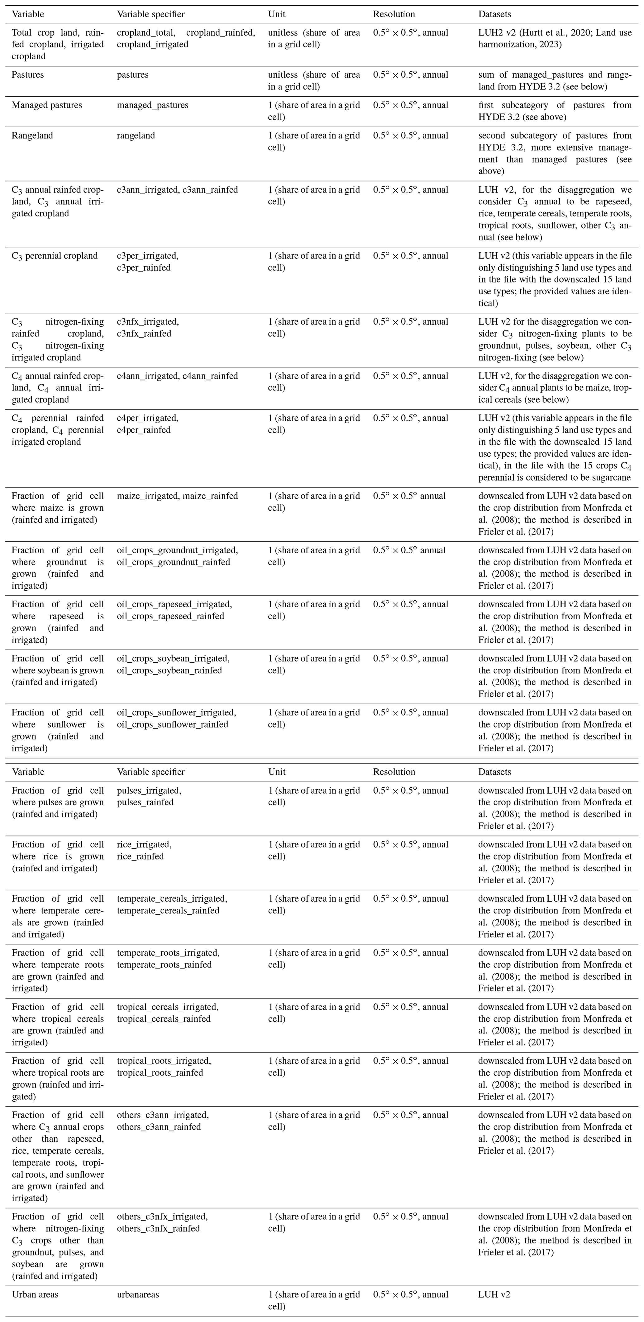
4.3 Land use and irrigation patterns

Historical land use and irrigation patterns for ISIMIP3a simulations are taken from LUH v2 (Hurtt et al., 2020; Land use harmonization, 2023). The dataset is, up to 2018, identical to the data provided with ISIMIP2b. The data are based on the HYDE 3.2 land use dataset (Klein Goldewijk et al., 2017) and have been constantly extended up to 2021, i.e., by copying the 2018 patterns into 2019, 2020, and 2021.

The original HYDE 3.2 data distinguish four categories of land use: rainfed and irrigated cropland, managed pastures, and more extensively managed rangelands (see Table 11). The latter two categories are combined into grazing lands (ISIMIP variable pastures, see Fig. 6). In LUH v2 the crop land information is further downscaled to five crop types: C₃ annual plants, C₃ perennial plants, C₃ nitrogen-fixing plants, C₄ annual plants, and C₄ perennial plants (see global aggregates in Fig. 7). In the same vein as the HYDE case, the LUH v2 dataset distinguishes between rainfed and irrigated croplands. For the purpose of driving the ISIMIP impact models, the LUH v2 data were interpolated from the original 0.25^∘ × 0.25^∘ to the standard ISIMIP 0.5^∘ × 0.5^∘ global grid. In a further downscaling step the land use data for five crops have been downscaled even further to 15 crop types (see global aggregates in Fig. 7). For this purpose the Monfreda land use dataset (Monfreda et al., 2008) has been used. It describes the crop land areas of 175 crops in the year 2000, and we use this to downscale the five crop categories into land use areas of 15 more specific crop types (maize, groundnut, rapeseed, soybeans, sunflower, rice, sugarcane, pulses, temperate cereals including wheat, temperate roots, tropical cereals, tropical roots, other annual, other perennial, and other N-fixing). The ratios determined from the year 2000 numbers have then been applied to all years. For further details please refer to Frieler et al. (2017).

The area outside of the specified agricultural and urban land is considered “natural vegetation” and not prescribed further to not constrain the dynamical vegetation models.

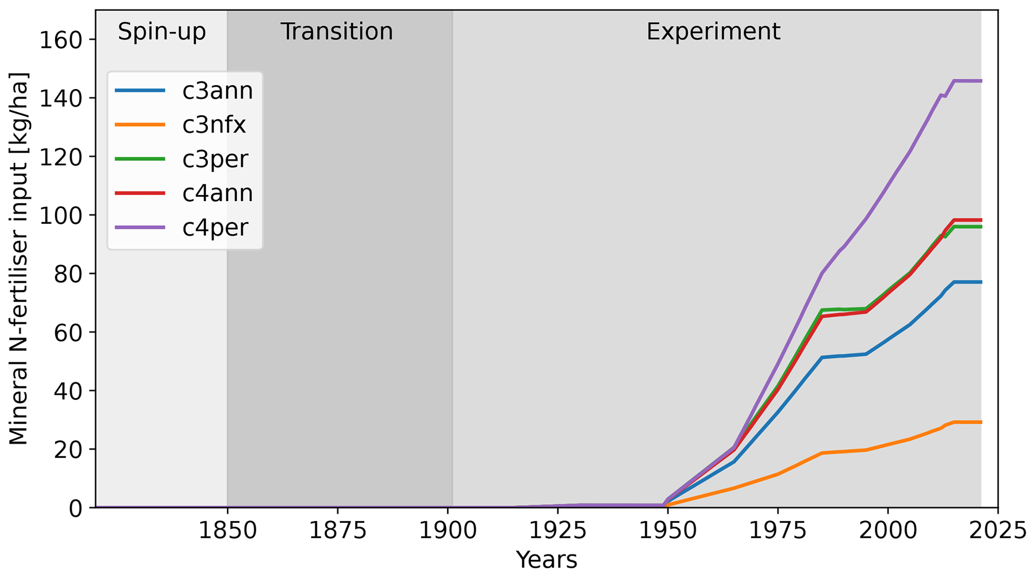
Figure 8Mean mineral N-fertilizer input averaged across the land areas where the considered crop groups are grown.

Download

Table 12Fertilizer inputs provided as part of the ISIMIP3a direct human forcing.

Download Print Version | Download XLSX

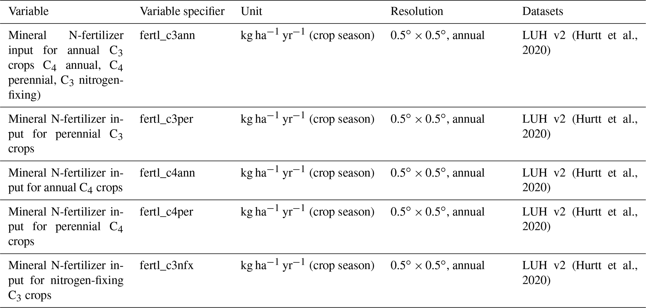
4.4 Fertilizer input

The LUH v2 dataset also includes national application rates of industrial nitrogen fertilizer (Hurtt et al., 2020). This does not include manure. The fertilizer data are not based on HYDE but were derived from other sources. The data for the years 1915–1960 are based on Smil (2001); those for 1961–2011 are based on a compilation by Zhang et al. (2015), which in turn is based on FAOSTAT (FAO, 2016), and data for 2012–2015 are based on a projection by the International Fertilizer Association (IFASTAT, 2015). For the pure crop runs within ISIMIP, where the considered crops are assumed to be grown everywhere without a land use specification, the LUH v2 national fertilizer inputs are assumed to be applied everywhere within the country. To calculate crop production, the LUH2 v2 land use patterns are applied in post-processing, i.e., by multiplying the crop yields from the pure crop run with the land use patterns (fraction of the grid cell where the crop has been grown).

Table 13Land transformation and wood harvest provided as part of the ISIMIP3a direct human forcing.

Download XLSX

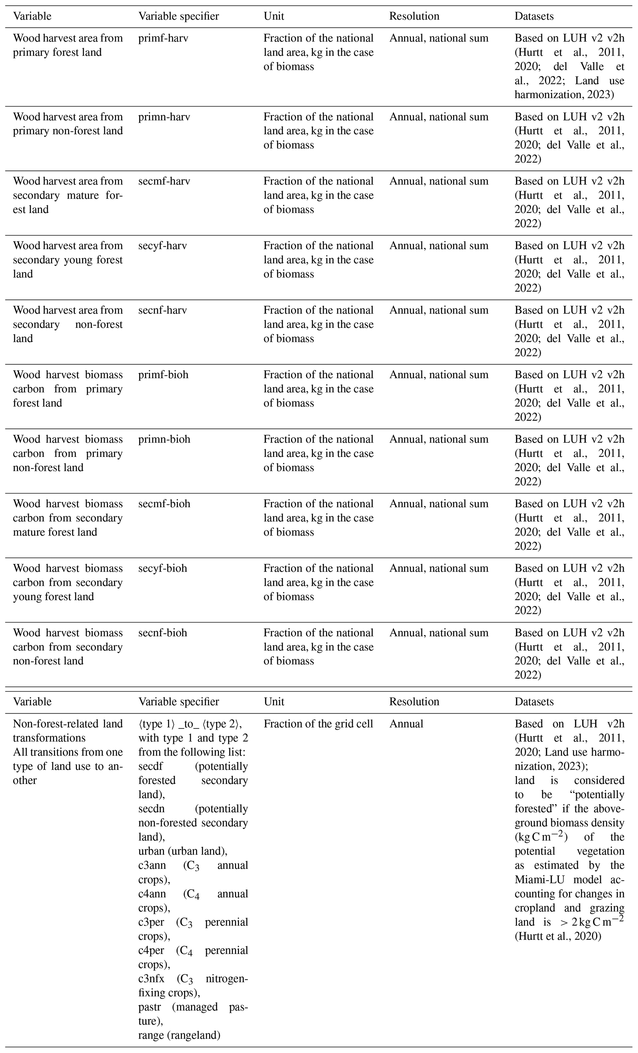
4.5 Land transformation

These datasets are based on the LUH v2 Harmonization Data Set covering 850 to 2015 (Hurtt et al., 2020; Land use harmonization, 2023). The wood harvest data were obtained by aggregating from the original LUH v2 grid to the ISIMIP 0.5^∘ × 0.5^∘ grid (first-order conservative remapping) and then aggregating to the national sums. Wood harvesting data are used in the vegetation models to mimic wood removal as part of forest management and clearing and have a strong influence on the carbon balance. National data are provided so that models can use their internal routines to distribute the harvesting within a country's forest area. The gridded land transformation data were obtained by aggregating from the original LUH v2 grid to the ISIMIP 0.5^∘ × 0.5^∘ grid; these data always end a year earlier than all other land use data because a year in these datasets actually describes the changes from the current to the next year. The data have been extended up to 2021 by copying the 2015 data into the following years (files end in 2020).

Table 14Nitrogen deposition provided as part of the ISIMIP3a direct human forcing.

Download Print Version | Download XLSX

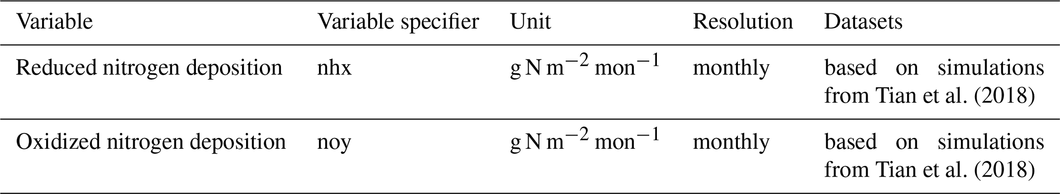
4.6 Nitrogen deposition

Reduced nitrogen deposition and oxidized nitrogen deposition (NH_x, NO_y) are based on simulations by the NCAR Chemistry–Climate Model Initiative during 1850–2014 (Tian et al., 2018). Nitrogen deposition data were interpolated to 0.5^∘ by 0.5^∘ using the nearest grid point method. Data in 2015–2021 are assumed to be the same as those in 2014.

Table 15Crop calendar provided as an optional representation of agricultural management. The information is given for 18 crop types.

Download Print Version | Download XLSX

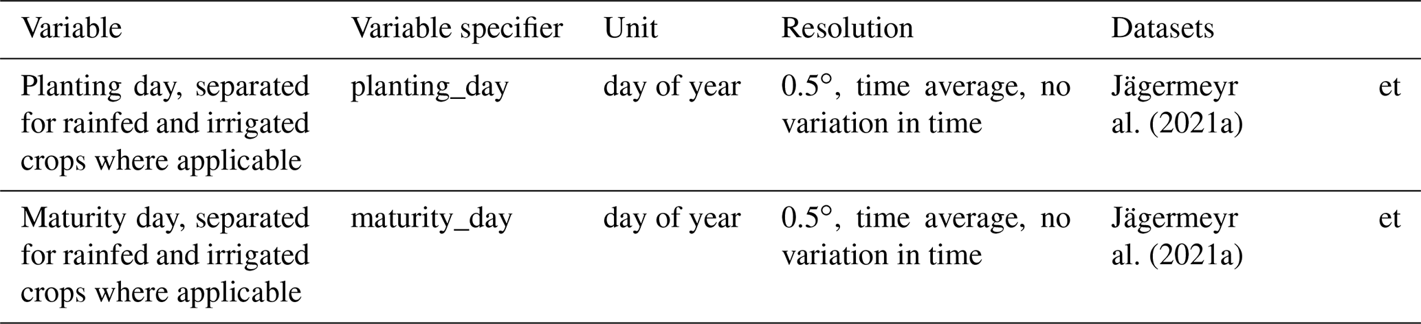
4.7 Crop calendar

Unfortunately, there is no global dataset describing changes in growing seasons across the historical period. Instead we provide a static crop calendar that has been developed within the AgMIP Global Gridded Crop Model Intercomparison GGCMI and merges information from various observational data sources (Jägermeyr et al., 2021a). It provides planting and maturity days for 18 different crops on the ISIMIP standard 0.5^∘ grid. Grid cells outside of currently cultivated areas are spatially extrapolated (details below). For wheat and rice two growing seasons are provided, while for all other crops the calendar only specifies one main growing season. The reported growing seasons should not be considered the growing seasons for one specific year but as “representative growing season” across recent years. Within the crop models different crop varieties are represented by different heat units required to reach physiological maturity. The crop calendar should be implemented by adjusting the required heat units to the average of the annual sums of heat units between the specified planting and maturity date over all growing seasons between 1979 and 2010.

If modelers use a temporal adjustment of cultivars by varying required heat units in response to socioeconomic development or historical climate change this is certainly allowed within the histsoc setup. If cultivars are fixed according to the method described above this simulation will be considered a 2015soc simulation as long as other direct human drivers are also held constant at 2015 levels. However, if, e.g., fertilizer inputs are varied over time according to provided forcing data (see Sect. 4.4), the run will be considered a histsoc run.

GGCMI is currently working on a temporally resolved global crop calendar at the same spatial resolution based on various new data sources including agricultural ministries, census reports, phenological data bases, and experimental sites. This dataset will be published separately and could then be used to inform histsoc simulations.

Table 16Information about dams and reservoirs.

Download XLSX

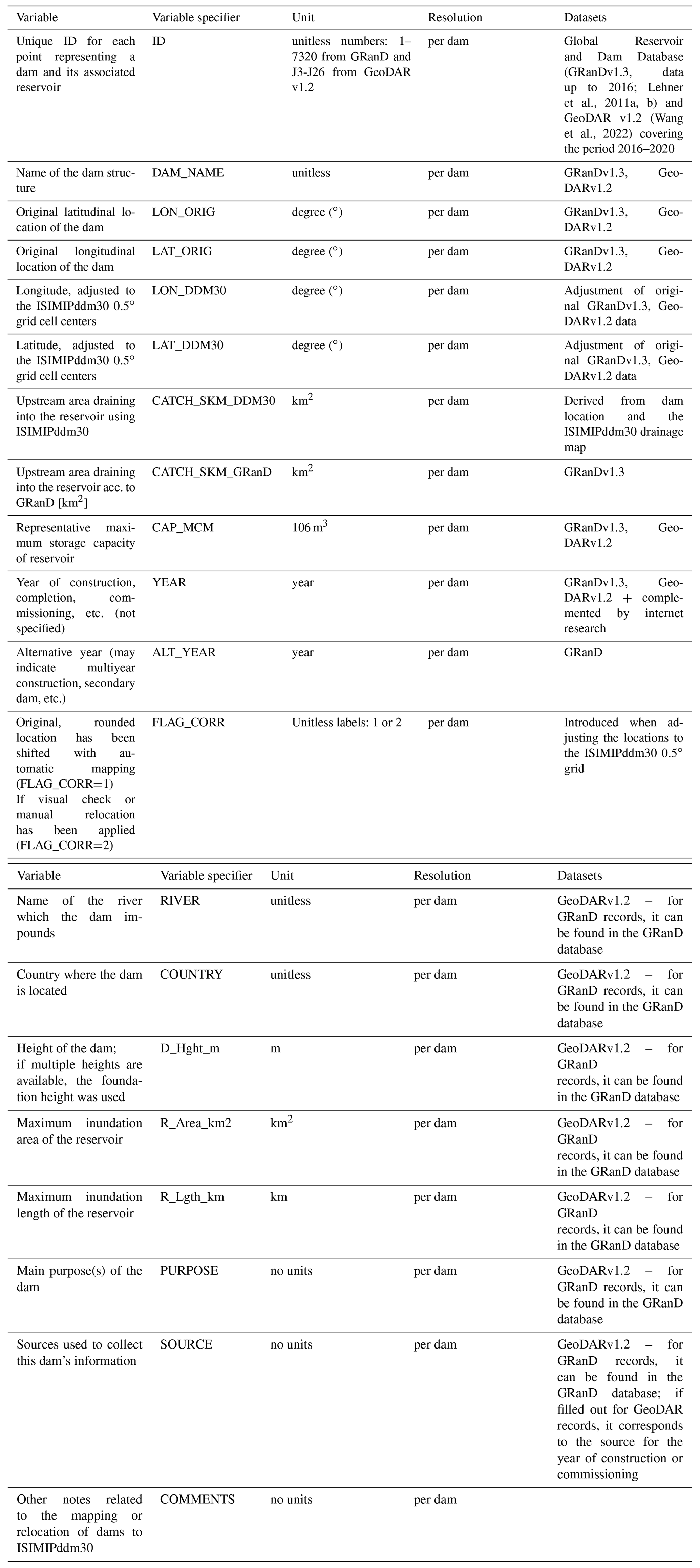
4.8 Dams and reservoirs

In order to offer a consistent and common source of information about reservoirs and associated dams for climate impact modelers (see Table 16), we joined the Global Reservoir and Dam Database of the Global Water System Project (GRanD v1.3; (Lehner et al., 2011a, b) with a subset of the Georeferenced global Dams And Reservoirs (GeoDAR v1.2) database (Wang et al., 2022), developed at Kansas State University (KSU) and provided by Jida Wang ahead of publication, so that it could be provided when launching ISIMIP3 in 2020. These additional dams have construction or projected finalization dates between 2016 and 2025, while GRanD v1.3 includes dams constructed up until 2017. In total, the combined database now includes 7331 dams whose construction will be finished by 2025. It includes dams that were constructed before the simulation period but still exist (the first reported dam was finished in the year 286). For the simulations described here, dams with (projected) construction dates after 2020 are not considered; these will become relevant in the ISIMIP3b simulations, with the exception of the Grand Ethiopian Renaissance Dam, which we decided to include since its reservoir reached the first stage of filling of 4.9 km³ in July 2020 (BBC news: Nile dam row, 2020; Tractebel, 2020).

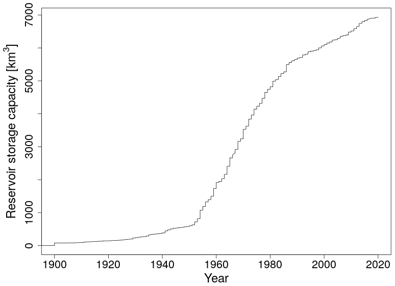
Figure 9Cumulative reservoir storage capacity between 1900 and 2020. Reservoirs that were active before the year 1901 have been assigned to the year 1900. The horizontal axis shows the year of construction, completion, or commissioning, reflecting ambiguity in available data.

Download

The original GRanDv1.3 dam locations were mapped to the global 30 min drainage direction map (ISIMIPddm30, (Müller Schmied, 2022) based on DDM30 (Döll and Lehner, 2002) by applying the following algorithm.

Firstly, the locations have been rounded to the closest 0.5^∘ grid cell center. Then, the area of the upstream catchment draining into the GRanD reservoirs (previous version of GRanDv1.3) in the ISIMIPddm30 map has been calculated and compared against the ones reported in GRanD. All dams with an upstream area bigger than 10 000 km² in GRanD and more than 50 % deviation from the GRanD upstream area have been shifted to the eight possible neighboring cells. If any of these shifts resulted in a smaller deviation from the GRanD upstream areas, the dam was moved to the grid cell resulting in the smallest deviation in the upstream area.

Additionally, a visual validation and, where appropriate, manual relocation were applied with the aim of finding the best-fitting grid cell from a hydrological perspective. Due to the low resolution of the model grid, reservoirs might get wrongly assigned to, e.g., the main stream (either before or after the confluence of two rivers), even though the dam is located in a particular tributary according to the database.

In those cases, and based on visual GIS inspection, the best location was searched, e.g., by moving the dam location one cell upstream to preserve the routing order and to avoid a different or highly deviating river basin in the ISIMIPddm30 stream network. In the case that a dam is not assigned to any river basin in the ISIMIPddm30 (which can happen due to the difference in spatial resolution), the most suitable location according to the observed upstream area was selected. Because of limited capacity, this visual validation procedure was applied only for dams present in the earlier GranDv1.1 version that have a maximum storage capacity greater than 0.5 km³ (1108 dams), as well as for all 458 additional dams in GRanDv1.3 and the 11 dams (excluding post-2020 dams) added from GeoDAR v1.2 but not for several thousand smaller dams present in GranDv1.1. In total the reported dams have a global cumulative storage capacity of approximately 6932 km³ (Fig. 9).

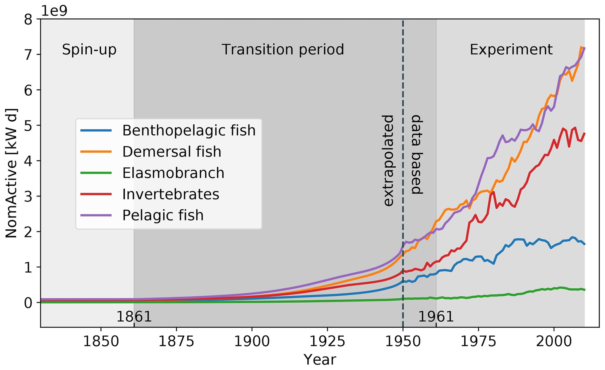
Figure 10Evolution of historical nominal active fishing effort (NomActive) as provided for the spin-up, transition period, and “obsclim + histoc; default” ISIMIP3a experiment, separated by target functional group. The groups represent an aggregation of 29 even finer categories covered by the dataset (see Table 17).

Download

Table 17Information about historical fishing intensities provided as DHF within ISIMIP3a. For the spin-up + transition period required by models within the marine ecosystems and fisheries sector the forcing is provided for 1841–2010, although the “obsclim + histoc; default” experiment only starts in 1961.

Download Print Version | Download XLSX

4.9 Fishing intensities

The dataset of reconstructed historical fishing efforts (Rousseau et al., 2022) serves as the DHF for the marine ecosystems and fisheries sector. The efforts are quantified separately for the artisanal and industrial fishing (sector), 66 large marine ecosystems (LMEs), 187 national exclusive economic zones (EEZs) and “high seas”, 244 country identifiers from the Sea Around Us Project (SAUP), 16 different categories of applied gear (e.g., bottom trawls, long lines, and purse seines), and 29 target functional groups (see nominal active fishing effort for five aggregated categories in Fig. 10).

The original annual time series spanning 1950–2015 were further extrapolated into the past to 1861 using generalized additive models (Rousseau et al., 2024; see Fig. 10). To cover the spin-up + transition period from 1841–1960 the dataset has been extended backwards by 1861 values. Forcing with this dataset allows for a comparison of simulated catches against the congruent (Watson, 2019) reconstruction of historical fishery catches (spanning the period 1869–2015; (Watson and Tidd, 2018). To permit integration into marine ecosystem models that capture different fishing sectors, fleets, and functional groups these data include nominal active fishing effort disaggregated by location (exclusive economic zone, high seas, and large marine ecosystem), fishing country, fishing gear, targeted functional group, and fishing sector (coastal artisanal and industrial). Impact modelers are allowed to distribute this effort across space and time, as well as to target organisms in any method compatible with their models' structure. The fishing effort data do not include any information about changes in the efficiency of fishing technology over time (technological creep). Assumptions about these efficiencies are left to the individual modelers and usually determined in model calibration.

Table 18Information about historical forest management provided as DHF for the regional forest sector within ISIMIP3a.

n/a: not applicable.

Download Print Version | Download XLSX

4.10 Forest management for the regional forest sector

For the regional forest sector, forest management is defined for nine forest sites in Europe, four of them in Germany (Peitz, KROOF, Solling beech, Solling spruce) and one each in the Czech Republic (Bily Kriz), Denmark (Sorø), France (Le Bray), Italy (Collelongo), and Finland (Hyytiälä) (Reyer et al., 2020b).

Additionally, a set of forest-site-specific management rules and planting numbers based on historical standard management practices of the area where the forest sites are located is defined and spelled out in concrete management schedules to enable modelers to simulate 2015soc conditions (Reyer et al., 2023). The regional forest management data have not been harmonized to the global gridded wood harvest data provided for the biomes sector because the data are very site-specific and the variation not resolved in the global dataset.