Earth System Model Aerosol–Cloud Diagnostics (ESMAC Diags) package, version 2: assessing aerosols, clouds, and aerosol–cloud interactions via field campaign and long-term observations

Tang, Shuaiqi; Varble, Adam C.; Fast, Jerome D.; Zhang, Kai; Wu, Peng; Dong, Xiquan; Mei, Fan; Pekour, Mikhail; Hardin, Joseph C.; Ma, Po-Lun

doi:https://doi.org/10.5194/gmd-16-6355-2023

Articles | Volume 16, issue 21

https://doi.org/10.5194/gmd-16-6355-2023

Articles | Volume 16, issue 21

Methods for assessment of models

08 Nov 2023

Methods for assessment of models |

| 08 Nov 2023

Earth System Model Aerosol–Cloud Diagnostics (ESMAC Diags) package, version 2: assessing aerosols, clouds, and aerosol–cloud interactions via field campaign and long-term observations

Shuaiqi Tang, Adam C. Varble, Jerome D. Fast, Kai Zhang, Peng Wu, Xiquan Dong, Fan Mei, Mikhail Pekour, Joseph C. Hardin, and Po-Lun Ma

Abstract

Poor representations of aerosols, clouds, and aerosol–cloud interactions (ACIs) in Earth system models (ESMs) have long been the largest uncertainties in predicting global climate change. Huge efforts have been made to improve the representation of these processes in ESMs, and the key to these efforts is the evaluation of ESM simulations with observations. Most well-established ESM diagnostics packages focus on the climatological features; however, they lack process-level understanding and representations of aerosols, clouds, and ACIs. In this study, we developed the Earth System Model Aerosol–Cloud Diagnostics (ESMAC Diags) package to facilitate the routine evaluation of aerosols, clouds, and ACIs simulated the Energy Exascale Earth System Model (E3SM) from the US Department of Energy (DOE). This paper documents its version 2 functionality (ESMAC Diags v2), which has substantial updates compared with version 1 (Tang et al., 2022a). The simulated aerosol and cloud properties have been extensively compared with in situ and remote-sensing measurements from aircraft, ship, surface, and satellite platforms in ESMAC Diags v2. It currently includes six field campaigns and two permanent sites covering four geographical regions: the eastern North Atlantic, the central US, the northeastern Pacific, and the Southern Ocean. These regions produce frequent liquid- or mixed-phase clouds, with extensive measurements available from the DOE Atmospheric Radiation Measurement user facility and other agencies. ESMAC Diags v2 generates various types of single-variable and multivariable diagnostics, including percentiles, histograms, joint histograms, and heatmaps, to evaluate the model representation of aerosols, clouds, and ACIs. Select examples highlighting the capabilities of ESMAC Diags are shown using E3SM version 2 (E3SMv2). In general, E3SMv2 can reasonably reproduce many observed aerosol and cloud properties, with biases in some variables such as aerosol particle and cloud droplet sizes and number concentrations. The coupling of aerosol and cloud number concentrations may be too strong in E3SMv2, possibly indicating a bias in processes that control aerosol activation. Furthermore, the liquid water path response to a perturbed cloud droplet number concentration behaves differently in E3SMv2 and observations, which warrants further study to improve the cloud microphysics parameterizations in E3SMv2.

Download & links

How to cite

How to cite.

Dates

Received: 08 Mar 2023 – Discussion started: 15 May 2023 – Revised: 29 Sep 2023 – Accepted: 02 Oct 2023 – Published: 08 Nov 2023

1 Introduction

Poor representations of aerosols, clouds, and aerosol–cloud interactions (ACIs) in Earth system models (ESMs) have long been the largest uncertainties in predicting global climate change (IPCC, 2021). Challenges come from several aspects, as outlined in the following. First, there are many aerosol properties (e.g., number, size, phase, shape, and composition) and cloud micro- and macro-physical properties (e.g., fraction, water content, and number and size of liquid and ice hydrometeors) that affect Earth's climate. Coincident measurements of these properties remain largely undersampled due to the substantial spatiotemporal variability and logistical difficulties involved with making such measurements. Second, there are complex interactive processes between aerosols, clouds, and ambient meteorological conditions, many of which are not fully understood but are critical to properly interpreting relationships between observable properties. Third, many ACI processes are nonlinear, multi-scale processes that involve feedbacks depending on cloud types and meteorological regimes, which also shift in space and time, presenting challenges with respect to assessing causal effect and representing such processes in ESMs.

Huge efforts have been made to improve the representation of aerosols, clouds, and ACIs in ESMs. The key to these efforts is the evaluation of ESM simulations with observations. Many modeling centers have developed standardized diagnostics packages to document ESM performance. For aerosol and cloud properties, most diagnostic packages rely heavily on satellite measurements as evaluation data (e.g., AMWG, 2021; E3SM, 2021; Eyring et al., 2016; Gleckler et al., 2016; Maloney et al., 2019; Myhre et al., 2013; Schulz et al., 2006). Satellite remote-sensing measurements have global or near-global coverage but limited spatial and temporal resolution. They are also facing many challenges to retrieve some variables, especially for aerosol properties such as number concentration, size distribution, and chemical composition. Some recent studies (e.g., Choudhury and Tesche, 2022) have retrieved the cloud condensation nuclei (CCN) number concentration from satellite measurements, which provides a great addition to investigate ACIs on the global scale. However, large uncertainties exist in satellite retrievals, even for more sophisticated retrieved cloud microphysical properties such as droplet number concentration (e.g., Grosvenor et al., 2018). This limits their application to robustly quantify aerosols, clouds, and ACI processes. In situ measurements from ground, aircraft, or ship platforms from field campaigns are also used in a few projects to evaluate ESMs (e.g., Reddington et al., 2017; Watson-Parris et al., 2019; Tang et al., 2022a; Zhang et al., 2020). Some of these field campaigns were conducted over remote or poorly sampled locations, which are highly valuable for model evaluation, despite limited spatial coverage and time periods. Moreover, the US Department of Energy (DOE) Atmospheric Radiation Measurement (ARM) user facility has conducted continuous field measurements at a few sites for multiple years. These long-term, high-resolution field measurements have also been demonstrated to be valuable for evaluating ESMs (e.g., Zhang et al., 2020).

In response to the need for more ESM diagnostics for evaluating ACI processes, Tang et al. (2022a) developed an ESM aerosol–cloud diagnostics (ESMAC Diags) package to facilitate the routine evaluation of aerosols, clouds, and ACIs simulated by the Energy Exascale Earth System Model (E3SM; Golaz et al., 2019) from the US DOE. It includes diagnostics that leverage in situ measurements from multiple platforms during six field campaigns since 2013, which have not been included in previous diagnostics tools (e.g., Reddington et al., 2017). Version 1 of ESMAC Diags (ESMAC Diags v1; Tang et al., 2022a) mainly focused on aerosol properties. Here, we present version 2 of ESMAC Diags (ESMAC Diags v2) that is a direct extension of ESMAC Diags v1 with two major additions:

measurements from satellite and long-term diagnostics at the ARM Southern Great Plains (SGP) and eastern North Atlantic (ENA) sites;
diagnostics for cloud properties and aerosol–cloud interactions.

The new measurements and major data quality controls are introduced in Sect. 2. Additional discussions on the retrieval uncertainties of cloud microphysical properties are performed in Sect. 3. Details of the code structure of ESMAC Diags v2, which has substantially changed since version 1, are described in Sect. 4. Section 5 provides selected examples of single-variable and multivariable diagnostics using ESMAC Diags v2 to highlight its capabilities. Lastly, Sect. 6 provides a summary.

2 Aerosol and cloud measurements from ground, aircraft, ship, and satellite platforms

Following the initial development in version 1, ESMAC Diags v2 continues to focus on six field campaigns conducted in four geographical regions: the central US (CUS, where the ARM Southern Great Plains, SGP, site is located), the eastern North Atlantic (ENA), the northeastern Pacific (NEP), and the Southern Ocean (SO). Information on the six field campaigns is shown in Table 1 and their locations are shown in Fig. 1, reproduced from Table 1 and Fig. 3 in Tang et al. (2022a), respectively.

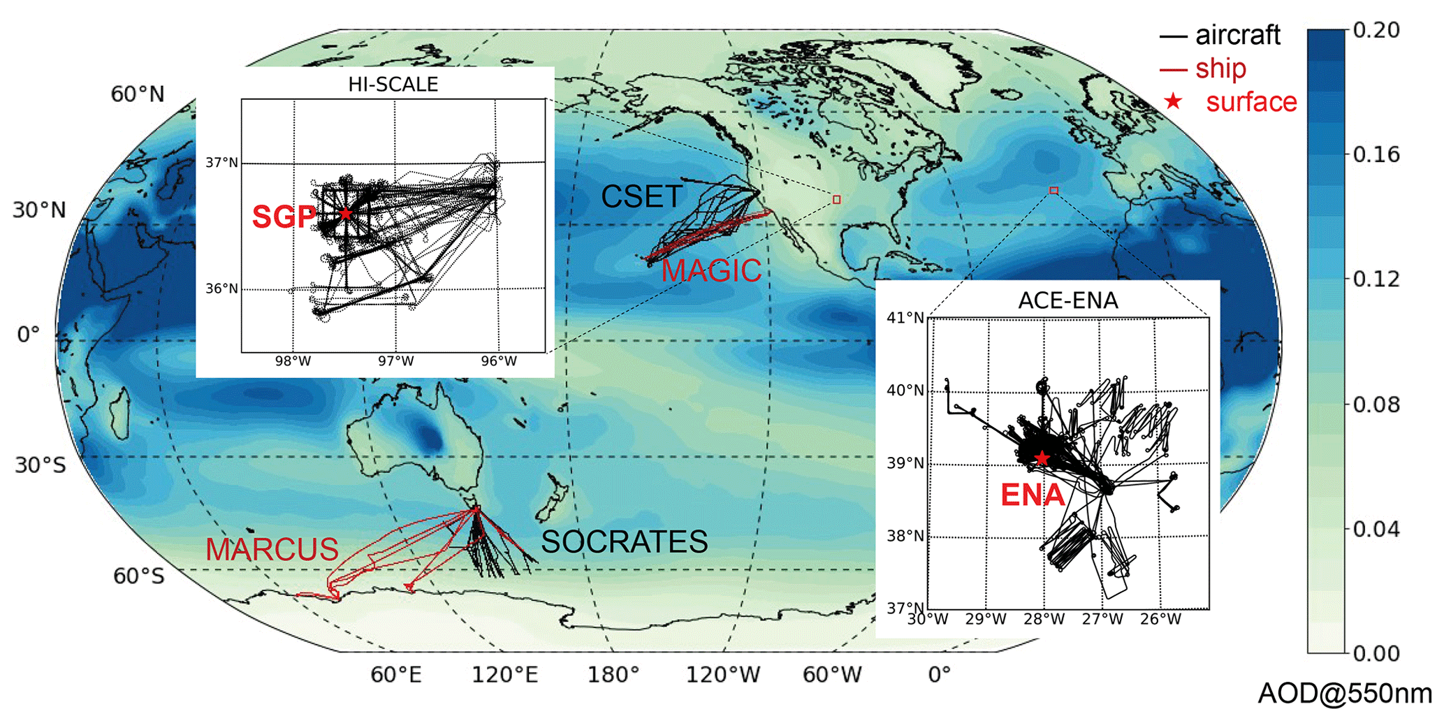
https://gmd.copernicus.org/articles/16/6355/2023/gmd-16-6355-2023-f01

Figure 1Aircraft (black) and ship (red) tracks for the six field campaigns. Red stars on the enlarged map indicate two ARM fixed sites that have long-term measurements available for model diagnostics: SGP and ENA. Overlaid is aerosol optical depth at 550 nm averaged from 2014 to 2018 simulated in E3SMv1. (The figure is reproduced from Fig. 3 in Tang et al., 2022a.)

Table 1Descriptions of the field campaigns used in this study. (The table is reproduced from Table 1 in Tang et al., 2022a.)

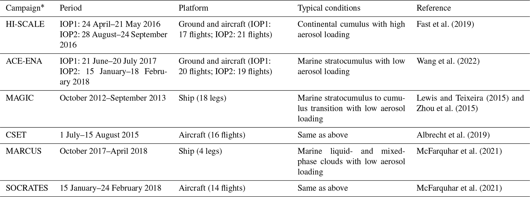
^* Full names of the listed field campaigns: HI-SCALE – Holistic Interactions of Shallow Clouds, Aerosols, and Land Ecosystems; ACE-ENA – Aerosol and Cloud Experiments in the Eastern North Atlantic; MAGIC – Marine ARM GPCI Investigation of Clouds; CSET – Cloud System Evolution in the Trades; MARCUS – Measurements of Aerosols, Radiation, and Clouds over the Southern Ocean; SOCRATES – Southern Ocean Cloud Radiation and Aerosol Transport Experimental Study.

Download Print Version | Download XLSX

The collection and processing of observations are the most time-consuming part of developing ESMAC Diags, and these processes also impact the reliability of conclusions drawn from the model diagnostics. In this section, we introduce the data used in ESMAC Diags v2, existing quality issues in some datasets, and treatments to address these quality issues. Some variables are difficult to directly measure or have limited in situ sampling and, thus, must be derived from remote-sensing measurements using retrieval algorithms. In Sect. 3, we further discuss the uncertainty and reliability of some cloud retrieval products via comparisons with in situ aircraft measurements.

2.1 Data availability

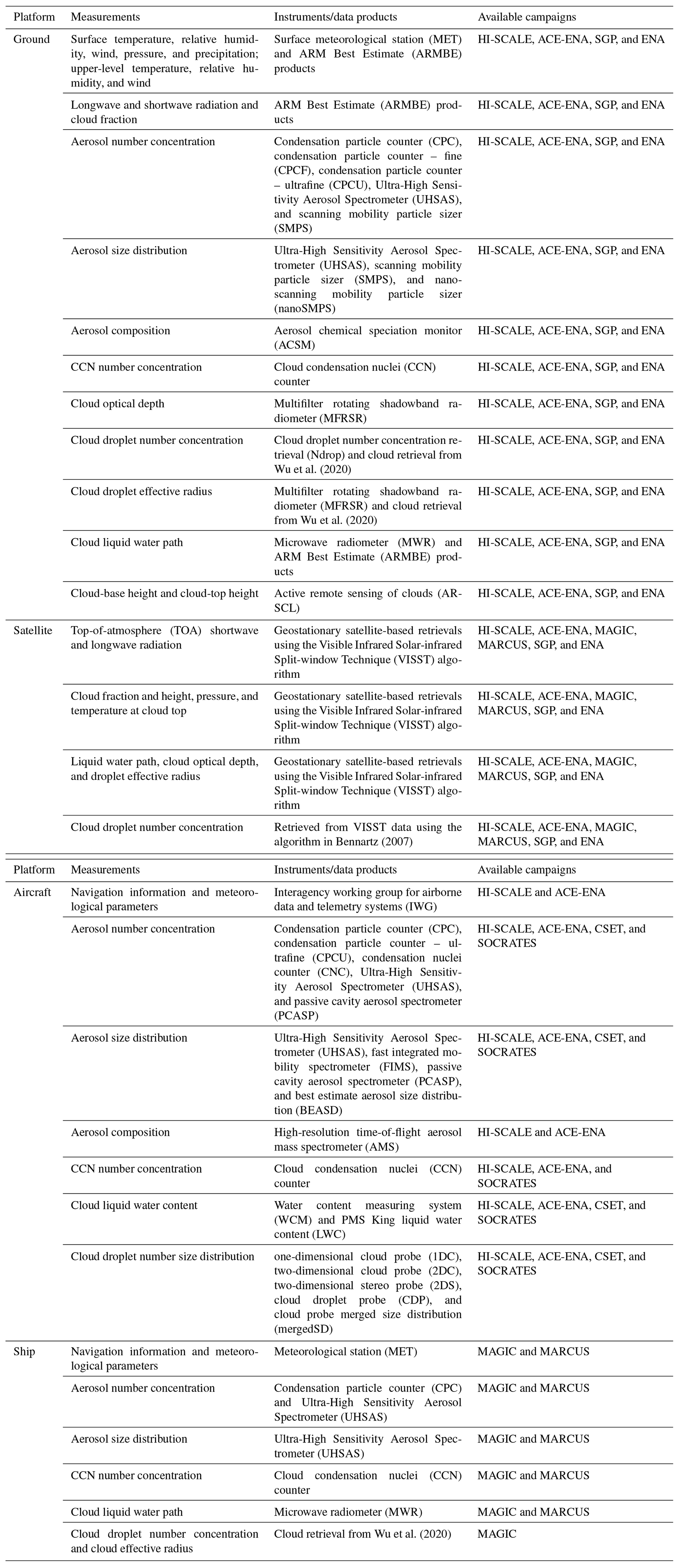
All measurements, instruments, and data products used in the six field campaigns and two long-term sites in ESMAC Diags v2 are shown in Table 2. Further details of the measurements, data product names, and DOIs are given in Tables S1 to S6 (for field campaigns) and Tables S7 and S8 (for SGP and ENA sites) in the Supplement. To allow for the maximum overlap of key measurements while also ensuring a long enough period for statistical evaluation, we select the periods of 1 January 2011–31 December 2020 for SGP and 1 January 2016–31 December 2018 for ENA for long-term analyses. In addition to the aerosol measurements discussed in Tang et al. (2022a), we incorporate more cloud and radiation measurements as well as geostationary satellite retrievals using the Visible Infrared Solar-infrared Split-window Technique (VISST) (Minnis et al., 2008, 2011) algorithm. The VISST products archived by ARM cover approximately 10^∘ × 10^∘ regions at a 0.5^∘ × 0.5^∘ resolution centered over ARM sites. Moreover, ARM recently released products consisting of merged aerosol particle and cloud droplet size distributions from aircraft measurements for the HI-SCALE and ACE-ENA campaigns. These data are now used in ESMAC Diags v2.

Table 2List of instruments and measurements used in ESMAC Diags v2.

Download XLSX

All of the observational data are quality controlled with their time resolution rescaled to that suitable for evaluating E3SM, and the rescale resolution can be adjusted to fit different model output frequencies. Currently, ground, ship, and satellite measurements are rescaled to a 1 h frequency to be consistent with the current E3SM output frequency. Rescaling consists of computing either the median, mean, or interpolated value depending on the original data frequency and variable properties. For most aerosol and cloud microphysics measurements, the median value is computed to remove occasional spikes or zeros resulting from data contamination or measurement error. For some bulk cloud properties (e.g., cloud fraction or liquid water path – LWP), the mean value is computed to be consistent with the grid-mean E3SM output. Interpolation is only used when the input frequency is equal to or coarser than the frequency of model output. For aircraft measurements, a 1 min resolution is used to retain high variability and allow the matching of samples of aerosol and cloud at the same time. For comparison with high-frequency aircraft data, E3SM output is interpolated to the same resolution using the nearest grid cell and time slice. Although the current 1 h, 1^∘ E3SM output could not capture the high variability in the aircraft measurements, we are targeting the exascale E3SM version planned in the next few years. In kilometer-scale-resolution ESM simulations, the high variability in aircraft measurements will be better captured. In the current diagnostics, we only focus on the statistics for the entire campaign. As seen later in Sect. 5.1, coarse-resolution model output shows similar percentile ranges with the high-resolution aircraft measurements, indicating that, for simple percentiles, large-scale variabilities dominate over sub-grid variabilities over monthlong field campaign periods. Further analysis is needed to understand the importance of other statistics (e.g., variance and covariance) of sub-grid-scale variabilities. All of the processed data are saved in a standardized network common data form (NetCDF) format (NETCDF, 2022) and are available for download (see the “Data availability” section) and direct use.

2.2 Data quality issues and treatments

Many observation datasets used in ESMAC Diags are ARM level-b (quality-controlled) or level-c (value-added) products, which include quality control (QC) flags to indicate data quality issues. For most datasets, a QC treatment is applied to remove all data with questionable flags. However, there are certain datasets or circumstances in which a QC flag is overly strict (too many good data are removed) or not strict enough (some bad data are not removed). Here, we document some of these situations and how we handle them in our data processing.

2.2.1 ARM condensation particle counter (CPC) measurements

ARM CPC data have several QC values representing the failure of different quality checks. One of the checks establishes if the concentration is greater than a maximum allowable value, which is set to 8000 cm⁻³ for model 3010 (CPC, size detection limit 10 nm), 10 000 cm⁻³ for model 3772 (CPCF, size detection limit 10 nm), and 50 000 cm⁻³ for model 3776 (CPCU, size detection limit 3 nm). At SGP, new particle formation (NPF) events occur frequently during which CPC and CPCF measurements can exceed 30 000 cm⁻³. This is much higher than the maximum allowable value but physically reasonable. Simply removing these large values results in an underestimation of the aerosol number concentration and produces an unrealistic diurnal cycle, as they usually occur during the daytime (Tang et al., 2022a). After consultation with the ARM instrument mentor, we only remove data with critical QC flags but keep data with this QC flag that is overly restrictive.

2.2.2 National Center for Atmospheric Research (NCAR) research flight aerosol number concentration (CN) measurements

NCAR research flight (RF) data used in ESMAC Diags do not include QC flags but occasionally show suspiciously large or negative aerosol counts. The following minimum and maximum thresholds are applied to remove suspicious data:

total CN from a condensation nucleation counter (CNC, reported as CONCN), minimum of 0 and maximum of 25 000 cm⁻³;
total CN from an Ultra-High Sensitivity Aerosol Spectrometer (UHSAS, reported as UHSAS100), minimum of 0 and maximum of 5000 cm⁻³;
aerosol number size distribution from an UHSAS (reported as CUHSAS_RWOOU or CUHSAS_LWII), minimum of 0 and maximum of 500 cm⁻³ per size bin.

2.2.3 Ship-measured aerosol properties

Aerosol instruments on ships are occasionally contaminated by ship emissions, which present as large spikes in aerosol and CCN number concentrations. For ARM MARCUS measurements, Humphries (2020) published reprocessed CN and CCN data to remove ship exhaust contamination using method described in Humphries et al. (2019). These data are used in this diagnostics package. For MAGIC, we could not find any ship exhaust contamination information. By visually examining the dataset, a simple maximum threshold (25 000 cm⁻³ for CPC, 5000 cm⁻³ for UHSAS100, 2000 cm⁻³ for CCN at 0.1 % supersaturation, and 4000 cm⁻³ for CCN at 0.5 % supersaturation) is applied to remove likely contamination from ship emissions.

2.2.4 CCN measurements

There are different supersaturation (SS) setting strategies for CCN measurements. Some aircraft campaigns measured CCN with constant SS (ACE-ENA and HI-SCALE). Some other campaigns measured CCN with time-varying (scanning) SS (SOCRATES, surface CCN counters at SGP and ENA). However, the actual SS in a scanning strategy has fluctuations that are different from the target SS. For the latter, CCN for each SS (0.1 %, 0.2 %, 0.3 %, and 0.5 %) are obtained by selecting CCN measured within ±0.05 % of the SS target.

For long-term measurements at SGP and ENA, near-hourly CCN spectra data are available, and a quadratic polynomial is fit to the spectra such that the CCN number concentration can be estimated at any SS between the measured minimum and maximum SS values. We calculate and output CCN number concentration from these fits at three target supersaturations (0.1 %, 0.2 %, and 0.5 %). The fitted spectra data provide the CCN number concentration at the exact target supersaturations, but the sample number is slightly smaller due to the occasional failure of polynomial fitting.

2.2.5 Contaminated surface aerosol measurements at ENA

The ARM ENA site is located at a local airport. Aerosol measurements at ENA are sometimes contaminated by aircraft and vehicle emissions, rendering the measurements unrepresentative of the background environment. Gallo et al. (2020) identified periods when CPC measurements were likely contaminated from localized emissions (Fig. 2a). Their aerosol mask data have a 1 min resolution. When we rescale the data to a 1 h resolution and apply the mask on other coarse-time-resolution aerosol measurements (e.g., ACSM; Fig. 2c), we mask hours in which more than half of the hour is flagged by the aerosol mask. The masking slightly increases the occurrence fraction of small values due to removing many large values, but it does not change the overall distribution (Fig. 2b, d). A sensitivity analysis was performed, showing that 50 % is a reasonable threshold to balance the removal of contamination with the conservation of reasonable data (not shown).

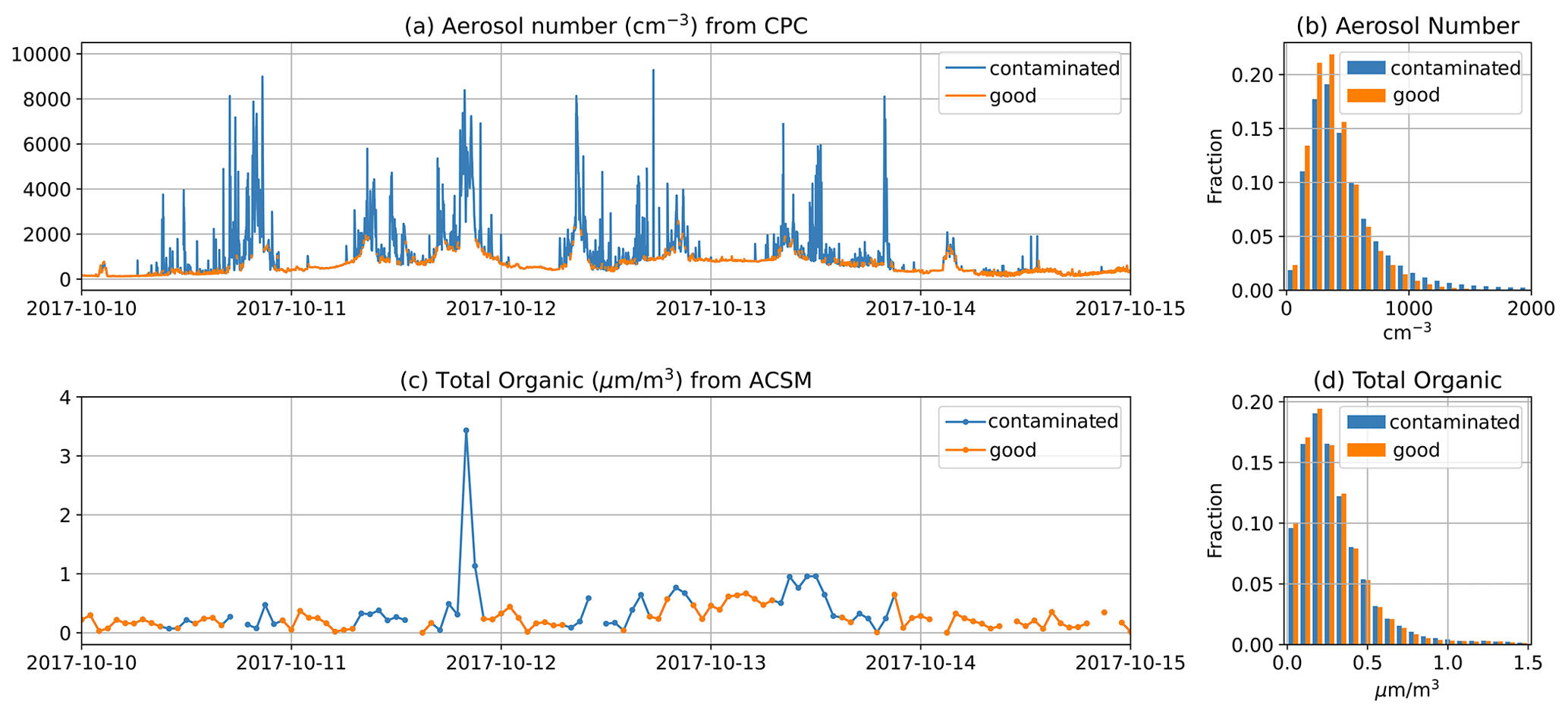
https://gmd.copernicus.org/articles/16/6355/2023/gmd-16-6355-2023-f02

Figure 2(a) CPC-measured CN from 10 to 15 October 2017 (1 min resolution) with local contamination flagged by Gallo et al. (2020). (b) Histogram of CPC-measured CN for all data from 2016 to 2018. (c) ACSM-measured total organic matter from 10 to 15 October 2017 (1 h resolution). Hours with more than half of the hour flagged in 1 min CPC data are masked as contaminated. (d) Histogram of ACSM-measured total organic matter for all data from 2016 to 2018.

Download

3 Verification of cloud retrievals with in situ measurements

Cloud microphysical properties such as the droplet number concentration (N_d) and effective radius (R_eff) are important variables that connect clouds to other aspects in the climate system such as aerosols and radiation. Except in field campaigns where in situ aircraft measurements are available, remote-sensing retrieval algorithms are usually needed to derive these quantities. Several cloud retrieval products from ground and satellite measurements with different algorithms are used in ESMAC Diags v2. This section compares these cloud retrievals with in situ aircraft measurements to assess retrieval limitation, uncertainty, and utility. N_d and R_eff from aircraft measurements taken during the HI-SCALE and ACE-ENA field campaigns are calculated from merged cloud droplet number size distributions (mergedSD) from three different cloud probes with different size ranges. The mergedSD product comprises the size range from 1.5 to 9075 µm, covering the entire E3SM cloud droplet size distribution range and extending to the rain droplet size range (> 100 µm). For field campaigns used in this study, the aircraft only flew through non-precipitating or drizzling clouds, in which the airborne measurements usually measure rain droplet numbers 3 to 5 orders of magnitude smaller than the cloud droplet number. Therefore, the inclusion of the rain droplet size range has an ignorable impact on the aircraft-estimated N_d and R_eff.

Table 3 lists the R_eff and N_d retrieval products used in ESMAC Diags v2. We retrieved Nd_sat with input data from VISST products using the algorithms described in Bennartz (2007) but assuming a drop volume mean radius to R_eff ratio (commonly referred to as k) of 0.74 and a cloud adiabaticity of 80 % (Varble et al., 2023). Other datasets are all available as released products. All retrievals assume a horizontally homogeneous single-layer liquid-phase cloud with constant N_d throughout the cloud layer. However, retrieval algorithms are usually run for all conditions whenever they return valid values. When assumptions are not satisfied, retrieved properties may contain large errors and likely alter statistics, such as increasing the occurrence frequency of small N_d, as will be shown next.

Table 3Cloud droplet effective radius (R_eff) and number concentration (N_d) retrievals.

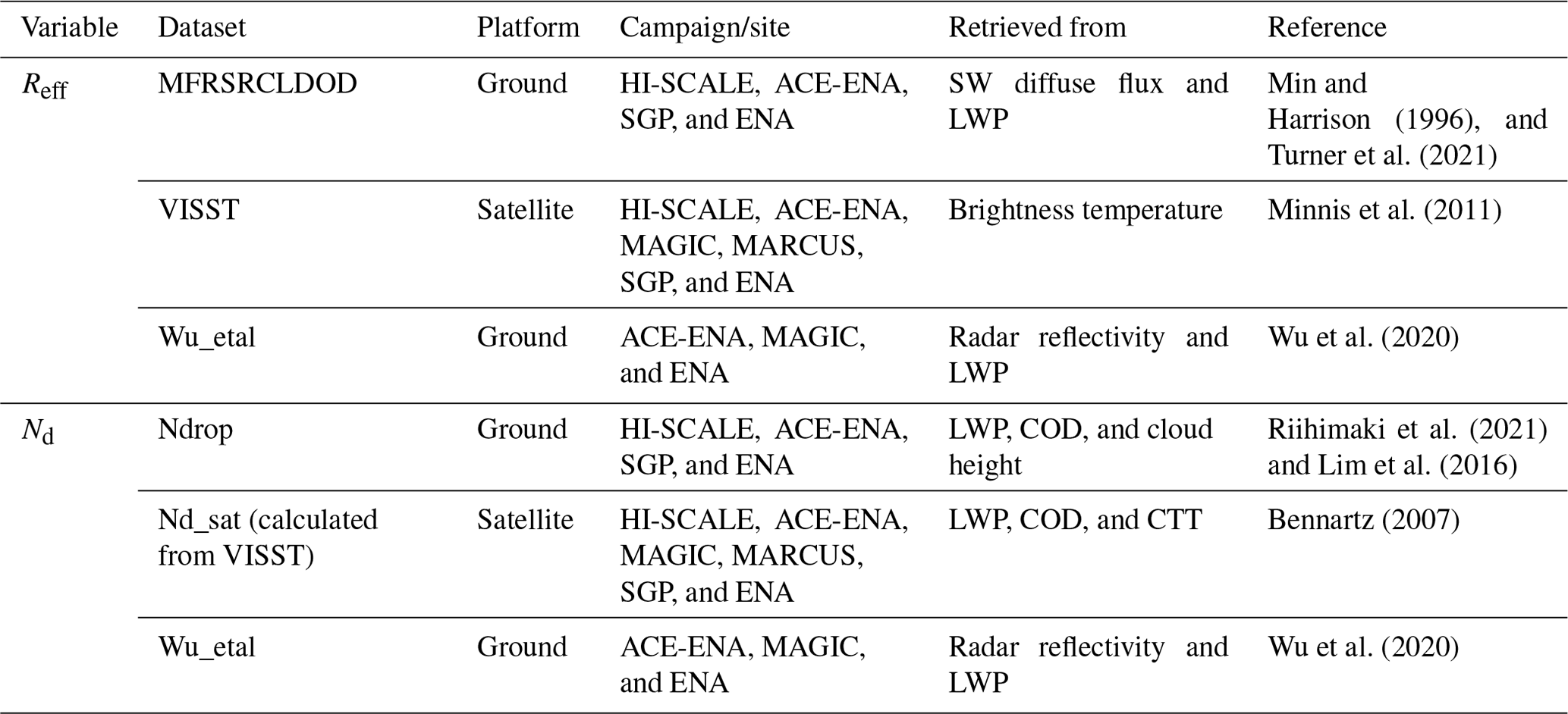
The abbreviations/acronyms used in the table are as follows: MFRSRCLDOD – Cloud Optical Properties from the Multifilter Rotating Shadowband Radiometer (MFRSR); SW – shortwave; COD– cloud optical depth; CTT – cloud-top temperature.

Download Print Version | Download XLSX

Figure 3 shows the occurrence fraction histograms of N_d retrievals with aircraft measurements for the HI-SCALE and ACE-ENA field campaigns, with the comparison of the original temporal resolution versus the 30 min mean, and the use of all available samples and samples that are filtered as overcast (cloud fraction > 90 %) low-level cloud (cloud-top height < 4 km) conditions. Figure 4 shows similar plots but for R_eff. We also selected two cases with single-layer boundary layer stratus or stratocumulus clouds and plotted their time series of original-resolution and 30 min averaged R_eff and N_d in Fig. S1 in the Supplement. The high-frequency aircraft measurements and MFRSR/Ndrop retrievals exhibit much larger variability than the coarse-frequency retrievals of Wu_etal and VISST. They frequently sample cloud edges or cloud top/cloud base (for aircraft), where N_d values are typically lower than those further into the cloud. This causes large occurrence fractions in the lowest few bins in the N_d histograms (Fig. 3a, d). The 30 min VISST products also show a large occurrence fraction in the lowest N_d bin for HI-SCALE (Fig. 3a), likely due to the high frequency of partially cloudy conditions over the continental US. Filtering conditions to only include overcast, low-level cloud conditions (Fig. 3b, e) and averaging into a coarser resolution (Fig. 3c, f) both contribute to the reduction in the occurrence fraction in small-N_d bins and make the measurements from different instruments more comparable.

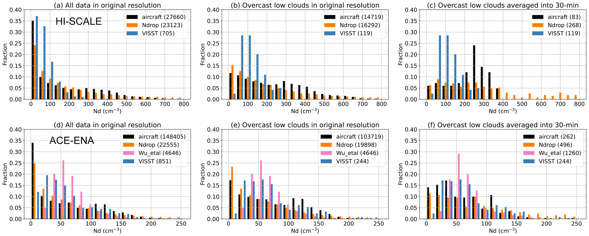
https://gmd.copernicus.org/articles/16/6355/2023/gmd-16-6355-2023-f03

Figure 3Histogram of N_d from different measurements/retrievals from the (a, b, c) HI-SCALE and (d, e, f) ACE-ENA field campaigns, with total sample numbers given in parentheses. Panels (a) and (d) use data samples in their original resolution (1 s for aircraft measurements, 20 s for Ndrop data, 5 min for Wu_etal data, and 30 min for VISST data). Panels (b) and (e) include only overcast, low-cloud situations. For aircraft data, this means that N_d is > 1 cm⁻³ for 5 s before and after the sampling time; for Ndrop and VISST data, it means that the cloud fraction > 90 % and the cloud-top height < 4 km. Panel (c) and (f) include only overcast, low-cloud situations, and they average them into a 30 min resolution. For all of the plots, VISST data with a solar zenith angle > 65^∘ are removed to avoid artifacts due to sunlight.

Download

https://gmd.copernicus.org/articles/16/6355/2023/gmd-16-6355-2023-f04

Figure 4Similar to Fig. 3 but for R_eff.

Download

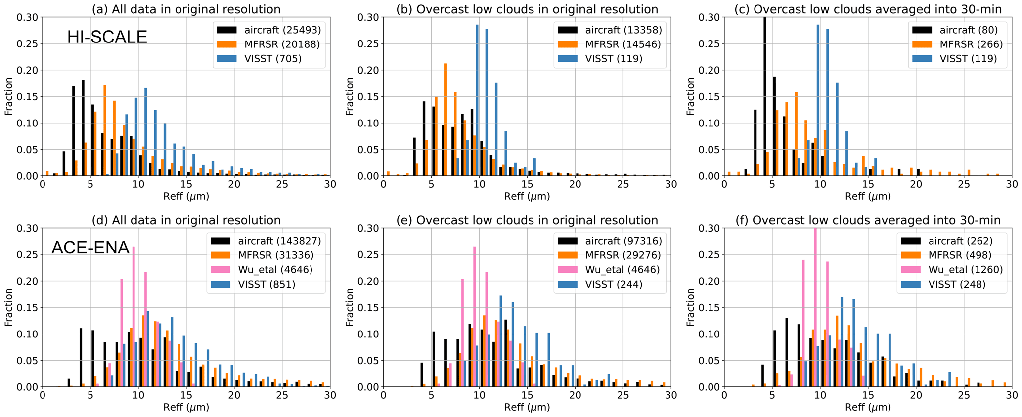
Overall, the remote-sensing retrievals and aircraft measurements produce reasonable ranges of N_d and R_eff. Marine clouds (ACE-ENA) have smaller N_d (Fig. 3) and larger R_eff (Fig. 4) values than continental clouds (HI-SCALE). Different retrievals are more consistent with each other for marine clouds than for continental clouds. Even after rescaling to the same temporal resolution, aircraft and Ndrop data exhibit broader N_d distributions than satellite retrieval data, likely due to their high sampling frequency that may capture more extreme conditions with very high or low N_d values. Moreover, the assumption of a fixed adiabaticity (0.8) in satellite retrieval data will also narrow the N_d distribution. For R_eff, we do not expect different datasets to agree perfectly with each other, as the cloud droplet size grows with height in the cloud. All remote-sensing retrievals have larger R_eff values than aircraft measurements, potentially because remote sensors are more sensitive to the upper cloud where the droplet size and liquid water content (LWC) are larger. Wu_etal retrieves vertical profiles of R_eff, and a median value of the R_eff profile is used to represent the entire cloud. This makes the Wu_etal retrieval less sensitive to large droplets; thus, its R_eff is less than MFRSR and VISST. VISST data have the largest R_eff values, likely because satellite retrievals reflect conditions at the cloud top. Given the spread in retrieved cloud properties, the limitations and uncertainties of cloud microphysics retrievals clearly need to be considered when they are used to evaluate model performance.

4 Structure of the diagnostics package

Figure 5 shows the directory structure of ESMAC Diags v2. It is substantially changed compared with ESMAC Diags v1 (Tang et al., 2022a). First, we save all data separately as raw_data, which stores all input datasets collected from field campaigns, and prep_data, which stores preprocessed data with a standardized time resolution and quality controls, as described in Sect. 2. The structure is still designed to be flexible for future extension with additional measurements and/or functionality. Second, the diagnostics functions now give users more freedom to modify analyses, such as selecting different time periods, performing additional data filtering or treatments, and examining ACI relationships in specified variable combinations (for scatterplots, joint histograms, or heatmaps). We provide a set of example scripts to assist users with designing their own diagnostics based on their needs. We also provide the source code of data preparation for observations and model output as well as detailed instructions on how to run the code. Users can revise the code to process their own observational data or model output. All of the information is available in the ESMAC Diags GitHub repository.

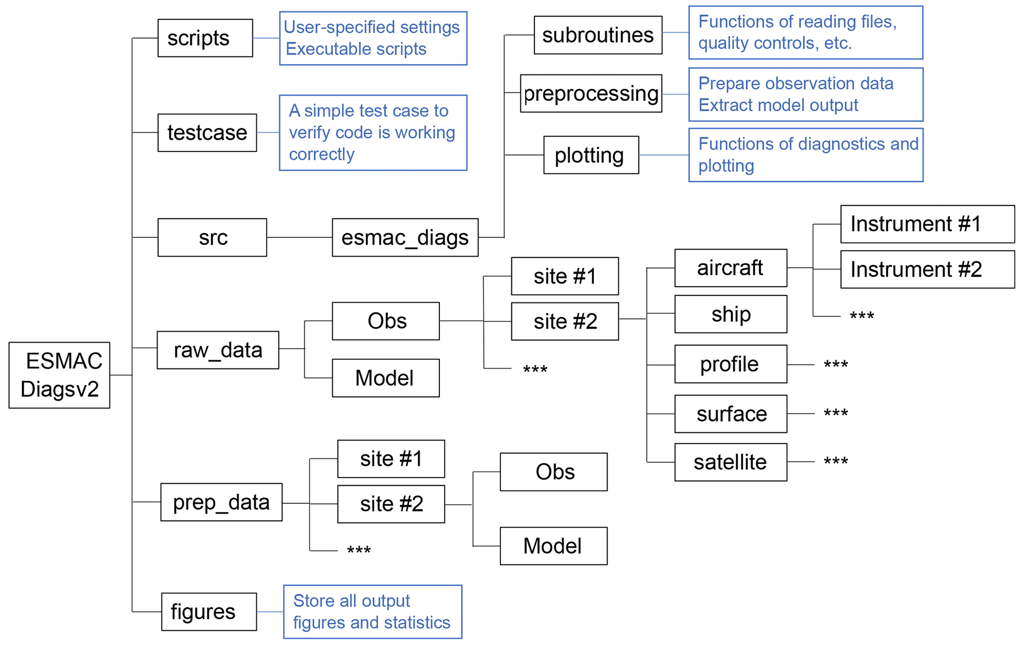
https://gmd.copernicus.org/articles/16/6355/2023/gmd-16-6355-2023-f05

Figure 5Directory structure of ESMAC Diags v2. Blue boxes describe the functions of the directory. Asterisks represent boxes that follow the same format as those shown in parallel.

Download

ESMAC Diags v1 included diagnostics of aerosol mean statistics (mean, bias, RMSE, and correlation), time series, diurnal cycle, vertical profiles, mean particle number size distribution, percentiles by height/latitude, and pie/bar charts (Tang et al., 2022a). ESMAC Diags v2 now comprises the following new diagnostics that include cloud variables:

5th, 25th, 50th, 75th, and 95th percentiles;
seasonal cycle at SGP and ENA;
histograms for individual variables;
scatterplots;
joint histograms of two variables; and
heatmaps of three variables (mean of one variable binned by two other variables).

The inclusion of two-variable scatterplots, joint histograms, and three-variable heatmaps provides the functionality to study ACI-related relationships. We present a few examples in the next section to demonstrate these new diagnostics.

5 Diagnostics examples

In this section, we show some examples of diagnostics applied to E3SM version 2 (E3SMv2; Golaz et al., 2022). Compared with the aerosol and cloud parameterizations in E3SMv1 (Rasch et al., 2019; Golaz et al., 2019), E3SMv2 updated the treatments of dust particles, incorporated recalibration of parameters (Ma et al., 2022), changed the call order and refactored the code of the Cloud Layers Unified By Binormals (CLUBB) parameterization, and retuned some parameters (Golaz et al., 2022). We constrain the model simulations by nudging the horizontal winds towards the 3-hourly Modern-Era Retrospective analysis for Research and Applications, Version 2 (MERRA-2; Gelaro et al., 2017) with a nudging timescale of 6 h. Previous studies have shown that, with nudging, E3SM can simulate the large-scale circulations in reanalyses well (Sun et al., 2019; Zhang et al., 2022). The model was run for individual field campaigns (Table 1) and from 2010 to 2020 for long-term diagnostics at the SGP and ENA sites, with hourly model output saved over the field campaign regions for detail evaluation. As described in Sect. 2, all diagnostics for ground and ship campaigns are at a 1 h resolution, whereas diagnostics for aircraft campaigns are at a 1 min resolution. For aerosol and cloud variables, model raw output variables (not from instrument simulators) are used in this paper to reveal the intrinsic ACI relationships in E3SM. However, as can be seen later in this section, instrument simulators can be better used in some diagnostics to ensure more consistent comparison. Users may choose whether or not to use simulators in their diagnostics depending on their purpose.

5.1 Single-variable diagnostics

Figures 6 and 7 show mean and percentile values of aerosol and cloud properties measured from field campaigns in the four geographical regions: CUS, ENA, NEP, and SO. Figure 6 is for aircraft platforms, whereas Fig. 7 is for ground or ship platforms; satellite data are also included in Fig. 7 when available. Note that the aircraft and ground/ship campaigns may cover different time periods (Table 1); thus, some differences seen between aircraft and ship measurements may be caused by seasonal variation. As cloud microphysical properties are usually retrieved with assumptions (Sect. 3), for ground/ship/satellite data, we only focus on overcast, low-level, liquid-cloud conditions here (cloud fraction > 90 %, cloud-top height < 4 km, and ice water path < 0.01 mm). E3SM does not output cloud-top height, which is derived using a weighted integration method, as described in Varble et al. (2023). From both aircraft and ground/ship data, HI-SCALE has much larger aerosol and cloud droplet number concentrations as well as smaller droplet sizes compared with other campaigns, which is expected for a continental environment compared with a marine environment. The cloud optical depth is also greater for HI-SCALE than for other campaigns, which is driven by smaller droplet sizes rather than LWP differences. Satellite retrievals generally produce smaller N_d, LWP, and cloud optical depth values with greater R_eff values than surface retrievals. As discussed in Sect. 3, retrieval uncertainties need to be kept in mind when these retrieved microphysical properties are used to evaluate models.

E3SMv2 overestimates CN (> 10 nm) over CUS, ENA, and NEP. Larger-particle (CN > 100 nm) concentration is generally underestimated over CUS and overestimated over ENA and NEP. Over SO, E3SMv2 produces fewer small aerosol particles (CN > 10 nm) and about the same number of large aerosol particles (CN > 100 nm) compared to the observations. These results are confirmed by both aircraft and ground/ship campaigns, except for the HI-SCALE aircraft campaign in which small particles from local emissions were occasionally observed but were unable to be simulated. These results are consistent with our previous diagnostics for E3SMv1 (Tang et al., 2022a). E3SMv2 also underestimates N_d over CUS and SO, which corresponds to the underestimation of accumulation-mode (> 100 nm) CN over CUS but the underestimation of Aitken-mode (> 10 nm) CN over SO. It is possible that small particles are more important in cloud formation over very clean regions such as SO than over continental regions such as CUS. The simulated LWP (LWC) is generally consistent with satellite (aircraft) measurements but smaller than ground/ship measurements, which may be partly caused by rain contamination of ground/ship retrievals. R_eff evaluation is less certain given large discrepancies between satellite and ground retrievals.

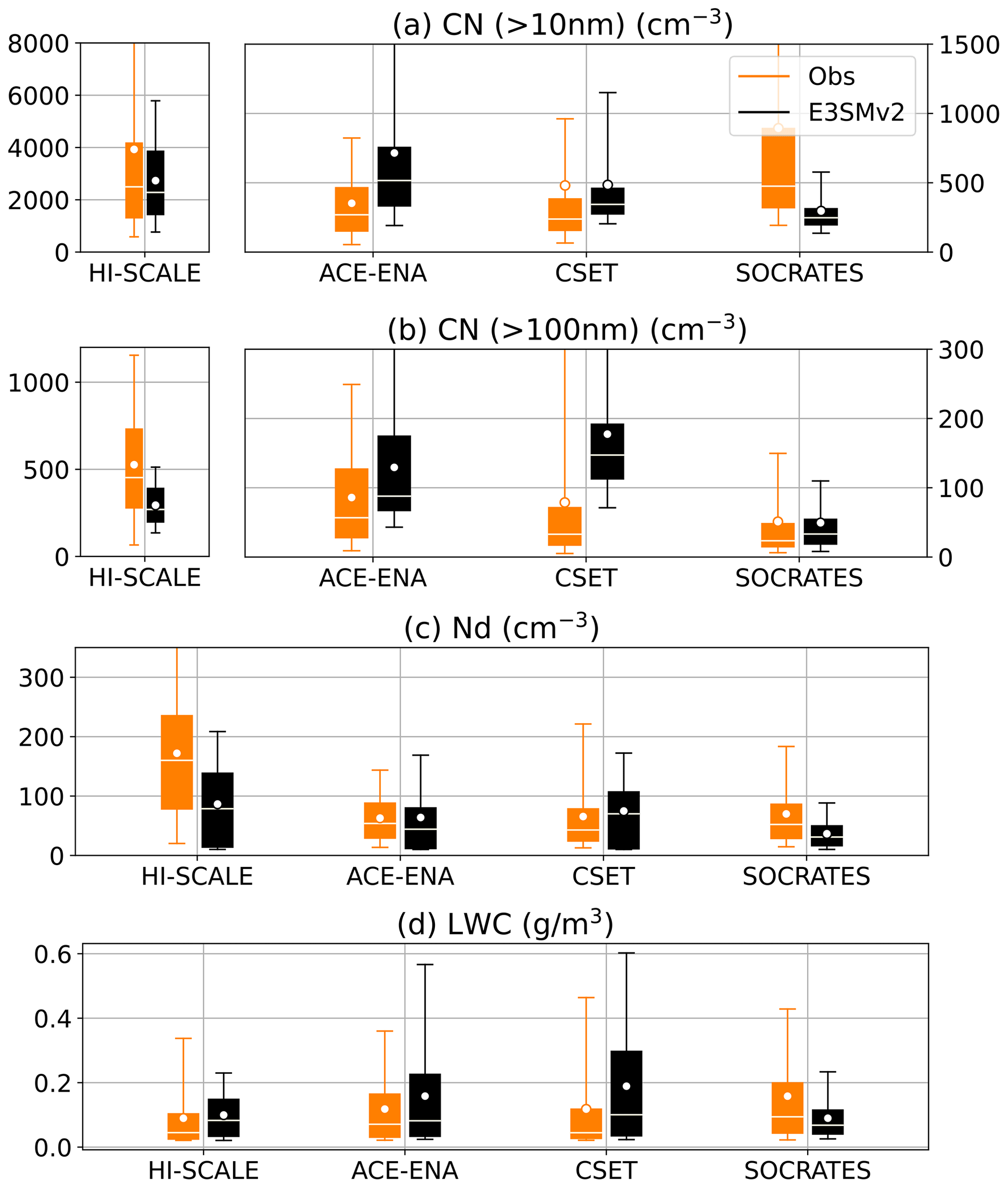
https://gmd.copernicus.org/articles/16/6355/2023/gmd-16-6355-2023-f06

Figure 6Box-and-whisker plots of (a) CN for size > 10 nm, (b) CN for size > 100 nm, (c) in-cloud N_d, and (d) LWC for all data from aircraft field campaigns in the CUS, ENA, NEP, and SO regions (from left to right). Boxes denote the 25th and 75th percentiles, whiskers denote the 5th and 95th percentiles, the white horizontal lines represent median values, and the white dots represent mean values. For aerosol number concentrations, the y axes for HI-SCALE are separated from other field campaigns for better visualization. The top whiskers that are out of the y-axis range are HI-SCALE – Obs (13681), ACE-ENA – E3SMv2 (2061), and SOCRATES – Obs (2745) in panel (a); ACE-ENA – E3SMv2 (304), CSET – Obs (305), and CSET – E3SMv2 (400) in panel (b); and HI-SCALE – Obs (397) in panel (c).

Download

https://gmd.copernicus.org/articles/16/6355/2023/gmd-16-6355-2023-f07

Figure 7Box-and-whisker plots of (a) CN for size > 10 nm, (b) CN for size > 100 nm, (c) layer-mean N_d, (d) LWP, (e) R_eff, and (f) cloud optical depth for overcast, low-level, liquid-cloud conditions (cloud-top height < 4 km, cloud fraction > 90 %, and ice water path < 0.01 mm) for ground- and ship-based field campaigns in the CUS, ENA, NEP, and SO regions (from left to right). Boxes denote the 25th and 75th percentiles, whiskers denote the 5th and 95th percentiles, the white horizontal lines represent median values, and the white dots represent mean values. For aerosol number concentrations, the y axes for HI-SCALE are separated from other field campaigns for better visualization. The top whiskers that are out of the y-axis range are HI-SCALE – E3SMv2 (6102), ACE-ENA – E3SMv2 (7575), MAGIC – Obs (3330), and MAGIC – E3SMv2 (3771) in panel (a); ACE-ENA – Obs (304.7), ACE-ENA – E3SMv2 (328.3), MAGIC – Obs (377.7), and MAGIC – E3SMv2 (577.8) in panel (b); and HI-SCALE Obs (670.9) in panel (c).

Download

https://gmd.copernicus.org/articles/16/6355/2023/gmd-16-6355-2023-f08

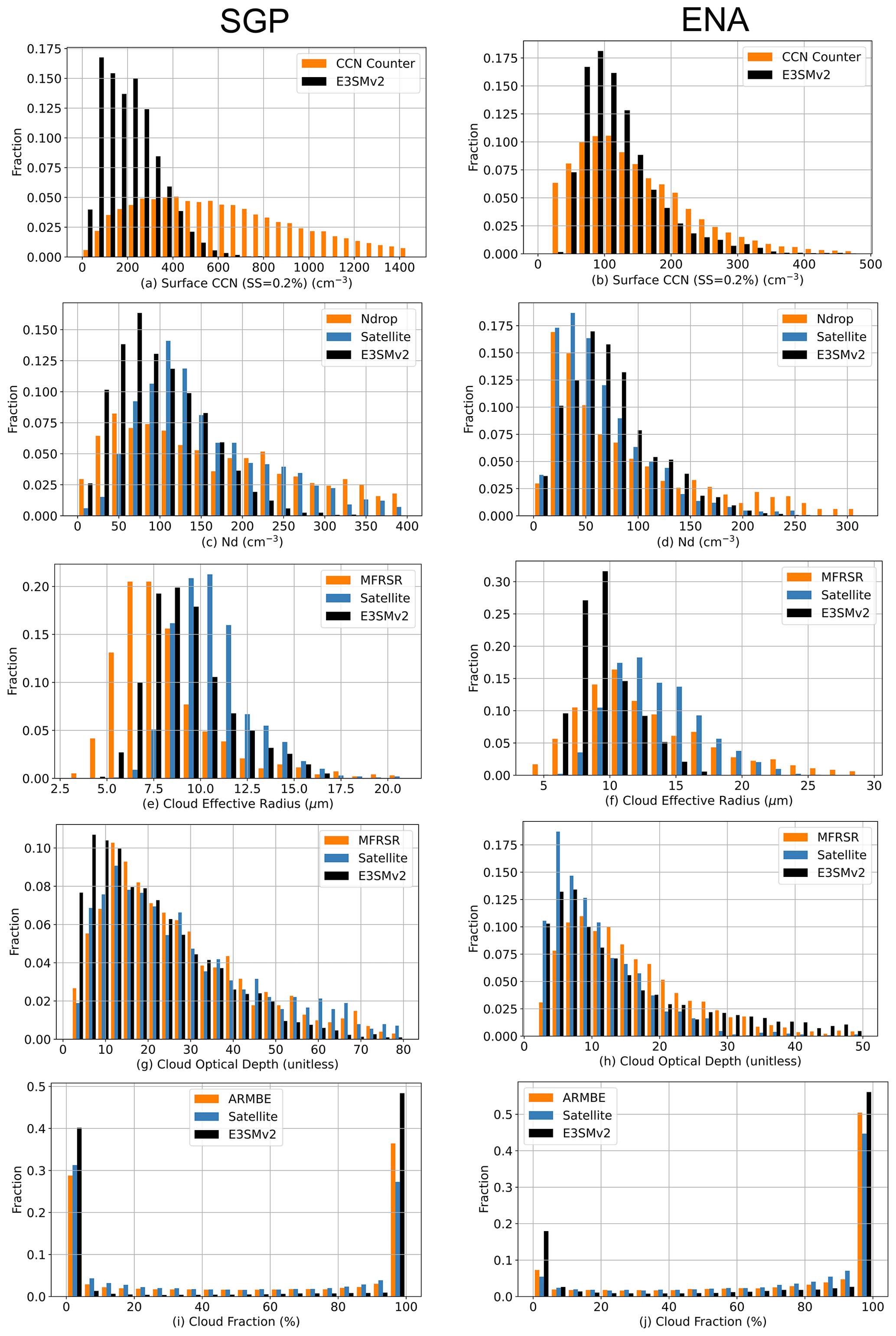
Figure 8Histogram of (from top to bottom) surface CCN number concentration, layer-mean N_d, R_eff, cloud optical depth, and total cloud fraction at (left) SGP from 2011 to 2020 and (right) ENA from 2016 to 2018. The surface CCN and total cloud fraction are using all-condition samples, whereas N_d, R_eff, and cloud optical depth data are filtered for overcast, low-level, liquid-cloud conditions (cloud-top height < 4 km, cloud fraction > 90 %, and ice water path < 0.01 mm).

Download

Figure 8 shows histograms of the surface CCN number concentration at 0.2 % supersaturation, cloud-layer-mean N_d, R_eff, cloud optical depth, and total cloud fraction for long-term diagnostics at the SGP (2011–2020) and ENA (2016–2018) sites. E3SMv2 fails to reproduce the long tail of large CCN and N_d values, especially over SGP. This is consistent with the underestimation of CN (> 100 nm) during the HI-SCALE field campaign shown in Figs. 6 and 7. Compared with ground retrievals, E3SMv2 R_eff is larger at SGP but smaller at ENA. However, satellite-retrieved R_eff has larger values than E3SMv2 at SGP. As discussed before, discrepancies between satellite and ground retrievals can be substantial for some locations and variables, and considering both when evaluating model performance gives a sense of how uncertain comparisons are. E3SMv2 generally captures the histograms of cloud optical depth and total cloud fraction, although it underestimates the frequency of partially cloudy conditions and overestimates the frequency of clear-sky and overcast conditions.

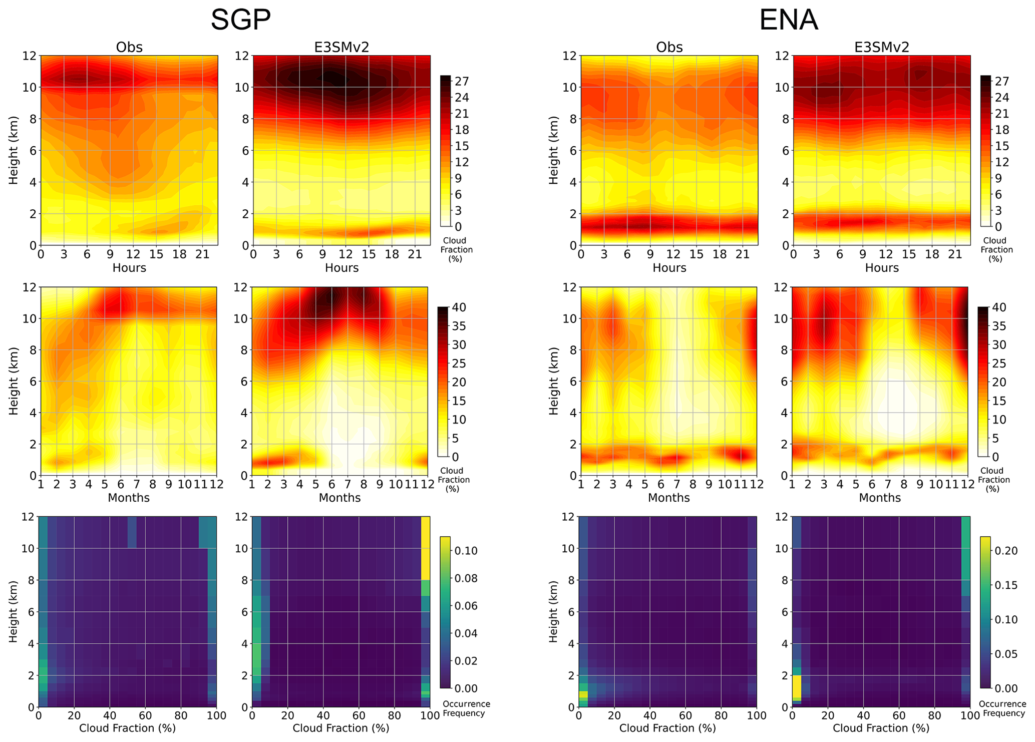
https://gmd.copernicus.org/articles/16/6355/2023/gmd-16-6355-2023-f09

Figure 9The diurnal cycle (top), seasonal cycle (middle), and occurrence frequency (bottom) of vertical cloud fraction at SGP from 2011 to 2020 (left) and ENA from 2016 to 2018 (right).

Download

Figure 9 shows the long-term diagnostics of mean diurnal cycles, seasonal cycles, and histograms of the cloud fraction by height at the SGP and ENA sites. Overall, the mean fraction of high clouds looks overestimated in E3SMv2. Similar results have been reported in many previous studies using the Community Earth System Model (CESM)–E3SM model family (e.g., Song et al., 2012; Cheng and Xu, 2013; Xu and Cheng, 2013b, a; Tang et al., 2016; Zhang et al., 2020). However, this is not an apples-to-apples comparison, as the cloud fraction in ESMs includes clouds that are optically very thin and that cannot be detected by satellite passive sensors or cloud radars. The comparison of the high-cloud fraction from simulators with the corresponding satellite observations showed that E3SM slightly underestimates high clouds over most tropical deep-convection regions (Zhang et al., 2019; Xie et al., 2018; Rasch et al., 2019). Unfortunately, a ground-based radar simulator is not available in the current model, which prevents a direct apples-to-apples comparison. Thus, caution should be taken when comparing the magnitude of the cloud fraction from direct model output and radar measurements. Here, we focus on the temporal variabilities (diurnal and seasonal cycles) and the occurrence frequency distribution of the cloud fraction, which are less relevant to the detection threshold of cloud radars.

At SGP, observations show the formation of low clouds in the afternoon and in late winter through springtime. High clouds peak overnight into the early morning and in the spring to summer, corresponding to nocturnal deep convective systems common over SGP (Tang et al., 2022b, 2021; Jiang et al., 2006). These features are reasonably well represented in E3SMv2, although low-level cloud deepening in the afternoon is not well predicted and high-level clouds peak in the late rather than early morning. At ENA, marine stratus or stratocumulus clouds occur in any month and at any time of the day, although at a lower frequency in late summer and in the afternoon. High clouds are more frequent in winter months than in summer months and occur throughout the diurnal cycle with a slight midday minimum. These features are well captured by E3SMv2. At both sites, high clouds usually occur with a high fraction (> 95 %), whereas low clouds are more likely associated with a small fraction (< 5 %) (bottom row of Fig. 9). At SGP, the high occurrence of the low-cloud fraction extends vertically up to the tropopause, representing frequently occurring deep convection. At ENA, low clouds have a smaller vertical extension but are more likely to expand to a greater fraction. E3SMv2 reproduces these cloud features in the occurrence frequency.

5.2 Multivariable relationships related to ACIs

The effective radiative forcing due to ACI processes is complex, nonlinear, and highly uncertain, despite its significant impact on climate. ACI studies are usually conducted by examining relationships between aerosols, clouds, and radiation variables that are known to interact with one another. Given so many variable combinations related to ACIs, ESMAC Diags v2 provides a framework for users to examine relationships between the variables that they choose using joint histograms, scatterplots, and heatmaps. Here, we show a few examples to assess relationships between CCN, N_d, LWP, and top-of-atmosphere (TOA) albedo. ESMAC Diags v2 calculates the layer-mean N_d from three sources: integrated vertically from native model output, retrieved using the Ndrop algorithm, and retrieved using the Nd_sat algorithm, as shown in Table 3. In this study, we only show the ACI diagnostics using native model output, as they reveal the “true” ACI relations in the model. Users can choose to use the retrieved N_d in their studies for their purposes.

The dependence of TOA albedo A on CCN number concentration for stratiform warm clouds can be decomposed (e.g., following Quaas et al., 2008) as follows:

\begin{matrix} (1) & \frac{d A}{d \ln CCN} = (\frac{\partial A}{\partial \ln N_{d}} + \frac{\partial A}{\partial \ln LWP} \frac{d \ln LWP}{d \ln N_{d}}) \frac{d \ln N_{d}}{d \ln CCN} . \end{matrix}

This allows isolation of the Twomey effect ( $\frac{\partial A}{\partial \ln N_{d}}$ ) ( $\frac{d \ln N_{d}}{d \ln CCN}$ ) and LWP adjustment ( $\frac{d \ln LWP}{d \ln N_{d}}$ ) associated with specific ACI processes. Here, we use joint histograms and heatmaps to evaluate each component, $\frac{d \ln N_{d}}{d \ln CCN}$ , $\frac{d \ln LWP}{d \ln N_{d}}$ , $\frac{\partial A}{\partial \ln N_{d}}$ , and $\frac{\partial A}{\partial \ln LWP}$ , based on long-term ground and satellite measurements at the SGP (2011–2020) and ENA (2016–2018) sites. The analysis in this section (except Fig. 11) is limited to overcast (cloud fraction > 90 %), low-level (cloud-top height < 4 km), liquid-cloud (ice water path < 0.01 mm) conditions. As there is no direct measurement of the cloud-base CCN concentration from remote sensors, the surface CCN concentration is used in this study, and only clouds that are most likely to be affected by surface conditions are examined. These clouds are identified as having a cloud-base potential temperature minus surface potential temperature that is lower than 2 K. For satellite measurements, samples with a solar zenith angle greater than 65^∘ are removed to avoid N_d retrieval biases (Grosvenor et al., 2018). The sample numbers of ground, satellite, and E3SM measurements for overcast, low-level, liquid-cloud conditions are 1766, 1217, and 6369, respectively, at SGP and 3450, 1345, and 2884, respectively, at ENA. To increase the sample size for more robust statistics, satellite retrievals and E3SM output over a 5^∘ × 5^∘ domain centered on the SGP and ENA sites are included. This increases the sample numbers of ground, satellite, and E3SM measurements to 1766, 71 942, and 15 231, respectively, at SGP and 3450, 104 260, and 28 184, respectively, at ENA. Analyses of all-sky conditions and overcast, low-level, liquid-cloud conditions for a single grid point over each site are shown in Figs. S2–S7 in the Supplement. Increasing the sample size for satellite and E3SM data does not change the overall statistics shown here.

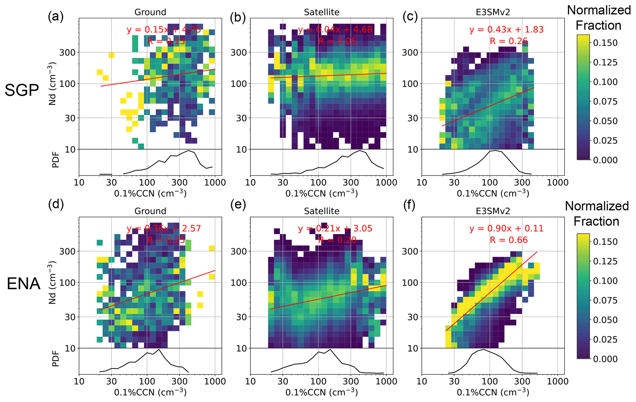
https://gmd.copernicus.org/articles/16/6355/2023/gmd-16-6355-2023-f10

Figure 10Joint histograms of the layer-mean N_d versus surface CCN number concentration at 0.1 % supersaturation, normalized within each CCN number concentration bin (PDF of CCN shown at the bottom of each panel). Samples are constrained to likely surface-coupled, overcast, low-level, liquid-cloud conditions (cloud-top height < 4 km, cloud fraction > 90 %, ice water path < 0.01 mm, and potential temperature difference between cloud base and surface < 2 K). Available samples within a 5^∘ × 5^∘ region centered on SGP (a, b, c) and ENA (d, e, f) for satellite and E3SMv2 datasets are included. Linear fits and R values are shown in red.

Download

https://gmd.copernicus.org/articles/16/6355/2023/gmd-16-6355-2023-f11

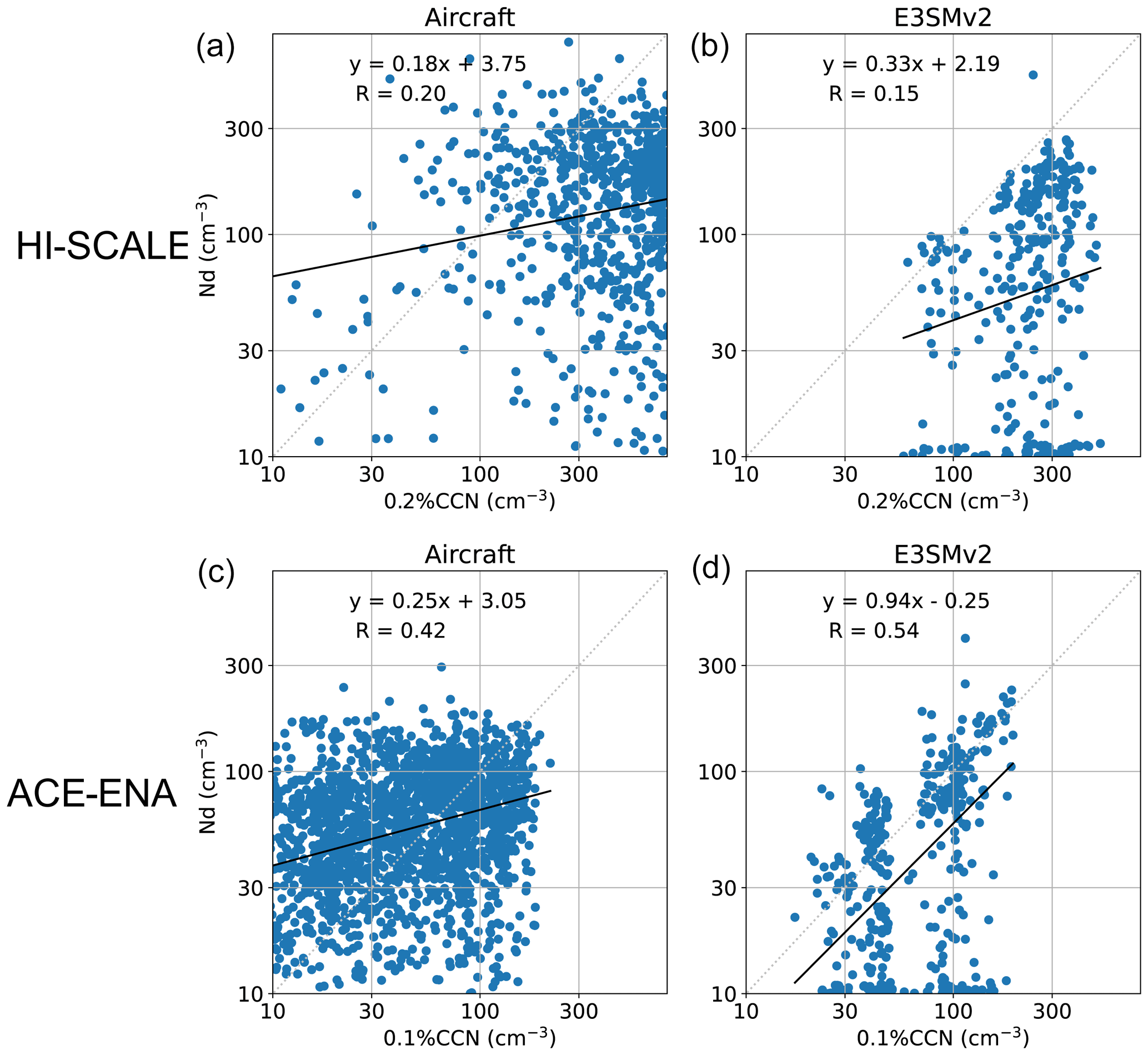
Figure 11Scatterplots of N_d versus CCN along the flight tracks from the (a, b) HI-SCALE and (c, d) ACE-ENA campaigns. Note that CCN number concentration measurements are taken at ∼ 0.2 % supersaturation for HI-SCALE and at ∼ 0.1 % supersaturation for ACE-ENA. Linear fits and R values are shown in each panel. R=0.34 (SGP) and 0.74 (ENA) for E3SMv2 if a minimum of N_d=20 cm⁻³ is applied.

Download

The change in N_d in response to a change in the surface CCN number concentration ( $\frac{d \ln N_{d}}{d \ln CCN}$ ) is heavily influenced by processes such as aerosol activation. Figure 10 shows the joint probability density function (PDF) of N_d and surface CCN number concentration at 0.1 % supersaturation, normalized within each CCN bin. Ground and satellite observations show a similar linear fit of the ln N_d–lnCCN relation, although ground-based plots have a much smaller sample number. E3SMv2 shows more sensitive N_d–CCN relationships than observations at both the SGP and ENA sites, with the relationship tighter at ENA and more scattered at SGP. As a cross-validation, Fig. 11 shows the N_d–CCN relationships from a short-term aircraft campaign during HI-SCALE and ACE-ENA. The comparison with in situ aircraft measurements confirms that E3SMv2 has a more sensitive N_d–CCN relationship than observations. These results indicate that aerosol activation in E3SMv2 may be too weak under low-CCN conditions and too strong under high-CCN conditions, which may be related to the differences in simulated and observed updraft velocity and supersaturation. Note that E3SMv2 produces a significant number of small-N_d (< 20 cm⁻³) samples (Fig. 11). This feature is reported in Golaz et al. (2022) and is partially removed by setting a minimum threshold of N_d=10 cm⁻³. However, as seen in Fig. 11, there are still a large number of N_d between 10 and 20 cm⁻³. Further investigation is underway to diagnose the causes of the abundant low-N_d values. The diagnostics shown here indicate that a more physical method should be applied to improve the simulated N_d.

The term $\frac{d \ln LWP}{d \ln N_{d}}$ is commonly interpreted as the response of the LWP to a perturbation in N_d tied to the suppression of precipitation (increased LWP) or enhancement of evaporation (decreased LWP) (e.g., Glassmeier et al., 2019). Gryspeerdt et al. (2019) showed that the satellite-retrieved LWP over the ocean increases with N_d when $N_{d} < \sim 30$ cm⁻³ and decreases when $N_{d} > \sim 30$ cm⁻³. This relation is also seen in satellite retrievals at ENA (Fig. 12) when using a higher threshold of N_d=50 cm⁻³ to perform linear fits (dashed black lines). The linear fit is insignificant for N_d<50 cm⁻³ in surface retrievals at both sites, partly due to the small sample number, and is also potentially related to drizzle contamination of the LWP. The slope of the LWP–N_d relation in satellite retrievals at SGP is positive for both N_d ranges. This is opposed to the slope from the ground retrievals and satellite retrievals at ENA. This result reveals a few difficulties with respect to LWP susceptibility studies based on observations. First, the limitations of instruments and their platforms (from space or from ground) employed in these observations as well as assumptions and simplifications in their retrieval algorithms may introduce biases and uncertainties into the retrieved cloud microphysical properties. These biases and uncertainties can be amplified when studying ACI relationships between multiple variables. Second, the robustness of ACI studies is also dependent on geographical locations and cloud types, with environmental dynamic conditions influencing the analytical outcomes. Despite our efforts to constrain meteorology and cloud situations, it is essential to acknowledge the existence of many other factors, such as cloud adiabaticity and solar zenith angle, as discussed in Varble et al. (2023), which can impact cloud susceptibility. Given these limitations and uncertainties, researchers should use caution when employing observational data to study ACI relationships.

The E3SMv2-simulated LWP–N_d relation is quite different from satellite retrievals at both sites. At SGP, it generates a positive slope for N_d<50 cm⁻³, whereas it generates a negative slope for N_d>50 cm⁻³. At ENA, it shows an opposite relation, with LWP decreases for small N_d and increases for large N_d. The overall LWP susceptibility in E3SMv2 is negative, which is consistent with observations but differs from most ESMs that produce a positive value (Quaas et al., 2009; Gryspeerdt et al., 2020). However, E3SMv2 shows a “V”-shaped LWP–N_d relation, which is the opposite of the observed “inverted-V”-shaped relation. We examined a few other oceanic regions with frequent stratus or stratocumulus clouds and saw similar behavior (not shown). This indicates possible different mechanisms of LWP susceptibility in E3SM than in observations. Our user-friendly diagnostics package allows these analyses to be routinely performed for the purpose of better understanding critical model behaviors at process- and mechanistic-levels, providing observational constraints to facilitate model development efforts.

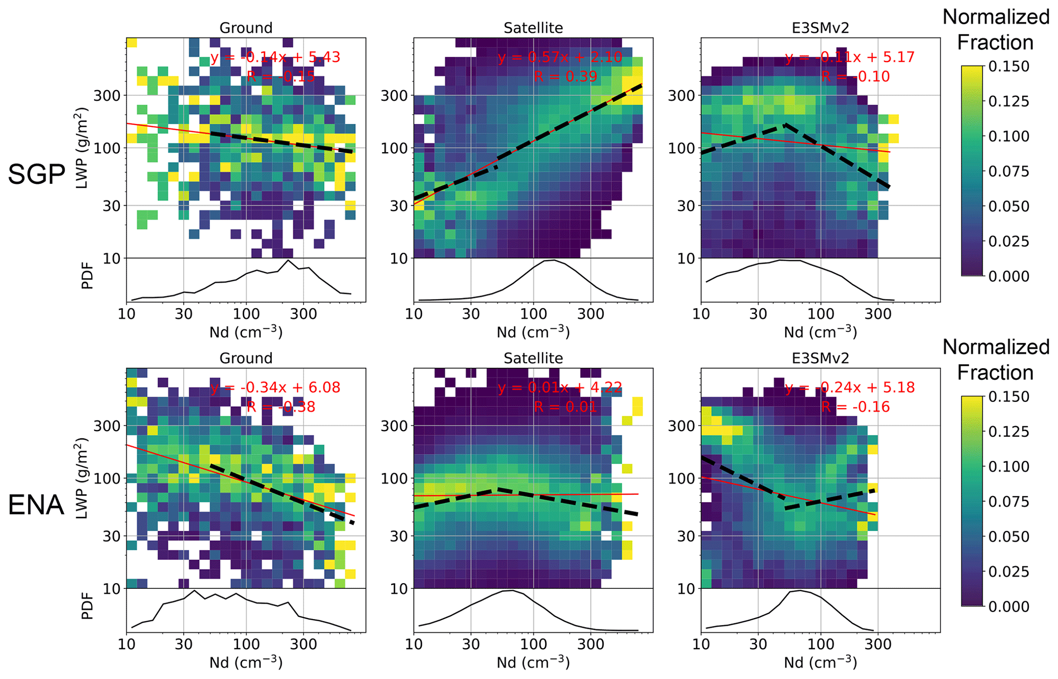
https://gmd.copernicus.org/articles/16/6355/2023/gmd-16-6355-2023-f12

Figure 12Following Fig. 10 but for the N_d bin-normalized joint histogram of LWP versus N_d. Red lines and equations are linear fits for all data samples and dashed black lines are linear fits for N_d<50 cm⁻³ and N_d>50 cm⁻³ when the fits are statistically significant (p<0.01).

Download

https://gmd.copernicus.org/articles/16/6355/2023/gmd-16-6355-2023-f13

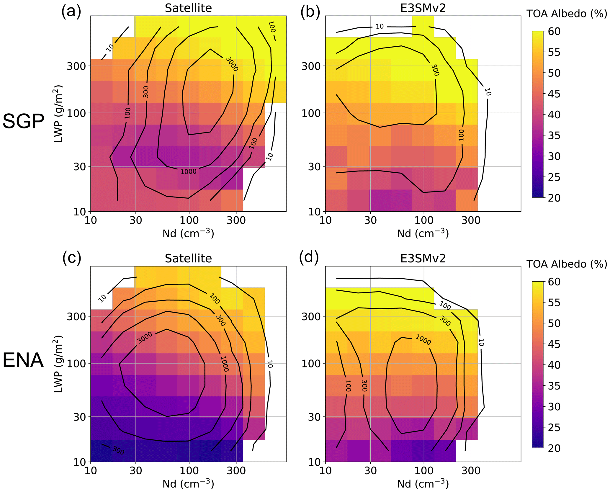
Figure 13Heatmaps of mean TOA albedo versus LWP and N_d for likely surface-coupled, overcast, low-level, liquid-cloud conditions (cloud-top height < 4 km, cloud fraction > 90 %, ice water path < 0.01 mm, and potential temperature difference between cloud base and surface < 2 K). Data include samples within a 5^∘ × 5^∘ region centered on SGP (a, b) and ENA (c, d). The valid sample numbers are shown in the black contour lines. Grids with a valid sample number < 10 are not filled. Ground data are not included, as the TOA albedo is not available.

Download

Figure 13 shows heatmaps of mean TOA albedo with respect to LWP and N_d, from which $\frac{\partial A}{\partial \ln N_{d}}$ and $\frac{\partial A}{\partial \ln LWP}$ can be derived. At both ENA and SGP, TOA albedo generally increases with increasing LWP and N_d, except at SGP when the LWP is low. The increasing albedo with a low LWP may be due to retrieval artifacts, as uncertainty becomes large when the LWP is low (e.g., < 20 g m⁻²), the solar zenith angle is high (e.g., > 55^∘), or the cloud optical depth is low (e.g., < 5) (Grosvenor et al., 2018). In most LWP–N_d bins, the TOA albedo at SGP is generally higher than at ENA, which is expected for clouds with smaller droplet sizes. An increasing TOA albedo with an increasing LWP is also seen in E3SMv2, but the dependence on N_d is weak. This can be impacted by a correlation between the solar zenith angle and N_d in E3SM simulation, as discussed in Varble et al. (2023). For a given LWP and N_d, TOA albedo is generally higher in E3SMv2 than in satellite observations, indicating that shallow clouds may be too reflective in the model, possibly due to smaller cloud R_eff (Fig. 8).

The above illustration of single-variable and multivariable diagnostics presents examples to demonstrate the capability of ESMAC Diags v2. More analyses, such as selecting other variables, performing additional data filtering or treatments, and examining ACI relationships with other variable combinations, can be conducted using user-specified settings. A detailed user guide and a collection of example scripts are included in the diagnostics package to assist users with designing customized diagnostics suited to their specific needs.

6 Summary

We developed the Earth System Model Aerosol–Cloud Diagnostics (ESMAC Diags) package to facilitate routine evaluation of aerosols, clouds, and ACIs in the US DOE E3SM model using multiple observation platforms. As an updated version of ESMAC Diags v1 (Tang et al., 2022a), which mainly prioritizes aerosol properties, this paper describes ESMAC Diags v2, which focuses on aerosols, clouds, and their interactions. In addition to the short-term field campaigns included in ESMAC Diags v1, long-term diagnostics from two permanent ARM sites (SGP and ENA, each representing continental and maritime conditions) are now conducted to provide a more robust evaluation. The newly added multivariable joint histograms, scatterplots, and heatmaps allow users to examine correlations between variables that are relevant to the study of ACIs.

Ground- and ship-based aerosol measurements are frequently impacted by local-scale emission sources, such as those from airports or ship exhaust. These local sources are not resolved by coarse-resolution ESMs, which usually represent an environmental average calculated over a region of tens to hundreds of kilometers in size. In ESMAC Diags, we used available contamination-removed aerosol data, such as those from Gallo et al. (2020) for ENA and Humphries (2020) for MARCUS, and applied data filtering for other field campaigns. The observations are harmonized into a uniform data format and temporal resolution that are comparable with ESMs. Aircraft measurements retain a higher resolution (currently 1 min) to preserve high spatiotemporal variability, although ESMs have to be downscaled for evaluation with aircraft measurements. This scale mismatch limitation must be accepted to perform evaluations in current coarse-resolution ESMs. However, as ESM grid spacing approaches a few kilometers via regional refinement (Tang et al., 2019) or global convection-permitting configurations (Caldwell et al., 2021), the scale inconsistency between models and observations is reduced. ESMAC Diags can easily adjust the preprocessing output resolution to facilitate the evaluation of high-resolution model output.

Cloud microphysical properties heavily rely on remote-sensing measurements to achieve more robust sampling, with imperfect retrieval algorithms needed to estimate these variables. Microphysical retrievals are more uncertain than typical atmospheric state measurements due to the need for many assumptions related to cloud dynamical and physical processes. We have shown (in Sect. 3) that ground- and satellite-based retrievals of N_d and R_eff are generally consistent with each other and with in situ aircraft measurements, with some systematic differences such as smaller N_d and larger R_eff values in satellite retrievals. The discrepancies between different retrievals can be larger for individual days (e.g., Fig. S1) but can be mitigated to some degree when considering broader statistics (Figs. 3, 4). The usage of multiple retrieval datasets is critical to understand the robustness of evaluation results, as the spread between different datasets indicates how robust model–observation differences are and guides the interpretations of model biases to support model development.

Finally, this paper presents a few examples of how well E3SMv2 simulates aerosols, clouds, and ACIs. We showed that ESMAC Diags can be used to target further investigation into specific parameterization components. For example, the analysis of the N_d–CCN correlation indicates that E3SMv2 may exhibit overly weak aerosol activation under low-CCN conditions and overly strong activation under high-CCN conditions; moreover, the analysis of the LWP–N_d correlation indicates that either the precipitation suppression and cloud evaporation mechanisms are not well represented or that there are other mechanisms dominating the LWP–N_d correlation in E3SMv2. These diagnostic analyses provide insights into aerosol, cloud, and ACI areas that warrant special attention in future model development efforts. As ESMs continuously improve their physical parameterizations, resolution, and numerical schemes, ESMAC Diags offers a valuable tool for systematically evaluating the performance of the newer versions of a model with respect to simulating aerosol, clouds, and ACIs.

Code availability

The current version of ESMAC Diags is publicly available through GitHub (https://github.com/eagles-project/ESMAC_diags, last access: 30 April 2023) under the new BSD license. The exact version (2.1.2) of the code used to produce the results used in this paper is archived on Zenodo (https://doi.org/10.5281/zenodo.7696871, Tang et al., 2023). The model simulation used in this paper is version 2.0 (https://doi.org/10.11578/E3SM/dc.20210927.1, E3SM Project, 2021) of E3SM.

Data availability

Measurements from the HI-SCALE, ACE-ENA, MAGIC, and MARCUS campaigns as well as the SGP and ENA sites are supported by the DOE Atmospheric Radiation Measurement (ARM) user facility and are available at https://adc.arm.gov/discovery/ (ARM Research Facility, 2023). Measurements from the CSET and SOCRATES campaigns are supported by National Science Foundation (NSF) and can be obtained from the NCAR Earth Observing Laboratory at https://doi.org/10.5065/D65Q4T96 (UCAR/NCAR – Earth Observing Laboratory, 2022a) and https://doi.org/10.5065/D6M32TM9 (UCAR/NCAR – Earth Observing Laboratory, 2022b), respectively. DOI numbers or references of individual datasets are given in Tables S1–S8. All of the preprocessed observational and model data used to produce the results used in this paper are archived on Zenodo (https://doi.org/10.5281/zenodo.7478657, Tang et al., 2022c).

Supplement

The supplement related to this article is available online at: https://doi.org/10.5194/gmd-16-6355-2023-supplement.

Author contributions

ST, JDF, and PM designed the diagnostics package; ST and ACV wrote the code and performed the analysis; PW, XD, FM, and MP processed the field campaign datasets and provided discussions on the data quality issues; KZ contributed to the model simulation; JCH contributed to the package design and setup; ST wrote the original manuscript; all authors reviewed and edited the manuscript.

Competing interests

At least one of the (co-)authors is a member of the editorial board of Geoscientific Model Development. The peer-review process was guided by an independent editor, and the authors also have no other competing interests to declare.

Disclaimer

Publisher's note: Copernicus Publications remains neutral with regard to jurisdictional claims made in the text, published maps, institutional affiliations, or any other geographical representation in this paper. While Copernicus Publications makes every effort to include appropriate place names, the final responsibility lies with the authors.

Acknowledgements

We thank the numerous instrument mentors for providing the data. This research used resources of the National Energy Research Scientific Computing Center (NERSC), a US Department of Energy Office of Science user facility operated under contract no. DE-AC02-05CH11231, using NERSC award nos. ALCC-ERCAP0016315, BER-ERCAP0015329, BER-ERCAP0018473, and BER-ERCAP0020990. Pacific Northwest National Laboratory (PNNL) is operated for DOE by Battelle Memorial Institute under contract no. DE-AC05-76RL01830.

Financial support

This study was supported by the Enabling Aerosol–cloud interactions at GLobal convection-permitting scalES (EAGLES) project (project no. 74358), funded by the US Department of Energy, Office of Science, Office of Biological and Environmental Research, Earth System Model Development (ESMD) program area.

Review statement

This paper was edited by Axel Lauer and reviewed by two anonymous referees.

References

Albrecht, B., Ghate, V., Mohrmann, J., Wood, R., Zuidema, P., Bretherton, C., Schwartz, C., Eloranta, E., Glienke, S., Donaher, S., Sarkar, M., McGibbon, J., Nugent, A. D., Shaw, R. A., Fugal, J., Minnis, P., Paliknoda, R., Lussier, L., Jensen, J., Vivekanandan, J., Ellis, S., Tsai, P., Rilling, R., Haggerty, J., Campos, T., Stell, M., Reeves, M., Beaton, S., Allison, J., Stossmeister, G., Hall, S., and Schmidt, S.: Cloud System Evolution in the Trades (CSET): Following the Evolution of Boundary Layer Cloud Systems with the NSF–NCAR GV, B. Am. Meteorol. Soc., 100, 93–121, https://doi.org/10.1175/bams-d-17-0180.1, 2019.

AMWG Diagnostic Package: https://www.cesm.ucar.edu/working_groups/Atmosphere/amwg-diagnostics-package/, last access: 2 November 2021.

ARM Research Facility: ARM Data Discovery, https://adc.arm.gov/discovery, last access: 3 March 2023.

Bennartz, R.: Global assessment of marine boundary layer cloud droplet number concentration from satellite, J. Geophys. Res.-Atmos., 112, D02201, https://doi.org/10.1029/2006JD007547, 2007.

Caldwell, P. M., Terai, C. R., Hillman, B., Keen, N. D., Bogenschutz, P., Lin, W., Beydoun, H., Taylor, M., Bertagna, L., Bradley, A. M., Clevenger, T. C., Donahue, A. S., Eldred, C., Foucar, J., Golaz, J.-C., Guba, O., Jacob, R., Johnson, J., Krishna, J., Liu, W., Pressel, K., Salinger, A. G., Singh, B., Steyer, A., Ullrich, P., Wu, D., Yuan, X., Shpund, J., Ma, H.-Y., and Zender, C. S.: Convection-Permitting Simulations With the E3SM Global Atmosphere Model, J. Adv. Model. Earth Sy., 13, e2021MS002544, https://doi.org/10.1029/2021MS002544, 2021.

Cheng, A. and Xu, K.-M.: Evaluating Low-Cloud Simulation from an Upgraded Multiscale Modeling Framework Model. Part III: Tropical and Subtropical Cloud Transitions over the Northern Pacific, J. Climate, 26, 5761–5781, https://doi.org/10.1175/JCLI-D-12-00650.1, 2013.

Choudhury, G. and Tesche, M.: Estimating cloud condensation nuclei concentrations from CALIPSO lidar measurements, Atmos. Meas. Tech., 15, 639–654, https://doi.org/10.5194/amt-15-639-2022, 2022.

E3SM Diagnostics: https://e3sm.org/resources/tools/diagnostic-tools/e3sm-diagnostics/, last access: 2 November 2021.

E3SM Project: Energy Exascale Earth System Model v2.0, Computer Software, DOE [code], https://doi.org/10.11578/E3SM/dc.20210927.1, 2021.

Eyring, V., Righi, M., Lauer, A., Evaldsson, M., Wenzel, S., Jones, C., Anav, A., Andrews, O., Cionni, I., Davin, E. L., Deser, C., Ehbrecht, C., Friedlingstein, P., Gleckler, P., Gottschaldt, K.-D., Hagemann, S., Juckes, M., Kindermann, S., Krasting, J., Kunert, D., Levine, R., Loew, A., Mäkelä, J., Martin, G., Mason, E., Phillips, A. S., Read, S., Rio, C., Roehrig, R., Senftleben, D., Sterl, A., van Ulft, L. H., Walton, J., Wang, S., and Williams, K. D.: ESMValTool (v1.0) – a community diagnostic and performance metrics tool for routine evaluation of Earth system models in CMIP, Geosci. Model Dev., 9, 1747–1802, https://doi.org/10.5194/gmd-9-1747-2016, 2016.

Fast, J. D., Berg, L. K., Alexander, L., Bell, D., D'Ambro, E., Hubbe, J., Kuang, C., Liu, J., Long, C., Matthews, A., Mei, F., Newsom, R., Pekour, M., Pinterich, T., Schmid, B., Schobesberger, S., Shilling, J., Smith, J. N., Springston, S., Suski, K., Thornton, J. A., Tomlinson, J., Wang, J., Xiao, H., and Zelenyuk, A.: Overview of the HI-SCALE Field Campaign: A New Perspective on Shallow Convective Clouds, B. Am. Meteorol. Soc., 100, 821–840, https://doi.org/10.1175/bams-d-18-0030.1, 2019.

Gallo, F., Uin, J., Springston, S., Wang, J., Zheng, G., Kuang, C., Wood, R., Azevedo, E. B., McComiskey, A., Mei, F., Theisen, A., Kyrouac, J., and Aiken, A. C.: Identifying a regional aerosol baseline in the eastern North Atlantic using collocated measurements and a mathematical algorithm to mask high-submicron-number-concentration aerosol events, Atmos. Chem. Phys., 20, 7553–7573, https://doi.org/10.5194/acp-20-7553-2020, 2020.

Gelaro, R., McCarty, W., Suarez, M. J., Todling, R., Molod, A., Takacs, L., Randles, C., Darmenov, A., Bosilovich, M. G., Reichle, R., Wargan, K., Coy, L., Cullather, R., Draper, C., Akella, S., Buchard, V., Conaty, A., da Silva, A., Gu, W., Kim, G. K., Koster, R., Lucchesi, R., Merkova, D., Nielsen, J. E., Partyka, G., Pawson, S., Putman, W., Rienecker, M., Schubert, S. D., Sienkiewicz, M., and Zhao, B.: The Modern-Era Retrospective Analysis for Research and Applications, Version 2 (MERRA-2), J. Climate, 30, 5419–5454, https://doi.org/10.1175/JCLI-D-16-0758.1, 2017.

Glassmeier, F., Hoffmann, F., Johnson, J. S., Yamaguchi, T., Carslaw, K. S., and Feingold, G.: An emulator approach to stratocumulus susceptibility, Atmos. Chem. Phys., 19, 10191–10203, https://doi.org/10.5194/acp-19-10191-2019, 2019.

Gleckler, P. J., Doutriaux, C., Durack, P. J., Taylor, K. E., Zhang, Y., Williams, D. N., Mason, E., and Servonnat, J.: A more powerful reality test for climate models, Eos T. Am. Geophys. Un., 97, https://doi.org/10.1029/2016EO051663, 2016.

Golaz, J.-C., Caldwell, P. M., Van Roekel, L. P., Petersen, M. R., Tang, Q., Wolfe, J. D., Abeshu, G., Anantharaj, V., Asay-Davis, X. S., Bader, D. C., Baldwin, S. A., Bisht, G., Bogenschutz, P. A., Branstetter, M., Brunke, M. A., Brus, S. R., Burrows, S. M., Cameron-Smith, P. J., Donahue, A. S., Deakin, M., Easter, R. C., Evans, K. J., Feng, Y., Flanner, M., Foucar, J. G., Fyke, J. G., Griffin, B. M., Hannay, C., Harrop, B. E., Hoffman, M. J., Hunke, E. C., Jacob, R. L., Jacobsen, D. W., Jeffery, N., Jones, P. W., Keen, N. D., Klein, S. A., Larson, V. E., Leung, L. R., Li, H.-Y., Lin, W., Lipscomb, W. H., Ma, P.-L., Mahajan, S., Maltrud, M. E., Mametjanov, A., McClean, J. L., McCoy, R. B., Neale, R. B., Price, S. F., Qian, Y., Rasch, P. J., Reeves Eyre, J. E. J., Riley, W. J., Ringler, T. D., Roberts, A. F., Roesler, E. L., Salinger, A. G., Shaheen, Z., Shi, X., Singh, B., Tang, J., Taylor, M. A., Thornton, P. E., Turner, A. K., Veneziani, M., Wan, H., Wang, H., Wang, S., Williams, D. N., Wolfram, P. J., Worley, P. H., Xie, S., Yang, Y., Yoon, J.-H., Zelinka, M. D., Zender, C. S., Zeng, X., Zhang, C., Zhang, K., Zhang, Y., Zheng, X., Zhou, T., and Zhu, Q.: The DOE E3SM Coupled Model Version 1: Overview and Evaluation at Standard Resolution, J. Adv. Model. Earth Sy., 11, 2089–2129, https://doi.org/10.1029/2018ms001603, 2019.

Golaz, J.-C., Van Roekel, L. P., Zheng, X., Roberts, A. F., Wolfe, J. D., Lin, W., Bradley, A. M., Tang, Q., Maltrud, M. E., Forsyth, R. M., Zhang, C., Zhou, T., Zhang, K., Zender, C. S., Wu, M., Wang, H., Turner, A. K., Singh, B., Richter, J. H., Qin, Y., Petersen, M. R., Mametjanov, A., Ma, P.-L., Larson, V. E., Krishna, J., Keen, N. D., Jeffery, N., Hunke, E. C., Hannah, W. M., Guba, O., Griffin, B. M., Feng, Y., Engwirda, D., Di Vittorio, A. V., Dang, C., Conlon, L. M., Chen, C.-C.-J., Brunke, M. A., Bisht, G., Benedict, J. J., Asay-Davis, X. S., Zhang, Y., Zhang, M., Zeng, X., Xie, S., Wolfram, P. J., Vo, T., Veneziani, M., Tesfa, T. K., Sreepathi, S., Salinger, A. G., Jack Reeves Eyre, J. E., Prather, M. J., Mahajan, S., Li, Q., Jones, P. W., Jacob, R. L., Huebler, G. W., Huang, X., Hillman, B. R., Harrop, B. E., Foucar, J. G., Fang, Y., Comeau, D. S., Caldwell, P. M., Bartoletti, T., Balaguru, K., Taylor, M. A., McCoy, R. B., Leung, L. R., and Bader, D. C.: The DOE E3SM Model Version 2: Overview of the physical model and initial model evaluation, J. Adv. Model. Earth Sy., 14, e2022MS003156, https://doi.org/10.1029/2022MS003156, 2022.

Grosvenor, D. P., Sourdeval, O., Zuidema, P., Ackerman, A., Alexandrov, M. D., Bennartz, R., Boers, R., Cairns, B., Chiu, J. C., Christensen, M., Deneke, H., Diamond, M., Feingold, G., Fridlind, A., Hünerbein, A., Knist, C., Kollias, P., Marshak, A., McCoy, D., Merk, D., Painemal, D., Rausch, J., Rosenfeld, D., Russchenberg, H., Seifert, P., Sinclair, K., Stier, P., van Diedenhoven, B., Wendisch, M., Werner, F., Wood, R., Zhang, Z., and Quaas, J.: Remote Sensing of Droplet Number Concentration in Warm Clouds: A Review of the Current State of Knowledge and Perspectives, Rev. Geophys., 56, 409–453, https://doi.org/10.1029/2017RG000593, 2018.

Gryspeerdt, E., Goren, T., Sourdeval, O., Quaas, J., Mülmenstädt, J., Dipu, S., Unglaub, C., Gettelman, A., and Christensen, M.: Constraining the aerosol influence on cloud liquid water path, Atmos. Chem. Phys., 19, 5331–5347, https://doi.org/10.5194/acp-19-5331-2019, 2019.

Gryspeerdt, E., Mülmenstädt, J., Gettelman, A., Malavelle, F. F., Morrison, H., Neubauer, D., Partridge, D. G., Stier, P., Takemura, T., Wang, H., Wang, M., and Zhang, K.: Surprising similarities in model and observational aerosol radiative forcing estimates, Atmos. Chem. Phys., 20, 613–623, https://doi.org/10.5194/acp-20-613-2020, 2020.

Humphries, R.: MARCUS ARM CN and CCN data reprocessed to remove ship exhaust influence (v2), Csiro [data set], https://doi.org/10.25919/ezp0-em87, 2020.

Humphries, R. S., McRobert, I. M., Ponsonby, W. A., Ward, J. P., Keywood, M. D., Loh, Z. M., Krummel, P. B., and Harnwell, J.: Identification of platform exhaust on the RV Investigator, Atmos. Meas. Tech., 12, 3019–3038, https://doi.org/10.5194/amt-12-3019-2019, 2019.

IPCC: Climate Change 2021: The Physical Science Basis. Contribution of Working Group I to the Sixth Assessment Report of the Intergovernmental Panel on Climate Change, Cambridge University Press, Cambridge, United Kingdom and New York, NY, USA, 2391 pp., https://doi.org/10.1017/9781009157896, 2021.

Jiang, X., Lau, N.-C., and Klein, S. A.: Role of eastward propagating convection systems in the diurnal cycle and seasonal mean of summertime rainfall over the U.S. Great Plains, Geophys. Res. Lett., 33, L19809, https://doi.org/10.1029/2006gl027022, 2006.

Lewis, E. R. and Teixeira, J.: Dispelling clouds of uncertainty, Eos T. Am. Geophys. Un., 96, https://doi.org/10.1029/2015eo031303, 2015.

Lim, K.-S. S., Riihimaki, L., Comstock, J. M., Schmid, B., Sivaraman, C., Shi, Y., and McFarquhar, G. M.: Evaluation of long-term surface-retrieved cloud droplet number concentration with in situ aircraft observations, J. Geophys. Res.-Atmos., 121, 2318–2331, https://doi.org/10.1002/2015JD024082, 2016.

Ma, P.-L., Harrop, B. E., Larson, V. E., Neale, R. B., Gettelman, A., Morrison, H., Wang, H., Zhang, K., Klein, S. A., Zelinka, M. D., Zhang, Y., Qian, Y., Yoon, J.-H., Jones, C. R., Huang, M., Tai, S.-L., Singh, B., Bogenschutz, P. A., Zheng, X., Lin, W., Quaas, J., Chepfer, H., Brunke, M. A., Zeng, X., Mülmenstädt, J., Hagos, S., Zhang, Z., Song, H., Liu, X., Pritchard, M. S., Wan, H., Wang, J., Tang, Q., Caldwell, P. M., Fan, J., Berg, L. K., Fast, J. D., Taylor, M. A., Golaz, J.-C., Xie, S., Rasch, P. J., and Leung, L. R.: Better calibration of cloud parameterizations and subgrid effects increases the fidelity of the E3SM Atmosphere Model version 1, Geosci. Model Dev., 15, 2881–2916, https://doi.org/10.5194/gmd-15-2881-2022, 2022.

Maloney, E. D., Gettelman, A., Ming, Y., Neelin, J. D., Barrie, D., Mariotti, A., Chen, C. C., Coleman, D. R. B., Kuo, Y.-H., Singh, B., Annamalai, H., Berg, A., Booth, J. F., Camargo, S. J., Dai, A., Gonzalez, A., Hafner, J., Jiang, X., Jing, X., Kim, D., Kumar, A., Moon, Y., Naud, C. M., Sobel, A. H., Suzuki, K., Wang, F., Wang, J., Wing, A. A., Xu, X., and Zhao, M.: Process-Oriented Evaluation of Climate and Weather Forecasting Models, B. Am. Meteorol. Soc., 100, 1665–1686, https://doi.org/10.1175/bams-d-18-0042.1, 2019.

McFarquhar, G. M., Bretherton, C. S., Marchand, R., Protat, A., DeMott, P. J., Alexander, S. P., Roberts, G. C., Twohy, C. H., Toohey, D., Siems, S., Huang, Y., Wood, R., Rauber, R. M., Lasher-Trapp, S., Jensen, J., Stith, J. L., Mace, J., Um, J., Järvinen, E., Schnaiter, M., Gettelman, A., Sanchez, K. J., McCluskey, C. S., Russell, L. M., McCoy, I. L., Atlas, R. L., Bardeen, C. G., Moore, K. A., Hill, T. C. J., Humphries, R. S., Keywood, M. D., Ristovski, Z., Cravigan, L., Schofield, R., Fairall, C., Mallet, M. D., Kreidenweis, S. M., Rainwater, B., D'Alessandro, J., Wang, Y., Wu, W., Saliba, G., Levin, E. J. T., Ding, S., Lang, F., Truong, S. C. H., Wolff, C., Haggerty, J., Harvey, M. J., Klekociuk, A. R., and McDonald, A.: Observations of Clouds, Aerosols, Precipitation, and Surface Radiation over the Southern Ocean: An Overview of CAPRICORN, MARCUS, MICRE, and SOCRATES, B. Am. Meteorol. Soc., 102, E894–E928, https://doi.org/10.1175/bams-d-20-0132.1, 2021.

Min, Q. and Harrison, L. C.: Cloud properties derived from surface MFRSR measurements and comparison with GOES results at the ARM SGP Site, Geophys. Res. Lett., 23, 1641–1644, https://doi.org/10.1029/96GL01488, 1996.

Minnis, P., Nguyen, L., Palikonda, R., Heck, P. W., Spangenberg, D. A., Doelling, D. R., Ayers, J. K., Smith, J. W. L., Khaiyer, M. M., Trepte, Q. Z., Avey, L. A., Chang, F.-L., Yost, C. R., Chee, T. L., and Szedung, S.-M.: Near-real time cloud retrievals from operational and research meteorological satellites, Proc. SPIE Europe Remote Sens., Cardiff, Wales, UK, 15–18 September, 710703, https://doi.org/10.1117/12.800344, 2008.

Minnis, P., Sun-Mack, S., Young, D. F., Heck, P. W., Garber, D. P., Chen, Y., Spangenberg, D. A., Arduini, R. F., Trepte, Q. Z., Smith, W. L., Ayers, J. K., Gibson, S. C., Miller, W. F., Hong, G., Chakrapani, V., Takano, Y., Liou, K. N., Xie, Y., and Yang, P.: CERES Edition-2 Cloud Property Retrievals Using TRMM VIRS and Terra and Aqua MODIS Data – Part I: Algorithms, IEEE T. Geosci. Remote, 49, 4374–4400, https://doi.org/10.1109/TGRS.2011.2144601, 2011.

Myhre, G., Samset, B. H., Schulz, M., Balkanski, Y., Bauer, S., Berntsen, T. K., Bian, H., Bellouin, N., Chin, M., Diehl, T., Easter, R. C., Feichter, J., Ghan, S. J., Hauglustaine, D., Iversen, T., Kinne, S., Kirkevåg, A., Lamarque, J.-F., Lin, G., Liu, X., Lund, M. T., Luo, G., Ma, X., van Noije, T., Penner, J. E., Rasch, P. J., Ruiz, A., Seland, Ø., Skeie, R. B., Stier, P., Takemura, T., Tsigaridis, K., Wang, P., Wang, Z., Xu, L., Yu, H., Yu, F., Yoon, J.-H., Zhang, K., Zhang, H., and Zhou, C.: Radiative forcing of the direct aerosol effect from AeroCom Phase II simulations, Atmos. Chem. Phys., 13, 1853–1877, https://doi.org/10.5194/acp-13-1853-2013, 2013.

NETCDF: Introduction and Overview: https://www.unidata.ucar.edu/software/netcdf/docs/index.html, last access: 12 November 2022.

Quaas, J., Boucher, O., Bellouin, N., and Kinne, S.: Satellite-based estimate of the direct and indirect aerosol climate forcing, J. Geophys. Res.-Atmos., 113, D05204, https://doi.org/10.1029/2007JD008962, 2008.

Quaas, J., Ming, Y., Menon, S., Takemura, T., Wang, M., Penner, J. E., Gettelman, A., Lohmann, U., Bellouin, N., Boucher, O., Sayer, A. M., Thomas, G. E., McComiskey, A., Feingold, G., Hoose, C., Kristjánsson, J. E., Liu, X., Balkanski, Y., Donner, L. J., Ginoux, P. A., Stier, P., Grandey, B., Feichter, J., Sednev, I., Bauer, S. E., Koch, D., Grainger, R. G., Kirkevåg, A., Iversen, T., Seland, Ø., Easter, R., Ghan, S. J., Rasch, P. J., Morrison, H., Lamarque, J.-F., Iacono, M. J., Kinne, S., and Schulz, M.: Aerosol indirect effects – general circulation model intercomparison and evaluation with satellite data, Atmos. Chem. Phys., 9, 8697–8717, https://doi.org/10.5194/acp-9-8697-2009, 2009.

Rasch, P. J., Xie, S., Ma, P.-L., Lin, W., Wang, H., Tang, Q., Burrows, S. M., Caldwell, P., Zhang, K., Easter, R. C., Cameron-Smith, P., Singh, B., Wan, H., Golaz, J.-C., Harrop, B. E., Roesler, E., Bacmeister, J., Larson, V. E., Evans, K. J., Qian, Y., Taylor, M., Leung, L. R., Zhang, Y., Brent, L., Branstetter, M., Hannay, C., Mahajan, S., Mametjanov, A., Neale, R., Richter, J. H., Yoon, J.-H., Zender, C. S., Bader, D., Flanner, M., Foucar, J. G., Jacob, R., Keen, N., Klein, S. A., Liu, X., Salinger, A. G., Shrivastava, M., and Yang, Y.: An Overview of the Atmospheric Component of the Energy Exascale Earth System Model, J. Adv. Model. Earth Sy., 11, 2377–2411, https://doi.org/10.1029/2019ms001629, 2019.

Reddington, C. L., Carslaw, K. S., Stier, P., Schutgens, N., Coe, H., Liu, D., Allan, J., Browse, J., Pringle, K. J., Lee, L. A., Yoshioka, M., Johnson, J. S., Regayre, L. A., Spracklen, D. V., Mann, G. W., Clarke, A., Hermann, M., Henning, S., Wex, H., Kristensen, T. B., Leaitch, W. R., Pöschl, U., Rose, D., Andreae, M. O., Schmale, J., Kondo, Y., Oshima, N., Schwarz, J. P., Nenes, A., Anderson, B., Roberts, G. C., Snider, J. R., Leck, C., Quinn, P. K., Chi, X., Ding, A., Jimenez, J. L., and Zhang, Q.: The Global Aerosol Synthesis and Science Project (GASSP): Measurements and Modeling to Reduce Uncertainty, B. Am. Meteorol. Soc., 98, 1857–1877, https://doi.org/10.1175/bams-d-15-00317.1, 2017.

Riihimaki, L., McFarlane, S., and Sivaraman, C.: Droplet Number Concentration Value-Added Product, ARM Research Facility, https://doi.org/10.2172/1237963, 2021.

Schulz, M., Textor, C., Kinne, S., Balkanski, Y., Bauer, S., Berntsen, T., Berglen, T., Boucher, O., Dentener, F., Guibert, S., Isaksen, I. S. A., Iversen, T., Koch, D., Kirkevåg, A., Liu, X., Montanaro, V., Myhre, G., Penner, J. E., Pitari, G., Reddy, S., Seland, Ø., Stier, P., and Takemura, T.: Radiative forcing by aerosols as derived from the AeroCom present-day and pre-industrial simulations, Atmos. Chem. Phys., 6, 5225–5246, https://doi.org/10.5194/acp-6-5225-2006, 2006.

Song, X., Zhang, G. J., and Li, J. L. F.: Evaluation of Microphysics Parameterization for Convective Clouds in the NCAR Community Atmosphere Model CAM5, J. Climate, 25, 8568–8590, https://doi.org/10.1175/JCLI-D-11-00563.1, 2012.

Sun, J., Zhang, K., Wan, H., Ma, P.-L., Tang, Q., and Zhang, S.: Impact of Nudging Strategy on the Climate Representativeness and Hindcast Skill of Constrained EAMv1 Simulations, J. Adv. Model. Earth Sy., 11, 3911–3933, https://doi.org/10.1029/2019MS001831, 2019.

Tang, Q., Klein, S. A., Xie, S., Lin, W., Golaz, J.-C., Roesler, E. L., Taylor, M. A., Rasch, P. J., Bader, D. C., Berg, L. K., Caldwell, P., Giangrande, S. E., Neale, R. B., Qian, Y., Riihimaki, L. D., Zender, C. S., Zhang, Y., and Zheng, X.: Regionally refined test bed in E3SM atmosphere model version 1 (EAMv1) and applications for high-resolution modeling, Geosci. Model Dev., 12, 2679–2706, https://doi.org/10.5194/gmd-12-2679-2019, 2019.

Tang, S., Zhang, M., and Xie, S.: An ensemble constrained variational analysis of atmospheric forcing data and its application to evaluate clouds in CAM5, J. Geophys. Res.-Atmos., 121, 33–48, https://doi.org/10.1002/2015JD024167, 2016.

Tang, S., Gleckler, P., Xie, S., Lee, J., Ahn, M.-S., Covey, C., and Zhang, C.: Evaluating the Diurnal and Semidiurnal Cycle of Precipitation in CMIP6 Models Using Satellite- and Ground-Based Observations, J. Climate, 34, 3189–3210, https://doi.org/10.1175/jcli-d-20-0639.1, 2021.

Tang, S., Fast, J. D., Zhang, K., Hardin, J. C., Varble, A. C., Shilling, J. E., Mei, F., Zawadowicz, M. A., and Ma, P.-L.: Earth System Model Aerosol–Cloud Diagnostics (ESMAC Diags) package, version 1: assessing E3SM aerosol predictions using aircraft, ship, and surface measurements, Geosci. Model Dev., 15, 4055–4076, https://doi.org/10.5194/gmd-15-4055-2022, 2022a.

Tang, S., Xie, S., Guo, Z., Hong, S.-Y., Khouider, B., Klocke, D., Köhler, M., Koo, M.-S., Krishna, P. M., Larson, V. E., Park, S., Vaillancourt, P. A., Wang, Y.-C., Yang, J., Daleu, C. L., Homeyer, C. R., Jones, T. R., Malap, N., Neggers, R., Prabhakaran, T., Ramirez, E., Schumacher, C., Tao, C., Bechtold, P., Ma, H.-Y., Neelin, J. D., and Zeng, X.: Long-term single-column model intercomparison of diurnal cycle of precipitation over midlatitude and tropical land, Q. J. Roy. Meteor. Soc., 148, 641–669, https://doi.org/10.1002/qj.4222, 2022b.

Tang, S., Fast, J. D., Varble, A. C., Hardin, J. C., and Ma, P.-L.: ESMAC Diags data (2.1), Zenodo [data set], https://doi.org/10.5281/zenodo.7478657, 2022c.

Tang, S., Varble, A. C., Fast, J. D., Hardin, J. C., and Ma, P.-L.: ESMAC Diags code (2.1.2), Zenodo [code], https://doi.org/10.5281/zenodo.7696871, 2023.

Turner, D. D., Lo, C., Min, Q., Zhang, D., and Gaustad, K.: Cloud Optical Properties from the Multifilter Shadowband Radiometer (MFRSRCLDOD): An ARM Value-Added Product, ARM Research FacilityDOE/SC-ARM-TR-047, 2021.

UCAR/NCAR – Earth Observing Laboratory: CSET: Low Rate (LRT – 1 sps) Navigation, State Parameter, and Microphysics Flight-Level Data. Version 1.4, UCAR/NCAR – Earth Observing Laboratory [data set], https://doi.org/10.5065/D65Q4T96, 2022a.

UCAR/NCAR – Earth Observing Laboratory: SOCRATES: Low Rate (LRT – 1 sps) Navigation, State Parameter, and Microphysics Flight-Level Data. Version 1.4, UCAR/NCAR – Earth Observing Laboratory [data set], https://doi.org/10.5065/D6M32TM9, 2022b.

Varble, A. C., Ma, P.-L., Christensen, M. W., Mülmenstädt, J., Tang, S., and Fast, J.: Evaluation of Liquid Cloud Albedo Susceptibility in E3SM Using Coupled Eastern North Atlantic Surface and Satellite Retrievals, EGUsphere [preprint], https://doi.org/10.5194/egusphere-2023-998, 2023.

Wang, J., Wood, R., Jensen, M. P., Chiu, J. C., Liu, Y., Lamer, K., Desai, N., Giangrande, S. E., Knopf, D. A., Kollias, P., Laskin, A., Liu, X., Lu, C., Mechem, D., Mei, F., Starzec, M., Tomlinson, J., Wang, Y., Yum, S. S., Zheng, G., Aiken, A. C., Azevedo, E. B., Blanchard, Y., China, S., Dong, X., Gallo, F., Gao, S., Ghate, V. P., Glienke, S., Goldberger, L., Hardin, J. C., Kuang, C., Luke, E. P., Matthews, A. A., Miller, M. A., Moffet, R., Pekour, M., Schmid, B., Sedlacek, A. J., Shaw, R. A., Shilling, J. E., Sullivan, A., Suski, K., Veghte, D. P., Weber, R., Wyant, M., Yeom, J., Zawadowicz, M., and Zhang, Z.: Aerosol and Cloud Experiments in the Eastern North Atlantic (ACE-ENA), B. Am. Meteorol. Soc., 103, E619–E641, https://doi.org/10.1175/bams-d-19-0220.1, 2022.

Watson-Parris, D., Schutgens, N., Reddington, C., Pringle, K. J., Liu, D., Allan, J. D., Coe, H., Carslaw, K. S., and Stier, P.: In situ constraints on the vertical distribution of global aerosol, Atmos. Chem. Phys., 19, 11765–11790, https://doi.org/10.5194/acp-19-11765-2019, 2019.

Wu, P., Dong, X., Xi, B., Tian, J., and Ward, D. M.: Profiles of MBL Cloud and Drizzle Microphysical Properties Retrieved From Ground-Based Observations and Validated by Aircraft In Situ Measurements Over the Azores, J. Geophys. Res.-Atmos., 125, e2019JD032205, https://doi.org/10.1029/2019JD032205, 2020.

Xie, S., Lin, W., Rasch, P. J., Ma, P.-L., Neale, R., Larson, V. E., Qian, Y., Bogenschutz, P. A., Caldwell, P., Cameron-Smith, P., Golaz, J.-C., Mahajan, S., Singh, B., Tang, Q., Wang, H., Yoon, J.-H., Zhang, K., and Zhang, Y.: Understanding Cloud and Convective Characteristics in Version 1 of the E3SM Atmosphere Model, J. Adv. Model. Earth Sy., 10, 2618–2644, https://doi.org/10.1029/2018MS001350, 2018.

Xu, K.-M. and Cheng, A.: Evaluating Low-Cloud Simulation from an Upgraded Multiscale Modeling Framework Model. Part II: Seasonal Variations over the Eastern Pacific, J. Climate, 26, 5741–5760, https://doi.org/10.1175/JCLI-D-12-00276.1, 2013a.

Xu, K.-M. and Cheng, A.: Evaluating Low-Cloud Simulation from an Upgraded Multiscale Modeling Framework Model. Part I: Sensitivity to Spatial Resolution and Climatology, J. Climate, 26, 5717–5740, https://doi.org/10.1175/JCLI-D-12-00200.1, 2013b.

Zhang, C., Xie, S., Tao, C., Tang, S., Emmenegger, T., Neelin, J. D., Schiro, K. A., Lin, W., and Shaheen, Z.: The ARM Data-Oriented Metrics and Diagnostics Package for Climate Models: A New Tool for Evaluating Climate Models with Field Data, B. Am. Meteorol. Soc., 101, E1619–E1627, https://doi.org/10.1175/bams-d-19-0282.1, 2020.

Zhang, S., Zhang, K., Wan, H., and Sun, J.: Further improvement and evaluation of nudging in the E3SM Atmosphere Model version 1 (EAMv1): simulations of the mean climate, weather events, and anthropogenic aerosol effects, Geosci. Model Dev., 15, 6787–6816, https://doi.org/10.5194/gmd-15-6787-2022, 2022.

Zhang, Y., Xie, S., Lin, W., Klein, S. A., Zelinka, M., Ma, P.-L., Rasch, P. J., Qian, Y., Tang, Q., and Ma, H.-Y.: Evaluation of Clouds in Version 1 of the E3SM Atmosphere Model With Satellite Simulators, J. Adv. Model. Earth Sy., 11, 1253–1268, https://doi.org/10.1029/2018MS001562, 2019.

Zhou, X., Kollias, P., and Lewis, E. R.: Clouds, Precipitation, and Marine Boundary Layer Structure during the MAGIC Field Campaign, J. Climate, 28, 2420–2442, https://doi.org/10.1175/jcli-d-14-00320.1, 2015.

Articles

Short summary

To assess the ability of Earth system model (ESM) predictions, we developed a tool called ESMAC Diags to understand how aerosols, clouds, and aerosol–cloud interactions are represented in ESMs. This paper describes its version 2 functionality. We compared the model predictions with measurements taken by planes, ships, satellites, and ground instruments over four regions across the world. Results show that this new tool can help identify model problems and guide future development of ESMs.