Articles | Volume 16, issue 15

https://doi.org/10.5194/gmd-16-4427-2023

Articles | Volume 16, issue 15

Methods for assessment of models

| Highlight paper

02 Aug 2023

Methods for assessment of models | Highlight paper |

| 02 Aug 2023

The three-dimensional structure of fronts in mid-latitude weather systems in numerical weather prediction models

Andreas A. Beckert, Lea Eisenstein, Annika Oertel, Tim Hewson, George C. Craig, and Marc Rautenhaus

Video abstract

Abstract

Atmospheric fronts are a widely used conceptual model in meteorology, most encountered as two-dimensional (2-D) front lines on surface analysis charts. The three-dimensional (3-D) dynamical structure of fronts has been studied in the literature by means of “standard” 2-D maps and cross-sections and is commonly sketched in 3-D illustrations of idealized weather systems in atmospheric science textbooks. However, only recently has the feasibility of the objective detection and visual analysis of 3-D frontal structures and their dynamics within numerical weather prediction (NWP) data been proposed, and such approaches are not yet widely known in the atmospheric science community. In this article, we investigate the benefit of objective 3-D front detection for case studies of extra-tropical cyclones and for comparison of frontal structures between different NWP models. We build on a recent gradient-based detection approach, combined with modern 3-D interactive visual analysis techniques, and adapt it to handle data from state-of-the-art NWP models including those run at convection-permitting kilometre-scale resolution. The parameters of the detection method (including data smoothing and threshold parameters) are evaluated to yield physically meaningful structures. We illustrate the benefit of the method by presenting two case studies of frontal dynamics within mid-latitude cyclones. Examples include joint interactive visual analysis of 3-D fronts and warm conveyor belt (WCB) trajectories, as well as identification of the 3-D frontal structures characterizing the different stages of a Shapiro–Keyser cyclogenesis event. The 3-D frontal structures show agreement with 2-D fronts from surface analysis charts and augment the surface charts by providing additional pertinent information in the vertical dimension. A second application illustrates the relation between convection and 3-D cold-front structure by comparing data from simulations with parameterized and explicit convection. Finally, we consider “secondary fronts” that commonly appear in UK Met Office surface analysis charts. Examination of a case study shows that for this event the secondary front is not a temperature-dominated but a humidity-dominated feature. We argue that the presented approach has great potential to be beneficial for more complex studies of atmospheric dynamics and for operational weather forecasting.

Download & links

How to cite.

Received: 17 Nov 2022 – Discussion started: 02 Jan 2023 – Revised: 08 May 2023 – Accepted: 24 Jun 2023 – Published: 02 Aug 2023

1 Introduction

The concept of atmospheric fronts, first introduced by Bjerknes (1919), plays a prominent role in meteorology. They are thought of as an interface separating two air masses of different densities, mostly caused by temperature differences (Front – Glossary of Meteorology, 2022). Fronts are imaginary surfaces in three-dimensional (3-D) space; however, most commonly they are encountered as two-dimensional (2-D) lines on surface analysis charts, where they still frequently originate from manual analysis of different atmospheric variables. Despite the prevalence of 2-D surface fronts in meteorological practice, several studies have highlighted the impact of the vertical structure of fronts on surface weather (Bader et al., 1996; Browning and Monk, 1982; Locatelli et al., 1994, 2005; Aemisegger et al., 2015). Hence, an analysis of the full 3-D temporal evolution of frontal surfaces has great potential to be beneficial for both weather forecasting and research on atmospheric dynamics.

Here, we consider an analysis of frontal dynamics for investigations including case studies and comparison of frontal structures between simulations from different numerical models. Analysis of 3-D frontal structures for such applications requires 3-D visualization and some objective feature detection method due to the difficulty of manual 3-D analysis on the one hand and the requirement of feature consistency across time and/or different datasets on the other. Such analysis and the benefits for weather forecasting and research gained from it have, to the best of our knowledge, not been thoroughly addressed in the literature. To fill this gap is the purpose of the present study.

Algorithms for 2-D objective front detection have been developed since the 1960s (e.g. Renard and Clarke, 1965; Huber-Pock and Kress, 1989; Jenkner et al., 2009). A widely cited method based on the third derivative of a thermal variable was introduced by Hewson (1998) and recently extended from 2-D to 3-D by Kern et al. (2019). Kern et al. (2019) integrated the objective detection algorithm into the open-source meteorological interactive 3-D visualization framework “Met.3D” (Rautenhaus et al., 2015a, b; Met.3D – Homepage, 2022; Met.3D – Documentation, 2022) and demonstrated the feasibility of interactive 3-D visualization of frontal surfaces detected in numerical weather prediction (NWP) data from the European Centre for Medium-Range Weather Forecasts (ECMWF). In the present study, our objective is to address open issues about the applicability of the method and to demonstrate and evaluate its use for the analysis of atmospheric dynamics and for examining other NWP datasets of different spatial resolutions.

The methods based on Hewson (1998) and Kern et al. (2019) (as well as further detection methods proposed in the literature) build on extracting frontal feature candidates from fields of the third derivative of a thermal variable (cf. Thomas and Schultz, 2019a) that typically are smoothed to some extent to remove high-frequency fluctuations. The feature candidates are then filtered according to some filter criteria (most prominently, a so-called “thermal front parameter”, TFP, and the frontal strength) to yield the final frontal features. Two challenges arise when applying such an approach to modern NWP data. First, the current trend towards convection-permitting kilometre-scale resolution in NWP models leads to more small-scale fluctuations in the gradient fields. The question arises whether the existing approaches still extract meaningful structures that represent a frontal surface. A related issue is that smaller numerical differences between the values of neighbouring grid cells (caused by smaller grid-point spacing) require care to avoid numerical artefacts when computing higher-order derivatives (see Jenkner et al., 2009). Second, threshold values for the filtering of feature candidates need to be selected carefully to yield physically interpretable structures. In the literature addressing 2-D front detection, such thresholds have been set to “hard” thresholds, i.e. fixed values suitable for the data and elevation level used. Such thresholds may not be generalized across different model resolutions and vertical elevations (Hewson, 1998). Furthermore, hard thresholds can lead to undesired “holes” in the resulting frontal surfaces, e.g. where frontal strength or TFP is only slightly below the chosen threshold. Therefore, Kern et al. (2019) proposed a fuzzy filtering method with upper and lower filter thresholds, between which the frontal features are gradually faded. However, past literature focused little on the filtering process and how to select suitable thresholds.

For the analysis of the detected 3-D features, recent advances in 3-D computer graphics and visualization bear large potential for intuitive, rapid interpretation in the context of the underlying atmospheric situation. Such techniques are not yet widely used in weather forecasting and research, with reasons including a lack of suitable software tools and a lack of literature demonstrating the benefit of 3-D visual analysis (Rautenhaus et al., 2018). An overview of the current state of the art in visualization in meteorology has recently been provided by Rautenhaus et al. (2018); recent examples of 3-D visual analysis being applied to meteorological research include the studies by Rautenhaus et al. (2015b), Orf et al. (2017), Kern et al. (2018, 2019), Bader et al. (2020), Meyer et al. (2021), Bösiger et al. (2022), and Fischer et al. (2022).

In the present study, we further contribute to the literature on the benefits of atmospheric feature detection and 3-D visual analysis for weather forecasting and research and address the following objectives:

a.
First is to advance the Kern et al. (2019) approach to objectively detect 2-D and 3-D frontal structures independently of the grid-point spacing of the input NWP data to be able to compare frontal structures between, for instance, different model resolutions (e.g. in convection-permitting vs. convection-parameterized simulations), different ensemble members, or different cases. Our goal is to shed light on the smoothing and filtering processes in the detection method and to study the sensitivity of changing smoothing parameters on the resulting detected fronts: which smoothing parameters yield meaningful 3-D structures, and how do filtering thresholds need to be chosen accordingly?
b.
Second is to evaluate the benefit of 3-D interactive visual analysis (IVA) of the detected frontal structures for the analysis of mid-latitude cyclones. We focus on two case studies (Cyclone Vladiana, crossing the North Atlantic in September 2016, and Cyclone Friederike, hitting Germany in January 2018) and address the following questions: can we confirm known knowledge about the 3-D dynamical structure of fronts and related warm conveyor belts (WCBs) by means of 3-D IVA? How can the characteristic frontal development stages of a Shapiro–Keyser cyclone be distinguished in 3-D? How do 3-D frontal structures differ in (higher-resolution) convection-permitting vs. (lower-resolution) convection-parameterizing simulations? How do the detected 3-D structures compare to official analyses by the UK Met Office, in particular with respect to “secondary warm fronts” often observed in UK Met Office charts?

In this study, we build upon the Kern et al. (2019) approach integrated into Met.3D (Met.3D – Code Repository, 2022). This facilitates the straightforward use of the existing interactive 3-D visualization techniques in the software, including a “bridge from 2-D to 3-D” (see Rautenhaus et al., 2015a) to combine well-proven 2-D views with new 3-D perspectives. Our method is flexible with respect to the input data; for the presented case studies we use forecast and reanalysis data from ECMWF with a horizontal grid spacing between 0.15 and 0.25^∘ and data from the limited-area model COSMO (Consortium for Small-scale Modeling; Baldauf et al., 2011; Doms and Baldauf, 2018) with a horizontal grid spacing of 0.02^∘.

The article is structured as follows. Section 2 introduces the underlying objective front detection approach by Hewson (1998), its extension to 3-D by Kern et al. (2019), and our enhancements for the detection of fronts in kilometre-scale resolution data. In Sect. 3, we discuss which thermal variable is suitable for the approach and how sensitive detected fronts are to different data resolutions and smoothing parameters. Section 4 introduces the case studies and the data used for their visualization and examines the benefit of 3-D front analysis for weather forecasting and research. Section 5 summarizes and concludes the study.

2 Method and implementation

Our algorithm follows the 2-D detection algorithm originally introduced by Hewson (1998) and extended to 3-D by Kern et al. (2019). We briefly explain the basics of the algorithm and focus on the parts that have been adapted for this study. For further details we refer to Hewson (1998) and Kern et al. (2019). In the following, we describe and illustrate the conceptual and mathematical basis (Sect. 2.1), the required filtering process for frontal candidates (Sect. 2.2), and some implementation details we consider important (Sect. 2.3).

2.1 Conceptual and mathematical basis

Figure 1 illustrates the method. The goal is to detect the horizontal warm-air “boundaries” of frontal zones, i.e. regions with a strong horizontal gradient of a thermal variable τ (black line). In the simplified one-dimensional (1-D) example shown in Fig. 1, the first partial derivative of τ with respect to the spatial dimension $x (\partial τ / \partial x)$ changes rapidly on both the warm- and cold-air boundaries of the frontal zone, with a maximum in between. Hence, the third derivative $\partial^{3} τ / \partial x^{3}$ can be used to detect the locations of maximum gradient change; the locations where it is zero and the second derivative $\partial^{2} τ / \partial x^{2}$ is negative coincide with the warm-air boundary of the frontal zone (Hewson, 1998). In the general 2-D case, points on a frontal line need to fulfil the “front location equation” (see Hewson, 1998) to account for curved fronts and corresponding along-front thermal gradients:

\begin{matrix} (1) & L_{τ} \equiv \frac{\partial (| \nabla_{h} | \nabla_{h} τ | |)_{s}}{\partial \hat{s}} = 0, \end{matrix}

with

\hat{s} = \pm \frac{\nabla_{h} |\nabla_{h} τ|}{| \nabla_{h} |\nabla_{h} τ| |} .

Here, ∇_h denotes the horizontal derivative, and $\hat{s}$ is a unit axis (which possesses an orientation but no direction) oriented along ∇_h|∇_hτ|. To derive 3-D frontal surfaces the approach is extended to 3-D as proposed by Kern et al. (2019). In short, the front location equation Eq. (1) is computed at every grid point of the gridded dataset; then “candidates” of frontal features are obtained by computing 3-D isosurfaces of L_τ=0 using a contouring algorithm such as marching cubes (Lorensen and Cline, 1987). This results in a large number of potential frontal surfaces; to obtain meaningful structures the feature candidates need to be filtered according to additional diagnostics including the strength of the thermal gradient within the frontal zone. For details, we refer the reader to Kern et al. (2019, their Sect. 4). Note that only the horizontal gradient of the thermal variable is considered in this process; see Kern et al. (2019) for a discussion on the inclusion of vertical contributions.

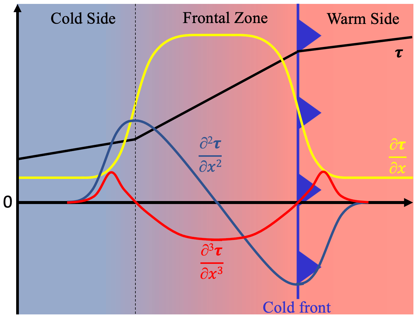
https://gmd.copernicus.org/articles/16/4427/2023/gmd-16-4427-2023-f01

Figure 1Illustration of the thermal-gradient-based detection method, using a simplified straight front and following Hewson (1998) and Kern et al. (2019). The goal is to determine the warm-air boundary of the frontal zone (i.e. the region of increased thermal gradient; see the yellow line). This boundary corresponds to the third derivative (red line) of a thermal variable τ (black line) being zero, under the condition that the second derivative of τ (blue line) is negative. The cold-front typing shown assumes air masses are moving from left to right across the figure.

Download

2.2 Filtering

To obtain meaningful frontal surfaces (or frontal lines in the 2-D case), the feature candidates need to be filtered. Hewson (1998), following Renard and Clarke (1965), suggested to filter according to the thermal front parameter TFP, as well as to a frontal strength value estimated by the local thermal gradient at the frontal feature. The latter was improved by Kern et al. (2019) to estimate frontal strength by computing an average thermal gradient along “normal curves” traced through the frontal zone (basically streamlines computed on the gradient vector field). Here, we generalize these two filters to more generic types of filter mechanisms that can be interactively modified and combined during the analysis to investigate different aspects of the data.

a.
Masking. The feature candidates are filtered according to an arbitrary 3-D scalar field that is sampled (i.e. interpolated) at all feature locations (e.g. if isosurfaces are extracted using marching cubes, at all vertices of the isosurface). User-defined thresholds of the scalar field are used to keep or discard features.
b.
Frontal zone traversal. The frontal zone is traversed along “normal curves” started at feature candidate vertices and computed on the thermal gradient field (Kern et al., 2019); an arbitrary 3-D scalar field is sampled along the normal curves, and filtering thresholds are based on the obtained samples.

The generalization allows us, in addition to filtering with respect to TFP and frontal strength, to add filters that facilitate focus on the contribution of further quantities, including, for example, humidity and elevation. In this way, we can eliminate, for example, pure “humidity fronts” by tracing the changes in (dry) potential temperature (θ) along the normal curves. TFP and frontal strength, however, remain as the core filters.

2.2.1 TFP masking

TFP is a masking filter. Note that computing isosurfaces of L_τ=0 results in front feature candidates at both the cold and the warm sides of the frontal zone. Since we are interested in the warm side only (see Renard and Clarke, 1965), cold side feature candidates need to be discarded. We follow the approach of Hewson (1998) and use the TFP filter, first introduced by Renard and Clarke (1965). The TFP filter is defined as follows:

\begin{matrix} (2) & {TFP}_{τ} \equiv - \nabla_{h} |\nabla_{h} τ| \cdot \frac{\nabla_{h} τ}{|\nabla_{h} τ|} > K_{1}, \end{matrix}

where K₁ is a used-defined threshold. This equation can also be interpreted as the “negative curvature” of the thermal front parameter field (Kern et al., 2019), being positive at the warm side of the frontal zone and negative at the cold side. To obtain only frontal feature candidates at the warm side of the frontal zone, K₁ must be at least zero. Hewson (1998) suggested a slightly positive value for K₁ to eliminate spurious frontal pieces.

2.2.2 Frontal strength

Filters based on normal curves are evaluated for the remaining warm-air-side frontal candidates. We follow Kern et al. (2019) and estimate the frontal strength of the filter variable as “the average thermal gradient along a curved path through the frontal zone from the warm to the cold-air side”. The frontal strength filter S_τ is defined as follows:

\begin{matrix} (3) & S_{τ | frontal zone} \equiv \int_{NC} |\nabla_{h} τ| d s > K_{2} . \end{matrix}

The integration through the frontal zone starts at the warm side of the frontal zone and stops once a “normal curve” reaches the cold side of the frontal zone (where L_τ again is zero). The threshold K₂ is used to eliminate weak fronts below a user-defined frontal strength.

2.2.3 Fuzzy filtering

The usage of distinct threshold values for K₁ and K₂ results in “hard” boundaries of the generated features. Such visualization can be misleading since a viewer can interpret distinct feature boundaries into the depiction (including, for example, “holes” in the front surfaces where, for example, frontal strength is just below the chosen threshold). For fronts, however, this is not the case, as thermal gradients are gradually decreasing in space. Kern et al. (2019) suggested a “soft” (or “fuzzy”) filtering by providing two thresholds for each filter, between which opacity is faded from zero (completely transparent) to one (completely opaque). The feature candidates are subsequently rendered using the obtained opacity, resulting in “fuzzy” edges that visually indicate, , for example, a decreasing thermal gradient. The approach can also facilitate a visual distinction between weak fronts and strong fronts. When multiple filters are used in our implementation, every filter has individual threshold interval settings, and opacity information is accumulated accordingly.

2.3 Supported data and methodological details

The presented algorithm supports gridded data on horizontally regular and rotated latitude–longitude grids. In the vertical, the implementation can handle both pressure levels and model levels. For this study, we use data from the operational ECMWF high-resolution (HRES) forecast with 137 vertical model levels, horizontally interpolated to a regular grid with a grid-point spacing of 0.15^∘ in both latitude and longitude; data from the global reanalysis ERA5 (Hersbach et al., 2020) (also 137 vertical model levels, interpolated to a horizontal grid spacing of 0.25^∘); and data from the COSMO model (Baldauf et al., 2011; Doms and Baldauf, 2018), available on a rotated latitude–longitude grid with 60 vertical model levels and a horizontal grid-point spacing of 0.02^∘ in both dimensions. The algorithm has been integrated into the interactive visualization framework Met.3D (Rautenhaus et al., 2015a) and is being made available as open-source.

In the following, we describe methodological details we deem important for understanding our approach. Figure 2 illustrates the main steps of the front detection process. For simplicity, the process is described for 2-D frontal lines (letters correspond to panels in Fig. 2):

a.
choice of a thermal input field τ (e.g. wet-bulb potential temperature; Fig. 2a)
b.
smoothing of τ (and further input fields used for filtering) to a user-defined length scale (Fig. 2b)
c.
computation of the magnitude of horizontal gradients |∇_hτ| (Fig. 2c)
d.
computation of the horizontal gradient of the magnitude of horizontal gradients ∇_h|∇_hτ| (Fig. 2d)
e.
evaluation of the front location equation Eq. (1) and computation of the zero isolines to obtain feature candidates (Fig. 2e)
f.
computation and application of the TFP masking filter (Fig. 2f)
g.
application of frontal strength and further “normal curve” filters (Fig. 2g)
h.
obtain final frontal structures (Fig. 2h).

In the 2-D example in Fig. 2, the 850 hPa pressure level is used. One important design decision for the 3-D variant of the algorithm is the choice of the vertical coordinate, as the numerical computations need to be implemented accordingly. For this study, we consistently use pressure as the vertical coordinate, i.e. all horizontal computations are evaluated on levels of constant pressure. This is also consistent with Met.3D's use of pressure as the vertical coordinate.

2.3.1 Smoothing

NWP data, especially at kilometre-scale resolution, include convective and thermal processes that are much smaller in scale than atmospheric fronts (Keyser and Shapiro, 1986). To obtain frontal features that meaningfully represent a scale of interest (e.g. synoptic-scale fronts), it is advisable to smooth small-scale thermal fluctuations in the thermal input field. Previous studies have used simple smoothing filters like a weighted moving average of neighbouring grid points (e.g. Jenkner et al., 2009), well-known from image processing (Davies, 2017). Kern et al. (2019) point out that for data on a regular latitude–longitude grid, however, geometric distance between grid points varies with latitude, requiring the usage of a smoothing filter that considers all grid points based on a specified geometric smoothing distance. They propose the usage of a 2-D Gaussian smoothing kernel.

In our implementation, the smoothing distance is a user-defined method parameter that can be interactively changed in the analysis process. A disadvantage of a Gaussian smoothing filter, however, is its computational complexity that increases quadratically with smoothing distance – an important aspect for interactive use. We hence also provide an approximative smoothing method, the “fast almost-Gaussian filtering” presented by Kovesi (2010). The method uses a specified number of averaging passes. More averaging passes increase the accuracy of the approximative algorithm compared to Gaussian smoothing but at the cost of increasing computation time. Another important aspect to consider is that with an increased number of averaging passes the effect of “smoothing over the data field edges” propagates further into the data field centre (Kovesi, 2010). In our implementation, the smoothing computation complexity depends linearly on the averaging passes and the smoothing distance. We find that three averaging passes are a reasonable tradeoff between accuracy, computation time, and keeping the edged effect small. For illustration, we measured the performance of both smoothing algorithms on six cores of an AMD EPYC 7542 32-core processor at 2.9 GHz. In this set-up, it takes about 29.5 s to apply a horizontal Gaussian smoothing with a smoothing distance of 100 km to a 3-D data field of 1800×1800 horizontal grid points with a horizontal grid spacing of 0.02^∘ and 31 vertical level. For the same data field, the approximative algorithm requires 3.9 s. Both algorithms are optimized for OpenMP (OpenMP Architecture Review Board, 2015) and run in parallel.

2.3.2 Numerical implementation

For the computation of horizontal gradients, we use first-order finite central differences and at boundaries first-order finite right and left differences. As described above, we use pressure as the vertical coordinate and hence need to adapt the computations for data available on hybrid sigma pressure model levels or geometric altitude model levels. This leads to an additional coordinate transformation term (see Etling, 2008, pp. 129–131) in the derivatives. The horizontal gradient in pressure coordinates |_p of the thermal variable τ is obtained from the partial derivative in the longitudinal direction on the original coordinate system |_σ and an additional transformation term. The gradient component in the longitudinal direction hence becomes

\begin{matrix} (4) & {\frac{\partial τ}{\partial long}|}_{p} = {\frac{\partial τ}{\partial long}|}_{σ} + \frac{\partial τ}{\partial p}| \cdot {\frac{\partial p}{\partial long}|}_{σ} \end{matrix}

and the latitudinal component

\begin{matrix} (5) & {\frac{\partial τ}{\partial lat}|}_{p} = {\frac{\partial τ}{\partial lat}|}_{σ} + \frac{\partial τ}{\partial p}| \cdot {\frac{\partial p}{\partial lat}|}_{σ} . \end{matrix}

Care needs to be taken for the numerical implementation of Eqs. (1)–(5). For numerical stability reasons, Hewson (1998) computed $\hat{s}$ as a “five-point-mean axis” – an average orientation axis derived from the gradient at the corresponding grid point and at the four surrounding grid points (for details see Hewson, 1998). We encountered challenges with this approach:

a.
The studies by Hewson (1998) and Kern et al. (2019) used gridded data with a regular horizontal grid-point spacing on the order of 50 km (0.5^∘) to 100 km (1^∘). At the time of writing, current (e.g. limited-area) NWP models use finer grid spacings; e.g. the regional forecast model of the German Weather Service (DWD) runs with a horizontal grid spacing of 0.02^∘. At such resolutions and depending on the smoothing distance of previously applied smoothing, the differences between data values at neighbouring grid cells tend to be very small – in such cases, no numerically stable orientation of the five-point-mean axis can be obtained.
b.
Analogous to the above reasons for the use of a distance-based Gaussian smoothing filter, the dependence of geometric distance between neighbouring grid points on latitude leads to inconsistent calculations of the five-point-mean axis.
c.
The distance between neighbouring grid cells depends on the grid-point spacing of the specific dataset used. To compare fronts in different model simulations with a different grid-point spacing it is inconvenient to use a grid-point-based approach because the distance of the neighbouring grid cell changes with changing model resolutions.

Instead of taking the neighbouring grid points to calculate the five-point-mean axis, we propose using interpolated values at a specified distance to the considered central grid point. This improves numerical stability, makes the computation independent of geographic location, and facilitates objective comparison of frontal features obtained from NWP datasets with different grid-point spacings. From our experiments, we find that using a distance for the five-point-mean axis computation of half of the smoothing distance works well.

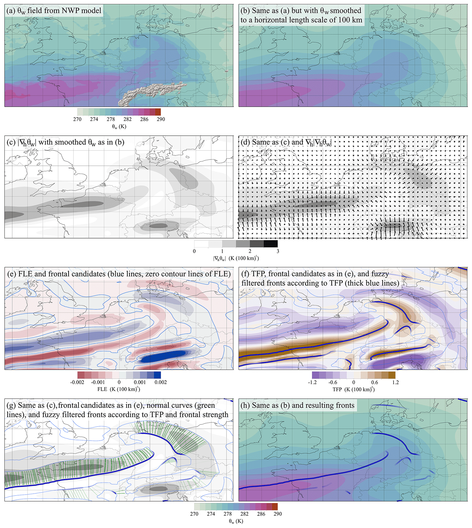
https://gmd.copernicus.org/articles/16/4427/2023/gmd-16-4427-2023-f02

Figure 2Step-by-step illustration of the 2-D front detection method. In the example, objective fronts are based on the 850 hPa wet-bulb potential temperature field (θ_w) from the ECMWF HRES forecast (horizontally regular grid-point spacing of 0.15^∘ in both longitude and latitudes) initialized on 18 January 2018 at 00:00 UTC and valid on 18 January 2018 at 12:00 UTC. Fronts are “fuzzy filtered” using a fade-out range for TFP of 0.2–0.4 K (100 km)⁻² and for frontal strength of 0.6–1 K (100 km)⁻¹. See Sect. 2.3 for a description of panels (a)–(h).

3 Thermal quantity, smoothing length scale, and filter parameters

To successfully apply front detection for case studies, three important aspects need to be considered: which thermal quantity should be used for detection, which smoothing distance should be applied to the data, and how do filter thresholds need to be adjusted (also with respect to the smoothing distance)?

3.1 Choice of thermal quantity

We first discuss the role of the chosen thermal quantity. Three candidates have frequently been used in the literature: (dry) potential temperature (θ), wet-bulb potential temperature (θ_w), and equivalent potential temperature (θ_e). There is an ongoing discussion in the scientific community regarding which thermal quantity is best suited to detect fronts (e.g. Sanders and Doswell, 1995; Hewson, 1998; Berry et al., 2011; Schemm et al., 2018; Thomas and Schultz, 2019a, b). The following provides a brief overview of the potential thermal quantities and their advantages and disadvantages.

The dry potential temperature θ reflects the original, purely temperature-dominated definition of fronts and is most convenient from a rigorous dynamical point of view (Hewson, 1998). However, it is not conserved in moist processes, which often occur along fronts (Browning and Roberts, 1996). Alternative thermal quantities are θ_w or θ_e,which are both conserved in the reversible diabatic processes of evaporation and condensation (Thomas and Schultz, 2019b). Since both quantities have a one-to-one relationship (each θ_w value matches a unique θ_e value and vice versa; Bindon, 1940), they share the same advantages and disadvantages for front detection (Thomas and Schultz, 2019b). In the following, we consider only θ_w; the arguments are similar for θ_e (to detect similar structures, however, the filter thresholds need to be adjusted due to the nonlinear relationship between θ_w and θ_e). The inclusion of humidity can help to better diagnose weak temperature gradients because humidity and temperature gradients are usually correlated, resulting in stronger θ_w gradients compared to θ gradients (Jenkner et al., 2009). However, if humidity and temperature are not correlated, gradients of θ_w could be weaker than gradients of θ. This may result in θ_w fronts being weaker than θ fronts, up to not being detected at all. Furthermore, in regions with humidity gradients but without temperature gradients, purely humidity-dominated fronts can be detected. Therefore, Thomas and Schultz (2019b) recommended examining the temperature and moisture fields separately when analysing frontal structures. On the other hand, Berry et al. (2011) found that in their study θ_w provided the closest match to manually prepared front analysis. In our experience, θ_w is best suited to detect continuous fronts and closely matches the frontal analysis provided by the UK Met Office (Fig. 13). Note that some of the previously mentioned disadvantages of θ_w can be eliminated in our front algorithm. To facilitate the distinction between humidity- and temperature-dominated fronts, the implementation allows the mapping of different quantities on frontal surfaces, as well as the filtering of fronts according to multiple variables. Mapping the total change in θ or specific humidity within the frontal zone could help to distinguish between humidity- and temperature-dominated fronts. If desired, fronts can be filtered according to θ or humidity gradients within the frontal zone, which can help to eliminate purely temperature- or humidity-dominated fronts (Hewson and Titley, 2010).

3.2 Recommendations for filter thresholds and sensitivity of fronts to different smoothing length scales

The number of detected frontal features depends on filter thresholds and the smoothing length scale applied to the input fields. Depending on the scale of interest for the analysis, the horizontal smoothing length scale is chosen. The question arises of which filter thresholds for TFP and frontal strength filters should be recommended and how these values depend on the smoothing length scale. In this section, we explore these method parameters and provide recommendations. We first investigate how smoothing length scale affects the magnitude and distribution of TFP values, and then we consider the magnitude and distribution of frontal strength |∇_hθ_w|. We present distributions of TFP and frontal strength obtained from 24 consecutive time steps of hourly ECMWF HRES forecast data on 18 January 2018 (initialized at 00:00 UTC) in a geographic region encompassing 30^∘ N–70^∘ N in latitude and 60^∘ W–30^∘ E in longitude (slightly larger than the region shown in Fig. 2). The presented distributions provide guidance on the choice of suitable values for different smoothing length scales.

3.2.1 Dependence of filter thresholds K₁ and K₂ on smoothing length scale

Figure 3 shows the relative frequency of TFP values in the analysed area and for three different horizontal smoothing length scales of 100, 50, and 30 km. Large horizontal smoothing length scales result, in general, in lower TFP values and vice versa. With large smoothing applied, strong horizontal gradients are weakened, resulting in smaller horizontal gradients. The magnitude of the horizontal gradients is inversely proportional to the length scale of the horizontal smoothing, and the filter thresholds need to be adjusted accordingly. Table 1 provides our recommendations for fuzzy TFP filter thresholds for the discussed smoothing scales.

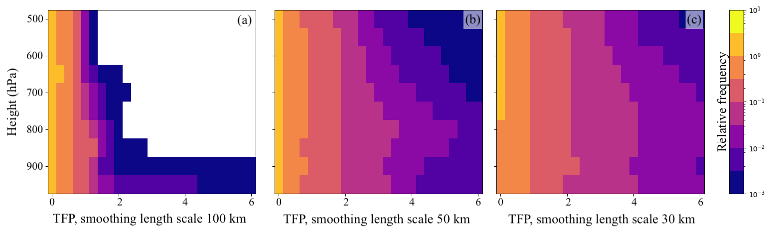
https://gmd.copernicus.org/articles/16/4427/2023/gmd-16-4427-2023-f03

Figure 3Distribution (relative frequencies) of thermal front parameter (TFP) values computed from hourly ECMWF HRES forecast data (horizontal grid-point spacing of 0.15^∘) from 18 January 2018, in the region 30^∘ N–70^∘ N, 60^∘ W–30^∘ E and between 950–500 hPa for different smoothing length scales: (a) 100 km, (b) 50 km, and (c) 30 km.

Download

Figure 4 shows the relative frequency of |∇_hθ_w| for the same smoothing length scales as above, although this time only considering values at grid points within the frontal zone (i.e. where L_τ (Eq. 1) > 0). The same effect encountered for TFP can be observed, and the horizontal smoothing length scale alters the relative frequency of |∇_hθ_w| as well. In general, |∇_hθ_w| decreases with increasing horizontal smoothing length scale. As for TFP, it is necessary to adapt frontal strength filter thresholds to the chosen horizontal smoothing length scale. Table 1 provides guidance.

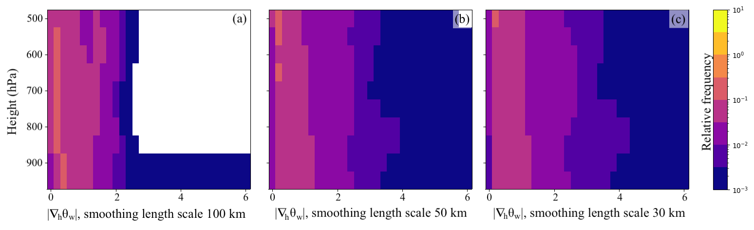
https://gmd.copernicus.org/articles/16/4427/2023/gmd-16-4427-2023-f04

Figure 4Distribution (relative frequencies) of |∇_hθ_w| within frontal zones between 950–500 hPa (same data, time, and region as in Fig. 3) for different smoothing length scales: (a) 100 km, (b) 50 km, and (c) 30 km.

Download

3.2.2 Example: impact of filtering and smoothing on detected frontal features

As mentioned above, NWP data at kilometre-scale resolution includes convective and thermal processes that are much smaller in scale than atmospheric fronts (Keyser and Shapiro, 1986). If the focus of an analysis is on large-scale frontal features, e.g. for large-scale weather analysis, the thermal variable can be smoothed with a distance between 50 and 100 km. If smaller-scale frontal surface phenomena, e.g. surface precipitation, are of interest, the smoothing distance can be reduced to a few kilometres. However, it should not be less than the grid spacing of the thermal input variable. In the following, we demonstrate how different smoothing length scales and filter thresholds impact the resulting frontal features. In particular, we show how different frontal strength filters can help distinguish between different front types (temperature- and humidity-dominated fronts).

Figure 5a extends the 2-D visualization of Fig. 2h to 3-D, depicting the full 3-D structure of the frontal surfaces. We would also like to point the reader to the Video supplement (Beckert et al., 2022c). We consider the interactive use of the presented method as a key aspect of 3-D analysis, and the video provides an impression of the additional benefit gained through interaction.

The 3-D depiction in Fig. 5a reveals further frontal structures such as the large-scale frontal surface in the north (marked with a black arrow in Fig. 5b), which is located above the 850 hPa level and could easily be missed in a 2-D analysis. Not missing such potentially interesting structures is a key benefit of 3-D front detection compared to 2-D detection. Figure 5c–d show temperature-dominated fronts, obtained by applying an additional normal curve filter of θ with a fuzzy threshold interval of 0.6–1.0 K (100 km)⁻¹, the same value range used for θ_w (see Fig. 2). This filter discards all humidity-dominated fronts. Note that the interactive adjustment of the filter is also illustrated in the Video supplement (Beckert et al., 2022c). The blue circle in Fig. 5c highlights an area of the cold front – note how upper-level parts (lighter green, towards the south) are discarded when the humidity contribution is filtered. The vertical cross-section in Fig. 5d shows θ and |∇_hθ|, with the black arrow pointing at the area of the filtered-out upper-level humidity-dominated front. The vertical cross-section also shows no temperature gradients, consistent with the interpretation that this is a humidity-dominated front. In Fig. 5e–f a normal curve filter using a specific humidity filter is applied instead, shifting focus to humidity contribution and discarding temperature-dominated gradients in θ_w. In other words, temperature-dominated fronts are filtered out. The black circle in Fig. 5e marks an area where a large-scale upper-level front is almost entirely discarded.

Finally, Fig. 5g shows the impact of decreasing the smoothing length scale from 100 to 30 km. This reveals frontal features on a different length scale. However, without adjusting the filter thresholds, the resulting fronts become cluttered. Figure 5h shows the same fronts as in Fig. 5g but with adapted filter thresholds to compensate for the reduced horizontal smoothing length scale. Due to reduced smoothing, the smoothness of the frontal surfaces is reduced. Especially at the cold front, fluctuations in θ_w cause less-continuous fronts (red circle). In addition, the reduced smoothing reveals other frontal features on smaller scales; for example, the wrap-up of the occluded front around the cyclone centre is more pronounced (orange arrow). Our recommendations for appropriate filter parameter intervals for different smoothing scales are summarized in Table 1 and are used throughout the paper, except where noted.

Table 1Fuzzy frontal filter threshold recommendations for different smoothing length scales.

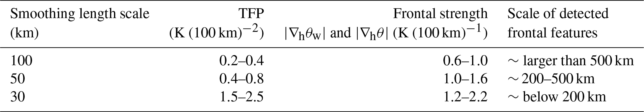
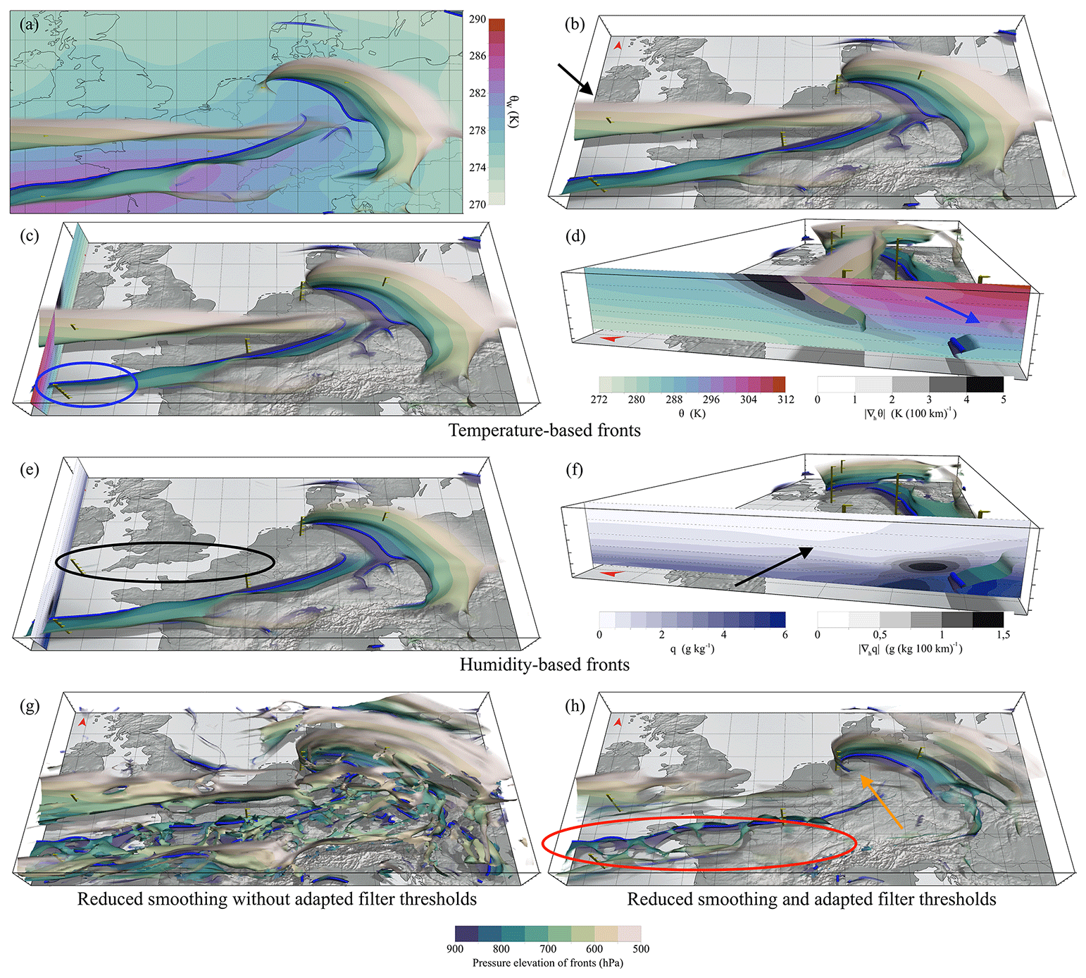
Download Print Version | Download XLSX

https://gmd.copernicus.org/articles/16/4427/2023/gmd-16-4427-2023-f05

Figure 5From 2-D to 3-D objective fronts. Same data as in Fig. 2 (18 January 2018, 12:00 UTC) but showing the full 3-D structure of frontal surfaces in the lower and middle atmosphere. All circles and arrows denote features discussed in text. (a) 850 hPa frontal lines from Fig. 2h with 3-D frontal surfaces between surface and 500 hPa, viewed from the top. (b) Same as (a) but from a tilted viewpoint looking north. (c) Same as (b) but with additional fuzzy normal curve filter of θ between 0.6–1 K (100 km)⁻¹. (d) Same as (c) but viewed from west. Cross section shows θ and |∇_hθ|. (e) Same as (b) but with additional fuzzy normal curve filter of specific humidity between 0.1–0.2 g (kg 100 km)⁻¹. (f) Same as (e) but viewed from west. Cross section shows q and |∇_hq|. (g) Input field smoothed to a horizontal length scale of 30 km with same filtering applied as in (a). (h) Same as (g) but with adapted filter settings for TFP between 1.5–2.5 K (100 km)⁻² and frontal strength between 1.2–2.2 K (100 km)⁻¹.

4 Case studies

We illustrate how meteorological analysis can be performed using 2-D and 3-D front detection by investigating two case studies of extra-tropical cyclones. The first case, Cyclone Vladiana, occurred in the North Atlantic in September 2016. Section 4.2 describes the synoptic situation and the data used for our analysis. For Vladiana, we examine the conceptual model of WCB ascent in the vicinity of fronts (Sect. 4.2.1) and show how frontal surfaces from convection-permitting NWP simulations compare to those found in simulations in which convection is parameterized (Sect. 4.2.2). The second case, Cyclone Friederike, took place in western Europe in January 2018 (introduced in Sect. 4.3). For Friederike, we examine the development stages of a Shapiro–Keyser cyclone in 3-D (Sect. 4.3.1). Additionally, we compare our results to fronts analysed by the UK Met Office to discuss secondary fronts as often shown in surface analysis charts of the UK Met Office (Sect. 4.3.2). Before introducing our case studies, we briefly revisit the underlying meteorological theory in Sect. 4.1.

4.1 Meteorological theory

The frontal structure of extra-tropical cyclones is a key feature for the analysis of their development. Typically, extra-tropical cyclones are classified as either classical Norwegian cyclones (Bjerknes, 1919) or (the later proposed) Shapiro–Keyser cyclones (Shapiro and Keyser, 1990). The development of both cyclone types is classified into four characteristic stages. A cyclone first develops along a frontal wave as a small disturbance near the surface (stage I in both models). Meanwhile, this disturbance strengthens and extends to higher elevations, and the cyclone starts to rotate cyclonically and forms a warm sector (stage II). In stage II the warm sector has its maximum size and maximum energy conversion. For Norwegian cyclones the displacement speed of the cold front is faster than of the warm front, and the warm sector diminishes (stage III). The fronts occlude forcing the air to rise before the cyclone finally dissipates (stage IV). In contrast, a Shapiro–Keyser cyclone develops a frontal fracture in stage II separating the cold front from the warm front. While the cold front is usually weaker than in Norwegian cyclones (Schultz et al., 1998), the warm front is north of the cyclone centre and starts wrapping around it bending backwards and hence is also called bent-back front (stage III). This stage is also called “T-bone structure”. With the warm front wrapping around the cyclone centre, a warm seclusion occurs (stage IV) before the cyclone decays. More recent literature proposes an extension of the four stages by three additional stages: the diminutive frontal wave stage and frontal wave stage which occur before stage I and a decay stage after stage IV (Hewson and Titley, 2010). However, in this publication we focus on the initially proposed four stages of the Shapiro–Keyser cyclone model.

Both cyclone models can be accompanied by coherent circulation features called conveyor belts. The cold conveyor belt occurs ahead of the warm and occlusion front, usually remaining below 850 hPa. It is often associated with high wind speeds in later stages, typically south-west of the cyclone centre. The WCB (see Eckhardt et al., 2004; Madonna et al., 2014) occurs ahead of the cold front near the surface in early stages and is also associated with high wind speeds. It typically ascends at least 600 hPa in the warm sector and over the warm front and often splits into anticyclonically and cyclonically turning branches (Martínez-Alvarado et al., 2014).

4.2 Vladiana

The extra-tropical Cyclone Vladiana occurred during the North Atlantic Waveguide and Downstream Impact Experiment (NAWDEX; Schäfler et al., 2018). Vladiana formed on 22 September 2016 near Newfoundland, and the frontal wave intensified while moving eastwards across the North Atlantic. As the cyclone continued to move north-eastward, it strengthened until it reached its pressure minimum of 975 hPa at 18:00 UTC on 23 September. On 24 September the cyclone reached Iceland and became stationary. Figure 6 shows a horizontal section of θ_w with detected 2-D fronts at 850 hPa, as well as 3-D fronts on 23 September 2016 at 06:00 UTC. The frontal analysis of this case study builds upon previous studies of Vladiana and its associated WCB ascent (Kern et al., 2019; Oertel et al., 2019, 2020; Choudhary and Voigt, 2022). Based on the results of Oertel et al. (2019), we evaluate the conceptual model of 3-D fronts and WCB ascent (Sect. 4.2.1) and illustrate differences in the frontal structure of simulations with explicit vs. parameterized deep convection (Sect. 4.2.2). For our analysis we use ECMWF HRES analysis data with parameterized convection, a convection-permitting simulation with the limited-area model COSMO, and UK Met Office surface analysis charts. Initial and lateral boundary conditions of the COSMO simulation were taken from the ECMWF HRES analysis (see Oertel et al., 2019 and 2020, for a detailed description of the simulation set-up). The COSMO simulation includes online trajectories (see Miltenberger et al., 2013) which were used to select strongly ascending trajectories with ascent rates of at least 600 hPa in 48 h, here referred to as WCB trajectories (Oertel et al., 2019, 2020). For the evaluation of the conceptual model of 3-D fronts and WCBs, WCB trajectories that ascend at least 25 hPa in 2 h at 06:00 UTC on 23 September 2016 were selected.

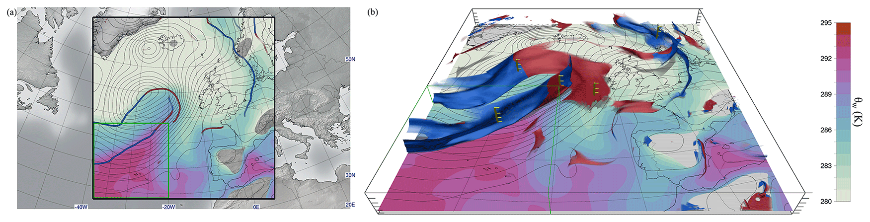
https://gmd.copernicus.org/articles/16/4427/2023/gmd-16-4427-2023-f06

Figure 6Cyclone Vladiana on 23 September 2016 at 06:00 UTC. (a) Detected 2-D warm (red line) and cold (blue line) fronts at 850 hPa, θ_w at 950 hPa (colours, in K), and mean sea level pressure (black contour lines, every 2 hPa) from a COSMO simulation (black frame shows domain boundaries; green frame shows the selected sub-region for studying convection in the vicinity of the cold front; see Sect. 4.2.2). (b) Detected 3-D warm (red) and cold (blue) fronts between 950 hPa and 500 hPa, on top of a horizonal map showing θ_w at 950 hPa and mean sea level pressure (black contour lines, every 2 hPa). Warm- and cold-front classification is computed according to warm- and cold-air advection at the front (following Hewson, 1998).

4.2.1 The 3-D examination of conceptual model: fronts and warm conveyor belt

Conceptual models and simplified illustrations are frequently used to explain the relation and dynamics of fronts and the WCB. Figure 7 shows an example of such an illustration in 2-D, but a more sophisticated 3-D representation can be found, for example, in Martínez-Alvarado et al. (2014, their Fig. 1). However, subsequent studies of these 3-D atmospheric features are usually conducted by means of horizontal or vertical 2-D slices through NWP data, and it is less common to use a 3-D representation of 3-D atmospheric features (Rautenhaus et al., 2018). In this section, we demonstrate the use of 3-D front detection to visualize such conceptual models against NWP data by directly representing these features in 3-D.

Figure 8a–c show the evolution of 3-D fronts from 03:00 to 09:00 UTC on 23 September 2016 of Vladiana, together with a selection of WCB trajectories that ascend at the selected times. During this period the frontal system moves eastwards. At 03:00 UTC the selected WCB trajectories are located in the lower troposphere near the surface in the warm sector and move along the cold front in a north-eastward direction (Fig. 8a). At 06:00 UTC most of the WCB trajectories are in their ascent phase (Fig. 8b), and at 09:00 UTC the majority of the WCB trajectories have risen above 500 hPa (Fig. 8c). The selected trajectories have different pathways for their ascent: some rise directly at or ahead of the cold front, and others rise above the warm front. While trajectories rapidly increase in altitude when lifted spontaneously at the cold front, trajectories at the warm front ascend more slowly and gradually. In Fig. 8d–e the difference between cold-frontal and warm-frontal ascent is emphasized. Figure 8d shows frontal surfaces at 06:00 UTC, together with 48 h WCB trajectories with maximum ascent rates faster than 200 hPa within 2 h. Most of these fast-ascending WCB trajectories ascend at the cold front. In contrast, trajectories at the warm front ascend more slowly, with maximum ascent rates below 200 hPa in 2 h (Fig. 8e). In the upper troposphere, the WCB splits into two outflow branches: a cyclonic branch which turns westward and an anticyclonic branch which turns eastwards. WCB trajectories ascending ahead of the cold front tend to take the anticyclonic outflow, while warm-frontal WCB trajectories tend to take the cyclonic outflow. We hypothesize that trajectories that rapidly ascend at the cold front experience jet wind speeds earlier following the anticyclonically turning jet stream and are thus deflected into the downstream ridge (see Fig. 8f). The 3-D visualization corroborates the conceptual model of how WCB ascent relates to fronts and highlights the presence of smaller-scale convective ascent structures embedded in the WCB discussed in recent studies (see Rasp et al., 2016; Oertel et al., 2019, 2020; Blanchard et al., 2020). The 3-D visualization of rapidly and more slowly ascending high-resolution WCB trajectories further shows their similarity to the so-called “escalator–elevator” concept of WCB-embedded convection which was proposed by Neiman et al. (1993) to distinguish between fast ascent and more gradual frontal upglide. By looking at the 3-D structure of the trajectories, this concept appears suitable for this case study.

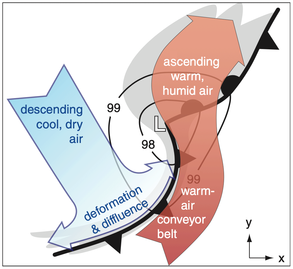
https://gmd.copernicus.org/articles/16/4427/2023/gmd-16-4427-2023-f07

Figure 7Conceptual model of fronts and WCB showing large-scale ascending and descending air in the vicinity of an extra-tropical cyclone (figure adapted from Stull, 2017; © Stull, 2017, CC BY-NC-SA 4.0 license).

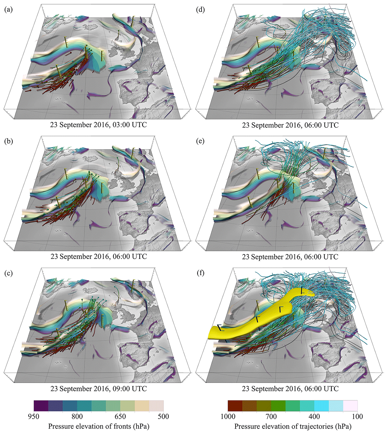
https://gmd.copernicus.org/articles/16/4427/2023/gmd-16-4427-2023-f08

Figure 8(a–c) Temporal evolution of 3-D frontal structures and WCB trajectories of Vladiana on 23 September 2016. (d) Same time as (b) but only fast-ascending WCB trajectories (minimum 200 hPa within 2 h) are displayed for a period of 48 h. (e) Same as (d) but only slow-ascending WCB trajectories (less than 200 hPa within 2 h) are displayed. (f) Same time as (c), jet stream (yellow isosurface of 50 m s⁻¹ wind speed) and WCB trajectories are displayed for a period of 48 h. For the full temporal development of this scene, see the Video supplement (Beckert et al., 2022b).

4.2.2 Cold-front structure in the vicinity of convection

Here we compare fronts of convection-permitting NWP simulations with fronts in simulations where convection is parameterized, using Vladiana as an example. We focus on the southern end of the cold front (green box in Fig. 6) where mid- and small-scale convection occurs in this WCB. Oertel et al. (2019) highlight (embedded) convection with lightning near the trailing edge of the cold front on 23 September 2016 at 06:00 UTC. To detect mid-scale frontal features induced by convection the input field θ_w is smoothed to a horizontal length scale of 50 km and filtered according to TFP, θ_w, and θ (see Table 1). Figure 9 shows detected 2-D fronts at 850 hPa together with fronts of UK Met Office surface charts, at 700 hPa and at 500 hPa. The yellow dot at the southern end of the cold front marks the position of the observed embedded moist convection. The COSMO simulation shows strong ascending motion in this region at all plotted vertical levels (Fig. 9d–f). In contrast, in the ECMWF data (Fig. 9a–c) where convection is parameterized, the vertical velocity field shows no significant local maximum. The detected cold front of both simulations follows the cold front of the UK Met Office surface analysis chart. However, in the vicinity of convection and at 850 hPa the cold front of the COSMO simulation breaks apart, while the cold front detected in ECMWF is a continuous line. At 700 hPa the cold front detected in ECMWF data is weak and broken, while the cold front detected in COSMO data is a continuous line. At 500 hPa the cold front is shifted towards north and is less continuous in the COSMO data compared to ECMWF data.

Figure 10 shows the corresponding 3-D frontal structures. In the area where convective vertical motion differs between the two simulations, a gap can be observed in the frontal surface between 700–600 hPa in the ECMWF data, whereas the frontal surface is present in the COSMO simulation (red circle in Fig. 10a–b). These kinds of gaps in the cold front have been observed in earlier studies (Geerts et al., 2006) and were associated with weaker temperature gradients at this elevation range. The time evolution of the COSMO 3-D front (Fig. A2) suggests that the intensification of the mid-level cold front is a transient feature that occurs at the time of convection, which is associated with strong horizontal convergence (Fig. 10c–d), and disappears as soon as the convection weakens again. In simulations where convection is parameterized, however, the convection scheme may not activate at that time and location. Additionally, the feedback of the convection scheme on the grid-scale variables may differ from their explicit model representation (as shown in this example). We hypothesize that the model representation of convection and/or simulation grid spacing influences the feedback and interaction between convection, frontogenesis, and detailed frontal structures. The investigation of this relation between frontal structure, θ_w gradient, and convective ascent, however, will require more detailed and systematic analyses that are beyond the scope of this study.

https://gmd.copernicus.org/articles/16/4427/2023/gmd-16-4427-2023-f09

Figure 9Convection and frontal structure on 23 September 2016 at 06:00 UTC. Region corresponds to green sub-area in Fig. 6. ECMWF analysis (a, b, c) and COSMO analysis (d, e, f) at (a, d) 850 hPa, (b, e) 700 hPa, and (c, f) 500 hPa. Objective 2-D fronts (blue tubes) are shown along with UK Met Office fronts (red tubes), θ_w (colour), $| \nabla_{h} θ_{w} |$ (grey shades), and upward air velocity (contour lines: orange is upwards, black is zero, and green is downwards; contour line spacing is 0.02 m s⁻¹).

Download

https://gmd.copernicus.org/articles/16/4427/2023/gmd-16-4427-2023-f10

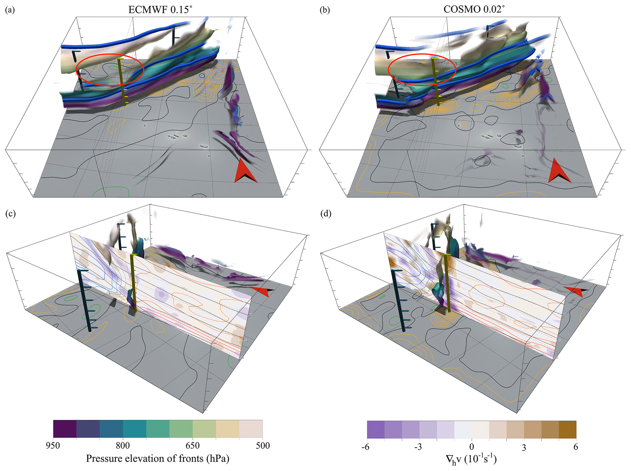
Figure 10The 3-D view of the 2-D frontal structures from Fig. 9. (a) 2-D objective fronts (blue tubes) at 850, 700, and 500 hPa (see Fig. 9) in the context of full 3-D frontal structures, as found in ECMWF data. (b) Same as (a) but for COSMO data. Red circles in (a) and (b) mark the differences in the frontal surfaces. Contour lines on all surface maps represent upward air velocity at 700 hPa (orange is upwards, black is zero, and green is downwards; contour line spacing 0.02 m s⁻¹). (c) ECMWF 3-D fronts and vertical section of wind divergence (colour), θ_w (coloured contour lines, spacing 1 K), and θ (black contour lines, spacing 5 K). (d) Same as (c) but for COSMO data.

Download

4.3 Friederike

The extra-tropical Cyclone Friederike (called David in Great Britain) passed over western Europe from 17 to 18 January 2018. The cyclone had formed east of Florida on 15 January 2018 and then moved northwards along the coast of Newfoundland before it passed the North Atlantic Ocean and first hit Europe at the west coast of Ireland on 17 January 2018. During its passage across the North Atlantic, the cyclone strengthened, and its core pressure dropped to 985 hPa. The cyclone moved from Ireland across northern England and the North Sea, reaching the north of the Netherlands on 18 January 2018 at 09:00 UTC with a core pressure of 976 hPa. From there, the cyclone moved further east and passed northern Germany until it reached the border of Poland on 18 January 2018 at 18:00 UTC and dissipated in the following days. The cyclone caused high wind speeds with gusts up to 203 km h⁻¹ in the Harz Mountains, 144 km h⁻¹ at the North Sea coast of the Netherlands, and 138 km h⁻¹ in lowlands of the Netherlands and central part of Germany (Wandel et al., 2018). Surface analysis charts of the UK Met Office (not shown here) indicate that this was a Shapiro–Keyser cyclone (Shapiro and Keyser, 1990). Our 2-D front algorithm detects some of the characteristic frontal features of the Shapiro–Keyser cyclone, including the frontal wave stage, frontal fracture, and T-bone structure (Fig. 11). This case will allow us for the first time (to our knowledge) to extract and visualize the 3-D frontal structure of a Shapiro–Keyser cyclone directly from NWP data and to evaluate the time evolution in comparison to the conceptual model (Sect. 4.3.1). In Sect. 4.3.2 we analyse the occurrence of secondary warm-frontal structures as often present in surface analysis charts of the UK Met Office.

Here we use the ERA-5 reanalysis and ECMWF HRES forecast data initialized on 18 January 2018 at 00:00 UTC. ERA-5 reanalysis is used to visualize the temporal development of 2-D (Fig. 11) and 3-D (Fig. 12) fronts. For the analysis of secondary frontal structures, fronts extracted from the UK Met Office surface analysis charts supplement the ECMWF HRES forecast.

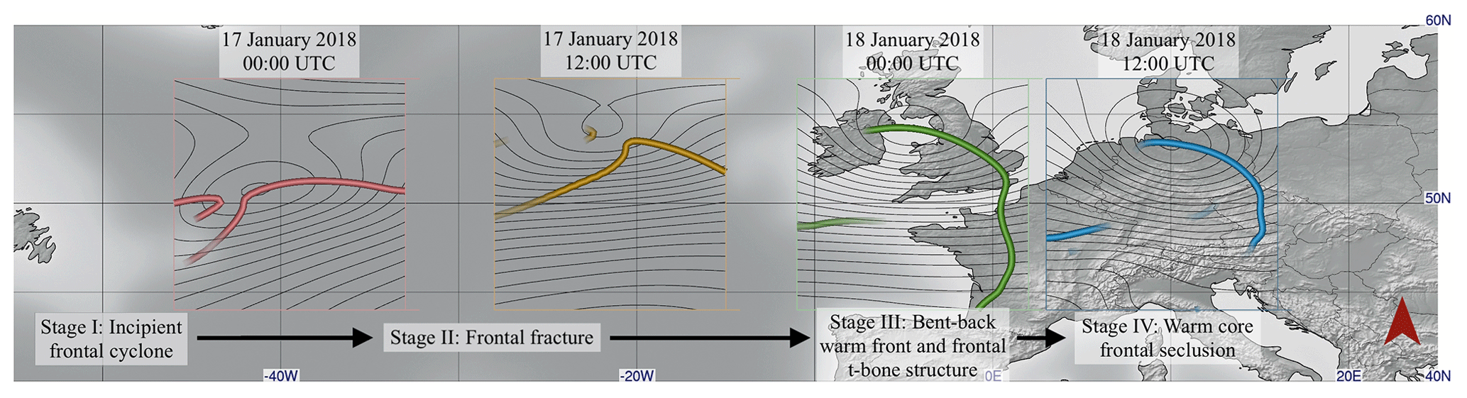
https://gmd.copernicus.org/articles/16/4427/2023/gmd-16-4427-2023-f11

Figure 11Successive time steps of objective 2-D frontal structures showing the temporal development of Friederike (17 and 18 January 2018), as detected in ERA-5 reanalysis data at 750 hPa and surface pressure (black lines). The displayed time steps are approximately assigned to the four ideal development stages of the Shapiro–Keyser cyclone model (Shapiro and Keyser, 1990). We find that not all characteristics of the individual stages can be observed in 2-D. As shown in the following, 3-D front detection is required to observe all characteristics (see Fig. 12).

4.3.1 The 3-D examination of conceptual model: Shapiro–Keyser cyclone

Figure 12 extends the 2-D frontal analysis of Friederike shown in Fig. 11 and shows the temporal development of the 3-D structure. In 3-D, the typical characteristics of a Shapiro–Keyser cyclone (Shapiro and Keyser, 1990) with its distinctive frontal T-bone structure and the four cyclone stages can be observed well. However, at different elevations the four stages, as described in Schultz and Vaughan (2011), occur at different times.

Red and orange front: stage I, incipient frontal cyclone. A perturbation of the frontal structure is already present in the upper atmosphere. This disturbance will later develop into the frontal wave. However, the frontal surface in the lower atmosphere is unperturbed.
Orange, yellow, green front: stage II, frontal fracture. The timing of frontal fracture strongly depends on the vertical level. In the lower troposphere the cold front is separating from the main front. In the upper troposphere, a connection between the cold front and the main part of the frontal surface still exists.
Green and blue front: stage III, bent-back warm front and frontal T-bone structure. At lower levels, the cold front lies almost perpendicular to the warm front, showing the typical Shapiro–Keyser T-bone structure. Interestingly, the upper part of the cold front also bends slightly towards the south, following the lower part of the cold front, but a connection to the warm front remains.
Blue and purple front: stage IV, warm-core frontal seclusion. The warm front wraps up around the warm air near the cyclone centre. The separated lower part of the cold front moves further south, and the upper cold front dissipates.

In this example, uniquely assigning the 3-D frontal structure at specific time steps to the Shapiro and Keyser stages is not possible. As described, frontal evolution does not occur synchronously at all elevations, creating a temporal offset of the stages at different elevations. We could also not find a height level where the 2-D fronts could be uniquely assigned (see Fig. 11). It is important, however, that the 3-D front detection can detect all the characteristic structures of the Shapiro–Keyser model, even though a one-to-one assignment to the stages is not possible. Another example of the 3-D frontal development with typical characteristics of a Shapiro–Keyser cyclone, Cyclone Egon (11–13 January 2017; Eisenstein et al., 2020), is shown in Fig. A1 in the Appendix of this study. Again, the visual analysis shows that frontal evolution does not occur synchronously at all elevations, creating a temporal offset. For example, frontal fracture does not occur at all elevations simultaneously. The time step on 13 January 2017 at 00:00 UTC shows the development of the bent-back warm front in upper levels, whereas the frontal fracture is not yet complete near the surface. These examples suggest a more nuanced view of the Shapiro–Keyser model, where there is a significant 3-D component to the evolution of a cyclone through the different stages of the conceptual model.

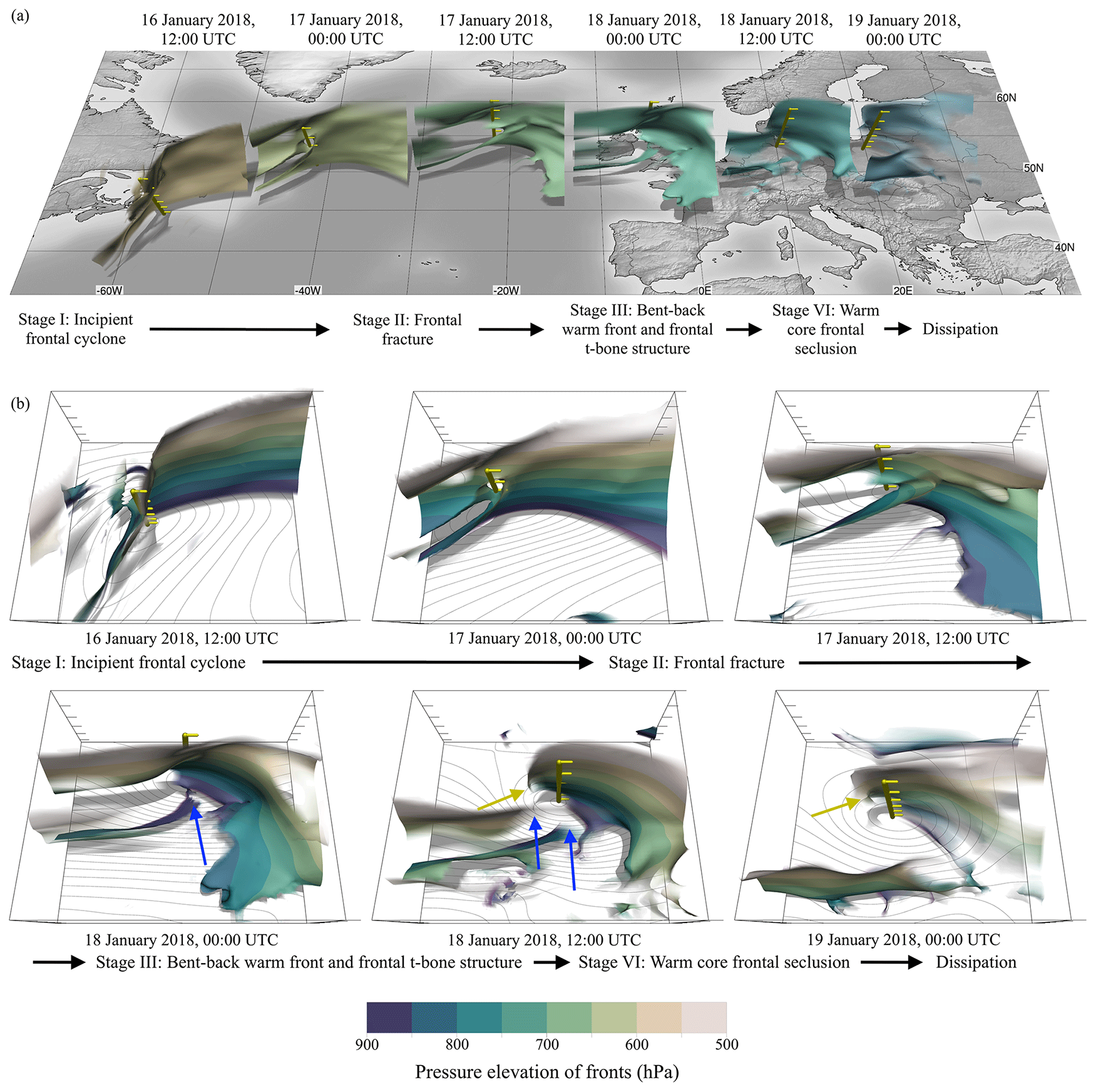
https://gmd.copernicus.org/articles/16/4427/2023/gmd-16-4427-2023-f12

Figure 12Temporal evolution of 3-D frontal structures of Friederike (16 to 19 January 2018), as detected in ERA-5 reanalysis data. (a) Different cyclone stages encountered along the cyclone track. Yellow poles mark centres of surface low, and front colours distinguish time steps. (b) The six stages from (a), approximately centred around the cyclone centres for comparison of frontal structures. Blue arrows mark frontal fracture, yellow arrows mark warm-core frontal seclusion, and contour lines show surface pressure (spacing 2 hPa).

4.3.2 Secondary fronts

Secondary fronts are commonly analysed by the UK Met Office and seen in their surface analysis charts. Beside other variables, the UK Met Office uses the wet-bulb potential temperature as the primary thermal variable for their front detection in surface analysis charts (Neil Armstrong, UK Met Office, personal communication, 2022). In this section, we consider a secondary front which occurs ahead of the warm front of Friederike. We investigate if the front detection algorithm can detect such secondary fronts and how secondary fronts depend on the detection variable. Red tubes in Fig. 13 show the positions of fronts analysed by the UK Met Office for 18 January 2018 at 12:00 UTC. The most eastward front, extending from north-east Italy up to the southern border of Denmark, is a typical secondary warm front as often analysed by the UK Met Office. Figure 13b shows fronts detected in θ_w at 850 hPa (blue tubes). In general, the structure of fronts detected in θ_w agrees well with fronts of the UK Met Office, despite some smaller differences. In particular, the secondary front detected in θ_w is shorter in its horizontal extent, and the wrap-up of the occluded front around the cyclone centre is more pronounced. Figure 13c shows fronts detected in θ at 850 hPa (green tubes). There is no indication for secondary fronts in this analysis, as no strong horizontal gradients of θ are present in this area. Hence, the presence of the secondary front detected by θ_w results from moisture gradients. Furthermore, the structure of the primary fronts is less continuous and deviates more from the UK Met Office analysis. Figure 14 shows the 3-D frontal surfaces of θ_w (Fig. 14a) and θ (Fig. 14b). The 3-D frontal structure illustrates that the secondary front detected in θ_w is a shallow atmospheric feature and is only present in the lower troposphere at around 850 hPa. For this case study we conclude that the lower-atmospheric secondary front is a moisture feature and thus can only be detected in a variable that includes humidity formation. Furthermore, θ_w as the detection variable results in more-continuous fronts compared to θ. We again would like to point the reader to the Video supplement (Beckert et al., 2022c), which illustrates the benefit of interactive exploration and analysis of the detected fronts within Met.3D.

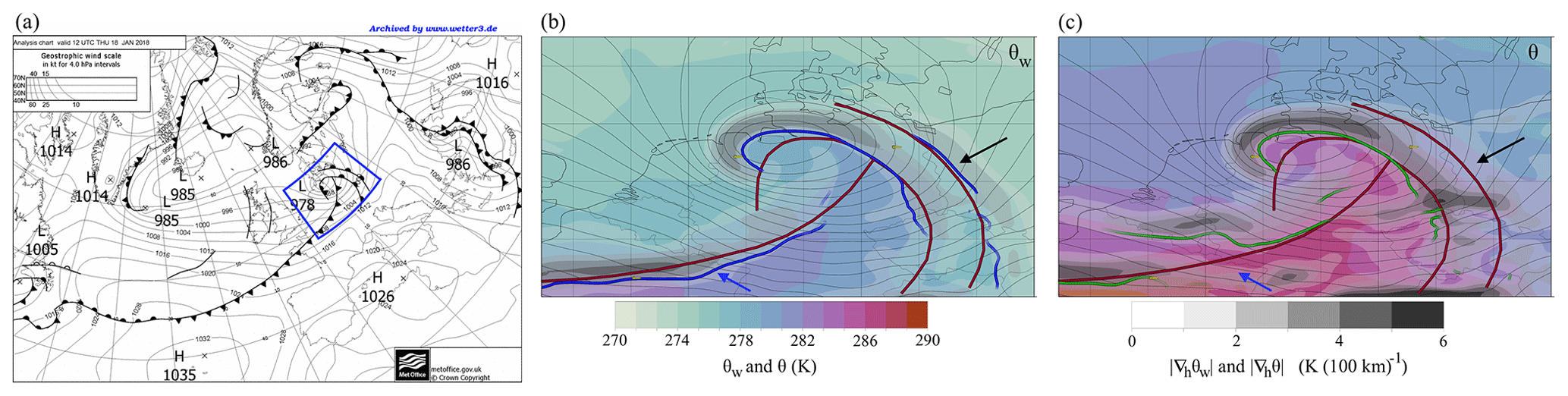
https://gmd.copernicus.org/articles/16/4427/2023/gmd-16-4427-2023-f13

Figure 13Comparison of UK Met Office fronts with objective fronts for case Friederike (18 January 2018, 12:00 UTC). (a) UK Met Office surface analysis chart. Blue box marks analysed area. (b) Objective 850 hPa 2-D fronts (blue lines) as detected from ECMWF HRES θ_w (colour; grey shading shows $| \nabla_{h} θ_{w} |$ ), UK Met Office fronts (red lines), and mean sea level pressure (black contour lines, spacing 2 hPa). (c) Same as (b) but objective 2-D fronts (green lines) based on θ. The secondary front (black arrow) is only detected when using θ_w. When based on θ, the cold front (blue arrow) breaks up and is less continuous compared to the cold front based on θ_w.

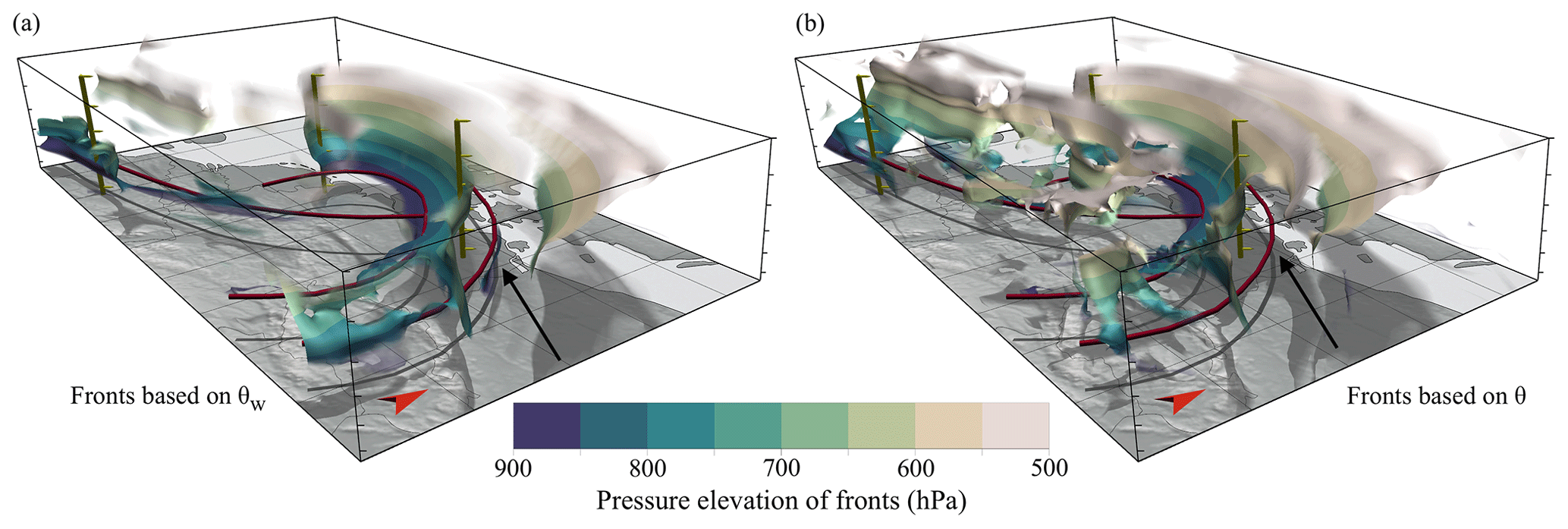
https://gmd.copernicus.org/articles/16/4427/2023/gmd-16-4427-2023-f14

Figure 14The 3-D view of Fig. 13b–c. Red tubes show UK Met Office fronts, and 3-D objective fronts are coloured according to pressure elevation. Objective fronts based on (a) θ_w and (b) θ. The secondary front (black arrow) is a feature of θ_w and only occurs around 850 hPa. Yellow poles are to aid spatial perception. Compare the animated version in the Video supplement (Beckert et al., 2022a).

5 Summary and discussion

This article explores how objective 2-D and 3-D front detection and visualization, integrated into an interactive 3-D visual analysis environment for atmospheric data, can be used to study frontal dynamics within mid-latitude cyclones and thus be beneficial for weather forecasting and research. The presented method builds on approaches previously introduced by Hewson (1998) and Kern et al. (2019) and is applicable to gridded data from state-of-the-art NWP models. It facilitates rapid analysis of 3-D frontal dynamics, including an objective comparison of detected frontal structures between datasets from different numerical models or ensemble members, also at different model resolutions. We addressed the objectives of (a) identifying appropriate detection parameters including data smoothing and filtering thresholds to ensure objective comparability and (b) evaluating the benefit of 3-D IVA of frontal surfaces through case study investigations, including interpretations based on conceptual models, and comparison of frontal structures between different numerical models and with manually produced surface analysis charts.

We find that the integration of 3-D front detection with 3-D IVA (in our case in the open-source meteorological visual analysis framework Met.3D) facilitates rapid analysis of complex weather situations, in part because the detected fronts can be visualized jointly with interactively placed depictions of other meteorological quantities.

The choice of the thermal variable is essential for the presented approach. For the cases presented in this article, we show that θ_w is most suitable, since, in contrast to θ, it considers reversible moist processes in the atmosphere. The resulting fronts are longer and more continuous. A disadvantage of θ_w is that it also detects purely humidity-dominated fronts. Separately filtering frontal feature candidates according to humidity and θ gradients, however, allows us to distinguish humidity-dominated from temperature-dominated fronts. The choice of filter parameters and filter thresholds to obtain meaningful frontal structures is challenging. These settings depend on the thermal input variable's horizontal smoothing length scale, which determines the “spatial scales” of detected frontal features (large-scale smoothing of the thermal input field results in the detection of large-scale frontal features and vice versa). The distribution of gradient magnitudes shows that different smoothing length scales require different filter thresholds to obtain meaningful fronts. Large-scale smoothing requires less restrictive filter thresholds compared to small-scale smoothing. We present recommendations to future users on how to tune filter thresholds according to the previously applied smoothing length scale (Table 1).

The application of the proposed approach to case studies of mid-latitude cyclones provides detailed information about the temporal evolution of 3-D front characteristics. We demonstrate the use of 3-D front detection to visualize dynamic relations of features in the context of fronts in NWP data by directly representing these features in 3-D. In a case study of Cyclone Vladiana (September 2016) we examine the conceptual model of the WCB as represented by NWP data. At the cold front, WCB trajectories ascend fast, experience jet wind speeds early, and follow the anticyclonically turning jet stream. In contrast, WCB trajectories ascending at the warm front show a slower ascent rate and tend to take the cyclonic outflow branch in the upper troposphere. These observations agree well with conceptual models of fronts and WCB as proposed in the literature. Our next example considers the relation between convection and cold-front structure. For Vladiana, the cold front at mid-tropospheric levels is temporarily strengthened in the vicinity of resolved convection; we hypothesize that the model representation of convection and/or simulation grid spacing influences the feedback and interaction between convection, frontogenesis, and detailed frontal structures. In a second case study of Cyclone Friederike (January 2018), we visually analyse the 3-D temporal evolution of fronts in a Shapiro–Keyser cyclone and compare our results to the conceptual model proposed in the literature. We observe that the different Shapiro–Keyser cyclone stages do not occur simultaneously at all elevations. However, all characteristic stages of the conceptual model of the Shapiro–Keyser cyclone could be observed in NWP data. Finally, we compare the objective 3-D frontal structures with 2-D fronts in UK Met Office surface analysis charts and investigate the occurrence of secondary fronts often present in UK Met Office surface analyses. The objective 3-D fronts are consistent with the UK Met Office fronts if θ_w is used for front detection. This is no coincidence as θ_w is the primary thermal variable used for the manual front detection by the UK Met Office. For Friederike, we show that the secondary front corresponds to a humidity-dominated rather than a temperature-dominated front. An in parts similar front detection approach – only two-dimensional but also applicable to kilometre-scale resolution data – was proposed by Jenkner et al. (2009). Because of high sensitivity to local noise in higher derivatives, their approach uses the zero lines of the TFP (second derivative) as frontal candidates, which correspond to the steepest gradient within the frontal zone. However, this does not match the most common definition of a front as the boundary of the frontal zone located on the warm-air side (see Renard and Clarke, 1965). We argue that an advantage of our approach in particular for case studies is that also in kilometre-scale data fronts are detected at this warm-air side, albeit at the cost of potential smoothing artefacts.

Opportunities for future novel methods may be facilitated by recent advances in machine learning (ML). For example, an approach using artificial neural networks to detect 2-D fronts was recently proposed by Niebler et al. (2022). Their approach learns from fronts depicted on analysis charts issued by national weather services and hence mimics the approaches of human forecasters. Will such ML-based approaches be able to detect robust 3-D structures in the future?

As a final remark, the front detection and visualization approach presented here has the potential to be used operationally. Being integrated in Met.3D, other meteorological variables can be analysed in conjunction with the 3-D frontal structures. This facilitates the rapid analysis of complex weather situations, as required in operational settings (see Rautenhaus et al., 2018). Further fields of application include the feature-based analysis of forecast uncertainty represented by ensembles simulations (albeit comparative visualization of features from many ensemble members will be challenging), climatological studies of frontal characteristics derived from the 3-D features, and investigation of the relation of frontal structures to other physically meaningful features in the 3-D atmosphere, including the jet stream – this will be beneficial for studies that contribute to the understanding of complex dynamical processes in the atmosphere.

Appendix A

https://gmd.copernicus.org/articles/16/4427/2023/gmd-16-4427-2023-f15

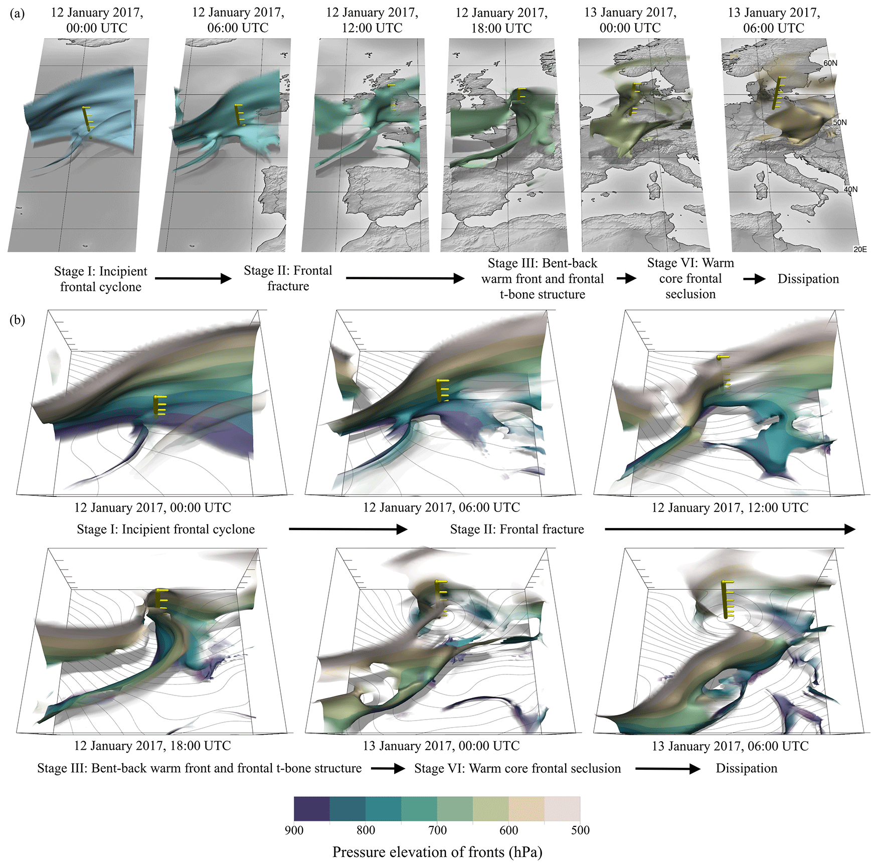
Figure A1Temporal evolution of 3-D frontal structures of Egon (12 to 13 January 2017), as detected in ERA-5 reanalysis data. (a) Different cyclone stages encountered along the cyclone track. Yellow poles mark centres of surface low, and front colours distinguish time steps. (b) The six stages from (a), approximately centred around the cyclone centres for comparison of frontal structures. Contour lines show surface pressure (spacing 2 hPa).

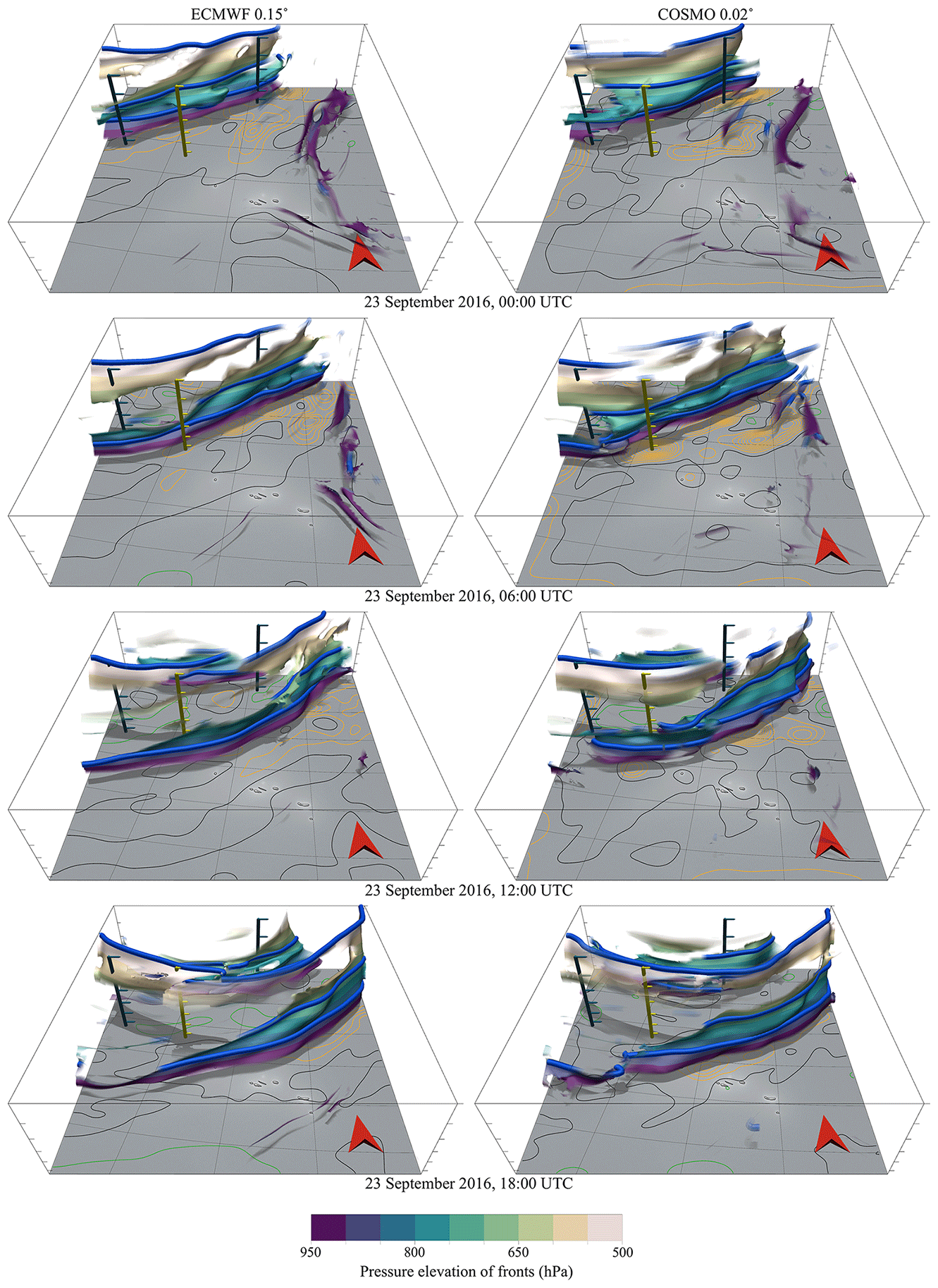
https://gmd.copernicus.org/articles/16/4427/2023/gmd-16-4427-2023-f16

Figure A2Temporal evolution of 3-D frontal structures in Fig. 10, detected from (left) ECMWF analysis and (right) COSMO analysis. Contour lines projected onto the surface show upward air velocity at 700 hPa (orange is upwards, black is zero, and green is downwards; contour line spacing of 0.02 m s⁻¹). The yellow pole marks the centre of the convective updraft at 06:00 UTC, and the red arrow points northward.

Download

Code and data availability

The code of the specific version of the open-source visualization framework Met.3D, including the code for front detection and example configuration files to reproduce figures of this paper, is available at https://doi.org/10.5281/ZENODO.7870254 (Beckert et al., 2023). User and developer documentation is available at https://met3d.wavestoweather.de (Met.3D – Homepage, 2022) and https://collaboration.cen.uni-hamburg.de/display/Met3D/ (Met.3D – Documentation, 2022). The ECMWF ERA5 and ECMWF HRES forecast and analysis datasets used in this study are available at https://doi.org/10.5281/ZENODO.7875629 (Beckert, 2023). Please contact the authors for information about the COSMO dataset.

Video supplement

The following movies illustrate interactive visual data analysis using Met.3D and provide supplementary insights into the 3-D dynamics of frontal structures, jet stream, and WCB trajectories, and they also illustrate the benefit gained from interactive use of 3-D visual analysis:

comparison of objectively detected 3-D fronts in wet-bulb potential temperature and potential temperature of Friederike on 18 January 2018 at 12:00 (https://doi.org/10.5446/57600, Beckert et al., 2022a);
development of 3-D frontal structures, jet stream, and WCB trajectories of Vladiana (https://doi.org/10.5446/57570, Beckert et al., 2022b);
interactive front analysis of storm Friederike using the open-source meteorological 3-D visualization framework “Met.3D” (https://doi.org/10.5446/57944, Beckert et al., 2022c).

Author contributions

AAB designed and implemented the algorithm, performed the analysis, created the visualizations, and wrote the manuscript. LE contributed to the meteorological-related results, especially to the characterization and discussion of the Shapiro–Keyser cyclone. AO contributed to the meteorological-related results, especially to the characterization and discussion of the WCB. TH contributed to the design of the algorithm and secondary front discussion. MR and GC proposed, supervised, and administrated the study. All authors contributed to writing and revising the manuscript.

Competing interests

The contact author has declared that none of the authors has any competing interests.

Disclaimer

Publisher's note: Copernicus Publications remains neutral with regard to jurisdictional claims in published maps and institutional affiliations.

Acknowledgements

This research leading to these results has been done within sub-projects C9 (Andreas A. Beckert, George Craig, Marc Rautenhaus), C5 (Lea Eisenstein), and B8 (Annika Oertel) of the Transregional Collaborative Research Center SFB/TRR165 “Waves to Weather” (https://www.wavestoweather.de/, last access: 16 November 2022) funded by the German Research Foundation (DFG). The authors would like to thank the Institute for Atmospheric and Climate Science at ETH Zürich for providing the high-resolution COSMO dataset of Vladiana. We also very much thank the two anonymous reviewers and the editor.

Financial support

This research has been supported by the Deutsche Forschungsgemeinschaft (project C9, C5, and B5 in the Transregional Collaborative Research Centre SFB/TRR 165 “Waves to Weather”; grant no. 257899354 – TRR 165).

Review statement

This paper was edited by Richard Neale and reviewed by two anonymous referees.

References

Aemisegger, F., Spiegel, J. K., Pfahl, S., Sodemann, H., Eugster, W., and Wernli, H.: Isotope meteorology of cold front passages: A case study combining observations and modeling, Geophys. Res. Lett., 42, 5652–5660, https://doi.org/10.1002/2015GL063988, 2015.

Bader, M. J., Forbes, G. S., Grant, J. R., Lilley, R. B. E., and Waters, A. J.: Images in Weather Forecasting: A Practical Guide for Interpreting Satellite and Radar Imagery, 523 pp., ISBN-13 978-0521451116, 1996.

Bader, R., Sprenger, M., Ban, N., Radisuhli, S., Schar, C., and Ganther, T.: Extraction and Visual Analysis of Potential Vorticity Banners around the Alps, IEEE Trans. Vis. Comput. Graph., 26, 1–1, https://doi.org/10.1109/TVCG.2019.2934310, 2020.

Baldauf, M., Seifert, A., Förstner, J., Majewski, D., Raschendorfer, M., and Reinhardt, T.: Operational convective-scale numerical weather prediction with the COSMO model: Description and sensitivities, Mon. Weather Rev., 139, 3887–3905, https://doi.org/10.1175/MWR-D-10-05013.1, 2011.

Beckert, A.: Datasets associated with the publication: “The three-dimensional structure of fronts in mid-latitude weather systems in numerical weather prediction models”, Zenodo [data set], https://doi.org/10.5281/ZENODO.7875629, 2023.

Beckert, A., Rautenhaus, M., Kern, M., and Met.3D-Contributors: met.3d-1.8.0_3DFronts_v1.0, Zenodo [code], https://doi.org/10.5281/ZENODO.7870254, 2023.

Beckert, A. A., Eisenstein, L., Oertel, A., Hewson, T., Craig, G. C., and Rautenhaus, M.: Comparison of objectively detected 3-D fronts in wet-bulb potential temperature and potential temperature, TIB AV Portal [video], https://doi.org/10.5446/57600, 2022a.

Beckert, A. A., Eisenstein, L., Oertel, A., Hewson, T., Craig, G. C., and Rautenhaus, M.: Development of 3-D frontal structures, jet stream and WCB trajectories of Vladiana, TIB AV Portal [video], https://doi.org/10.5446/57570, 2022b.

Beckert, A. A., Eisenstein, L., Oertel, A., Hewson, T., Craig, G. C., and Rautenhaus, M.: Interactive front analysis of storm Friederike using the open-source meteorological 3-D visualization framework “Met. 3D,” TIB AV Portal [video], https://doi.org/10.5446/57944, 2022c.

Berry, G., Reeder, M. J., and Jakob, C.: A global climatology of atmospheric fronts, Geophys. Res. Lett., 38, 1–5, https://doi.org/10.1029/2010GL046451, 2011.

Bindon, H. H.: Relation between equivalent potential temperature and wet-bulb potential temperature, Mon. Weather Rev., 68, 243–245, https://doi.org/10.1175/1520-0493(1940)068<0243:RBEPTA>2.0.CO;2, 1940.

Bjerknes, J.: On the structure of moving cyclones, Mon. Weather Rev., 95–99, 1919.

Blanchard, N., Pantillon, F., Chaboureau, J.-P., and Delanoë, J.: Organization of convective ascents in a warm conveyor belt, Weather Clim. Dynam., 1, 617–634, https://doi.org/10.5194/wcd-1-617-2020, 2020.

Bösiger, L., Sprenger, M., Boettcher, M., Joos, H., and Günther, T.: Integration-based extraction and visualization of jet stream cores, Geosci. Model Dev., 15, 1079–1096, https://doi.org/10.5194/gmd-15-1079-2022, 2022.

Browning, K. A. and Monk, G. A.: A Simple Model for the Synoptic Analysis of Cold Fronts, Q. J. Roy. Meteor. Soc., 108, 435–452, https://doi.org/10.1002/qj.49710845609, 1982.

Browning, K. A. and Roberts, N. M.: Variation of frontal and precipitation structure along a cold front, Q. J. Roy. Meteor. Soc., 122, 1845–1872, https://doi.org/10.1002/qj.49712253606, 1996.

Choudhary, A. and Voigt, A.: Impact of grid spacing, convective parameterization and cloud microphysics in ICON simulations of a warm conveyor belt, Weather Clim. Dynam., 3, 1199–1214, https://doi.org/10.5194/wcd-3-1199-2022, 2022.

Davies, E. R.: Computer Vision, Principles, Algorithms, Applications, Learning, 5th Edn., Academic Press, 900 pp., ISBN-13 978-0-12-809284-2, 2017.

Doms, G. and Baldauf, M.: A Description of the Nonhydrostatic Regional COSMO-Model. Part I: Dynamics and Numerics, Report COSMO-Model 5.05, Deutscher Wetterdienst, https://doi.org/10.5676/DWD_pub/nwv/cosmo-doc_5.05_I, 2018.

Eckhardt, S., Stohl, A., Wernli, H., James, P., Forster, C., and Spichtinger, N.: A 15-Year Climatology of Warm Conveyor Belts, J. Climate, 17, 218–237, https://doi.org/10.1175/1520-0442(2004)017<0218:AYCOWC>2.0.CO;2, 2004.

Eisenstein, L., Pantillon, F., and Knippertz, P.: Dynamics of sting-jet storm Egon over continental Europe: Impact of surface properties and model resolution, Q. J. Roy. Meteor. Soc., 146, 186–210, https://doi.org/10.1002/qj.3666, 2020.

Etling, D.: Theoretische Meteorologie Eine Einführung, Springer-Verlag Berlin Heidelberg, 376 pp., ISBN 978-3-540-75978-2, 2008.

Fischer, C., Fink, A. H., Schömer, E., van der Linden, R., Maier-Gerber, M., Rautenhaus, M., and Riemer, M.: A novel method for objective identification of 3-D potential vorticity anomalies, Geosci. Model Dev., 15, 4447–4468, https://doi.org/10.5194/gmd-15-4447-2022, 2022.

Front – Glossary of Meteorology: https://glossary.ametsoc.org/wiki/Front, last access: 28 February 2022.

Geerts, B., Damiani, R., and Haimov, S.: Finescale Vertical Structure of a Cold Front as Revealed by an Airborne Doppler Radar, Mon. Weather Rev., 134, 251–271, https://doi.org/10.1175/MWR3056.1, 2006.

Hersbach, H., Bell, B., Berrisford, P., Hirahara, S., Horányi, A., Muñoz-Sabater, J., Nicolas, J., Peubey, C., Radu, R., Schepers, D., Simmons, A., Soci, C., Abdalla, S., Abellan, X., Balsamo, G., Bechtold, P., Biavati, G., Bidlot, J., Bonavita, M., Chiara, G., Dahlgren, P., Dee, D., Diamantakis, M., Dragani, R., Flemming, J., Forbes, R., Fuentes, M., Geer, A., Haimberger, L., Healy, S., Hogan, R. J., Hólm, E., Janisková, M., Keeley, S., Laloyaux, P., Lopez, P., Lupu, C., Radnoti, G., Rosnay, P., Rozum, I., Vamborg, F., Villaume, S., and Thépaut, J.: The ERA5 global reanalysis, Q. J. Roy. Meteor. Soc., 146, 1999–2049, https://doi.org/10.1002/qj.3803, 2020.

Hewson, T. D.: Objective fronts, Meteorol. Appl., 5, 37–65, https://doi.org/10.1017/S1350482798000553, 1998.

Hewson, T. D. and Titley, H. A.: Objective identification, typing and tracking of the complete life-cycles of cyclonic features at high spatial resolution, Meteorol. Appl., 17, 355–381, https://doi.org/10.1002/met.204, 2010.

Huber-Pock, F. and Kress, C.: An operational model of objective frontal analysis based on ECMWF products, Meteorol. Atmos. Phys., 40, 170–180, https://doi.org/10.1007/BF01032457, 1989.

Jenkner, J., Sprenger, M., Schwenk, I., Schwierz, C., Dierer, S., and Leuenberger, D.: Detection and climatology of fronts in a high-resolution model reanalysis over the Alps, Meteorol. Appl., 17, 1–18, https://doi.org/10.1002/met.142, 2009.

Kern, M., Hewson, T. D., Sadlo, F., Westermann, R., and Rautenhaus, M.: Robust Detection and Visualization of Jet-Stream Core Lines in Atmospheric Flow, IEEE Trans. Vis. Comput. Graph., 24, 893–902, https://doi.org/10.1109/TVCG.2017.2743989, 2018.

Kern, M., Hewson, T. D., Schäfler, A., Westermann, R., and Rautenhaus, M.: Interactive 3D Visual Analysis of Atmospheric Fronts, IEEE Trans. Vis. Comput. Graph., 25, 1080–1090, https://doi.org/10.1109/TVCG.2018.2864806, 2019.

Keyser, D. and Shapiro, M. A.: A Review of the Structure and Dynamics of Upper-Level Frontal Zones, Mon. Weather Rev., 114, 452–499, https://doi.org/10.1175/1520-0493(1986)114<0452:AROTSA>2.0.CO;2, 1986.

Kovesi, P.: Fast almost-Gaussian filtering, Proc. – 2010 Digit. Image Comput. Tech. Appl. DICTA 2010, 121–125, https://doi.org/10.1109/DICTA.2010.30, 2010.

Locatelli, J. D., Martin, J. E., and Hobbs, P. V.: A wide cold-frontal rainband and its relationship to frontal topography, Q. J. Roy. Meteor. Soc., 120, 259–275, https://doi.org/10.1002/qj.49712051603, 1994.

Locatelli, J. D., Stoelinga, M. T., and Hobbs, P. V.: Re-examination of the split cold front in the British Isles cyclone of 17 July 1980, Q. J. Roy. Meteor. Soc., 131, 3167–3181, https://doi.org/10.1256/qj.04.157, 2005.

Lorensen, W. E. and Cline, H. E.: Marching cubes: A high resolution 3D surface construction algorithm, in: Proceedings of the 14th annual conference on Computer graphics and interactive techniques – SIGGRAPH '87, 163–169, https://doi.org/10.1145/37401.37422, 1987.

Madonna, E., Wernli, H., Joos, H., and Martius, O.: Warm Conveyor Belts in the ERA-Interim Dataset (1979–2010). Part I: Climatology and Potential Vorticity Evolution, J. Climate, 27, 3–26, https://doi.org/10.1175/JCLI-D-12-00720.1, 2014.

Martínez-Alvarado, O., Baker, L. H., Gray, S. L., Methven, J., and Plant, R. S.: Distinguishing the Cold Conveyor Belt and Sting Jet Airstreams in an Intense Extratropical Cyclone, Mon. Weather Rev., 142, 2571–2595, https://doi.org/10.1175/MWR-D-13-00348.1, 2014.

Met.3D – Code Repository: GitLab [code], https://gitlab.com/wxmetvis/met.3d, last access: 15 November 2022.

Met.3D – Documentation: User Documentation, https://collaboration.cen.uni-hamburg.de/display/Met3D/, last access: 15 November 2022.

Met.3D – Homepage: Interactive 3D visualization of meteorological simulations, https://met3d.wavestoweather.de, last access: 15 November 2022.

Meyer, M., Polkova, I., Modali, K. R., Schaffer, L., Baehr, J., Olbrich, S., and Rautenhaus, M.: Interactive 3-D visual analysis of ERA5 data: improving diagnostic indices for marine cold air outbreaks and polar lows, Weather Clim. Dynam., 2, 867–891, https://doi.org/10.5194/wcd-2-867-2021, 2021.

Miltenberger, A. K., Pfahl, S., and Wernli, H.: An online trajectory module (version 1.0) for the nonhydrostatic numerical weather prediction model COSMO, Geosci. Model Dev., 6, 1989–2004, https://doi.org/10.5194/gmd-6-1989-2013, 2013.

Neiman, P. J., Shapiro, M. A., and Fedor, L. S.: The Life Cycle of an Extratropical Marine Cyclone. Part II: Mesoscale Structure and Diagnostics, Mon. Weather Rev., 121, 2177–2199, https://doi.org/10.1175/1520-0493(1993)121<2177:TLCOAE>2.0.CO;2, 1993.

Niebler, S., Miltenberger, A., Schmidt, B., and Spichtinger, P.: Automated detection and classification of synoptic-scale fronts from atmospheric data grids, Weather Clim. Dynam., 3, 113–137, https://doi.org/10.5194/wcd-3-113-2022, 2022.

Oertel, A., Boettcher, M., Joos, H., Sprenger, M., Konow, H., Hagen, M., and Wernli, H.: Convective activity in an extratropical cyclone and its warm conveyor belt – a case-study combining observations and a convection-permitting model simulation, Q. J. Roy. Meteor. Soc., 145, 1406–1426, https://doi.org/10.1002/qj.3500, 2019.

Oertel, A., Boettcher, M., Joos, H., Sprenger, M., and Wernli, H.: Potential vorticity structure of embedded convection in a warm conveyor belt and its relevance for large-scale dynamics, Weather Clim. Dynam., 1, 127–153, https://doi.org/10.5194/wcd-1-127-2020, 2020.

OpenMP Architecture Review Board: OpenMP Application Programming Interface Version 4.5, http://www.openmp.org/ (lat access: 7 November 2022), 2015.

Orf, L., Wilhelmson, R., Lee, B., Finley, C., and Houston, A.: Evolution of a Long-Track Violent Tornado within a Simulated Supercell, B. Am. Meteorol. Soc., 98, 45–68, https://doi.org/10.1175/BAMS-D-15-00073.1, 2017.

Rasp, S., Selz, T., and Craig, G. C.: Convective and slantwise trajectory ascent in convection-permitting simulations of midlatitude cyclones, Mon. Weather Rev., 144, 3961–3976, https://doi.org/10.1175/MWR-D-16-0112.1, 2016.

Rautenhaus, M., Kern, M., Schäfler, A., and Westermann, R.: Three-dimensional visualization of ensemble weather forecasts – Part 1: The visualization tool Met.3D (version 1.0), Geosci. Model Dev., 8, 2329–2353, https://doi.org/10.5194/gmd-8-2329-2015, 2015a.

Rautenhaus, M., Grams, C. M., Schäfler, A., and Westermann, R.: Three-dimensional visualization of ensemble weather forecasts – Part 2: Forecasting warm conveyor belt situations for aircraft-based field campaigns, Geosci. Model Dev., 8, 2355–2377, https://doi.org/10.5194/gmd-8-2355-2015, 2015b.

Rautenhaus, M., Bottinger, M., Siemen, S., Hoffman, R., Kirby, R. M., Mirzargar, M., Rober, N., and Westermann, R.: Visualization in Meteorology – A Survey of Techniques and Tools for Data Analysis Tasks, IEEE Trans. Vis. Comput. Graph., 24, 3268–3296, https://doi.org/10.1109/TVCG.2017.2779501, 2018.

Renard, R. J. and Clarke, L. C.: Experiments in Numerical Objective Frontal Analysis, Mon. Weather Rev., 93, 547–556, https://doi.org/10.1175/1520-0493(1965)093<0547:einofa>2.3.co;2, 1965.

Sanders, F. and Doswell, C. A.: A Case for Detailed Surface Analysis, B. Am. Meteorol. Soc., 76, 505–521, https://doi.org/10.1175/1520-0477(1995)076<0505:ACFDSA>2.0.CO;2, 1995.

Schäfler, A., Craig, G. C., Wernli, H., Arbogast, P., Doyle, J. D., Mctaggart-Cowan, R., Methven, J., Rivière, G., Ament, F., Boettcher, M., Bramberger, M., Cazenave, Q., Cotton, R., Crewell, S., Delanoë, J., DörnbrAck, A., Ehrlich, A., Ewald, F., Fix, A., Grams, C. M., Gray, S. L., Grob, H., Groß, S., Hagen, M., Harvey, B., Hirsch, L., Jacob, M., Kölling, T., Konow, H., Lemmerz, C., Lux, O., Magnusson, L., Mayer, B., Mech, M., Moore, R., Pelon, J., Quinting, J., Rahm, S., Rapp, M., Rautenhaus, M., Reitebuch, O., Reynolds, C. A., Sodemann, H., Spengler, T., Vaughan, G., Wendisch, M., Wirth, M., Witschas, B., Wolf, K., and Zinner, T.: The north atlantic waveguide and downstream impact experiment, B. Am. Meteorol. Soc., 99, 1607–1637, https://doi.org/10.1175/BAMS-D-17-0003.1, 2018.

Schemm, S., Sprenger, M., and Wernli, H.: When during Their Life Cycle Are Extratropical Cyclones Attended by Fronts?, B. Am. Meteorol. Soc., 99, 149–165, https://doi.org/10.1175/BAMS-D-16-0261.1, 2018.

Schultz, D. M. and Vaughan, G.: Occluded Fronts and the Occlusion Process: A Fresh Look at Conventional Wisdom, B. Am. Meteorol. Soc., 92, 443–466, https://doi.org/10.1175/2010BAMS3057.1, 2011.

Schultz, D. M., Keyser, D., and Bosart, L. F.: The Effect of Large-Scale Flow on Low-Level Frontal Structure and Evolution in Midlatitude Cyclones, Mon. Weather Rev., 126, 1767–1791, https://doi.org/10.1175/1520-0493(1998)126<1767:TEOLSF>2.0.CO;2, 1998.

Shapiro, M. A. and Keyser, D.: Fronts, Jet Streams and the Tropopause, in: Extratropical Cyclones, American Meteorological Society, edited by: Newton, C. W. and Holopainen, E. O., Boston, MA, 167–191, https://doi.org/10.1007/978-1-944970-33-8_10, 1990.

Stull, R.: Practical Meteorology: An Algebra-based Survey of Atmospheric Science, University of British Columbia, ISBN 978-0-88865-283-6, 2017.

Thomas, C. M. and Schultz, D. M.: Global climatologies of fronts, airmass boundaries, and airstream boundaries: Why the definition of “front” matters, Mon. Weather Rev., 147, 691–717, https://doi.org/10.1175/MWR-D-18-0289.1, 2019a.

Thomas, C. M. and Schultz, D. M.: What are the best thermodynamic quantity and function to define a front in gridded model output?, B. Am. Meteorol. Soc., 100, 873–896, https://doi.org/10.1175/BAMS-D-18-0137.1, 2019b.

Wandel, J., Wisotzky, C., Pantillon, F., Mühr, B., Becker, F., Friederich, D., Straub, J., and Mohr, S.: Wintersturm FRIEDERIKE, Center for Disaster Management and Risk Reduction Technology, KIT, 1–12, https://www.cedim.kit.edu/download/Shortbericht_Friederike_2018.pdf (last access: 18 November 2021), 2018.

Articles

Short summary

We investigate the benefit of objective 3-D front detection with modern interactive visual analysis techniques for case studies of extra-tropical cyclones and comparisons of frontal structures between different numerical weather prediction models. The 3-D frontal structures show agreement with 2-D fronts from surface analysis charts and augment them in the vertical dimension. We see great potential for more complex studies of atmospheric dynamics and for operational weather forecasting.

The three-dimensional structure of fronts in mid-latitude weather systems in numerical weather prediction models

2.1 Conceptual and mathematical basis

2.2 Filtering

2.2.1 TFP masking

2.2.2 Frontal strength

2.2.3 Fuzzy filtering

2.3 Supported data and methodological details

2.3.1 Smoothing

2.3.2 Numerical implementation

3.1 Choice of thermal quantity

3.2 Recommendations for filter thresholds and sensitivity of fronts to different smoothing length scales

3.2.1 Dependence of filter thresholds K1 and K2 on smoothing length scale

3.2.2 Example: impact of filtering and smoothing on detected frontal features

4.1 Meteorological theory

4.2 Vladiana

4.2.1 The 3-D examination of conceptual model: fronts and warm conveyor belt

4.2.2 Cold-front structure in the vicinity of convection

4.3 Friederike

4.3.1 The 3-D examination of conceptual model: Shapiro–Keyser cyclone

4.3.2 Secondary fronts

3.2.1 Dependence of filter thresholds K₁ and K₂ on smoothing length scale