the Creative Commons Attribution 4.0 License.
the Creative Commons Attribution 4.0 License.
 | 27 Jul 2023
Simplified Kalman smoother and ensemble Kalman smoother for improving reanalyses
Ross Bannister
Yumeng Chen
Alison Fowler
The paper presents a simplification of the Kalman smoother that can be run as a post-processing step using only minimal stored information from a Kalman filter analysis, which is intended for use with large model products such as the reanalyses of the Earth system. A simple decay assumption is applied to cross-time error covariances, and we show how the resulting equations relate formally to the fixed-lag Kalman smoother and how they can be solved to give a smoother analysis along with an uncertainty estimate. The method is demonstrated in the Lorenz (1963) idealised system which is applied to both an extended and ensemble Kalman filter and smoother. In each case, the root mean square errors (RMSEs) against the truth, for both assimilated and unassimilated (independent) data, of the new smoother analyses are substantially smaller than for the original filter analyses, while being larger than for the full smoother solution. Up to 70 % (40 %) of the full smoother error reduction, with respect to the extended (ensemble) filters, respectively, is achieved. The uncertainties derived for the new smoother also agree remarkably well with the actual RMSE values throughout the assimilation period. The ability to run this smoother very efficiently as a post-processor should allow it to be useful for really large model reanalysis products and especially for ensemble products that are already being developed by various operational centres.


Data assimilation is widely used for making atmosphere and ocean predictions, providing a best estimate of the current state of the system, by combining the information from model forecasts with new observations available up to the current time (Buizza et al., 2018). These state estimates are used for two purposes. First, they are used to initialise new model forecasts (from minutes to seasons ahead). Second, the state estimates can provide reanalysis products representing a best estimate of past environmental conditions. This involves assimilating historical observational data using the newest models and assimilation methods available to us today (e.g. Uppala et al., 2005; Balmaseda et al., 2013). However, assimilation systems suitable for initialising forecasts may be less than optimal when used for reanalysis production.
The main distinction we will draw is between sequential assimilation methods, which use only past data, as appropriate, for forecasting, and temporal smoothing methods, which can use past and future data to obtain a better state estimation and which may be more useful for reanalysis. Although the four-dimensional variational analysis (4D-Var) is used in operational meteorology and provides some temporal smoothing, it is only used to smooth within a short past data window when applied to initialise forecasts.
The archetypal sequential data assimilation approach, originally for linear systems, is the Kalman filter (KF; e.g. Chap. 6 of Evensen et al., 2022). While the basic KF is inefficient to use in applications with large state spaces (due to the difficulty with respect to propagating very large error covariance matrices from one time to the next), the ensemble Kalman filter (EnKF; Evensen, 1994) is a popular and tractable approximation, which also allows nonlinear systems to be treated. The EnKF exists in many flavours, e.g. in stochastic (Burgers et al., 1998; Houtekamer and Mitchell, 1998) and square root forms (Bishop et al., 2001; Whitaker and Hamill, 2002), which, like the standard KF, are all based on Bayes' theorem and assume that errors in observed, prior, and posterior quantities are Gaussian distributed. Under the EnKF, the prior distribution is described by an ensemble of model forecast states and the posterior distribution by an ensemble of posterior states found by assimilating current observational information. This makes the EnKF suitable for model-based forecasting systems.
Ensemble Kalman filters, applied either on their own or hybridised with variational approaches, have shown success in numerous geophysical applications. These include, for example, meteorological applications with the Canadian forecasting system (Houtekamer et al., 2005), with the National Centers for Environmental Prediction (NCEP) global (Hamill et al., 2011; Wang et al., 2013) and regional (Pan et al., 2014) models, and the Weather Research and Forecasting (WRF) model (Zhang and Zhang, 2012), in ocean analysis (van Velzen et al., 2016), in ocean and sea ice analysis (Sakov et al., 2012), in atmospheric chemical analysis (Skachko et al., 2016), and in surface trace gas analysis (Feng et al., 2009).
However, all filtering problems, as noted above, include only past and present observational data, but this can be extended to a smoothing problem, which also uses observations within a future time window that is usually referred to as the lag (e.g. Todling and Cohn, 1996). Kalman smoothers (KSs) are made possible by the construction of cross-time error covariance matrices that link the observations at future times with the current analysis, often up to some maximum lag time. A smoother analysis will therefore use more observational data than a filter analysis and should therefore provide a more accurate state estimate. This would seem particularly relevant for reanalysis applications when the full time series of past and future observations are available for constructing system states. Various smoothers have been proposed for use in the geosciences (e.g. Evensen and van Leeuwen, 2000; Ravela and McLaughlin, 2007; Bocquet and Sakov, 2014). These have been proposed for both reanalyses (e.g. Zhu et al., 2003) and parameter estimation (e.g. Evensen, 2009). Just like the EnKF, the ensemble Kalman smoother (EnKS) uses an ensemble of model realisations to estimate the error distribution of the model forecasts, which can be very efficient.
KS has been shown to be effective in various applications. For example, Zhu et al. (2003) designed a meteorological reanalysis system using a fixed-lag KS and Khare et al. (2008) with longer lags; Cosme et al. (2010) developed an EnKS for ocean data assimilation, and Pinnington et al. (2020) used KS techniques for land surface analysis. These applications all rely on calculating the cross-time covariance matrix (either explicitly or implicitly) for the smoothing.
For large operational forecasting and reanalysis systems, especially for high-resolution global ocean, climate, or Earth system models, which contain substantially long timescale processes of up to weeks or months, running a smoother with a reasonably long lag could be very expensive in terms of the computation and thus impractical. Even for the relatively cost-effective EnKS, the ensemble anomaly matrix for each time step could consist of billions of elements, which takes large chunks of computer memory space. In addition, it would not be easy to retrofit a smoothing code into an operational data assimilation system that has been developed over decades and primarily for initialising forecasts. For reanalysis products developed in this way, a simpler post-processing approach to smoothing could be very valuable.
Dong et al. (2021) recently proposed a new smoother designed to be used offline through the post-processing of a filter analysis. It was based on simplifying the physical assumption of decaying error covariances across time, resulting in a formulation similar to an autoregressive model. This smoother uses only the filtering increments, without needing to seek other information. The method was shown to be capable of improving the Met Office GloSea5 ocean reanalysis (MacLachlan et al., 2015), reducing the root mean square error (RMSE) against both assimilated and independent data and producing a more realistically smooth temporal variability for important quantities such as the ocean heat content.
In this study, we further explore the characteristics of the Dong et al. (2021) smoother as an approximation to the Kalman smoother framework. We demonstrate that with proper assumptions, this method can be reproduced within an extended Kalman smoother and an ensemble Kalman smoother, with the latter case retaining the benefit of the ensemble's flow-dependent covariances. We also extend the theory to show how the uncertainty estimates of the smoothed analyses can be obtained from post-processed filter information. The full and approximate smoother approaches are implemented in the Lorenz (1963) model, and the results are compared. We show that the Dong et al. (2021) post-processing method produces intermediate error results between the filter and the full Kalman smoother, without significant computational costs or adapting the filter codes.
Section 2 derives the Dong et al. (2021) smoother from the full, extended KS equations, and the theory is extended to include the simplified smoothing of uncertainty estimates. Section 3 presents the implementation of the extended filter and smoother, in both the full and approximated forms, in the Lorenz (1963) system. Section 4 adapts the methods presented earlier for the application of the EnKF and EnKS and presents both the full and approximated results for these methods (also in the Lorenz, 1963 system). Section 5 is a discussion of the applicability of these approximations in larger models, in which the simplifications should allow for the post-processor smoothing of operational reanalysis products. Section 6 presents the conclusions and recommendations for stored variables that would allow post-processed smoothing in larger systems. The Appendix reviews the conventional KF and fixed-lag KS equations and shows more formally where approximations are applied to lead to our simplified smoothing algorithms.
2.1 The simple smoother method
In Dong et al. (2021), a simple smoother method (hereafter referred to as the DHM smoother; it is an acronym made up of the initials of the authors' names) was presented for application in operational ocean reanalysis products, where the original analysis had been performed with a purely time-sequential approach, such as in forecasting situations for which future data are never available. This simple approach was designed to use the archive of increments to create a post hoc smoothing of the original reanalysis. Dong et al. (2021) showed the positive impact of this smoothing on a full ocean reanalysis and also on the low-dimensional Lorenz (1963, hereafter L63) system. The algorithm is as follows: let At be the forward-sequential (filtering) analysis at time t, and let It be the analysis increment field used to produce At. The smoother solution at time t is denoted St. The smoother algorithm is then written as follows. First, for S0,
where is the increment decay rate per analysis time window, so that analysis increments from future analysis times decay in their influence on S0. Similarly, for S1,
By rearrangement, we obtain
with
where defines the smoother increment. These recursive relationships allow the smoother to be applied as a post-processing algorithm run backwards in time, starting with the final sequentially analysed time window and using the stored archive of filter increments. Later it will be convenient to define the increment decay per model time step, which we will write as γ, where γN=γa, and N is the number of model time steps between filter analyses. Then we will assume that each analysis window consists of one time step, with N=1 and γ=γa. The decay timescale τ associated with the smoothing is given, in time steps of δt, by
which is effectively a measure of the smoother lag. This equation can also be rearranged to be , implying an exponential increase in the forecast error. These smoother Eqs. (1) and (2) do not have a fixed-lag cutoff, unlike the fixed-lag smoothers discussed below.
We now discuss how this simple smoother is related to the conventional KS approach (a more formal proof of equivalence is given in the Appendix).
2.2 Extended Kalman filter and extended Kalman smoother
We start from the classical extended Kalman filter (ExtKF) and fixed-lag extended Kalman smoother (ExtKS) formulations, in which a tangent linear model is used for error covariance propagation when the model is nonlinear. Superscripts f, a, and s describe filter forecasts, filter analyses, and smoother analyses, respectively. The analysis of the Kalman filter at time k is given by
where the subscript represents the time step, x∈ℝn is the n-dimensional state vector, y∈ℝm is the observations, and ℋk is the observation operator. In the ExtKF, the observation operator and the model can both be nonlinear, where the state vector evolves with a model .
is the Kalman gain for the analysis, which is given by
with being the forecast error covariance matrix, being the observation error covariance, and T being the transpose operator, all at time step k. Here, instead of the nonlinear observation operator, the tangent linear approximation, , is used in the gain below, and the tangent linear model, , is used for the propagation of the forecast error covariance matrix, . Finally, the analysis error covariance can be derived from the forecast error covariance as follows:
For the fixed-lag ExtKS, Todling and Cohn (1996, hereafter TC96) derive backward-looking equations for the smoother, which run interleaved with every filter time step; however, here we will present forward-looking equations aimed at expressing the fully smoothed state, including contributions from multiple future filter steps, as presented for the simple smoother in Eqs. 1–5. The full equivalence between the TC96 notation and our notation is demonstrated in the Appendix.
The contributions from observations at time step k+ℓ to the smoother solution at time step k can be written in the same Kalman gain notation as follows:
We note that if the filter states are only stored at some assimilation frequency, e.g. once per day, then the index ℓ can be defined at the same frequency as these filter increments, as smoother states are only required at the same frequency as the stored filter states.
The full smoother solution for time step k is then obtained by the summation of smoother increments from all future time steps (here assumed to be truncated to the maximum lag L) as follows (see the Appendix):
The cross-time smoother gain matrix is simply a modified version of the standard ExtKF gain and can be written as follows:
There is a subtlety here because in the Appendix we will see that the cross-time error covariance is not independent of . However, this will not be the case in the simple smoother approximation as applied below.
To introduce the key simple smoother approximation, we rewrite the cross-time error covariance as a decay rate and consequently also neglect any interdependence of the smoother contributions from different times.
which is equivalent to assuming
This Eq. (13), when substituted into Eq. (10), clearly expresses the approximation being made to recover the simple smoother solution from the ExtKS equations.
When using Eq. (6), this gives
where , thereby reproducing the simple smoother under the additional assumption that L≫τ in Eq. (5). The smoother is now defined entirely in terms of the sequential analysis increments that will therefore allow post-processing from an archive of increments from the sequential filter run. Another way to interpret this approximation is to say that the spatial and temporal error covariances in the KS are assumed to be separable, with the spatial (and cross-variable) error covariances being determined by the KF equations, but the temporal covariances (from times k+ℓ to k) being approximated by a simple decay. We will return to this description later when we seek to extend the approximations to the EnKS case.
It is also possible to make the equivalent approximations to the smoothed uncertainties. For each smoother increment introduced in Eq. (9), there will be a corresponding reduction in the smoother error covariance given by
so that the fully smoothed error covariance can be written as follows (see the Appendix):
Then, by making the simple smoother approximation, Eqs. (12) and (13) give
Now returning to use Eq. (8), we finally obtain
where are the filter error covariance increments, mirroring Eq. (15), forming the simple smoother equations for the increments. The smoothing Eqs. (15) and (19) could clearly both be written in a recursive format like that of Eq. (3) for easier post-processing. In the following sections, we investigate how well these approximations work through comparisons in the L63 system.
3.1 Assimilation set-up
A twin experiment using the L63 model was carried out to evaluate the smoother. The L63 uses a classical set-up with model equations.
where the standard model parameters are chosen as and . The model parameter set-up is consistent with that in the DHM smoother (Dong et al., 2021). All experiments are run for 20 time units, with each time unit consisting of 100 time steps of 0.01. We performed a “truth” run first with x, y, and z values of 5 as the initial condition. Observations are assigned for x and y with a frequency of 5 and 20 time steps, respectively, and Gaussian errors added with standard deviations of 2. No observations are taken for z.
Dong et al. (2021) used a three-dimensional variational (3DVAR) method for assimilation into L63, with a fixed background error covariance prescribed as the time mean error covariance from a single separate L63 run. Here we ran the extended Kalman filter (ExtKF) and extended Kalman smoother (ExtKS) with 100 different initial conditions in which the background error covariance is modelled. However, with this assimilation frequency, we found that in order to avoid filter divergence, we needed a hybrid forecast error covariance that retained a 5 % weighting of the L63 climatological covariances in the background error. The smoother uses fixed-lag L=40 time steps, as we found that this lag gives the smallest errors in our experiments.
The simple smoother (DHM; Eqs. 1–5) was executed with γa=0.9 (equivalent to γ=0.9 in our experimental set-up), which is when the smoothing results have the smallest error compared to other values (experiments not shown). We also ran a modified Kalman smoother (hereafter MKS), using the approximated cross-time Kalman gain as in Eq. (13). This is implemented by directly substituting the approximation into the full KS equations described in the Appendix and is used to demonstrate DHM-equivalent results. The uncertainty estimates for the MKS smoother are also obtained in the same way.
3.2 ExtKS assimilation results
Across the 100 assimilation runs, we calculated the root mean square error (RMSE) time series against the truth for each smoothing method. Figure 1a, b, and c show a portion of the () RMSE time series, respectively, for the filter and the different smoothing methods in the solid lines. For most time steps, the KF errors are larger than the smoother errors. The full ExtKS has the smallest errors; however, the DHM and MKS are almost identical and lie in between those for the KF and KS. Also in Fig. 1, there are dashed lines representing the average of the smoothed standard deviation (SD) uncertainty estimates for the ExtKS runs (blue; Eq. 17) and MKS runs (green; Eq. 19), respectively. It should be emphasised that these uncertainty estimates are calculated entirely independently of the actual truth values themselves, which would not be known in a real assimilation problem. The level of agreement between these uncertainty estimates and the RMSE against truth is remarkable.
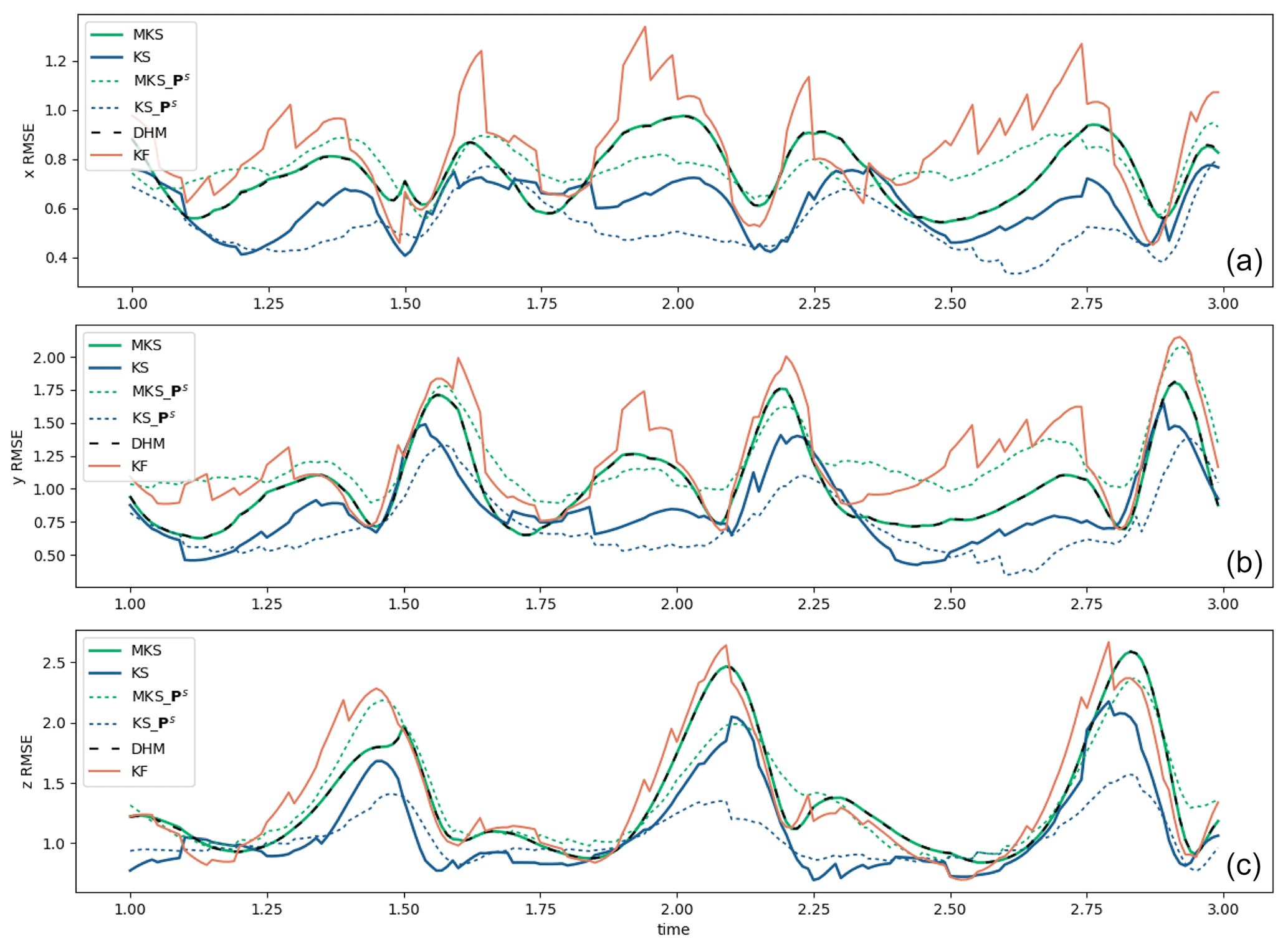
Figure 1The RMSE time series for the KF and KS, along with the MKS and the DHM smoother, in the L63 system for (a) x, (b) y, and (c) z. The RMSEs are averaged across 100 independent assimilation runs starting from different initial conditions and assimilating observations from the same 20 time unit truth run. Only two time units of the run are shown to allow the behaviour around the analysis times to be clearly seen. Dotted green lines and dotted blue lines (see the panel insets for details) are the posterior uncertainty SD (square root of error covariance P) estimates for the MKS and KS, respectively.
The time mean RMSEs for are summarised in Table 1, along with the uncertainty SD, where calculated, over the entire 20 time units of the runs. Both DHM and MKS provide an improvement on the ExtKF results by 60 %–70 %, relative to the ExtKS improvements for x and y, although the RMSE for z is not reduced in DHM and MKS. This is perhaps because the instantaneous error covariances between z and the assimilated x,y variables, as used in DHM, are insufficient to improve z, whereas the full ExtKS allows some history of the x,y evolution to be used for deriving z smoothing increments. The RMSE numbers in parentheses are evaluated only at the filter update time steps, where observation data are assimilated. These errors are smaller than all-time-step RMSEs by ∼ 5 %, which is as a result of the data assimilation at these time steps. This is consistent with the RMSE time series in Fig. 1, where the Kalman filter (orange line) usually declines sharply when data are available. The smoother solutions, however, also yield much-improved analyses between observation time steps.
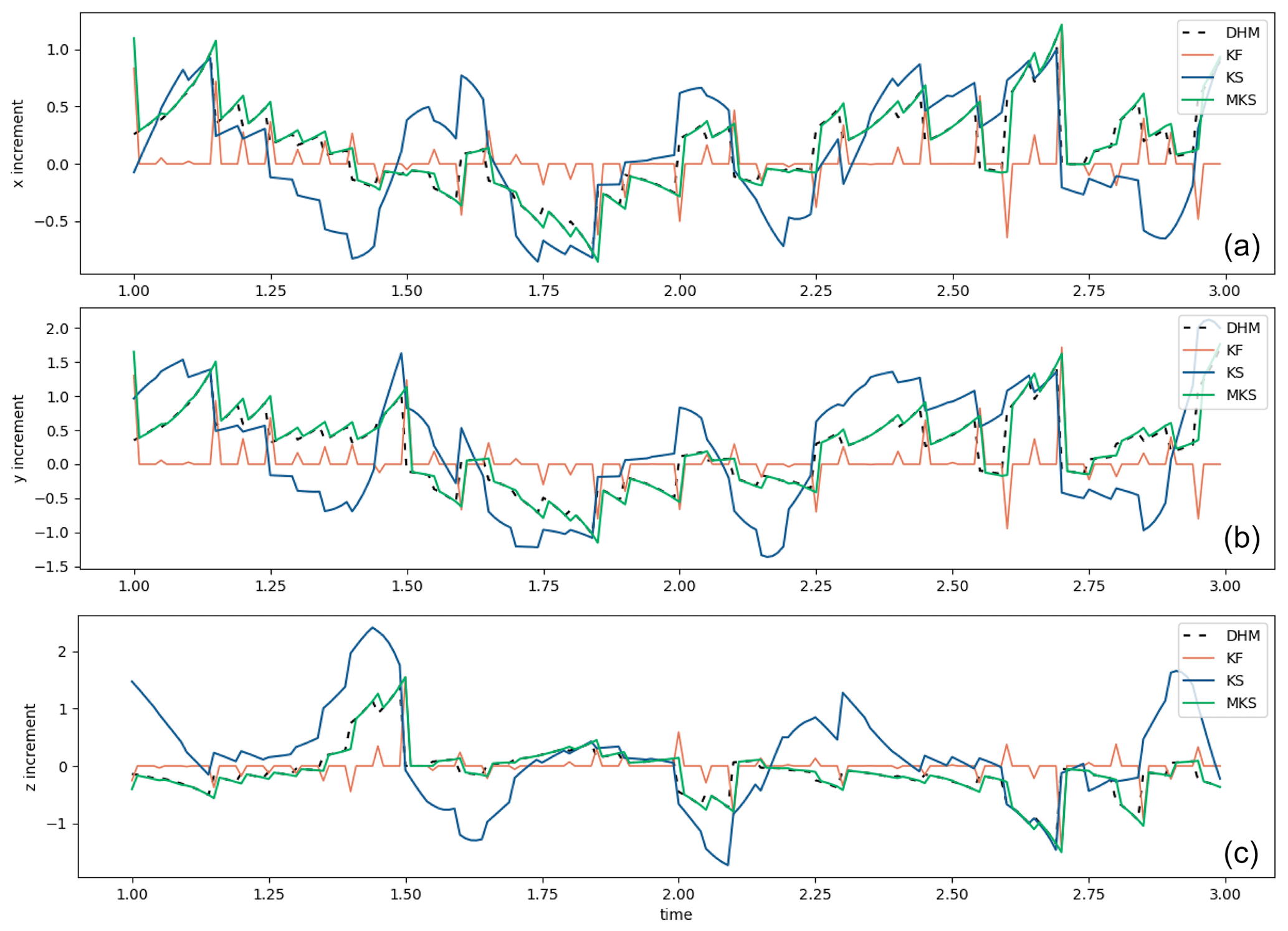
Figure 2As in Fig. 1 but the filter and smoother increments are shown for situations where the smoother increments, when applied, add to the filter increments.
Figure 2a, b, and c show the actual increments, respectively, being introduced by the ExtKF and the different smoothers through the analysis times. In each case, the smoother increments are additional to the filter increments, which appear clearly as orange spikes for every five time steps when data are available. Smoother increments between analysis times can be seen, with the DHM and MKS increments being virtually identical and decaying backwards in time from each filter increment. The ExtKS increments are more complex, sometimes being similar to the DHM, but sometimes they can be considerably larger.
If we look at the mean ratio of the cross-time error covariances relative to the filter forecast error covariances in comparison to the simplified γ decay representation across time in Fig. 3, we can understand something about the performance of the smoothers. We do not expect these to be identical because the full cross-time smoother covariances for larger lags, ℓ, take account of the increments from intermediate times. For small lag values, the average cross-time error decay rates are fairly similar; however, for larger lag values, the model-derived cross-time error covariance on average takes the opposite sign. This happens on a similar timescale to the short oscillation period of x,y in L63 and is associated with the growing amplitude of these oscillations as they reach larger and smaller x,y values before the phase lobe transitions. This is a very model-specific behaviour, and the simple smoother's γ decay error covariances cannot represent this. This also explains why larger γ values make the simple smoother worse in L63 because the positive cross-time error covariances are used for larger lags when the negative cross-time error covariances are more appropriate.
The key point is that the simplified smoother DHM provides substantial improvement over the ExtKF, while incurring very little computational cost (no tangent linear model or TLM runs and no storage of cross-time error covariances) compared to the ExtKS. The DHM smoother can therefore be applied in its entirety through the post-processing of the filter results. While this was demonstrated in Dong et al. (2021), here we show more clearly how the equivalent MKS approximation is derived from the ExtKS equations, and we also show how the smoothed uncertainties can be cheaply post-processed and still give useful information.
In the next section, we extend the decay assumption for cross-time error covariances to apply to the ensemble Kalman filter and smoother equations, which are much more relevant to large nonlinear models for which the direct modelling of error covariances across time is infeasible.
Table 1Time mean RMSE against truth for the ExtKF and ExtKS, along with the modified MKS and the simplified DHM smoother for each variable in the L63 system (see also legend for Fig. 1). The numbers in parentheses are the mean RMSE values at observation time steps only (not independent data). The time mean of the standard deviations calculated for the uncertainties are also shown as SD. Time averaging is now over the entire 20 time units of each assimilation run.
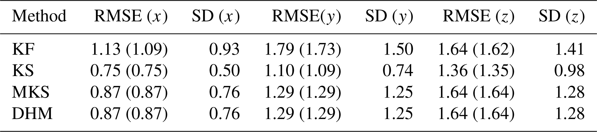
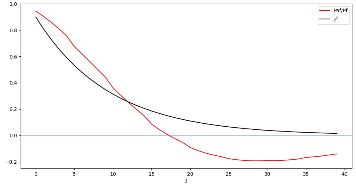
Figure 3Cross-time error covariance decay rates for the ExtKS and the DHM smoother. For the ExtKS, the y axis is the smoother cross-time error covariance divided by the filter forecast error covariance and averaged for all times over the 20 time unit L63 run. This is compared to the decay of γℓ used in the DHM smoother, as a test of Eq. (12).
4.1 Approximating ensemble error covariances
In the ExtKF and ExtKS, a TLM propagates the flow-dependent error statistics, which are then used to calculate increments. However, the TLM reliability declines sharply with propagation time for a system as nonlinear as the L63 model. The ensemble Kalman filter (EnKF) can then give better results by estimating the error statistics with a finite ensemble of state realisations propagated by the full nonlinear model rather than by a TLM. This can then improve the quality of the forecast error covariance matrix. However, the update gains for the EnKF and ensemble Kalman smoother (EnKS) are defined identically to Eqs. (7) and (9), respectively, although the error covariances, (the error covariance at time step k) and (the error covariance between time steps k and k+ℓ) are calculated differently, since they are emulated from the limited ensemble of state vectors whose variability represents the uncertainty in the system. While ensemble filter methods have been adopted for larger environmental models, these have not generally added smoother steps because the cost to store, update, and apply posterior ensemble covariances still makes ensemble smoother methods generally infeasible.
However, these constraints can again be overcome by retaining the EnKF flow-dependent ensemble spreads to represent current errors, while making a simple decay approximation for the time shift error covariances, which is similar to our modified ExtKS in Sect. 2.2. For comparison purposes, we demonstrate this method in the general EnKS form in state space, keeping the same notation as we used previously, although the actual computation is performed in ensemble space, as in the ensemble transform Kalman filter (ETKF; e.g. Bishop et al., 2001; Zeng and Janjić, 2016).
where
is the normalised anomaly of the ith ensemble member from the mean in an Ne member ensemble of forecasts.
The first step in the ensemble filter is to update the ensemble mean,
and the second step is to update the uncertainty, using Eq. (8). Then, in order to regenerate the ensemble of analysis perturbations, the ETKF uses the following transformation:
where Tk is chosen to ensure that Eq. (8) is satisfied. Then, following the EnKF, the cross-time covariances in the EnKS can be expressed in state space as follows:
As explained in the Appendix, the full cross-time error covariances are calculated between the filter forecast ( in the EnKS) and previous partially smoothed states (Xk again in the EnKS), which require both past ensemble means and error covariances to be repeatedly smoothed. However, this is not necessary for the modified (simple) ensemble smoother, which we here call MEnKS. The ensemble mean smoothing using Eqs. 13 and 10 can be written as follows:
and then Eq. (18) can be used to obtain the smoothed uncertainties.
This is a great simplification because performing a full ensemble smoothing would require the whole past ensemble to be stored at all times and reprocessed. Equation (19) suggests that the error covariance increments must also be stored during the EnKF filter phase, which could still be a large storage requirement for a big model; however, in fact only the diagonal elements of Ps are likely to be of interest, i.e. the uncertainty variance of the state fields, or even just a subset of these, so only a smaller set of uncertainty increments may be of interest and worth storing for post-processing through Eq. (19). In the next subsection, we show the results of applying these approximations in L63.
4.2 EnKS assimilation results
Using the same L63 twin experiment as in Sect. 3, we solve a full smoother (EnKS) and use the modified (MEnKS) algorithm Eq. (28). To be consistent with the extended KS configuration, we use an ensemble size of 100 and a fixed lag of 40 time steps for smoothing. Figure 4a, b, and c show the RMSE and SD uncertainties, respectively, from these ensemble filter and smoother runs in the same format used in Fig. 1 for the extended Kalman filter.
These ensemble results are seen to produce lower RMSE values than the equivalent ExtKF or KS results (cf. Fig. 1), demonstrating the superiority of the ensemble assimilation method for dealing with the nonlinearity of the L63 model. Again, the EnKS substantially reduces the RMSE compared to the filter, and again, the approximated simple ensemble filter MEnKS gives intermediate RMSE results, with much less computational effort than the full EnKS. Although not as optimal as the EnKS, the simplified MEnKS shows a much smoother temporal evolution of the RMSE than the filter, which would be a significant improvement if, for example, applied to an ocean reanalysis. The post-processed uncertainty estimates also reproduce a reasonable estimate of the true RMSEs of the smoothed ensemble mean analyses.
Figure 5a, b, and c show the mean increment time series, respectively, for the ensemble filter and the two smoothers. The increments are smaller than those from the ExtKF/KS (Fig. 2), reflecting the improved assimilation approaches. Table 2 summarises the average RMSE and SD uncertainty results over the full 20 time units of the ensemble runs.
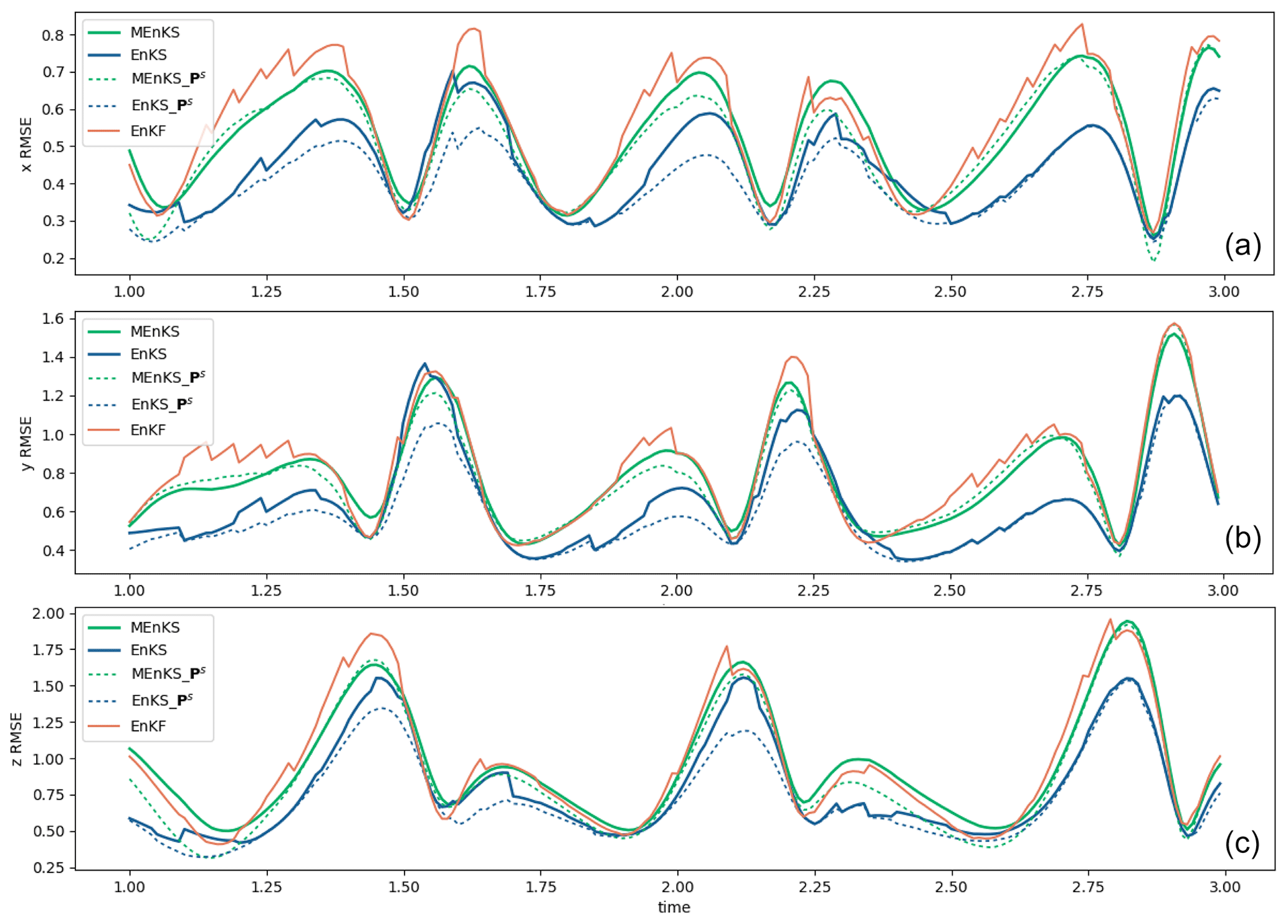
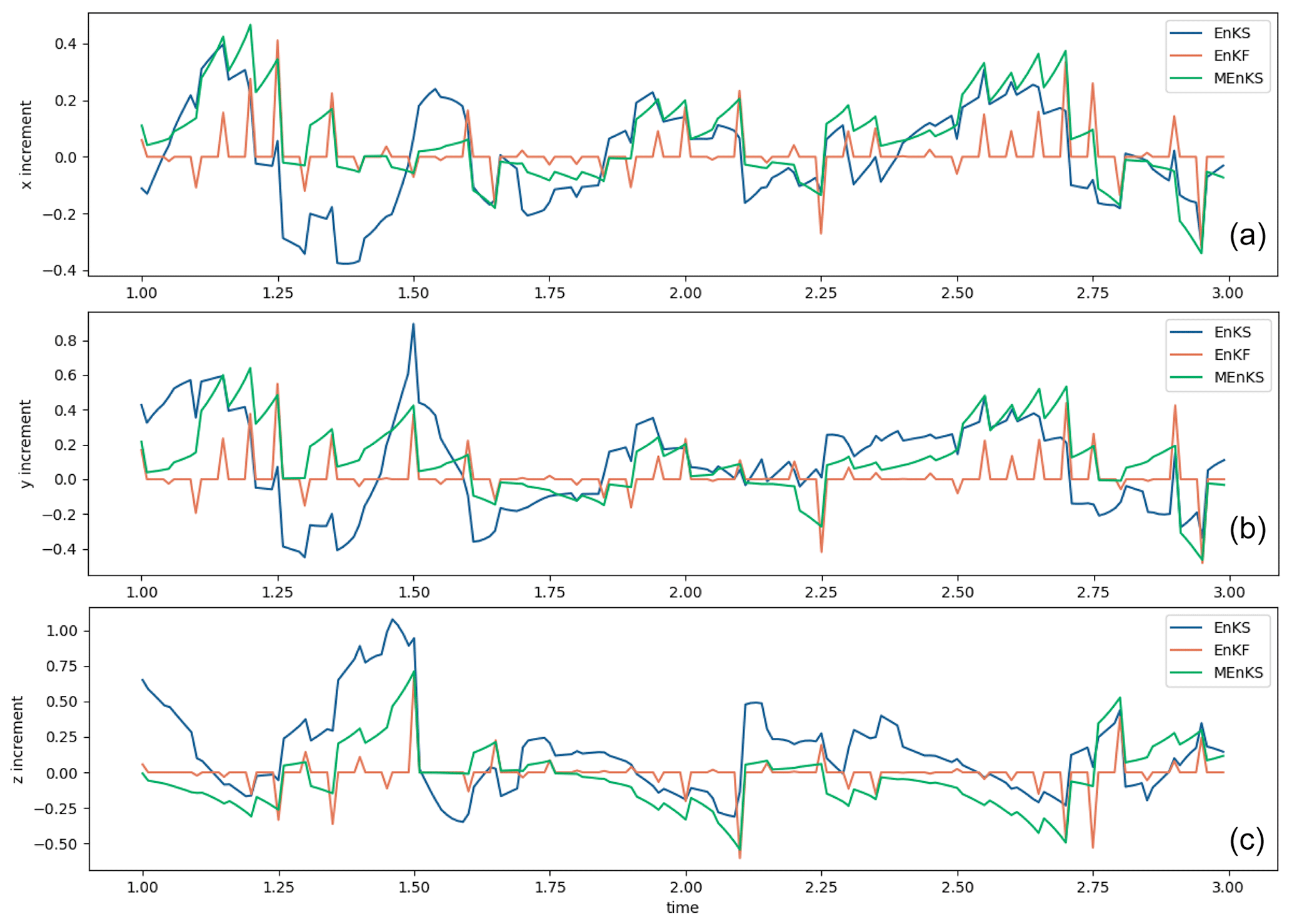
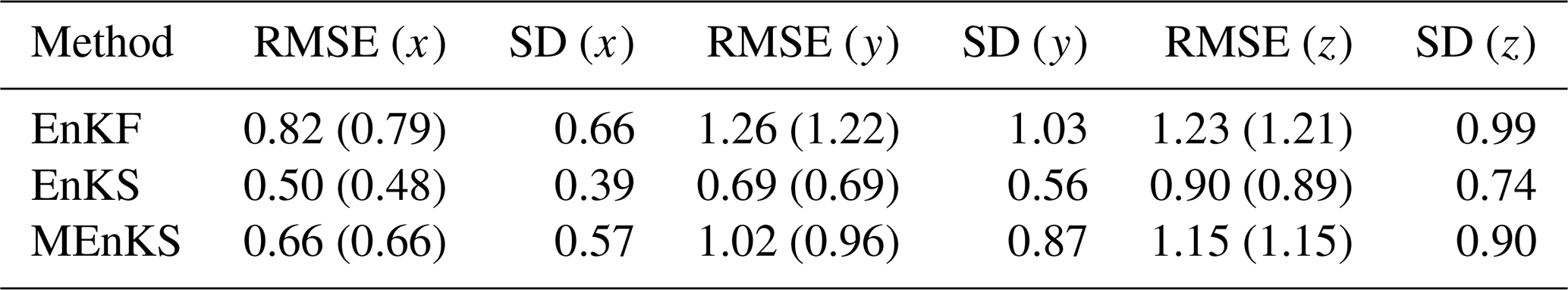
Table 2Time mean RMSE and SD uncertainties for each variable in EnKF, EnKS, and MEnKS in the L63 model, averaged over time units from 1–20. The numbers in parentheses are the RMSE values calculated at time steps with observations only (no independent data comparison). The lag is 40, and γ=0.9.
The aim of this paper is clearly not to present an improved data assimilation approach for simple models but to explore traceable simplifications to the current assimilation approaches which could be applied to high-dimensional models. In particular, ocean and Earth system models are starting to be used for the reanalysis of past climate states, using essentially the same codes that have been developed for operational forecasting and especially of the atmosphere (i.e. sequential filter codes). Even when 4D-Var approaches are being used, e.g. at ECMWF, the effective temporal smoothing window timescales are generally short, reflecting the validity of the tangent linear and adjoint modelling for the atmosphere. In these cases, Kalman smoothing approaches could still yield tangible benefits, especially for long timescale process variables associated with the Earth system and when reanalysing by using sparse historical observing systems.
However, there are still further challenges to applying smoother algorithms in really large systems. In Dong et al. (2021), the simple smoother was applied to an ocean reanalysis, and it was found that the smoothed analysis gave reduced errors compared to the filter when compared against independent, unassimilated data. However, it was also noted that problems can occur when observations or model are biased. Biased increments can be detected when the same increment is repeatedly produced by the filter, which is a signal that the model is unable to retain the information. While this may not invalidate the filter analysis, it could have a very detrimental impact on the smoothing when multiple versions of the same increment may be added without the model being rerun. While bias can be allowed for if it is identified prior to the smoothing, any real application of smoothing needs to consider this carefully. This is perhaps another reason to prefer smoothing as a post-processing step, when bias assessments can be made beforehand, rather than as an integrated part of a sequential forward analysis, as it is usually presented in the literature (Todling and Cohn, 1996; Evensen and van Leeuwen, 2000; Bocquet and Sakov, 2014).
Another option not explored here, because L63 is too simple, is the ability to tune the γ decay timescale according to different state variables. In Dong et al. (2021), this was suggested as allowing the subsurface ocean increments to decay more slowly than the surface increments, for example. In the notation used here, γ would then become a diagonal decay matrix multiplying the forecast error covariance to convert to a cross-time error covariance.
A key benefit to smoothing in real systems would be to bring the influence from observations made in the near future, when none has been available in the near past, for instance, after the deployment of new observing platforms. A key difference between using our approach and using a full smoother is that in a full smoother the cross-time error covariances depend upon observations previously assimilated within the smoothing lag time window (see the Appendix). Thus, a full smoother will reduce the analysed error covariances due to the influence of the short lag future data first and will therefore reduce the cross-time error covariances to be applied for longer lag future data, thus ensuring that the most important near-future data have the biggest smoothing influence. This reduction in longer lag influences if shorter lag data are available is missing in the simple smoother as presented here and could cause the application of the smoother to give poorer results when very frequent observations are available. Further simple modifications that can take this into account could be envisioned, for example, by allowing γ to reflect upgrades in the observing network during the period of the reanalysis. Alternatively, uncertainty reduction information for each future increment, as estimated through Eq. (19), could be used to truncate or reduce γ for the smoothing of longer lag increments through Eq. (15).
Although we have proposed how these ideas could be used in ensemble systems, we have not explored the other challenges of using ensembles in large model products. In particular, localisation is often required to remove unrealistic error covariances arising from limited ensemble sizes (e.g. Petrie and Dance, 2010). When extended to ensemble smoothing, then that localisation may need to vary with the lag for the cross-time error covariances (e.g. Desroziers et al., 2016). When faced with such challenges, the simple smoothing method is at least explicit in its assumption that the spatial structure of the error covariances are static, while guaranteeing that the cross-time error covariances will always decay away with time.
We have included the smoothing of uncertainty estimates in the analysis here, despite the fact that these have rarely been attempted for previous large model reanalysis products – even when only forward-filtering steps are involved. However, with the recent trend towards ensemble analysis products, for both operational and reanalysis systems, it makes sense to ask how well the uncertainty estimates correspond to the errors in an idealised system where this can be evaluated against, for example, independent data. At the same time, we have demonstrated the ability to evaluate smoother uncertainty estimates, and we have found these results very encouraging.
We have demonstrated that both the extended Kalman smoother and the ensemble Kalman smoother can be simplified to use only a relatively small amount of information stored during a forward-filtering analysis. This permits the simple smoothing approach to be applied through post-processing. The essential novelty is to treat cross-time error covariance information as decaying exponentially on some tuneable timescale, rather than seeking to calculate these covariances with the system model. This allows the stored state increments to be down-weighted and added to previous filter analyses. We also show how the smoother uncertainty information can be post-processed, provided the increments (changes) in the error covariances between the forecast and analysis for each filter assimilation window are stored. And we note that the error variance of the state fields alone could be smoothed, meaning that only one additional state field needs to be stored from each filter analysis.
The method has been demonstrated, using the assimilation runs of the L63 model and using the same idealised assimilated data over a 20 time unit truth run when starting the model from different initial conditions. Observational, but not model, errors are being simulated. In both the extended and ensemble Kalman smoother cases, using the full smoother equations gives the best RMSE results against the truth. However, in each case, the simple smoother method still gives substantially reduced RMSE values compared with the respective Kalman filters, e.g. ∼ 70 % of the error reduction in the extended Kalman smoother. We also include the RMSE evaluated only at filter analysis times, when the truth comparison data are not independent (observations from these times, albeit with added errors, have been assimilated), and still find that the smoother results provide substantial improvements over the filter. We include these comparisons because operational systems do not usually hold back independent data for assessment. The ensemble filter/smoother results are substantially better than the extended filter/smoother results, as would be expected for such a nonlinear system as L63. The simple smoother retains this benefit, as the flow-dependent ensemble filter error covariances are retained, although down-weighted, for the smoother's cross-time errors covariances.
We also demonstrate the smoothing of the uncertainty estimates in both the ExtKS and EnKS systems. Remarkably, the uncertainty estimates, presented as the SDs of the smoother state variances, are in very good agreement with the RMSE errors being calculated against the truth. The uncertainties rise and fall over time, similar to the RMSEs, as the model moves through the more stable and unstable regions of the phase space. Uncertainty estimates are usually a little lower than the calculated RMSE values. The simple smoothing approach gives higher uncertainties than the full smoother estimates but is in excellent agreement with the simple smoother RMSE values.
We believe that this approach offers a feasible offline post-processing approach for improving reanalyses in really large Earth system models. An initial paper with the first results from smoothing the Met Office ocean reanalysis using stored increments was presented in Dong et al. (2021). This paper demonstrates the traceable origin of the approach from Kalman filtering roots and puts the method in a wider context, including showing how it can be used in ensemble systems that are just starting to be used operationally in order to obtain better representations of uncertainty.
We summarise the post-processing requirements that would allow the smoothing of large model datasets as follows.
-
If increments from the sequential filter analysis are stored, then this should be sufficient to allow the post-processing of a smoother solution.
-
If an ensemble product is being generated, then only the ensemble mean fields and ensemble mean increments would be needed to obtain a smoothed ensemble mean solution.
-
If an uncertainty estimate is also needed for the smoother solution, then the minimum additional requirement would be to store the increments of those components of the error covariance matrix of interest. This may consist of the error variances of each state field or only a subset of state fields, e.g. only surface fields from an ocean model.
-
If uncertainty information from an ensemble product is required, then the minimum additional storage requirement would still only be the filter increments in the error covariance components of interest. The whole past ensemble analyses would not be needed.
In order to show formally how our simple smoother system in Sect. 2.1 is related to the classical Kalman smoother, we start with a brief summary of the Kalman filter (KF) and fixed-lag Kalman smoother (KS) formulations. We base our system of equations on Todling and Cohn (1996, hereafter TC96), which we use as our reference for the classical smoother. We therefore adopt a notation similar to theirs. This is a more complex notation than that of the main part of this paper but is useful for complete traceability.
A1 Background to the Kalman filter and smoother
The analysis of the KF at time k and its error covariance are given by
Here the subscript indicates that the object is valid at time step k and has been formed from observations up to and including time step k−1. States and are the forecast state and filter analysis, respectively, at validity time k, where has been evolved by the model ℳ, e.g. . The forecast state error covariance may be evolved by the model (as in the extended KF) or obtained from an ensemble of model state forecasts (ensemble KF), but either way, the analysis error covariance Eq. (A2) for is obtained. The vector yk represents the observations at k, whose model counterparts are found using the observation operator ℋk via , and Hk is the tangent linear operator of ℋk. Rk is the observation error covariance matrix, and Kk|k is the Kalman gain. Equations (A1), (A2), and (A3) are the same equations as Eqs. (6), (8), and (7), respectively, in the main paper but use the TC96 notation.
For the classical fixed-lag KS of maximum lag L, an interval of L+1 time steps are updated together after every filter time step. These L+1 states are valid for time steps k, and are to be updated by observations at time step k. This is the backward-looking scheme of TC96, which runs interleaved with the filter (below we use j to represent the backward-looking intervals). Prior to this update – and using a similar notation to TC96 – these states are , , … , . These are shown as the black states in Fig. A1a. At this point, only observations up to k−1 have been assimilated, which is reflected in the notation, and so superscript “a” refers to partially smoothed analyses generated only using observations up to time k−1. The state is the pure k−1 filter analysis, and is the filter forecast at k derived from it. The covariances of, and between, these states are the black block matrices in Fig. A1b, which are used to form the gain matrices in the current update (below).
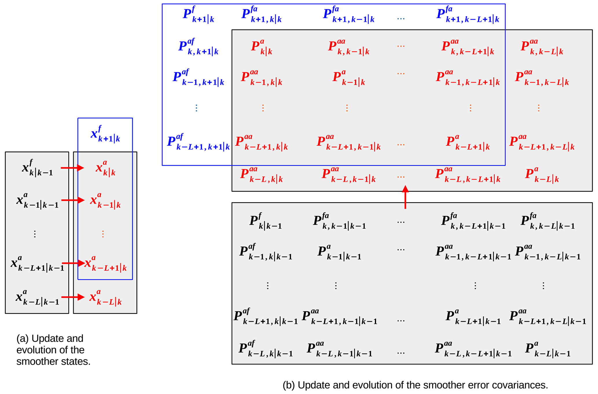
Figure A1Schema of the fixed-lag KS of TC96. Panel (a) shows the update and evolution of the set of states within the fixed-lag interval of L+1 time steps. The smoother update starts with the set of states in black, which are updated (or smoothed) by observations at k to the set of states in red, using Eq. (A1) for the most recent state (at the top) and Eq. (A4) for the remainder. The subscripts have the form k|p, where k is the state's validity time, and p is the time step of the latest observations that have contributed to estimating that state. The Kalman gains (Eqs. A3 and A6) rely on knowledge of the covariances in panel (b), with reference to the first column of the black matrix. The lag interval then progresses by one time step (blue box in panel a), where the forecast (blue state) is evolved from the latest analysis using the model. Panel (b) shows the update and evolution of the error covariances within the fixed-lag interval. The black matrix blocks are the error covariances of the set of black states in panel (a). The diagonal blocks have a subscript with the same form as the states, but the off-diagonal blocks have subscripts of the form , which correspond to cross-covariances between time steps k and k′. The smoother updates the black covariances to the red covariances, using equations not fully shown in this paper (see Eqs. 37, 39, and 41 of TC96, which use information from the black matrices). The lag interval then progresses, as it does for the states, by one time step (blue box), where the extra covariances (blue) are propagated from the red covariances using Eqs. (46) and (47) of TC96 and the tangent linear model.
The fixed-lag KS determines how observations at k update the states at the previous time levels to give , , … , (the red states in Fig. A1a), and their covariances (the red matrices in Fig. A1b). The first state, , and its covariance, , are updated using the KF equations, but the remaining states, , and their covariances, () are updated by the KS equations as follows:
The new objects are , the updated smoothed state at k−j due to observations at k, and the corresponding updated covariance. Both objects are obtained using , which is the gain for the smoother state at k−j due to observations at k.
To make these updates requires a new kind of covariance for errors between different times. These have a subscript of the form , which indicates that the covariance is between the time steps k and k′ and has been formed from information up to and including time step k−1. In the above, are the covariances between errors in and . Each is obtained from in Fig. A1b as separate covariance propagations (or from an ensemble of forecasts in the EnKS) for each k−j. If the EnKS is being used, then these error covariances are not derived directly but require all the partially smoothed ensemble members within the lag L to be retained. These are the same covariances as those expressed in Eq. (27) in the main text's truncated notation.
Equation (A4) is a version of TC96's Eq. (26), Eq. (A5) is their Eq. (39), and Eq. (A6) is their Eq. (35). Notice that the same error covariance matrix, , appears in the parentheses in Eqs. (A3) and (A6). The incremental part of Eq. (A5) is the same as Eq. (16) in the main paper, and Eq. (A6) is the same as Eq. (11) but using the TC96 notation here. There is no equivalent for Eq. (A4) given in the main paper. The KS system is advanced by one time step by propagating , using the model, to (the blue state in Fig. A1a), giving a shifted interval of states (blue box in Fig. A1a). The covariances are propagated by the tangent linear model (the blue block matrices in Fig. A1b) or by propagating the ensemble of the new analyses, giving a shifted interval of covariances (blue box in Fig. A1b).
A2 Equations for maximally smoothed states and covariances and equivalence to the simple smoother
Given the maximum lag, L, the sequence of states (and their error covariances ) exploit the maximum amount of observational information, as they have been updated with all L+1 sets of present and future observations. These are the states that are analogous to in Sect. 2.1. For a general k, the fully smoothed states here are , which can be found from cyclic application of the KS equations. By recursively applying Eq. (A4) over the lag window, it is straightforward to find the following explicit full smoothing solution (where the superscript “s” is used in main text) in a forward-looking perspective (with ℓ to represent forward-looking intervals; cf. Eq. 10 in the main paper).
Similarly, recursively applying Eq. (A5) over the lag window leads to the following explicit covariance of this fully smoothed estimate (cf. Eq. 17):
We will now use Eqs. (A7) and (A8) to show the necessary approximations needed to give the simplified smoothing equations shown in Sects. 2.1 and 2.2.
The fundamental approximation is applied to the cross-time error covariances (as they appear in Eq. A6), using a temporal covariance decay and writing the following (cf. Eq. 12):
This is equivalent to writing , using Eqs. (A6) and (A3), as follows (cf. Eq. 13):
Equation (A10) is in a forward-looking form, allowing it to be used in Eq. (A7).
where the last line follows from the first using the filter, Eq. (A1), and allowing us to relate the simplified smoother updates to the later filter increments. Equation (A11) is analogous to the simplified scheme of Eq. (1), where is the post hoc smoothing analysis (S0 in Eq. 1), is the previous filtering analysis (A0), and the terms in parentheses form the filter analysis increments at future times (Ij). Also compare this information to Eq. (15).
It is possible to make the equivalent approximations to the smoothed covariances in Eq. (A8). Using Eqs. (A9) and (A10) gives
From Eq. (A2), in the above is equal to the difference between the forecast and filter analysis error covariance matrices, making the above
This is the same as Eq. (19) in the main body of the paper except for using the TC96 notation.
Implementations of the L63 system for the ExtKF and ExtKS codes and the EnKF and EnKS codes are available on Zenodo (https://doi.org/10.5281/zenodo.7675286; Dong and Chen, 2023). The implementation here is based on the Python-based data assimilation templates of DAPPER (https://github.com/nansencenter/DAPPER, last access: 24 February 2023, https://doi.org/10.5281/zenodo.2029296, Raanes et al., 2018).
BD and KH initiated the research idea and designed the experiments. All authors contributed to the theoretical developments presented. BD and YC implemented the codes and developed the diagnostic results. All authors contributed to the writing of the paper.
The contact author has declared that none of the authors has any competing interests.
Publisher's note: Copernicus Publications remains neutral with regard to jurisdictional claims in published maps and institutional affiliations.
All authors acknowledge support from the NERC NCEO LTSS strategic programme DA project for their contributions to this work. We also thank Guokun Lyu and two anonymous reviewers for their careful review and constructive comments.
This research has been supported by the National Centre for Earth Observation through UKRI NERC funding (grant no. NE/R016518/1).
This paper was edited by Yuefei Zeng and reviewed by Guokun Lyu and two anonymous referees.
Balmaseda, M. A., Mogensen, K., and Weaver, A. T.: Evaluation of the ECMWF ocean reanalysis system ORAS4, Q. J. Roy. Meteor. Soc., 139, 1132–1161, 2013. a
Bishop, C. H., Etherton, B. J., and Majumdar, S. J.: Adaptive Sampling with the Ensemble Transform Kalman Filter. Part I: Theoretical Aspects, Mon. Weather Rev., 129, 420–436, https://doi.org/10.1175/1520-0493(2001)129<0420:ASWTET>2.0.CO;2, 2001. a, b
Bocquet, M. and Sakov, P.: An iterative ensemble Kalman smoother, Q. J. Roy. Meteor. Soc., 140, 1521–1535, https://doi.org/10.1002/qj.2236, 2014. a, b
Buizza, R., Poli, P., Rixen, M., Alonso-Balmaseda, M., Bosilovich, M. G., Brönnimann, S., Compo, G. P., Dee, D. P., Desiato, F., Doutriaux-Boucher, M., Fujiwara, M., Kaiser-Weiss, A. K., Kobayashi, S., Liu, Z., Masina, S., Mathieu, P.-P., Rayner, N., Richter, C., Seneviratne, S. I., Simmons, A. J., Thépaut, J.-N., Auger, J. D., Bechtold, M., Berntell, E., Dong, B., Kozubek, M., Sharif, K., Thomas, C., Schimanke, S., Storto, A., Tuma, M., Välisuo, I., and Vaselali, A.: Advancing Global and Regional Reanalyses, B. Am. Meteorol. Soc., 99, ES139–ES144, https://doi.org/10.1175/BAMS-D-17-0312.1, 2018. a
Burgers, G., Van Leeuwen, P. J., and Evensen, G.: Analysis scheme in the ensemble Kalman filter, Mon. Weather Rev., 126, 1719–1724, 1998. a
Cosme, E., Brankart, J.-M., Verron, J., Brasseur, P., and Krysta, M.: Implementation of a reduced rank square-root smoother for high resolution ocean data assimilation, Ocean Model., 33, 87–100, https://doi.org/10.1016/j.ocemod.2009.12.004, 2010. a
Desroziers, G., Arbogast, E., and Berre, L.: Improving spatial localization in 4DEnVar, Q. J. Roy. Meteor. Soc., 142, 3171–3185, 2016. a
Dong, B. and Chen, Y.: code for paper “Simplified Kalman smoother and ensemble Kalman smoother for improving ocean forecasts and reanalyses”, Zenodo [code], https://doi.org/10.5281/zenodo.7675286, 2023. a
Dong, B., Haines, K., and Martin, M.: Improved high resolution ocean reanalyses using a simple smoother algorithm, J. Adv. Model. Earth Sy., 13, e2021MS002626, https://doi.org/10.1029/2021MS002626, 2021. a, b, c, d, e, f, g, h, i, j, k, l
Evensen, G.: Sequential data assimilation with a nonlinear quasi-geostrophic model using Monte Carlo methods to forecast error statistics, J. Geophys. Res.-Oceans, 99, 10143–10162, https://doi.org/10.1029/94JC00572, 1994. a
Evensen, G.: The ensemble Kalman filter for combined state and parameter estimation, IEEE Contr. Syst. Mag., 29, 83–104, https://doi.org/10.1109/MCS.2009.932223, 2009. a
Evensen, G. and van Leeuwen, P. J.: An Ensemble Kalman Smoother for Nonlinear Dynamics, Mon. Weather Rev., 128, 1852–1867, https://doi.org/10.1175/1520-0493(2000)128<1852:AEKSFN>2.0.CO;2, 2000. a, b
Evensen, G., Vossepoel, F. C., and van Leeuwen, P. J.: Data assimilation fundamentals: A unified formulation of the state and parameter estimation problem, Springer Nature, ISBN 9783030967093, 9783030967093, https://doi.org/10.1007/978-3-030-96709-3, 2022. a
Feng, L., Palmer, P. I., Bösch, H., and Dance, S.: Estimating surface CO2 fluxes from space-borne CO2 dry air mole fraction observations using an ensemble Kalman Filter, Atmos. Chem. Phys., 9, 2619–2633, https://doi.org/10.5194/acp-9-2619-2009, 2009. a
Hamill, T. M., Whitaker, J. S., Fiorino, M., and Benjamin, S. G.: Global ensemble predictions of 2009’s tropical cyclones initialized with an ensemble Kalman filter, Mon. Weather Rev., 139, 668–688, 2011. a
Houtekamer, P. L. and Mitchell, H. L.: Data assimilation using an ensemble Kalman filter technique, Mon. Weather Rev., 126, 796–811, 1998. a
Houtekamer, P. L., Mitchell, H. L., Pellerin, G., Buehner, M., Charron, M., Spacek, L., and Hansen, B.: Atmospheric Data Assimilation with an Ensemble Kalman Filter: Results with Real Observations, Mon. Weather Rev., 133, 604–620, https://doi.org/10.1175/MWR-2864.1, 2005. a
Khare, S. P., Anderson, J. L., Hoar, T. J., and Nychka, D.: An investigation into the application of an ensemble Kalman smoother to high-dimensional geophysical systems, Tellus A, 60, 97–112, https://doi.org/10.1111/j.1600-0870.2007.00281.x, 2008. a
Lorenz, E. N.: Deterministic nonperiodic flow, J. Atmos. Sci., 20, 130–141, 1963. a, b, c, d, e
MacLachlan, C., Arribas, A., Peterson, K. A., Maidens, A., Fereday, D., Scaife, A. A., Gordon, M., Vellinga, M., Williams, A., Comer, R. E., Camp, J., Xavier, P., and Madec, G.: Global Seasonal forecast system version 5 (GloSea5): A high-resolution seasonal forecast system, Q. J. Roy. Meteor. Soc., 141, 1072–1084, 2015. a
Pan, Y., Zhu, K., Xue, M., Wang, X., Hu, M., Benjamin, S. G., Weygandt, S. S., and Whitaker, J. S.: A GSI-Based Coupled EnSRF–En3DVar Hybrid Data Assimilation System for the Operational Rapid Refresh Model: Tests at a Reduced Resolution, Mon. Weather Rev., 142, 3756–3780, https://doi.org/10.1175/MWR-D-13-00242.1, 2014. a
Petrie, R. E. and Dance, S. L.: Ensemble-based data assimilation and the localisation problem, Weather, 65, 65–69, 2010. a
Pinnington, E., Quaife, T., Lawless, A., Williams, K., Arkebauer, T., and Scoby, D.: The Land Variational Ensemble Data Assimilation Framework: LAVENDAR v1.0.0, Geosci. Model Dev., 13, 55–69, https://doi.org/10.5194/gmd-13-55-2020, 2020. a
Raanes, P. N., Grudzien, C., and 14tondeu: nansencenter/DAPPER: Version 0.8 (v0.8), Zenodo [code], https://doi.org/10.5281/zenodo.2029296, 2018. a
Ravela, S. and McLaughlin, D.: Fast ensemble smoothing, Ocean Dynam., 57, 123–134, https://doi.org/10.1007/s10236-006-0098-6, 2007. a
Sakov, P., Counillon, F., Bertino, L., Lisæter, K. A., Oke, P. R., and Korablev, A.: TOPAZ4: an ocean-sea ice data assimilation system for the North Atlantic and Arctic, Ocean Sci., 8, 633–656, https://doi.org/10.5194/os-8-633-2012, 2012. a
Skachko, S., Ménard, R., Errera, Q., Christophe, Y., and Chabrillat, S.: EnKF and 4D-Var data assimilation with chemical transport model BASCOE (version 05.06), Geosci. Model Dev., 9, 2893–2908, https://doi.org/10.5194/gmd-9-2893-2016, 2016. a
Todling, R. and Cohn, S.: Some strategies for Kalman filtering and smoothing., in: Proc. ECMWF Seminar on data assimilation, 91–111, 1996. a, b, c, d
Uppala, S. M., Kållberg, P., Simmons, A. J., Andrae, U., Bechtold, V. D. C., Fiorino, M., Gibson, J., Haseler, J., Hernandez, A., Kelly, G., and Woollen, J.: The ERA-40 re-analysis, Q. J. Roy. Meteor. Soc., 131, 2961–3012, 2005. a
van Velzen, N., Altaf, M. U., and Verlaan, M.: OpenDA-NEMO framework for ocean data assimilation, Ocean Dynam., 66, 691–702, 2016. a
Wang, X., Parrish, D., Kleist, D., and Whitaker, J.: GSI 3DVar-based ensemble–variational hybrid data assimilation for NCEP Global Forecast System: Single-resolution experiments, Mon. Weather Rev., 141, 4098–4117, 2013. a
Whitaker, J. S. and Hamill, T. M.: Ensemble data assimilation without perturbed observations, Mon. Weather Rev., 130, 1913–1924, 2002. a
Zeng, Y. and Janjić, T.: Study of conservation laws with the local ensemble transform Kalman filter, Q. J. Roy. Meteor. Soc., 142, 2359–2372, 2016. a
Zhang, M. and Zhang, F.: E4DVar: Coupling an ensemble Kalman filter with four-dimensional variational data assimilation in a limited-area weather prediction model, Mon. Weather Rev., 140, 587–600, 2012. a
Zhu, Y., Todling, R., Guo, J., Cohn, S. E., Navon, I. M., and Yang, Y.: The GEOS-3 Retrospective Data Assimilation System: The 6-Hour Lag Case, Mon. Weather Rev., 131, 2129–2150, https://doi.org/10.1175/1520-0493(2003)131<2129:TGRDAS>2.0.CO;2, 2003. a, b
- Abstract
- Introduction
- Methods
- Extended Kalman smoother experiments in the L63 system
- Ensemble Kalman smoother experiments in the L63 system
- Discussion
- Conclusions
- Appendix A: Formal derivation of the simple smoother system from the Kalman filter and Kalman smoother equations
- Code and data availability
- Author contributions
- Competing interests
- Disclaimer
- Acknowledgements
- Financial support
- Review statement
- References