the Creative Commons Attribution 4.0 License.
the Creative Commons Attribution 4.0 License.
 | 27 Jan 2022
EuLerian Identification of ascending AirStreams (ELIAS 2.0) in numerical weather prediction and climate models – Part 1: Development of deep learning model
Julian F. Quinting
Christian M. Grams
Physical processes on the synoptic scale are important modulators of the large-scale extratropical circulation. In particular, rapidly ascending airstreams in extratropical cyclones, so-called warm conveyor belts (WCBs), modulate the upper-tropospheric Rossby wave pattern and are sources and magnifiers of forecast uncertainty. Thus, from a process-oriented perspective, numerical weather prediction (NWP) and climate models should adequately represent WCBs. The identification of WCBs usually involves Lagrangian air parcel trajectories that ascend from the lower to the upper troposphere within 2 d. This requires expensive computations and numerical data with high spatial and temporal resolution, which are often not available from standard output. This study introduces a novel framework that aims to predict the footprints of the WCB inflow, ascent, and outflow stages over the Northern Hemisphere from instantaneous gridded fields using convolutional neural networks (CNNs). With its comparably low computational costs and relying on standard model output alone, the new diagnostic enables the systematic investigation of WCBs in large data sets such as ensemble reforecast or climate model projections, which are mostly not suited for trajectory calculations. Building on the insights from a logistic regression approach of a previous study, the CNNs are trained using a combination of meteorological parameters as predictors and trajectory-based WCB footprints as predictands. Validation of the networks against the trajectory-based data set confirms that the CNN models reliably replicate the climatological frequency of WCBs as well as their footprints at instantaneous time steps. The CNN models significantly outperform previously developed logistic regression models. Including time-lagged information on the occurrence of WCB ascent as a predictor for the inflow and outflow stages further improves the models' skill considerably. A companion study demonstrates versatile applications of the CNNs in different data sets including the verification of WCBs in ensemble forecasts. Overall, the diagnostic demonstrates how deep learning methods may be used to investigate the representation of weather systems and their related processes in NWP and climate models in order to shed light on forecast uncertainty and systematic biases from a process-oriented perspective.
- Article
(8130 KB) - Companion paper
- BibTeX
- EndNote


Warm conveyor belts (WCBs; e.g., Carlson, 1980) are coherent, cross-isentropically ascending airstreams in extratropical cyclones. The WCB air masses originate from the boundary layer in the warm sector of extratropical cyclones (WCB inflow), ascend across the cyclones' warm front (WCB ascent), and reach the upper troposphere (WCB outflow) within 2 d. Numerous studies emphasize the fact that WCBs have a major effect on the dynamics (e.g., Wernli and Davies, 1997; Pomroy and Thorpe, 2000; Grams et al., 2011; Binder et al., 2016; Bosart et al., 2017), forecast skill, and predictability of the large-scale midlatitude flow (e.g., Lamberson et al., 2016; Martínez-Alvarado et al., 2016; Baumgart et al., 2018; Grams et al., 2018; Rodwell et al., 2018; Berman and Torn, 2019; Maddison et al., 2019; Sánchez et al., 2020). Accordingly, a misrepresentation of WCBs in numerical weather prediction (NWP) and climate models may contribute to systematic forecast errors in the large-scale flow so that information about the predictive quality of WCBs is desirable.
A systematic verification of WCBs in these models requires objective methods for the identification of WCBs which can be automatically applied to large data sets. In early studies, WCBs were identified rather subjectively via cyclone-relative stream lines on surfaces of constant wet-bulb potential temperature (e.g., Harrold, 1973; Browning and Roberts, 1994). In the absence of diabatic processes, the cyclone-relative isentropic streamlines can also be used to represent trajectories. This assumption, however, is barely justified in WCBs since their ascent is characterized on average by 20 K diabatic heating (Madonna et al., 2014). To account for the cross-isentropic ascent, Wernli (1997) identified WCBs on the basis of kinematic forward trajectories calculated from the three-dimensional wind field in gridded atmospheric data sets. They defined WCBs as coherent ensembles of trajectories along which the specific humidity decreases in 48 h by at least 12 g kg−1 or which ascend in 48 h by at least 620 hPa. The trajectory-based definition is now widely used and has significantly advanced the understanding of WCBs and their effect on the large-scale flow (e.g., Eckhardt et al., 2004; Grams et al., 2011; Martínez-Alvarado et al., 2016). In particular, the increasing spatiotemporal resolution of atmospheric reanalysis data sets as well as increasing computational power have allowed evaluations of WCBs and their physical properties from a climatological perspective (e.g., Eckhardt et al., 2004; Madonna et al., 2014).
At the same time, systematic evaluations concerning the predictive quality of WCBs in NWP or climate models based on the trajectory approach are still rare, which is likely due to the lack of the required input data in these data sets. Reliable trajectory calculations require data at a high enough temporal (𝒪(∼3–6 h)), horizontal (), and vertical (𝒪(∼10 hPa)) resolution (e.g., Stohl et al., 2001; Bowman et al., 2013), which is not provided in large NWP data sets (e.g., Hamill and Kiladis, 2014; Vitart et al., 2017; Pegion et al., 2019) or climate projections (Eyring et al., 2016). In order to systematically assess the representation of WCBs in such data sets, Quinting and Grams (2021b) introduced a statistical framework that allows the identification of two-dimensional WCB footprints from Eulerian fields at comparably low spatiotemporal resolution. Their statistical framework uses grid-point-specific multivariate logistic regression models that calculate the conditional probabilities of WCB inflow, ascent, and outflow from predictors solely derived from temperature, geopotential height, specific humidity, and horizontal wind components. The conditional probabilities are converted to binary footprints by applying grid-point-specific decision thresholds. A comparison with a trajectory-based data set revealed that the regression models are reliable in replicating the climatological frequency of WCBs and exhibit the highest skill in the midlatitude storm-track regions. Most recently, the application of the regression models showed that state-of-the-art sub-seasonal NWP models (Vitart et al., 2017) exhibit significant biases concerning the WCB occurrence frequency and that reliable predictions of WCBs are not possible beyond 10 d forecast lead time (Wandel et al., 2021). Though the logistic regression models reliably predict the occurrence of WCBs at instantaneous time steps, the regression approach comes with certain limitations. First, a forward predictor selection revealed a spatial variability in terms of the optimal predictors at different grid points. Accordingly, Quinting and Grams (2021b) developed grid-point-specific regression models. These models, however, do not take into account the information from neighboring grid points when predicting the occurrence of WCBs. Second, the WCB stages of inflow, ascent, and outflow are connected in a Lagrangian sense due to the time sequence in which they occur. This temporal coherence is not considered by the regression models. It is primarily these two limitations that motivate the use of a computer-vision-based machine-learning approach.
Hence, this study introduces an advanced statistical framework based on convolutional neural network (CNN) models (e.g., Fukushima and Miyake, 1982), which are specifically designed to learn from data on spatial grids and to take into account the information from neighboring grid points. By performing convolutional operations on an input map, CNNs identify salient features in the input space which influence the desired prediction. In meteorology, CNN models have recently been successfully applied to detect synoptic-scale structures such as fronts (e.g., Lagerquist et al., 2019), atmospheric rivers (e.g., Muszynski et al., 2019; Prabhat et al., 2021), extratropical cyclones (Lu et al., 2020; Kumler-Bonfanti et al., 2020), dry intrusions (Silverman et al., 2021), and tropical cyclones (e.g., Matsuoka et al., 2018; Prabhat et al., 2021). In this research, the architecture of the CNN models is based on the UNet, which was originally designed as a semantic-segmentation model for medical images (Ronneberger et al., 2015). While this paper focuses on the development and evaluation of the CNN models, a companion paper shows the versatile applicability of the models to reanalyses and NWP data (Quinting et al., 2022).
The paper is organized as follows: Sect. 2 introduces the predictor and predictand data on which the CNN models are built. The architecture of the UNet CNN models and the training process are described in Sect. 3. The performance of the models during Northern Hemisphere winter and summer is evaluated for the testing period in Sect. 4. To better understand which predictors provide most of the CNN models' skill, a permutation feature importance is conducted in Sect. 5. We end with concluding remarks and an outlook in Sect. 6.
Binary labels (or “ground truth”) of WCB inflow, ascent, and outflow are derived from the Lagrangian WCB trajectory data of Madonna et al. (2014) extended to 2016 by Sprenger et al. (2017). The data set is based on 48 h kinematic forward trajectories computed from the European Centre for Medium-Range Weather Forecasts (ECMWF) Interim reanalyses (ERA-Interim; Dee et al., 2011) with the LAGRangian ANalysis TOol (LAGRANTO; Wernli and Davies, 1997; Sprenger and Wernli, 2015). The ERA-Interim data are derived 6-hourly at 00:00, 06:00, 12:00, and 18:00 UTC on all available model levels and are remapped from their original T255 spectral resolution to a regular latitude–longitude grid. Possible WCB starting points are found by seeding trajectories globally from an equidistant grid every 80 km in the horizontal and vertically every 20 hPa from 1050 to 790 hPa at 00:00, 06:00, 12:00, and 18:00 UTC. Only trajectories are considered that, first, ascend in 48 h by at least 600 hPa and, second, are matched with an extratropical cyclone (Wernli and Schwierz, 2006) at least once during this 48 h period. We exclude tropical cyclones by not considering cyclones between 25∘ S and 25∘ N for the matching with the potential WCB trajectories. Following Schäfler et al. (2014), all identified WCB parcel locations at a given time are binned into three vertical layers, which are referred to as WCB inflow, WCB ascent, and WCB outflow. WCB inflow is defined as WCB parcels located below 800 hPa. The ascent stage, which typically occurs with a time lag of several hours after the inflow, considers WCB air parcels between 800 and 400 hPa. All WCB air parcels above 400 hPa define the WCB outflow stage, which occurs with a time lag after the ascent stage. In a final step, the parcel locations are gridded for each layer on a regular latitude–longitude grid. Labeling grid points without and with WCB trajectory as 0 and 1 yields dichotomous dependent two-dimensional predictands for WCB inflow, ascent, and outflow, respectively.
Predictors are computed from nearly the same ERA-Interim data as used for the trajectory computation. The only difference is that the computation of predictors is based on data at the 1000, 925, 850, 700, 500, 300, and 200 hPa isobaric surfaces and not on all available model levels. This is due to the intention that the CNN models shall be applicable to climate projections or reforecast data, for example of the sub-seasonal to seasonal prediction project database (Vitart et al., 2017), which are only available on this limited number of vertical levels. The four most important predictors for WCB inflow, ascent, and outflow were identified in a stepwise forward selection approach by Quinting and Grams (2021b) and are listed in Table 1. As an additional fifth predictor, we include the 30 d running mean climatological occurrence frequency of WCB inflow, ascent, and outflow centered on each calendar day, which is based on 6-hourly data from the gridded Lagrangian WCB data set for the period 1 January 1980 to 31 December 2016. Although the fifth predictor is of minor importance when considering a single season (see Sect. 5), its purpose here is to account for the variation in WCB occurrence frequency across different seasons so that the same CNN models can be applied year-round. This avoids the need to develop one model per season (Quinting and Grams, 2021b). For each of the three WCB stages of inflow, ascent, and outflow a separate CNN model is developed for the Northern Hemisphere, with the predictors listed in Table 1 serving as input maps. These CNN models are referred to as standard models.
Table 1The most important predictors for WCB inflow, ascent, and outflow as identified by Quinting and Grams (2021b). These predictors are used in the CNN standard models. The abbreviations P and rm stand for predictor and running mean, respectively.

In this study, we use variants of the UNet CNN architecture (Ronneberger et al., 2015), which was originally designed to process biomedical images but has been successfully applied in meteorological applications (e.g., Lebedev et al., 2019; Ayzel et al., 2020; Weyn et al., 2020). The UNet is an encoder–decoder neural network architecture and consists mainly of two paths (Fig. 1): the contracting path (encoder), which downscales the input map from its original resolution using convolutional layers and pooling, and the expanding path (decoder), which upscales learned patterns back to the original resolution using up-sampling and convolutional layers. In the following, we provide information on the format of the input maps, the contracting path, and the expanding path.
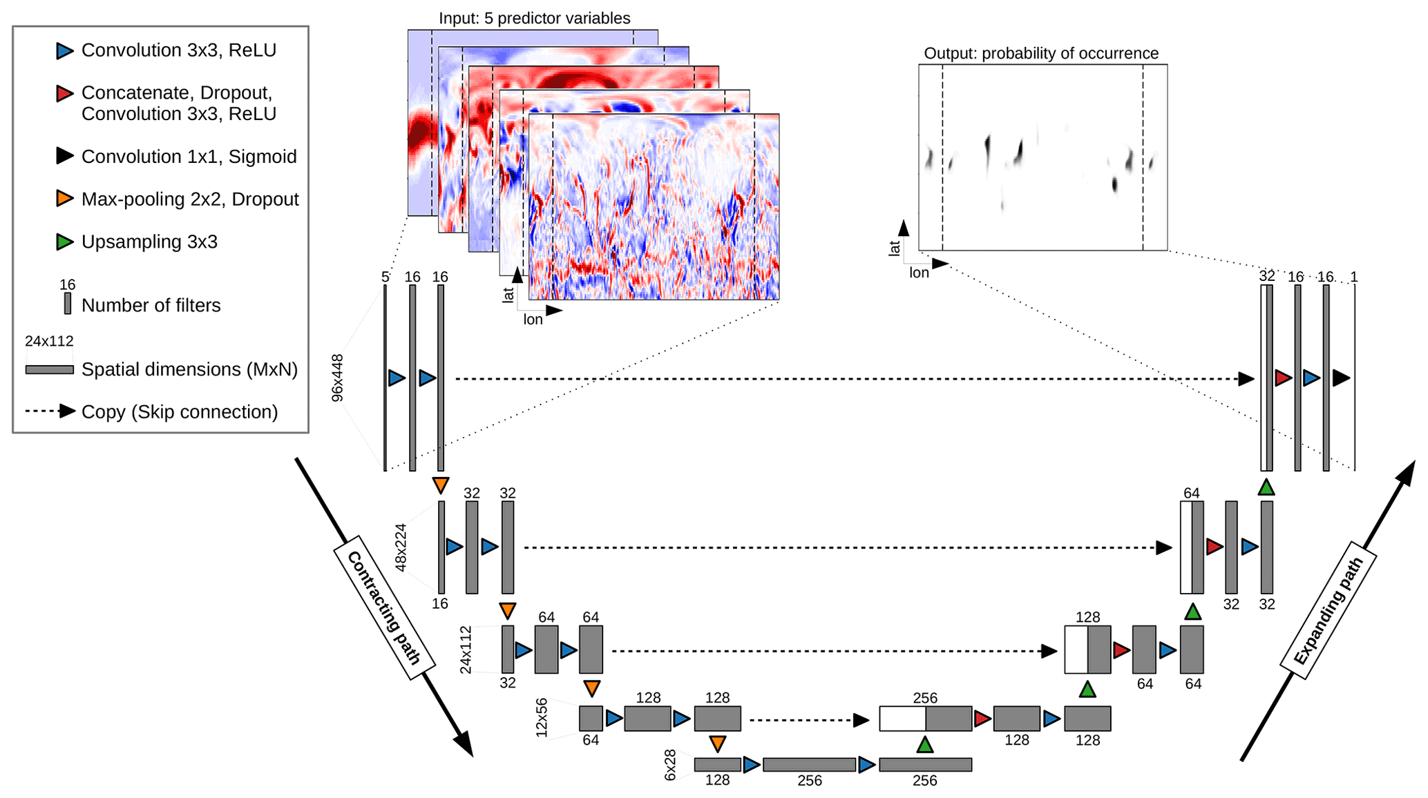
Figure 1The architecture of the UNet, which follows an encoder–decoder structure with a contracting path and an expanding path. Both paths consist of four blocks each with three layers. A final 1×1 convolutional layer reduces the number of feature maps from 16 to 1. See main text for detailed explanations.
3.1 Input map
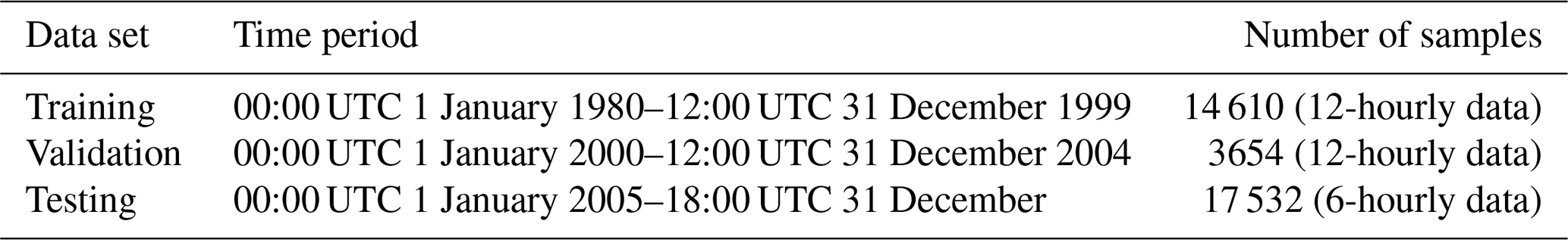
In a first step, the data introduced in Sect. 2 are split into training, validation, and testing data sets. An essential requirement is that the training, validation, and testing data sets are statistically independent. A random sampling from the entire time period to create the three subsets would likely lead to highly correlated data sets. For example, a sample from 00:00 UTC on one day could fall into the training set and a sample from 12:00 UTC on the same day into the testing set. The 12 h time interval between the two samples would be considerably shorter than the synoptic timescale on which WCBs evolve. To avoid statistical dependence, we split the data into the three subsets as shown in Table 2. The training data, which comprise the period 1 January 1980 to 31 December 1999, are used to train the CNN models. Validation data are a comparably small subset of 5 years that allow the comparison of models with different settings on unseen data and identification of the best-performing model. The testing data, which comprise the period 1 January 2005 to 31 December 2016, are used to evaluate the best-performing models on unseen data (Sect. 3). Though predictors and predictands are available at 00:00, 06:00, 12:00, and 18:00 UTC, we train and validate the CNN models with 12-hourly data (00:00, 12:00 UTC) for computational reasons. The computationally less expensive testing of the models is performed on 6-hourly data (00:00, 06:00, 12:00, 18:00 UTC).
Table 2Temporal data coverage of training, validation, and testing data for the CNN models.
Each training sample consists of input maps and an output map. The variable M is the number of rows (latitudes), N is the number of columns (longitudes), and P is the number of channels (number of predictor variables; P=5). The CNN models of this study contain at least four so-called max-pooling layers (see Sect. 3.2), each downsampling a map two times. Therefore, M and N have to be a multiple of 2n+1 (Ayzel et al., 2020), where n is the number of max-pooling layers. With horizontal grid spacing M would be 91 for the entire Northern Hemisphere and thus not a multiple of 2n+1. Accordingly, we decided to select data from 6∘ S to 89∘ N (M=96) in the latitudinal direction. The North Pole at 90∘ N is excluded due to infinite gradients when computing some of the predictors in Table 1 via finite differences. To account for the circular nature of the data in the longitudinal direction at the international dateline, input padding is performed (Shi et al., 2015; Schubert et al., 2019): we pad 44 grid points east and west of the dateline, which increases N from 360 to 448. As a result, the computing time needed for the model training increases. Still, it improves the results since without input padding the modeled probabilities would exhibit discontinuities along the dateline.
Prior to input padding each of the five predictor variables is normalized for each training sample to
where xi,j is the original value, denotes the area-weighted mean, and σ is the area-weighted standard deviation. The reasoning behind the normalization is to prevent predictors with large values from causing large weight updates in the CNN during training (Sect. 3.4).
3.2 Contracting path
The default setting in this work is a contracting path with four blocks, each of which contains two convolutional layers (blue triangles in Fig. 1). These layers transform the input maps into so-called feature maps using convolutional filters. The convolutional filters are three-dimensional tensors of learnable weights with a certain spatial kernel size (kernel size 3×3 in this study) and the third dimension equal to that of the input map. The filters convolve through the input maps grid point by grid point with stride 1 in this study and perform a convolution defined as (e.g., Lagerquist et al., 2019)
where is the kth feature map in the ith layer, denotes the jth feature map in the (i−1)th layer, is the convolutional filter, J is the number of feature maps in the (i−1)th layer, is the bias for the kth feature map in the ith layer, and f is the activation function. We use the rectified linear unit (ReLU; Nair and Hinton, 2010) as an activation function in order to add nonlinearities to the convolutional layer output. This nonlinearity is required since otherwise the CNNs would only learn linear relationships. The third layer of each block is a 2×2 max-pooling layer (orange triangles in Fig. 1), which slides over each feature map with stride 1 and takes the maximum of four numbers in the filter region of 2×2 grid points. Accordingly, the feature maps are downsampled by a factor of 2. For example, the original size of the input map is 96×448, and after the first block, which contains one max-pooling layer, it is reduced to 48×224. The process of convolution and max pooling is repeated for each block. With each block, the number of filters doubles so that the models are able to detect the meaningful features of the input maps effectively. Each max-pooling layer is followed by a dropout regularization layer, which aims to prevent overfitting (Srivastava et al., 2014). During dropout regularization, input units are randomly set to 0 with a pre-defined dropout fraction at each step during training time. Here, we decided to test the sensitivity of the results to the dropout fraction by varying it in the range from 0.0 to 0.3 at intervals of 0.05 (see Sect. 3.5). Dropout regularization is not used during validation and testing. Further, we apply batch normalization (Ioffe and Szegedy, 2015)1 after each dropout layer, which effectively reduces overfitting in CNNs and reduces the number of training steps.
3.3 Expanding path
In line with the contracting path the expanding path consists of four blocks, each of which contains three layers. The first layer is a transposed convolutional layer and serves the purpose of up-sampling the feature maps from low to higher resolution. The kernel sizes are set to 3×3, and the stride is two. The up-sampling is followed by the second layer, which first concatenates the feature maps from the contracting path to the expanding path (so-called skip connections), second applies a dropout function, and third includes a convolutional layer with a kernel size of 3×3 and stride 1. By including skip connections (black dashed arrows in Fig. 1), high-resolution information from the contracting path can be used in order to reconstruct high-resolution feature maps in the expanding path. The third layer is a further convolutional layer with the same kernel size and stride as in the previous layer. After each expanding block the number of filters halves in contrast to the contracting blocks. The spatial dimensions double with each expanding block so that the size of the feature map is 96×448 after four expansions, which is the same size as the original input map.
The final output is generated with a convolutional layer (kernel size 1×1; stride 1; black triangle in Fig. 1), which reduces the number of feature maps from 16 to 1. In contrast to all previous convolutional layers, the activation function is a sigmoid function yielding values between 0 and 1 so that the output can be interpreted as a conditional probability.
3.4 Model training
Random initialization of the convolutional filters ensures that they all have different weights and biases . Accordingly, the different filters detect different features on the input map. The weights and biases of all convolutional filters are updated during iterative training via the Adam optimization algorithm (Kingma and Ba, 2015). The purpose is to minimize a loss function for classification, which in this study is the binary cross-entropy loss. It is defined as
and is commonly used for binary classification tasks. N is the number of scalar values in the model output, denotes the probability that the ith example is a WCB, and yi is the corresponding target value (WCB yes or no).
The weights and biases are optimized using at most 20 training iterations (called epochs in the context of machine learning) with batch sizes ranging from 8 to 64. The initial learning rate of the Adam optimizer is set to and is reduced by a factor of 0.1 when the binary cross-entropy does not improve over the course of five consecutive iterations. Further, the training stops early if the binary cross-entropy does not improve in 10 consecutive iterations.
3.5 Model setting optimization
In this section, we evaluate the performance of different models setups for the validation period (1 January 2000 to 31 December 2004) in order to find the optimal setting of parameters. A particular focus is on the hyperparameters dropout fraction and batch size. Further, we evaluate the effect of omitting the WCB climatology as a predictor (4block_16filters in Fig. 2), adding an additional fifth block to the UNet CNN (5block_WCBCLIM_16filters in Fig. 2), and increasing the number of initial filters from 16 to 32 (4block_WCBCLIM_32filters in Fig. 2). We try all 102 possible combinations of the parameters listed in Table 3.
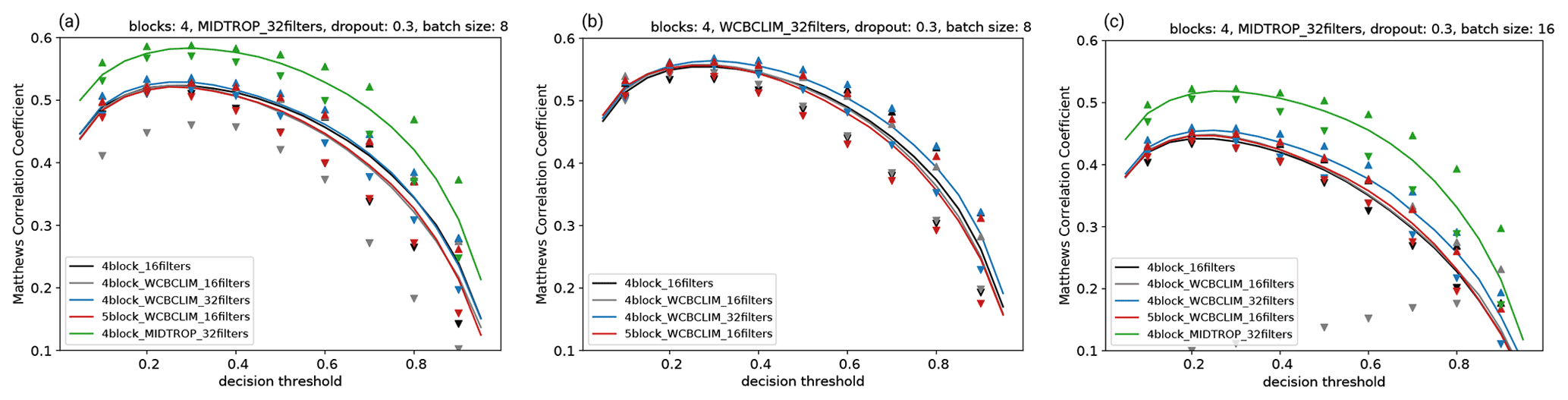
Figure 2MCC values for (a) WCB inflow, (b) WCB ascent, and (c) WCB outflow as a function of the decision thresholds for different parameter settings described in Sect. 3.5 and listed in Table 3. MCC values are averaged over grid points for which the 30 d running mean climatological WCB frequency reaches at least 1 %. Lines are medians over all experiments with varied dropout fraction and batch size. Down- and up-pointing triangles denote their minimum and maximum values, respectively. The model configuration reaching the highest MCC is given in the title of each panel.
Table 3Parameters that are used to find the best parameter setup for the standard models.
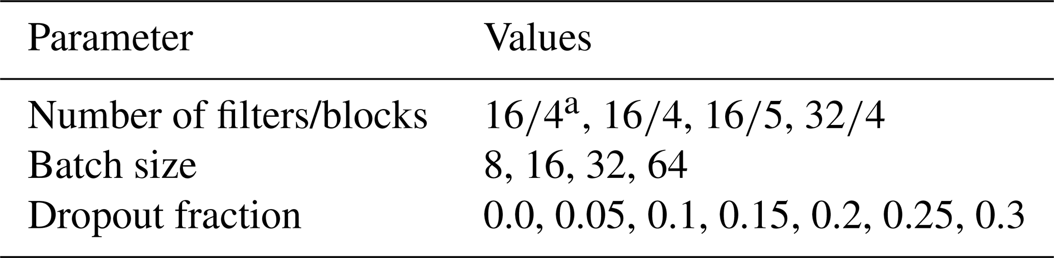
a In these experiments the WCB climatology of WCB inflow, ascent, and outflow is omitted as a predictor.
In order to find the optimal configuration, we assess the model performance on the entire set of validation data in terms of the Matthews correlation coefficient (Matthews, 1975, MCC). The MCC is a balanced skill metric for binary verification tasks, even if the two classes are imbalanced as is the case with WCBs which occur at some grid points only in 1 % of the cases. The MCC is defined as
with TP, TN, FP, and FN being the number of true positives, true negatives, false positives, and false negatives. The MCC values range from –1 (total disagreement between prediction and observations) to 1 (perfect prediction). An MCC value of 0 indicates a random prediction. As the calculation of the MCC requires deterministic predictions (WCB yes or no), we evaluate it for the validation data at different decision thresholds ranging from 0.05 to 0.95 at intervals of 0.05 above which the modeled probabilities are set to 1. The MCC is calculated grid-point-wise but only at grid points for which the 30 d running mean climatological WCB occurrence frequency based on the period 1 January 1980 to 31 December 2016 reaches at least 1 %. It should be noted that MCC values obtained from this grid-point-wise evaluation are rather on the conservative side since slight offsets between predictions and observations are unduly punished. Accordingly, object-based or neighborhood-based evaluations (e.g., Lagerquist et al., 2019; Silverman et al., 2021) would yield even higher MCC values.
To begin with, we only focus on the standard models and their median MCC values (black, gray, blue, and red lines Fig. 2) as a function of the decision thresholds. For all three WCB stages, WCB inflow (Fig. 2a), ascent (Fig. 2b), and outflow (Fig. 2c), the median MCC values for the different number of filters and blocks exhibit sensitivities of less than 5 %. Even when not using the running mean WCB climatology as a fifth predictor, the median MCC does not decrease markedly (black line in Fig. 2). Larger sensitivities are found concerning the dropout fraction and batch size, especially for decision thresholds larger than 0.5 as indicated by the wide range between the minimum (down-pointing triangles) and maximum (up-pointing triangles) MCC values. However, for the range of decision thresholds between 0.2 and 0.4 that yield the overall highest MCC, the range between the minimum and maximum MCC is less than 5 % of the corresponding median MCC. For all three WCB stages, a standard model consisting of four layers and 32 filters yields the highest MCC (blue up-pointing triangles in Fig. 2). Of all standard models, the highest MCC values are reached for WCB ascent.
This result inspired us to test an additional CNN model configuration for the WCB stages of inflow and outflow: as outlined in the Introduction, the inflow of a WCB precedes the ascent stage and the outflow lags the ascent stage. Accordingly, we decided to account for this relationship by replacing the fifth predictor of the standard models for inflow and outflow (30 d running mean WCB climatology) with the conditional WCB ascent probability predicted by the optimal WCB ascent model at a certain time lag. Here we decided for a time lag of 24 h because the model is to be applied to forecasts of the sub-seasonal to seasonal prediction project database (Vitart et al., 2017), which are available 24-hourly. Thus, the fifth predictor is the conditional probability of WCB ascent 24 h later (earlier) than the corresponding WCB inflow (outflow) time. These models are referred to as time-lag models. Indeed, the median MCC values for WCB inflow and outflow improve by almost 20 % when taking the conditional probability of WCB ascent as a fifth predictor (4block_MIDTROP_32filters; green line in Fig. 2a and c). The highest median MCC for WCB inflow even exceeds that for WCB ascent. As for the standard models the variations related to the parameter settings of dropout fraction and batch size are comparably small. The overall highest MCC values are reached with dropout fractions of 0.3 and batch sizes of 8 for inflow and ascent as well as 16 for outflow. It should be noted that the differences in terms of the MCC between the best and second-best model are marginal. With a slightly different training period, slightly different dropout fractions and batch sizes may be considered optimal. Accordingly, the parameter testing is by no means comprehensive, and additional parameter testing may yield better results. For the remainder of this study, we use the time-lag models with four blocks, 32 filters, a dropout fraction of 0.3 and batch sizes of 8 for inflow and ascent as well as 16 for outflow (see headings in Fig. 2a–c).
The models are evaluated in terms of their reliability, biases, and skill for the entire testing period (1 January 2005 to 31 December 2016), though results are only shown for DJF and JJA, i.e., the seasons with the highest and lowest climatological WCB occurrence frequency, respectively (Madonna et al., 2014). Further, we compare the reliability and skill of the CNN models to the logistic regression models of Quinting and Grams (2021b) introduced in Sect. 1.
4.1 Reliability
The average agreement between the observed WCB frequencies and the modeled WCB probabilities for DJF and JJA is shown as reliability diagrams in Fig. 3. For this purpose, the predicted probabilities are divided into 19 regular bins from 0.05 to 0.95 and plotted against the observed frequencies in these bins. Following Bröcker and Smith (2007), the observed frequencies are not plotted versus the arithmetic center of each bin, but against the average of the forecast values in each bin. Further, we perform consistency resampling (Bröcker and Smith, 2007), which provides information on the uncertainties of the reliability arising due to varying bin means as well as varying bin populations. The resampling step is repeated 1000 times, yielding 1000 surrogate observed relative frequencies for each bin. The range between the 5 % and 95 % quantiles is displayed as vertical consistency bars in Fig. 3. In the case of a perfect model the observed frequencies would fall within the consistency bars. A model overestimates (underestimates) the observed WCB frequency when the model's curve lies below (above) the range of the consistency bars.
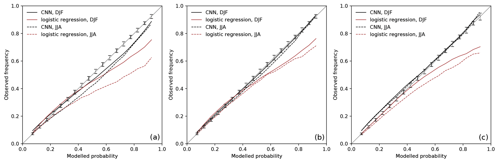
Figure 3Reliability diagrams for (a) inflow, (b) ascent, and (c) outflow during DJF (solid lines) and JJA (dashed lines). The black curves represent the reliability of the CNN models, and the red curves represent the reliability of the logistic regression models (Quinting and Grams, 2021b). Modeled probabilities (x axis) and observed frequencies (y axis) are binned into 19 bins based on the modeled probabilities. The range between the 5 % and 95 % quantiles of the consistency resampling is given for DJF and JJA by solid and dashed vertical bars, respectively.
For DJF and JJA, the CNN models tend to slightly overestimate the observed WCB inflow frequency at modeled probabilities greater than 0.35 and 0.15, respectively (Fig. 3a). The overestimation is more pronounced in JJA. The CNN models clearly outperform the logistic regression models for modeled probabilities greater than 0.3 in JJA and greater than 0.5 in DJF. As for the logistic regression models in Quinting and Grams (2021b), the CNN models perform best for WCB ascent (Fig. 3b). For DJF and JJA, the reliability curve is nearly entirely within the range of the consistency bars except for a slight overestimation during JJA for modeled probabilities between 0.45 and 0.8. For WCB outflow, the reliability curves lie within the range of the consistency bars during DJF and JJA for modeled probabilities greater than 0.5. For modeled probabilities of less than 0.5 the reliability curve is slightly outside the 95 % quantile of the consistency bars (Fig. 3c). This indicates that the CNN model underestimates the observed frequencies. Still, the CNN model is more reliable than the logistic regression models, which overestimate the observed frequencies considerably for modeled probabilities greater 0.5 and 0.7 during JJA and DJF, respectively.
4.2 Model bias
The evaluation of the bias and skill (see Sect. 4.3) of the CNN models requires categorical and/or deterministic predictions (WCB yes or no). Therefore, the probabilistic CNN model predictions need to be categorized by applying a decision threshold above which a modeled probability is considered to be WCB inflow, WCB ascent, or WCB outflow. Following Quinting and Grams (2021b), the decision threshold is chosen to be grid-point-dependent and to minimize the climatological bias of the models at each grid point. Here, bias is defined as the difference between the trajectory-based climatological WCB frequency and the CNN-based climatological WCB frequency in the testing period (1 January 2005–31 December 2016). The decision thresholds are assessed as follows.
-
For each day of the year we compute a 90 d running mean Lagrangian WCB climatology. Although the assessment of reliability, bias, and skill is performed for the testing period (1 January 2005–31 December 2016), the climatological WCB frequency used to define the decision thresholds is based on the entire period (1 January 1980–31 December 2016) in order to account for possible long-term variations of the WCB occurrence frequency. Further, if we had only used the testing period for the definition of the climatological WCB frequency neighboring grid points may have been categorized differently (WCB yes or no) despite exhibiting equal conditional probabilities. Taking the entire period for the calculation of the climatology yields spatially smoother thresholds and thus avoids such inconsistencies.
-
We then loop over a decision threshold at intervals of 0.01 above which the conditional probability predicted by the CNN is set to 1.
-
For each day of the year and for each value of the decision threshold we compute a 90 d running mean climatology based on the CNN model predictions.
-
For each day of the year and each grid point, we determine the optimal pWCB that produces the lowest bias between the trajectory-based and CNN-based WCB climatology.
The purpose of calculating a decision threshold pWCB for each day of the year is to account for seasonal variations of the modeled probabilities. For WCB inflow, ascent, and outflow the decision threshold is highest in winter and lowest in summer (not shown).
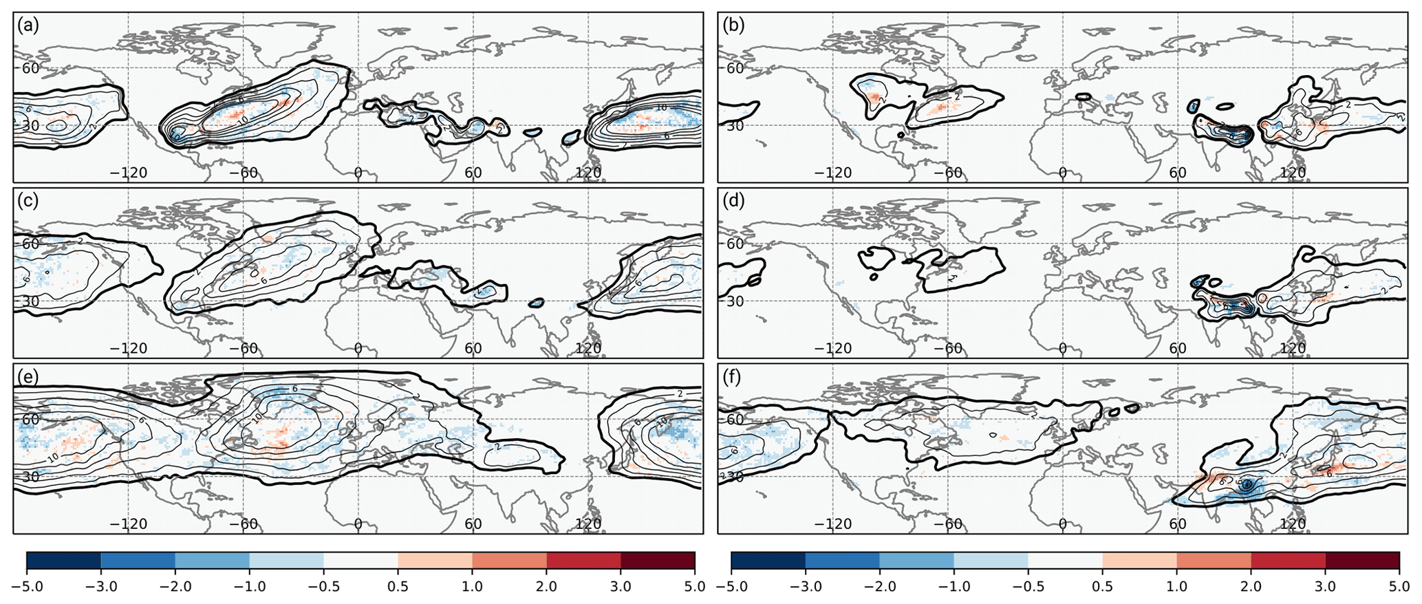
Figure 4Climatological occurrence frequency bias for WCB (a, b) inflow, (c, d) ascent, and (e, f) outflow (shading is absolute frequency bias in percent) of the CNN models compared to the trajectory-based climatology (thick black contour at 1 %; thin black contours every 2 %). Panels (a, c, e) are for DJF in the period 1 December 2005 to 29 February 2016, and panels (b, d, f) are for JJA in the period 1 June 2005 to 31 August 2015.
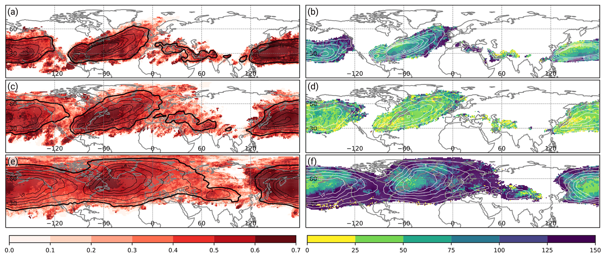
Figure 5Matthews correlation coefficient of the CNN models during DJF for (a) WCB inflow, (c) WCB ascent, and (e) WCB outflow (shading). Relative difference in terms of the Matthews correlation coefficient between the CNN model and the logistic regression models in Quinting and Grams (2021b) for (b) WCB inflow, (d) WCB ascent, and (f) WCB outflow (shading in %). Relative difference is only shown at grid points for which the climatological Lagrangian WCB frequency reaches at least 1 % since the logistic regression models are not available at grid points with a lower climatological frequency. Contours denote the climatological Lagrangian WCB frequency (thick black contour at 1 %; thin black and white contours every 2 %) for the respective WCB stage. All panels are shown for DJF in the period 1 December 2005 to 29 February 2016.
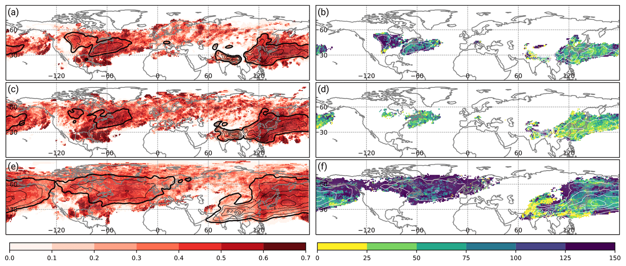
Figure 6As in Fig. 5 except that all panels are shown for JJA in the period 1 June 2005 to 31 August 2015.
In the following, we analyze to what degree the climatological occurrence frequency of WCB inflow, ascent, and outflow based on gridded trajectories is represented by the CNN-based approach (Fig. 4) in the testing period. By design of the decision threshold above which a predicted probability is considered to be a WCB, the observed frequency and that of the regression model coincide well. During DJF, the model bias for WCB inflow, ascent, and outflow is less than 2 % at all grid points. Also in JJA, the biases are of similar magnitude except for the region related to the Asian monsoon over northern India (Fig. 4b, d, and f). Here, the frequency bias reaches up to 3 %.
4.3 Model skill
The skill of the CNN models is quantified in terms of the MCC during the testing period. For WCB inflow and during DJF, the models' skill is highest in the climatologically most frequent inflow regions over the western to central North Pacific and the western to central North Atlantic (Fig. 5a). Especially in regions where the climatological WCB inflow frequency exceeds 10 %, the MCC reaches values of 0.6 to 0.7. Compared to the logistic regression model the MCC improves in most regions by at least 50 % (Fig. 5b), which corresponds to an absolute improvement of the MCC by 0.3. The improvements are most pronounced in regions of comparably low climatological WCB inflow frequency, indicating that the CNN models also perform well on data with limited availability of training samples.
The MCC values for WCB ascent are of similar magnitude (Fig. 5c). Again, the highest MCC values greater than 0.6 are collocated with the climatological occurrence frequency maxima over the Atlantic and western to central North Pacific. Even in regions where the climatological occurrence frequency is on the order of 1 %, the MCC exhibits values of at least 0.5. The improvement of the MCC compared to the logistic regression model is positive everywhere (Fig. 5d), but smaller than for WCB inflow and outflow. Still, the mean MCC for WCB ascent is the second highest of the three WCB stages (see Fig. 2).
The MCC for WCB outflow is lower than for WCB inflow and WCB ascent. The highest MCC values of 0.6 to 0.7 are found over eastern North America, the Labrador Sea, and the western to central North Pacific (Fig. 5e). Thus, as for WCB inflow and ascent, the regions of highest model skill are collocated with regions exhibiting the highest climatological WCB outflow frequency. The relative improvement compared to the logistic regression models is particularly pronounced in the regions with the climatologically lowest WCB outflow occurrence frequency. The absolute value of the MCC exceeds that of the regression models by more than 0.25, which corresponds in some locations to a relative increase of more than 125 % (Fig. 5f).
During boreal summer (JJA) the frequency of WCB inflow, ascent, and outflow is considerably lower than during DJF. WCB inflow occurs most frequently over central North America, the western North Atlantic, and East Asia to the central North Pacific (Fig. 6a). A further maximum north of India is related to the Asian monsoon. On average the MCC for WCB inflow tends to be lower during JJA than during DJF. Still, in regions with a climatological frequency of more than 2 %, the MCC reaches values of 0.4 to 0.6, which corresponds to a relative improvement of 50 % over the western North Pacific and more than 125 % over central North America compared to the logistic regression models.
The MCC values for WCB inflow and WCB ascent are of similar magnitude. Although the climatological frequency is only about 2 % in the storm-track regions of the North Atlantic and the North Pacific, the MCC still exceeds 0.5 in these areas (Fig. 6c). The absolute value of MCC improves by more than 0.15 compared to the regression models in most regions, which corresponds to a relative increase of 25 %–50 % (Fig. 6d).
Also in JJA, the MCC is lower for WCB outflow than during DJF. In regions where the WCB outflow occurrence frequency exceeds 2 %, the MCC mostly exceeds values of 0.4 (Fig. 6e). However, in regions of climatologically low WCB outflow occurrence frequency the MCC is on the order of 0.2 to 0.3, which is most likely related to the comparably small training sample size in those areas. Especially in high latitudes over the North Pacific and over the entire North Atlantic, the MCC improves by more than 100 % compared to the logistic regression models at most grid points.
Prior to the logistic regression model development, Quinting and Grams (2021b) identified the best predictors for the three stages of WCB inflow, ascent, and outflow via stepwise forward selection. Here, we take the opposite approach and use the fully developed CNN models to address the question of which of the predictors used for the time-lag models have the largest impact on the predictions and are thus most characteristic for each of the WCB stages. Following Breiman (2001) and Gagne et al. (2019), we choose a model-agnostic interpretation method known as permutation feature importance, which treats the model as a black box and only operates on the inputs and outputs. Permutation feature importance ranks predictors based on how randomizing their values affects the models' skill. More specifically, we take the models' MCC skill of Sect. 4.3 as a reference and compare it to the MCC skill of predictions; predictor P1 (Table 1) for each WCB stage is sampled at a random date from the testing period. The remaining four predictors are sampled at the exact same date. This process is repeated for predictors P2 to P5 so that the skill of five different predictions in terms of the MCC can be compared. The larger the decrease in MCC, the higher the importance of the corresponding predictor. Though the normalization of the input data should reduce the effect of seasonal variations, we still take the random dates from a window of 30 d around the actual date.
According to the permutation feature importance, the most important predictor variable for WCB inflow during DJF is the conditional probability of WCB ascent 24 h later (referred to as MIDTROP in Fig. 7a and b). The average skill decrease in terms of the MCC is twice as high as the decrease when perturbing the 1000 hPa moisture flux convergence and 850 hPa meridional moisture flux (Fig. 7a). It is only at the edges of the climatologically most active WCB inflow regions that moisture flux convergence and the meridional moisture flux are identified as most important predictors. Also during JJA, the conditional probability of WCB ascent with a time lag of 24 h is the most important predictor for WCB inflow (Fig. 8a and b). It is followed by the 1000 hPa moisture flux convergence and the 850 hPa meridional moisture flux. The 700 hPa thickness advection and the 500 hPa moist PV are of minor importance in both seasons. That the conditional probability of WCB ascent with a time lag of 24 h is the most important predictor for WCB inflow is in line with the original trajectory-based definition wherein a temporal relation between the two stages is given by definition. The comparably high importance of variables related to moisture flux is in line with the findings for the logistic regression models but also with the general concept of WCB inflow, which is typically characterized by strong moisture flux convergence and bands of high water vapor transport (Wernli and Davies, 1997; Dacre et al., 2019).
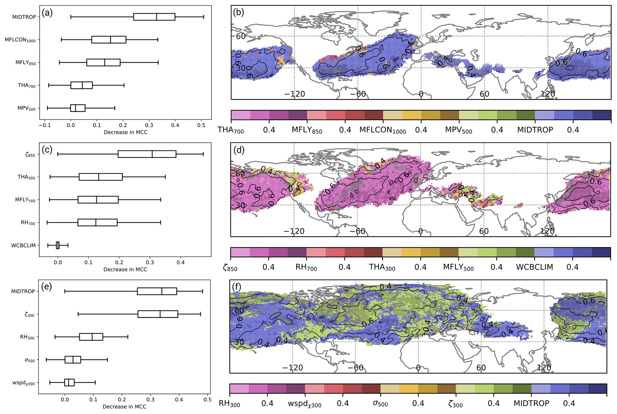
Figure 7Feature importance scores in terms of the reduction in MCC for (a, b) WCB inflow, (c, d) WCB ascent, and (e, f) WCB outflow. Box-and-whisker plots in (a, c, e) show the median (vertical line), interquartile range (boxes), and the 5th and 95th percentiles of the decrease in MCC over all grid points at which the climatological occurrence frequency reaches at least 1 %. Shading in (b, d, f) shows the decrease in MCC when perturbing the most important predictor. The darker the shading (at intervals of 0.2), the greater the decrease in the MCC. Black contours indicate the MCC of the reference prediction at intervals of 0.1.
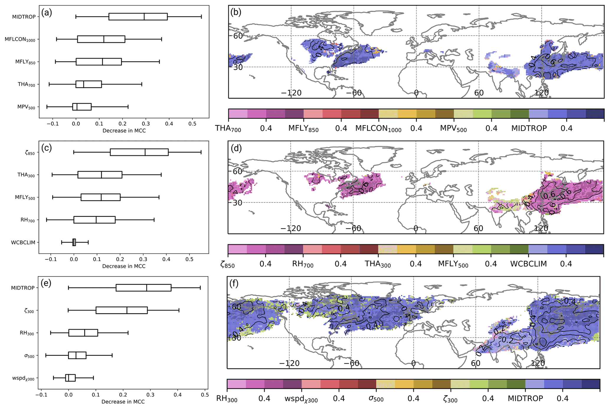
Figure 8As in Fig. 7 except that all panels are shown for JJA in the period 1 June 2005 to 31 August 2015.
For WCB ascent, a permutation of the 850 hPa relative vorticity leads to the strongest decrease in model skill (Figs. 7c and 8c). In particular over the western North Pacific and the western North Atlantic the MCC decreases to values near 0 when perturbing the relative vorticity field (Figs. 7d and 8d). These findings are the same for DJF and JJA. During WCB ascent, relative vorticity is redistributed via stretching so that cyclonic vorticity increases in the lower troposphere (Binder et al., 2016). Thus, the overall importance of relative vorticity for WCB ascent is in line with physical considerations. The decrease in the MCC for WCB ascent due to permutations of the 300 hPa thickness advection, 850 hPa meridional moisture flux, and 700 hPa relative humidity exhibits similar values. The seemingly least important predictor is the climatological WCB occurrence frequency with a median decrease in MCC close to zero. However, one should keep in mind that the random dates are taken only from a window of 30 d around the actual date. By doing so, the importance of the climatological WCB occurrence frequency for predicting the seasonal cycle of WCB activity is likely underestimated.
The almost equally most important predictor variables for WCB outflow during DJF are the conditional probability of WCB ascent 24 h before and the 300 hPa relative vorticity (Fig. 7e and f). Interestingly, over the North Pacific the WCB ascent predictor is most important at nearly all grid points, while over the North Atlantic the 300 hPa relative vorticity is the most important predictor at about half of all grid points. During the summer months, the 300 hPa relative vorticity becomes less important (Fig. 8e). At nearly all grid points the conditional probability of WCB ascent is the most important predictor (Fig. 8f). It is only in regions with the climatologically lowest WCB frequency that the 300 hPa relative vorticity and the 300 hPa irrotational wind speed are still the most important predictors. The importance of the conditional probability of WCB ascent with a time lag of −24 h coincides with the trajectory-based WCB identification for which this relation is given by definition. The importance of the 300 hPa relative vorticity is most likely related to the fact that WCB outflow is most often found in upper-tropospheric anticyclonic ridges (e.g., Pomroy and Thorpe, 2000; Grams et al., 2011).
In this study, we introduce a UNet CNN that identifies WCB footprints from Eulerian fields, which are available from NWP and climate models. For each of the WCB stages of WCB inflow, ascent, and outflow a separate CNN model is developed. The CNN-based framework is trained for the Northern Hemisphere on 20 years of gridded trajectory-based WCB data derived from ERA-Interim using the same physical predictors as in Quinting and Grams (2021b). The climatological occurrence frequency of WCB inflow, ascent, and outflow serves as an additional predictor for the respective WCB stage. With these predictors, the UNet standard models consisting of four layers with an initial set of 32 filters yield the best results for WCB ascent. Sensitivities to the hyperparameters dropout fraction and batch size are found to be small. Given that the CNN model performs best for the WCB ascent stage, we make use of the temporal succession of the three WCB stages to predict WCB inflow and outflow. For WCB inflow and outflow, the fifth predictor in the standard models is replaced by the conditional probability of WCB ascent predicted with the CNN model at a time lag of 24 and −24 h, respectively. With this approach, the improvement of the CNN models for inflow and outflow is considerably larger than any variations of the hyperparameters so that we consider these models to be optimal. The importance of the time-lagged conditional probability of WCB ascent as a predictor for WCB inflow and outflow is confirmed by the model-agnostic permutation feature importance. Further important predictors related to moisture flux for WCB inflow or relative vorticity for WCB ascent and outflow are in line with previous trajectory-based studies and highlight the capability of the CNNs to identify WCBs based on dynamical features that are in agreement with the general concept of WCBs. The CNN models for WCB inflow, ascent, and outflow are evaluated for an unseen testing period covering 1 January 2005 to 31 December 2016. For all three WCB stages, the models' reliability is within the 10 % interval around the reliability of a perfect model. The models reach a similar reliability during boreal summer and winter. Most notably, the models outperform the logistic regression models of Quinting and Grams (2021b), which tend to overestimate the frequency of WCBs at any of the three stages. The modeled probabilities are converted to dichotomous predictions by determining a decision threshold such that the climatological bias of the models is minimized. For all three stages, the models reach the highest skill in terms of the Matthews correlation coefficient in the midlatitude storm-track regions, i.e., in regions where the climatological occurrence frequency of WCBs is highest. Compared to the logistic regression models, the relative skill improvement reaches up to 100 %, which is due to both the addition of spatial information via convolution and the nonlinear activation functions, which account for nonlinear relationships between the predictors and predictands.
Despite their overall success the deep learning models still come with certain limitations. Compared to the trajectory approach, the CNNs do not conserve the number of individual trajectories such that the inflow footprints can in principle represent a larger number of trajectories than the outflow. CNNs that are trained to output the actual number of trajectories instead of conditional probabilities could be one way forward. Physical constraints have been introduced to deep learning approaches (e.g., Kashinath et al., 2021) such that mass conservation between the inflow and outflow could be aimed for in a future version of the models. Further, the sensitivity of the models' skill to climate change has not been evaluated yet. With the advent of the ERA5 reanalysis and its availability for a 70-year period such sensitivity tests would be worthwhile to pursue.
Our study demonstrates that deep learning allows transferring a sophisticated diagnostic, which relies on high-resolution data and considerable computing time, into a reliable and almost unbiased tool, which works on coarser data with significantly less computing time. This opens promising pathways regarding how to use machine learning for process-oriented studies on big data sets such as ensemble NWP reforecasts or climate model projections that have so far been inaccessible due to diagnostic constraints. For example, the CNN-based WCB models can be used to investigate the representation of the climatological frequency of WCBs in these data sets but also of the link of WCB activity and midlatitude synoptic systems such as cyclones or blocking. The feature importance opens ways to pin down biases in the WCB frequency to biases in the predictor variables. Moreover, the high skill in instantaneous WCB identification allows using the WCB diagnostic as an additional inexpensive feature identification tool in case studies. Examples of such applications are discussed in Part 2 of this study. It includes an analysis of the climatological link between WCBs, cyclones, and blocking, an analysis of WCB frequency biases in ECMWF's operational ensemble forecasts, and examples showing the versatile applicability of the CNN-based models to modeling systems other than ECMWF.
Ultimately, we do not argue that deep learning approaches should or can replace sophisticated diagnostic tools. Rather, they should be used in concert with the latter by first establishing a fundamental understanding of physical processes based on an in-depth investigation of data sets with high spatiotemporal resolution. In a second step, a companion deep learning diagnostic such as presented in this study facilitates testing the representation of such processes in larger data sets from NWP and climate models.
The exact version of the time-lag models, the decision thresholds, the 30 d running mean trajectory-based WCB climatology, and code to process the input data for the models are provided via the repository at https://git.scc.kit.edu/nk2448/wcbmetric_v2.git (Quinting, 2022) and archived on Zenodo (https://doi.org/10.5281/zenodo.5154980, Quinting and Grams, 2021a). ERA-Interim data are freely available at https://apps.ecmwf.int/datasets/data/interim-full-daily (ECMWF, 2022). The LAGRANTO documentation and information on how to access the source code are provided in Sprenger and Wernli (2015).
JFQ developed the models and conducted the model evaluation. CMG provided the initial idea. JFQ and CMG jointly discussed and interpreted the results and prepared the paper.
The contact author has declared that neither they nor their co-author has any competing interests.
Publisher's note: Copernicus Publications remains neutral with regard to jurisdictional claims in published maps and institutional affiliations.
This work was funded by the Helmholtz Association as part of the Young Investigator Group “Sub-seasonal Predictability: Understanding the Role of Diabatic Outflow” (SPREADOUT, grant VH-NG-1243). The research was partially embedded in the subprojects A8 and B8 of the Transregional Collaborative Research Center SFB/TRR 165 “Waves to Weather” (https://www.wavestoweather.de/, last access: 13 January 2022) funded by the German Research Foundation (DFG). Sincerest thanks to the Atmospheric Dynamics group at ETH Zurich, in particular to Michael Sprenger and Heini Wernli for sharing the trajectory-based WCB data. We are grateful to Sebastian Lerch at KIT for an inspiring workshop that motivated the implementation of the CNN and to the Large-Scale Dynamics and Predictability group at KIT for helpful discussions. Further, we would like to thank two anonymous reviewers for the valuable comments that helped to improve the presentation of our results. ECMWF, Deutscher Wetterdient, and MeteoSwiss are acknowledged for granting access to the ERA-Interim data set.
This research has been supported by the Helmholtz-Gemeinschaft (grant no. VH-NG-1243).
The article processing charges for this open-access publication were covered by the Karlsruhe Institute of Technology (KIT).
This paper was edited by Travis O'Brien and reviewed by two anonymous referees.
Ayzel, G., Scheffer, T., and Heistermann, M.: RainNet v1.0: a convolutional neural network for radar-based precipitation nowcasting, Geosci. Model Dev., 13, 2631–2644, https://doi.org/10.5194/gmd-13-2631-2020, 2020. a, b
Baumgart, M., Riemer, M., Wirth, V., Teubler, F., and Lang, S. T.: Potential vorticity dynamics of Forecast errors: A quantitative case study, Mon. Weather Rev., 146, 1405–1425, https://doi.org/10.1175/MWR-D-17-0196.1, 2018. a
Berman, J. D. and Torn, R. D.: The impact of initial condition and warm conveyor belt forecast uncertainty on variability in the downstream waveguide in an ECWMF case study, Mon. Weather Rev., 147, 4071–4089, https://doi.org/10.1175/MWR-D-18-0333.1, 2019. a
Binder, H., Boettcher, M., Joos, H., and Wernli, H.: The role of warm conveyor belts for the intensification of extratropical cyclones in Northern Hemisphere winter, J. Atmos. Sci., 73, 3997–4020, https://doi.org/10.1175/JAS-D-15-0302.1, 2016. a, b
Bosart, L. F., Moore, B. J., Cordeira, J. M., Archambault, H. M., Bosart, L. F., Moore, B. J., Cordeira, J. M., and Archambault, H. M.: Interactions of North Pacific tropical, midlatitude, and polar disturbances resulting in linked extreme weather events over North America in October 2007, Mon. Weather Rev., 145, 1245–1273, https://doi.org/10.1175/MWR-D-16-0230.1, 2017. a
Bowman, K. P., Lin, J. C., Stohl, A., Draxler, R., Konopka, P., Andrews, A., and Brunner, D.: Input data requirements for Lagrangian trajectory models, B. Am. Meteorol. Soc., 94, 1051–1058, https://doi.org/10.1175/BAMS-D-12-00076.1, 2013. a
Breiman, L.: Random forests, Mach. Learn., 45, 5–32, https://doi.org/10.1023/A:1010933404324, 2001. a
Browning, K. A. and Roberts, N. M.: Structure of a frontal cyclone, Q. J. Roy. Meteor. Soc., 120, 1535–1557, https://doi.org/10.1002/qj.49712052006, 1994. a
Bröcker, J. and Smith, L. A.: Increasing the Reliability of Reliability Diagrams, Weather Forecast., 22, 651–661, https://doi.org/10.1175/WAF993.1, https://journals.ametsoc.org/view/journals/wefo/22/3/waf993_1.xml, 2007. a, b
Carlson, T. N.: Airflow through midlatitude cyclones and the comma cloud pattern., Mon. Weather Rev., 108, 1498–1509, https://doi.org/10.1175/1520-0493(1980)108<1498:ATMCAT>2.0.CO;2, 1980. a
Dacre, H. F., Martínez-Alvarado, O., and Mbengue, C. O.: Linking atmospheric rivers and warm conveyor belt airflows, J. Hydrometeorol., 20, 1183–1196, https://doi.org/10.1175/JHM-D-18-0175.1, 2019. a
Dee, D. P., Uppala, S. M., Simmons, A. J., Berrisford, P., Poli, P., Kobayashi, S., Andrae, U., Balmaseda, M. A., Balsamo, G., Bauer, P., Bechtold, P., Beljaars, A. C., van de Berg, L., Bidlot, J., Bormann, N., Delsol, C., Dragani, R., Fuentes, M., Geer, A. J., Haimberger, L., Healy, S. B., Hersbach, H., Hólm, E. V., Isaksen, L., Kållberg, P., Köhler, M., Matricardi, M., Mcnally, A. P., Monge-Sanz, B. M., Morcrette, J. J., Park, B. K., Peubey, C., de Rosnay, P., Tavolato, C., Thépaut, J. N., and Vitart, F.: The ERA-Interim reanalysis: Configuration and performance of the data assimilation system, Q. J. Roy. Meteor. Soc., 137, 553–597, https://doi.org/10.1002/qj.828, 2011. a
Eckhardt, S., Stohl, A., Wernli, H., James, P., Forster, C., and Spichtinger, N.: A 15 year climatology of warm conveyor belts, J. Climate, 17, 218–237, https://doi.org/10.1175/1520-0442(2004)017<0218:AYCOWC>2.0.CO;2, 2004. a, b
ECMWF: ERA Interim, Daily, ECMWF [data set], available at: https://apps.ecmwf.int/datasets/data/interim-full-daily/levtype=sfc/, last access:13 January 2022. a
Eyring, V., Bony, S., Meehl, G. A., Senior, C. A., Stevens, B., Stouffer, R. J., and Taylor, K. E.: Overview of the Coupled Model Intercomparison Project Phase 6 (CMIP6) experimental design and organization, Geosci. Model Dev., 9, 1937–1958, https://doi.org/10.5194/gmd-9-1937-2016, 2016. a
Fukushima, K. and Miyake, S.: Neocognitron: A new algorithm for pattern recognition tolerant of deformations and shifts in position, Pattern Recogn., 15, 455–469, https://doi.org/10.1016/0031-3203(82)90024-3, 1982. a
Gagne, D. J., Haupt, S. E., Nychka, D. W., and Thompson, G.: Interpretable deep learning for spatial analysis of severe hailstorms, Mon. Weather Rev., 147, 2827–2845, https://doi.org/10.1175/MWR-D-18-0316.1, 2019. a
Grams, C. M., Wernli, H., Böttcher, M., Čampa, J., Corsmeier, U., Jones, S. C., Keller, J. H., Lenz, C. J., and Wiegand, L.: The key role of diabatic processes in modifying the upper-tropospheric wave guide: A North Atlantic case-study, Q. J. Roy. Meteor. Soc., 137, 2174–2193, https://doi.org/10.1002/qj.891, 2011. a, b, c
Grams, C. M., Magnusson, L., and Madonna, E.: An atmospheric dynamics perspective on the amplification and propagation of forecast error in numerical weather prediction models: A case study, Q. J. Roy. Meteor. Soc., 144, 2577–2591, https://doi.org/10.1002/qj.3353, 2018. a
Hamill, T. M. and Kiladis, G. N.: Skill of the MJO and Northern Hemisphere blocking in GEFS medium-range reforecasts, Mon. Weather Rev., 142, 868–885, https://doi.org/10.1175/MWR-D-13-00199.1, 2014. a
Harrold, T. W.: Mechanisms influencing the distribution of precipitation within baroclinic disturbances, Q. J. Roy. Meteor. Soc., 99, 232–251, https://doi.org/10.1002/qj.49709942003, 1973. a
Ioffe, S. and Szegedy, C.: Batch normalization: Accelerating deep network training by reducing internal covariate shift, in: ICML'15: Proceedings of the 32nd International Conference on International Conference on Machine Learning, Lille, France, 6–11 July 2015, JMLR.org, 37, 448–456, available at: http://proceedings.mlr.press/v37/ioffe15.pdf (last access: 13 January 2022), 2015. a
Kashinath, K., Mustafa, M., Albert, A., Wu, J. L., Jiang, C., Esmaeilzadeh, S., Azizzadenesheli, K., Wang, R., Chattopadhyay, A., Singh, A., Manepalli, A., Chirila, D., Yu, R., Walters, R., White, B., Xiao, H., Tchelepi, H. A., Marcus, P., Anandkumar, A., Hassanzadeh, P., and Prabhat: Physics-informed machine learning: Case studies for weather and climate modelling, Philos. T. Roy. Soc. A, 379, 20200093, https://doi.org/10.1098/rsta.2020.0093, 2021. a
Kingma, D. P. and Ba, J. L.: Adam: A method for stochastic optimization, 3rd International Conference on Learning Representations, in: ICLR 2015 – 3rd International Conference on Learning Representations, San Diego, CA, USA, 7–9 May 2015, Conference Track Proceedings, 1–15, available at: https://arxiv.org/pdf/1412.6980.pdf (last access: 13 January 2022), 2015. a
Kumler-Bonfanti, C., Stewart, J., Hall, D., and Govett, M.: Tropical and extratropical cyclone detection using deep learning, J. Appl. Meteorol. Clim., 59, 1971–1985, https://doi.org/10.1175/JAMC-D-20-0117.1, 2020. a
Lagerquist, R., McGovern, A. M., and Gagne, D. J.: Deep learning for spatially explicit prediction of synoptic-scale fronts, Weather Forecast., 34, 1137–1160, https://doi.org/10.1175/WAF-D-18-0183.1, 2019. a, b, c
Lamberson, W. S., Torn, R. D., Bosart, L. F., and Magnusson, L.: Diagnosis of the source and evolution of medium-range forecast errors for extratropical Cyclone Joachim, Weather Forecast., 31, 1197–1214, https://doi.org/10.1175/WAF-D-16-0026.1, 2016. a
Lebedev, V., Ivashkin, V., Rudenko, I., Ganshin, A., Molchanov, A., Ovcharenko, S., Grokhovetskiy, R., Bushmarinov, I., and Solomentsev, D.: Precipitation nowcasting with satellite imagery, Proceedings of the ACM SIGKDD International Conference on Knowledge Discovery and Data Mining, Association for Computing Machinery, New York, NY, USA, 2680–2688, https://doi.org/10.1145/3292500.3330762, 2019. a
Lu, C., Kong, Y., and Guan, Z.: A mask R-CNN model for reidentifying extratropical cyclones based on quasi-supervised thought, Sci. Rep., 10, 1–9, https://doi.org/10.1038/s41598-020-71831-z, 2020. a
Maddison, J. W., Gray, S. L., Martínez-Alvarado, O., and Williams, K. D.: Upstream cyclone influence on the predictability of block onsets over the Euro-Atlantic region, Mon. Weather Rev., 147, 1277–1296, https://doi.org/10.1175/MWR-D-18-0226.1, 2019. a
Madonna, E., Wernli, H., Joos, H., and Martius, O.: Warm conveyor belts in the ERA-Interim Dataset (1979–2010). Part I: Climatology and potential vorticity evolution, J. Climate, 27, 3–26, https://doi.org/10.1175/JCLI-D-12-00720.1, 2014. a, b, c, d
Martínez-Alvarado, O., Madonna, E., Gray, S. L., and Joos, H.: A route to systematic error in forecasts of Rossby waves, Q. J. Roy. Meteor. Soc., 142, 196–210, https://doi.org/10.1002/qj.2645, 2016. a, b
Matsuoka, D., Nakano, M., Sugiyama, D., and Uchida, S.: Deep learning approach for detecting tropical cyclones and their precursors in the simulation by a cloud-resolving global nonhydrostatic atmospheric model, Progress in Earth and Planetary Science, 5, 1–16, https://doi.org/10.1186/s40645-018-0245-y, 2018. a
Matthews, B. W.: Comparison of the predicted and observed secondary structure of T4 phage lysozyme, BBA-Protein Struct., 405, 442–451, https://doi.org/10.1016/0005-2795(75)90109-9, 1975. a
Muszynski, G., Kashinath, K., Kurlin, V., Wehner, M., and Prabhat: Topological data analysis and machine learning for recognizing atmospheric river patterns in large climate datasets, Geosci. Model Dev., 12, 613–628, https://doi.org/10.5194/gmd-12-613-2019, 2019. a
Nair, V. and Hinton, T. J.: Rectified Linear Units Improve Restricted Boltzmann Machines, in: ICML'10: Proceedings of the 27th International Conference on International Conference on Machine Learning, Haifa, Israel, 21–24 June 2010, Omnipress, Madison, WI, USA, 807–814, available at: https://icml.cc/Conferences/2010/papers/432.pdf (last access: 13 January 2022), 2010. a
Pegion, K., Kirtman, B. P., Becker, E., Collins, D. C., Lajoie, E., Burgman, R., Bell, R., Delsole, T., Min, D., Zhu, Y., Li, W., Sinsky, E., Guan, H., Gottschalck, J., Joseph Metzger, E., Barton, N. P., Achuthavarier, D., Marshak, J., Koster, R. D., Lin, H., Gagnon, N., Bell, M., Tippett, M. K., Robertson, A. W., Sun, S., Benjamin, S. G., Green, B. W., Bleck, R., and Kim, H.: The subseasonal experiment (SUBX), B. Am. Meteorol. Soc., 100, 2043–2060, https://doi.org/10.1175/BAMS-D-18-0270.1, 2019. a
Pomroy, H. R. and Thorpe, A. J.: The evolution and dynamical role of reduced upper-tropospheric potential vorticity in intensive observing period one of FASTEX, Mon. Weather Rev., 128, 1817–1834, https://doi.org/10.1175/1520-0493(2000)128<1817:TEADRO>2.0.CO;2, 2000. a, b
Prabhat, Kashinath, K., Mudigonda, M., Kim, S., Kapp-Schwoerer, L., Graubner, A., Karaismailoglu, E., von Kleist, L., Kurth, T., Greiner, A., Mahesh, A., Yang, K., Lewis, C., Chen, J., Lou, A., Chandran, S., Toms, B., Chapman, W., Dagon, K., Shields, C. A., O'Brien, T., Wehner, M., and Collins, W.: ClimateNet: an expert-labeled open dataset and deep learning architecture for enabling high-precision analyses of extreme weather, Geosci. Model Dev., 14, 107–124, https://doi.org/10.5194/gmd-14-107-2021, 2021. a, b
Quinting, J.: EuLerian Identification of ascending AirStreams - ELIAS 2.0: GitLab [data set], available at: https://git.scc.kit.edu/nk2448/wcbmetric_v2, last access: 13 January 2022. a
Quinting, J. and Grams, C. M: EuLerian Identification of ascending AirStreams (ELIAS 2.0) in Numerical Weather Prediction and Climate Models, Zenodo [code], https://doi.org/10.5281/zenodo.5154980, 2021a. a
Quinting, J. F. and Grams, C. M.: Toward a Systematic Evaluation of Warm Conveyor Belts in Numerical Weather Prediction and Climate Models. Part I: Predictor Selection and Logistic Regression Model, J. Atmos. Sci., 78, 1465–1485, https://doi.org/10.1175/JAS-D-20-0139.1, 2021b. a, b, c, d, e, f, g, h, i, j, k, l, m
Quinting, J. F., Grams, C. M., Oertel, A., and Pickl, M.: EuLerian Identification of ascending AirStreams (ELIAS 2.0) in numerical weather prediction and climate models – Part 2: Model application to different datasets, Geosci. Model Dev., 15, 731–744, https://doi.org/10.5194/gmd-15-731-2022, 2022. a
Rodwell, M. J., Richardson, D. S., Parsons, D. B., and Wernli, H.: Flow-dependent reliability: A path to more skillful ensemble forecasts, B. Am. Meteorol. Soc., 99, 1015–1026, https://doi.org/10.1175/BAMS-D-17-0027.1, 2018. a
Ronneberger, O., Fischer, P., and Brox, T.: U-Net: Convolutional Networks for Biomedical Image Segmentation, in: Medical Image Computing and Computer-Assisted Intervention – MICCAI 2015, edited by: Navab, N., Hornegger, J., Wells, W. M., and Frangi, A. F., Springer International Publishing, Cham, pp. 234–241, 2015. a, b
Sánchez, C., Methven, J., Gray, S., and Cullen, M.: Linking Rapid Forecast Error Growth to Diabatic Processes, Q. J. Roy. Meteor. Soc., 146, 3548–3569, https://doi.org/10.1002/qj.3861, 2020. a
Schäfler, A., Boettcher, M., Grams, C. M., Rautenhaus, M., Sodemann, H., and Wernli, H.: Planning aircraft measurements within a warm conveyor belt, Weather, 69, 161–166, https://doi.org/10.1002/wea.2245, 2014. a
Schubert, S., Neubert, P., Poschmann, J., and Pretzel, P.: Circular convolutional neural networks for panoramic images and laser data, in: 2019 IEEE Intelligent Vehicles Symposium (IV), Paris, France, 9–12 June 2019, IEEE, 653–660, https://doi.org/10.1109/IVS.2019.8813862, 2019. a
Shi, B., Bai, S., Zhou, Z., and Bai, X.: DeepPano: Deep Panoramic Representation for 3-D Shape Recognition, IEEE Signal Proc. Let., 22, 2339–2343, https://doi.org/10.1109/LSP.2015.2480802, 2015. a
Silverman, V., Nahum, S., and Raveh-Rubin, S.: Predicting origins of coherent air mass trajectories using a neural network–the case of dry intrusions, Meteorol. Appl., 28, 1–18, https://doi.org/10.1002/met.1986, 2021. a, b
Sprenger, M. and Wernli, H.: The LAGRANTO Lagrangian analysis tool – version 2.0, Geosci. Model Dev., 8, 2569–2586, https://doi.org/10.5194/gmd-8-2569-2015, 2015. a
Sprenger, M., Fragkoulidis, G., Binder, H., Croci-Maspoli, M., Graf, P., Grams, C. M., Knippertz, P., Madonna, E., Schemm, S., Škerlak, B., and Wernli, H.: Global climatologies of Eulerian and Lagrangian flow features based on ERA-Interim, B. Am. Meteorol. Soc., 98, 1739–1748, https://doi.org/10.1175/BAMS-D-15-00299.1, 2017. a
Srivastava, N., Hinton, G. E., Krizhevsky, A., Sutskever, I., and Salakhutdinov, R. R.: Dropout: A Simple Way to Prevent Neural Networks from Overfitting, J. Mach. Learn. Res., 15, 1929–1958, 2014. a
Stohl, A., Haimberger, L., Scheele, M. P., and Wernli, H.: An intercomparison of results from three trajectory models, Meteorol. Appl., 8, 127–135, https://doi.org/10.1017/S1350482701002018, 2001. a
Vitart, F., Ardilouze, C., Bonet, A., Brookshaw, A., Chen, M., Codorean, C., Déqué, M., Ferranti, L., Fucile, E., Fuentes, M., Hendon, H., Hodgson, J., Kang, H. S., Kumar, A., Lin, H., Liu, G., Liu, X., Malguzzi, P., Mallas, I., Manoussakis, M., Mastrangelo, D., MacLachlan, C., McLean, P., Minami, A., Mladek, R., Nakazawa, T., Najm, S., Nie, Y., Rixen, M., Robertson, A. W., Ruti, P., Sun, C., Takaya, Y., Tolstykh, M., Venuti, F., Waliser, D., Woolnough, S., Wu, T., Won, D. J., Xiao, H., Zaripov, R., and Zhang, L.: The subseasonal to seasonal (S2S) prediction project database, B. Am. Meteorol. Soc., 98, 163–173, https://doi.org/10.1175/BAMS-D-16-0017.1, 2017. a, b, c, d
Wandel, J., Quinting, J. F., and Grams, C. M.: Toward a Systematic Evaluation of Warm Conveyor Belts in Numerical Weather Prediction and Climate Models. Part II: Verification of Operational Reforecasts, J. Atmos. Sci., 78, 3965–3982, https://doi.org/10.1175/JAS-D-20-0385.1, 2021. a
Wernli, H.: A Lagrangian-based analysis of extratropical cyclones. II: A detailed case-study, Q. J. Roy. Meteor. Soc., 123, 1677–1706, https://doi.org/10.1256/smsqj.54210, 1997. a
Wernli, H. and Davies, H. C.: A Lagrangian-based analysis of extratropical cyclones. I: The method and some applications, Q. J. Roy. Meteor. Soc., 123, 467–489, https://doi.org/10.1256/smsqj.53810, 1997. a, b, c
Wernli, H. and Schwierz, C.: Surface cyclones in the ERA-40 dataset (1958–2001). Part I: Novel identification method and global climatology, J. Atmos. Sci., 63, 2486–2507, https://doi.org/10.1175/JAS3766.1, 2006. a
Weyn, J. A., Durran, D. R., and Caruana, R.: Improving Data-Driven Global Weather Prediction Using Deep Convolutional Neural Networks on a Cubed Sphere, J. Adv. Model. Earth Sy., 12, e2020MS002109, https://doi.org/10.1029/2020MS002109, 2020. a
During model training (Sect. 3.4), the training data set is divided into so-called batches. In brief, the batch size defines the number of training samples considered before updating the filter weights, and batch normalization describes the process of normalizing the input maps in one batch prior to proceeding with the training.
- Abstract
- Introduction
- Data
- UNet convolutional neural network
- Model evaluation
- Identifying the most relevant dynamical footprint of WCBs by interpreting feature importance in the CNN models
- Conclusions
- Code and data availability
- Author contributions
- Competing interests
- Disclaimer
- Acknowledgements
- Financial support
- Review statement
- References