OpenArray v1.0: a simple operator library for the decoupling  of ocean modeling and parallel computing

Huang, Xiaomeng; Huang, Xing; Wang, Dong; Wu, Qi; Li, Yi; Zhang, Shixun; Chen, Yuwen; Wang, Mingqing; Gao, Yuan; Tang, Qiang; Chen, Yue; Fang, Zheng; Song, Zhenya; Yang, Guangwen

doi:https://doi.org/10.5194/gmd-12-4729-2019

Articles | Volume 12, issue 11

https://doi.org/10.5194/gmd-12-4729-2019

Articles | Volume 12, issue 11

Development and technical paper

11 Nov 2019

Development and technical paper |

| 11 Nov 2019

OpenArray v1.0: a simple operator library for the decoupling of ocean modeling and parallel computing

Xiaomeng Huang, Xing Huang, Dong Wang, Qi Wu, Yi Li, Shixun Zhang, Yuwen Chen, Mingqing Wang, Yuan Gao, Qiang Tang, Yue Chen, Zheng Fang, Zhenya Song, and Guangwen Yang

Abstract

Rapidly evolving computational techniques are making a large gap between scientific aspiration and code implementation in climate modeling. In this work, we design a simple computing library to bridge the gap and decouple the work of ocean modeling from parallel computing. This library provides 12 basic operators that feature user-friendly interfaces, effective programming, and implicit parallelism. Several state-of-the-art computing techniques, including computing graph and just-in-time compiling, are employed to parallelize the seemingly serial code and speed up the ocean models. These operator interfaces are designed using native Fortran programming language to smooth the learning curve. We further implement a highly readable and efficient ocean model that contains only 1860 lines of code but achieves a 91 % parallel efficiency in strong scaling and 99 % parallel efficiency in weak scaling with 4096 Intel CPU cores. This ocean model also exhibits excellent scalability on the heterogeneous Sunway TaihuLight supercomputer. This work presents a promising alternative tool for the development of ocean models.

Download & links

Article (PDF, 4873 KB)

How to cite

How to cite.

Dates

Received: 01 Feb 2019 – Discussion started: 25 Feb 2019 – Revised: 19 Aug 2019 – Accepted: 26 Sep 2019 – Published: 11 Nov 2019

1 Introduction

Many earth system models have been developed in the past several decades to improve the predictive understanding of the earth system (Bonan and Doney, 2018; Collins et al., 2018; Taylor et al., 2012). These models are becoming increasingly complicated, and the amount of code has expanded from a few thousand lines to tens of thousands or even millions of lines. In terms of software engineering, an increase in code causes the models to be more difficult to develop and maintain.

The complexity of these models mainly originates from three aspects. First, more model components and physical processes have been embedded into the earth system models, leading to a 10-fold increase in the amount of code (e.g., Alexander and Easterbrook, 2015). Second, some heterogeneous and advanced computing platforms (e.g., Lawrence et al., 2018) have been widely used by the climate modeling community, resulting in a 5-fold increase in the amount of code (e.g., Xu et al., 2015). Last, most of the model programs need to be rewritten due to the continual development of novel numerical methods and meshes. The promotion of novel numerical methods and technologies produced in the fields of computational mathematics and computer science have been limited in climate science because of the extremely heavy burden caused by program rewriting and migration.

Over the next few decades, tremendous computing capacities will be accompanied by more heterogeneous architectures which are equipped with two or more kinds of cores or processing elements (Shan, 2006), thus making a much more sophisticated computing environment for climate modelers than ever before (National Research Council, 2012). Clearly, transiting the current earth system models to the next generation of computing environments will be highly challenging and disruptive. Overall, complex codes in earth system models combined with rapidly evolving computational techniques create a very large gap between scientific aspiration and code implementation in the climate modeling community.

To reduce the complexity of earth system models and bridge this gap, a universal and productive computing library is a promising solution. Through establishing an implicit parallel and platform-independent computing library, the complex models can be simplified and will no longer need explicit parallelism and transiting, thus effectively decoupling the development of ocean models from complicated parallel computing techniques and diverse heterogeneous computing platforms.

Many efforts have been made to address the complexity of parallel programming for numerical simulations, such as operator overloading, source-to-source translator, and domain-specific language (DSL). Operator overloading supports the customized data type and provides simple operators and function interfaces to implement the model algorithm. This technique is widely used because the implementation is straightforward and easy to understand (Corliss and Griewank, 1994; Walther et al., 2003). However, it is prone to work inefficiently because overloading execution induces numerous unnecessary intermediate variables, consuming valuable memory bandwidth resources. Using a source-to-source translator offers another solution. As indicated by the name, this method converts one language, which is usually strictly constrained by self-defined rules, to another (Bae et al., 2013; Lidman et al., 2012). It requires tremendous work to develop and maintain a robust source-to-source compiler. Furthermore, DSLs can provide high-level abstraction interfaces that use mathematical notations similar to those used by domain scientists so that they can write much more concise and more straightforward code. Some outstanding DSLs, such as ATMOL (van Engelen, 2001), ICON DSL (Torres et al., 2013), STELLA (Gysi et al., 2015), and ATLAS (Deconinck et al., 2017), are used by the numerical model community. Although they seem to be source-to-source techniques, DSLs are newly defined languages and produce executable programs instead of target languages. Therefore, the new syntax makes it difficult for the modelers to master the DSLs. In addition, most DSLs are not yet supported by robust compilers due to their relatively short history. Most of the source-to-source translators and DSLs still do not support the rapidly evolving heterogeneous computing platforms, such as the Chinese Sunway TaihuLight supercomputer which is based on the homegrown Sunway heterogeneous many-core processors and located at the National Supercomputing Center in Wuxi.

Other methods such as COARRAY Fortran and CPP templates provide alternative ways. Using COARRAY Fortran, a modeler has to control the reading and writing operation of each image (Mellor-Crummey et al., 2009). In a sense, one has to manipulate the images in parallel instead of writing serial code. In term of CPP templates, it is usually suitable for small amounts of code and difficult for debugging (Porkoláb et al., 2007).

Inspired by the philosophy of operator overloading, source-to-source translating and DSLs, we integrated the advantages of these three methods into a simple computing library which is called OpenArray. The main contributions of OpenArray are as follows:

Easy to use. The modelers can write simple operator expressions in Fortran to solve partial differential equations (PDEs). The entire program appears to be serial and the modelers do not need to know any parallel computing techniques. We summarized 12 basic generalized operators to support whole calculations in a particular class of ocean models which use the finite difference method and staggered grid.
High efficiency. We adopt some advanced techniques, including intermediate computation graphing, asynchronous communication, kernel fusion, loop optimization, and vectorization, to decrease the consumption of memory bandwidth and improve efficiency. Performance of the programs implemented by OpenArray is similar to the original but manually optimized parallel program.
Portability. Currently OpenArray supports both CPU and Sunway platforms. More platforms including GPU will be supported in the future. The complexity of cross-platform migration is moved from the models to OpenArray. The applications based on OpenArray can then be migrated seamlessly to the supported platforms.

Furthermore, we developed a numerical ocean model based on the Princeton Ocean Model (POM; Blumberg and Mellor, 1987) to test the capability and efficiency of OpenArray. The new model is called the Generalized Operator Model of the Ocean (GOMO). Because the parallel computing details are completely hidden, GOMO consists of only 1860 lines of Fortran code and is more easily understood and maintained than the original POM. Moreover, GOMO exhibits excellent scalability and portability on both central processing unit (CPU) and Sunway platforms.

The remainder of this paper is organized as follows. Section 2 introduces some concepts and presents the detailed mathematical descriptions of formulating the PDEs into operator expressions. Section 3 describes the detailed design and optimization techniques of OpenArray. The implementation of GOMO is described in Sect. 4. Section 5 evaluates the performances of OpenArray and GOMO. Finally, discussion and conclusion are given in Sects. 6 and 7, respectively.

2 Concepts of the array, operator, and abstract staggered grid

In this section, we introduce three important concepts in OpenArray: array, operator, and abstract staggered grid to illustrate the design of OpenArray.

2.1 Array

To achieve this simplicity, we designed a derived data type, Array, which inspired our project name, OpenArray. The new Array data type comprises a series of information, including a 3-dimensional (3-D) array to store data, a pointer to the computational grid, a Message Passing Interface (MPI) communicator, the size of the halo region, and other information about the data distribution. All the information is used to manipulate the Array as an object to simplify the parallel computing. In traditional ocean models, calculations for each grid point and the i, j, and k loops in the horizontal and vertical directions are unavoidable. The advantage of taking the Array as an object is the significant reduction in the number of loop operations in the models, making the code more intuitive and readable. When using the OpenArray library in a program, one can use type(Array) to declare new variables.

2.2 Operator

To illustrate the concept of an operator, we first take a 2-dimensional (2-D) continuous equation solving sea surface elevation as an example:

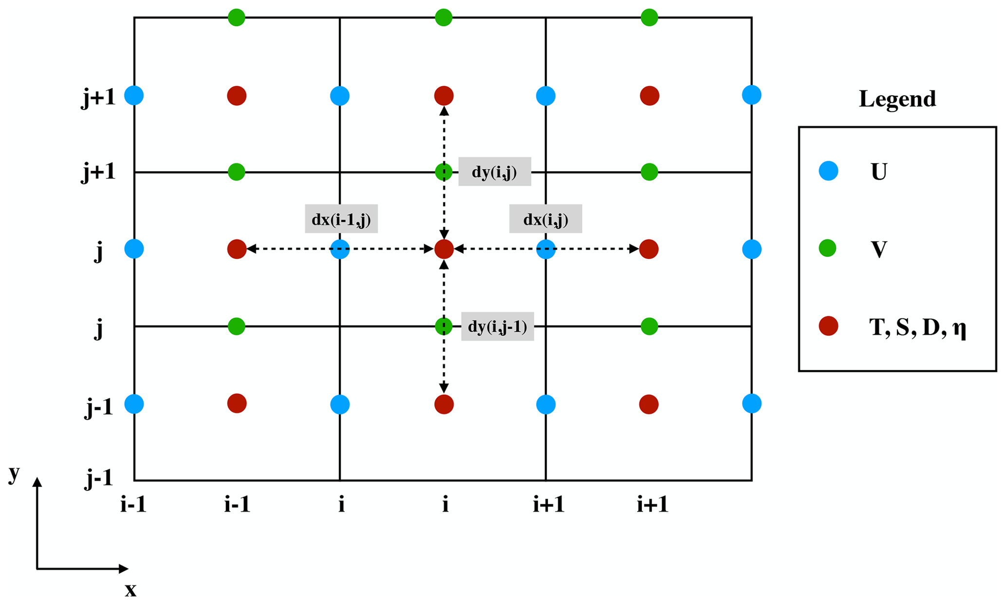
\begin{matrix} (1) & \frac{\partial η}{\partial t} + \frac{\partial D U}{\partial x} + \frac{\partial D V}{\partial y} = 0, \end{matrix}

where η is the surface elevation, U and V are the zonal and meridional velocities, and D is the depth of the fluid column. We choose the finite difference method and staggered Arakawa C grid scheme, which are adopted by most regional ocean models. In Arakawa C grid, D is calculated at the centers, U component is calculated at the left and right side of the variable D, and V component is calculated at the lower and upper side of the variable D (Fig. 1). Variables ( $D, U, V$ ) located at different positions own different sets of gird increments. Taking the term $\frac{\partial D U}{\partial x}$ as an example, we firstly apply linear interpolation to obtain the D^′s value at U point represented by tmpD. Through a backward difference to the product of tmpD and U, the discrete expression of $\frac{\partial D U}{\partial x}$ can be obtained.

\begin{matrix} (2) & \begin{aligned} tmpD (i + 1, j) = & 0.5 \cdot (D (i + 1, j) + D (i, j)) \\ \cdot U (i + 1, j), \end{aligned} \end{matrix}

and

\begin{matrix} (3) & \begin{aligned} \frac{\partial D U}{\partial x} = \frac{tmpD (i + 1, j) - tmpD (i, j)}{d x {(i, j)}^{*}} \\ = \frac{1}{2 \cdot d x (i, j)^{*}} \cdot ((D (i + 1, j) + D (i, j)) \cdot U (i + 1, j) \\ - (D (i, j) + D (i - 1, j)) \cdot U (i, j)), \end{aligned} \end{matrix}

where $d x {(i, j)}^{*} = 0.5 \cdot (d x (i, j) + d x (i - 1, j))$ .

https://www.geosci-model-dev.net/12/4729/2019/gmd-12-4729-2019-f01

Figure 1Arrangement of variables in the staggered Arakawa C grid.

Download

In this way, the above continuous equation can be discretized into the following form.

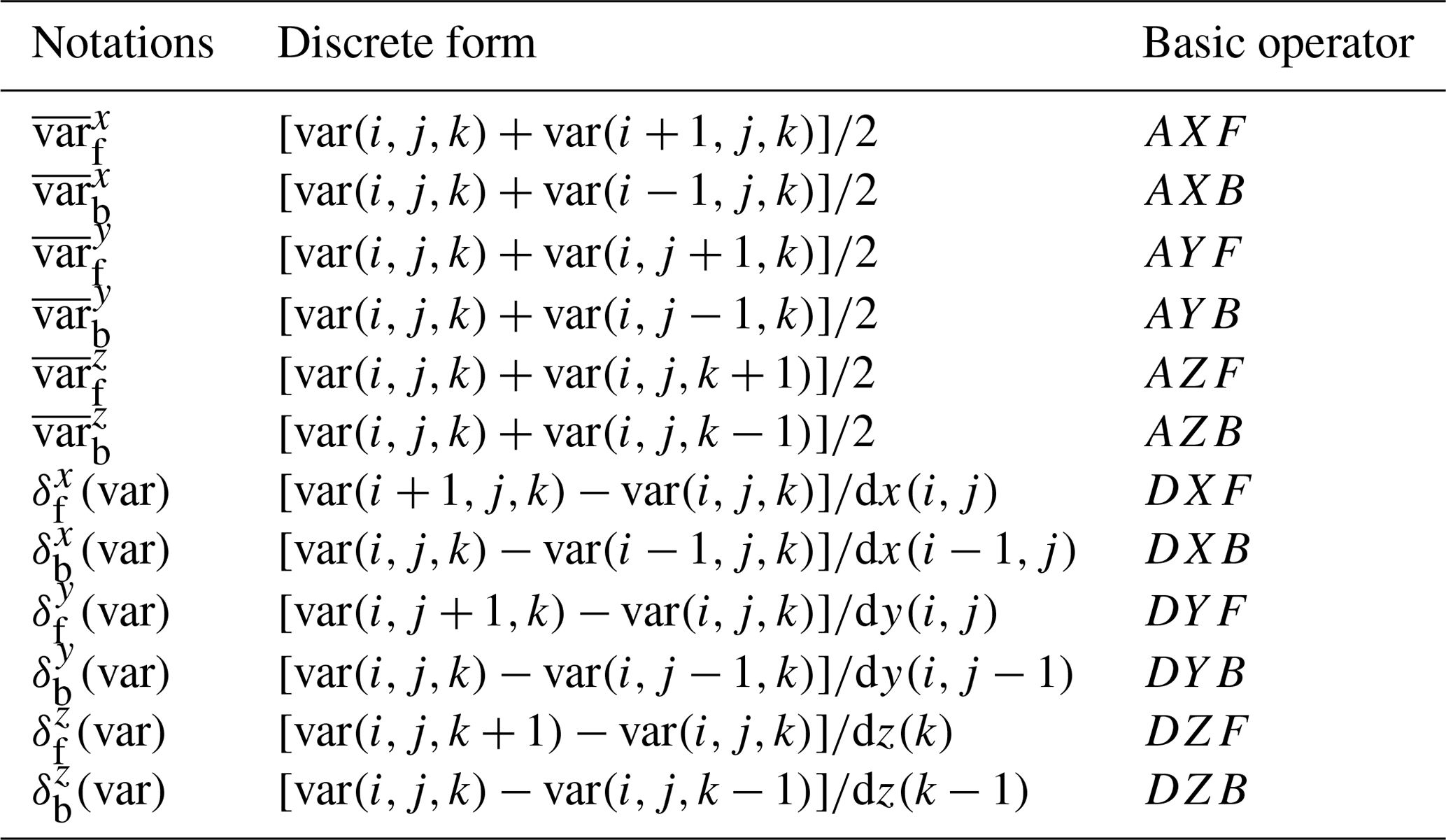
\begin{matrix} (4) & \begin{aligned} \frac{η_{t + 1} (i, j) - η_{t - 1} (i, j)}{2 \cdot d t} \\ + \frac{1}{2 \cdot d x {(i, j)}^{*}} \cdot ((D (i + 1, j) + D (i, j)) \cdot U (i + 1, j) \\ - (D (i, j) + D (i - 1, j)) \cdot U (i, j)) \\ + \frac{1}{2 \cdot d y {(i, j)}^{*}} ((D (i, j + 1) + D (i, j)) \cdot V (i, j + 1) \\ - (D (i, j) + D (i, j - 1)) \cdot V (i, j)) = 0, \end{aligned} \end{matrix}

where $d x {(i, j)}^{*} = 0.5 \cdot (d x (i, j) + d x (i - 1, j)), d y {(i, j)}^{*} = 0.5 \cdot (d y (i, j) + d y (i, j - 1))$ , and subscripts η_t+1 and η_t−1 denote the surface elevations at the (t+1) time step and (t−1) time step. To simplify the discrete form, we introduce some notation for the differentiation ( $δ_{f}^{x}$ , $δ_{b}^{y}$ ) and interpolation ( ${\overline{()}}_{f}^{x}$ , ${\overline{()}}_{b}^{y})$ . The δ and overbar symbols define the differential operator and average operator, respectively. The subscript x or y denotes that the operation acts in the x or y direction, and the superscript f or b denotes that the approximation operation is forward or backward.

Table 1 lists the detailed definitions of the 12 basic operators. The term var denotes a 3-D model variable. All 12 operators for the finite difference calculations are named using three letters in the form [A|D][ $X | Y | Z$ ][F|B]. The first letter contains two options, A or D, indicating an average or a differential operator. The second letter contains three options, X, Y, or Z, representing the direction of the operation. The last letter contains two options, F or B, representing forward or backward operation. The dx, dy, and dz are the distances between two adjacent grid points along the x, y, and z directions.

Table 1Definitions of the 12 basic operators.

Download Print Version | Download XLSX

Using the basic operators, Eq. (4) is expressed as

\begin{matrix} (5) & \frac{η_{t + 1} - η_{t - 1}}{2 \cdot d t} + δ_{f}^{x} ({\overline{D}}_{b}^{x} \cdot U) + δ_{f}^{y} ({\overline{D}}_{b}^{y} \cdot V) = 0 . \end{matrix}

Thus,

\begin{matrix} (6) & η_{t + 1} = η_{t - 1} - 2 \cdot d t \cdot (δ_{f}^{x} ({\overline{D}}_{b}^{x} \cdot U) + δ_{f}^{y} ({\overline{D}}_{b}^{y} \cdot V)) . \end{matrix}

Then, Eq. (6) can be easily translated into a line of code using operators (the bottom left part in Fig. 2). Compared with the pseudo-codes (the right part), the corresponding implementation by operators is more straightforward and more consistent with the equations.

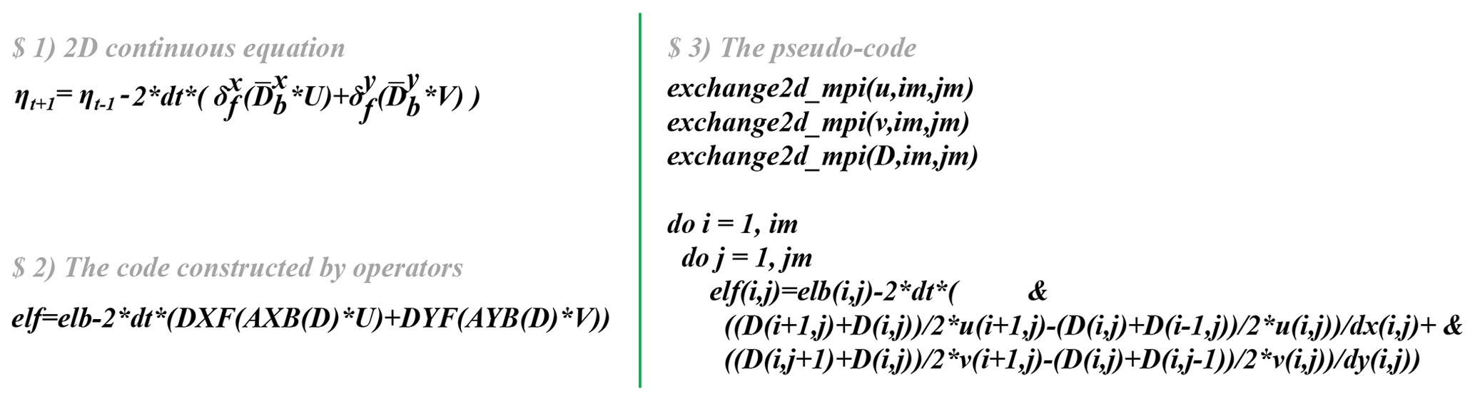
https://www.geosci-model-dev.net/12/4729/2019/gmd-12-4729-2019-f02

Figure 2Implementation of Eq. (6) by basic operators. The elf and elb variables are the surface elevations at times (t+1) and (t−1), respectively.

Download

Next, we will use the operators in shallow water equations, which are more complicated than those in the previous case. Assuming that the flow is in hydrostatic balance and that the density and viscosity coefficients are constant, and neglecting the molecular friction, the shallow water equations are

\begin{matrix} (7) & \frac{\partial η}{\partial t} + \frac{\partial D U}{\partial x} + \frac{\partial D V}{\partial y} = 0, \\ (8) & \begin{aligned} \frac{\partial D U}{\partial t} + \frac{\partial D U U}{\partial x} + \frac{\partial D V U}{\partial y} - f V D = - g D \frac{\partial η}{\partial x} \\ + μ D (\frac{\partial^{2} U}{\partial x^{2}} + \frac{\partial^{2} U}{\partial y^{2}}), \end{aligned} \end{matrix}

\begin{matrix} (9) & \begin{aligned} \frac{\partial D V}{\partial t} + \frac{\partial D U V}{\partial x} + \frac{\partial D V V}{\partial y} + f U D = - g D \frac{\partial η}{\partial y} \\ + μ D (\frac{\partial^{2} V}{\partial x^{2}} + \frac{\partial^{2} V}{\partial y^{2}}), \end{aligned} \end{matrix}

where f is the Coriolis parameter, g is the gravitational acceleration, and μ is the coefficient of kinematic viscosity. Using the Arakawa C grid and leapfrog time difference scheme, the discrete forms represented by operators are shown in Eqs. (10)–(12).

\begin{matrix} (10) & \frac{η_{t + 1} - η_{t - 1}}{2 \cdot d t} + δ_{f}^{x} ({\overline{D}}_{b}^{x} \cdot U) + δ_{f}^{y} ({\overline{D}}_{b}^{y} \cdot V) = 0, \\ (11) & \begin{aligned} \frac{D_{t + 1} U_{t + 1} - D_{t - 1} U_{t - 1}}{2 \cdot d t} + δ_{b}^{x} ({\overline{{\overline{D}}_{b}^{x} \cdot U}}_{f}^{x} \cdot {\overline{U}}_{f}^{x}) \\ + δ_{f}^{y} ({\overline{{\overline{D}}_{b}^{y} \cdot V}}_{b}^{x} \cdot {\overline{U}}_{b}^{y}) - {\overline{f {\overline{V}}_{f}^{y} \cdot D}}_{b}^{x} = - g \cdot {\overline{D}}_{b}^{x} \cdot δ_{b}^{x} (η) \\ + μ \cdot {\overline{D}}_{b}^{x} \cdot (δ_{b}^{x} (δ_{f}^{x} (U_{t - 1})) + δ_{f}^{y} (δ_{b}^{y} (U_{t - 1}))), \end{aligned} \\ (12) & \begin{aligned} \frac{D_{t + 1} V_{t + 1} - D_{t - 1} V_{t - 1}}{2 \cdot d t} + δ_{f}^{x} ({\overline{{\overline{D}}_{b}^{x} \cdot U}}_{b}^{y} \cdot {\overline{V}}_{b}^{x}) \\ + δ_{b}^{y} (\overline{{\overline{D}}_{b}^{y} \cdot V}_{f}^{y} \cdot {\overline{V}}_{f}^{y}) + {\overline{f {\overline{U}}_{f}^{x} \cdot D}}_{b}^{y} = - g \cdot {\overline{D}}_{b}^{y} \cdot δ_{b}^{y} (η) \\ + μ \cdot {\overline{D}}_{b}^{y} \cdot (δ_{f}^{x} (δ_{b}^{x} (V_{t - 1})) + δ_{b}^{y} (δ_{f}^{y} (V_{t - 1}))) . \end{aligned} \end{matrix}

As the shallow water equations are solved, spatial average and differential operations are called repeatedly. Implementing these operations is troublesome and thus it is favorable to abstract these common operations from PDEs and encapsulate them into user-friendly, platform-independent, and implicit parallel operators. As shown in Fig. 3, we require only three lines of code to solve the shallow water equations. This more realistic case suggests that even more complex PDEs can be constructed and solved by following this elegant approach.

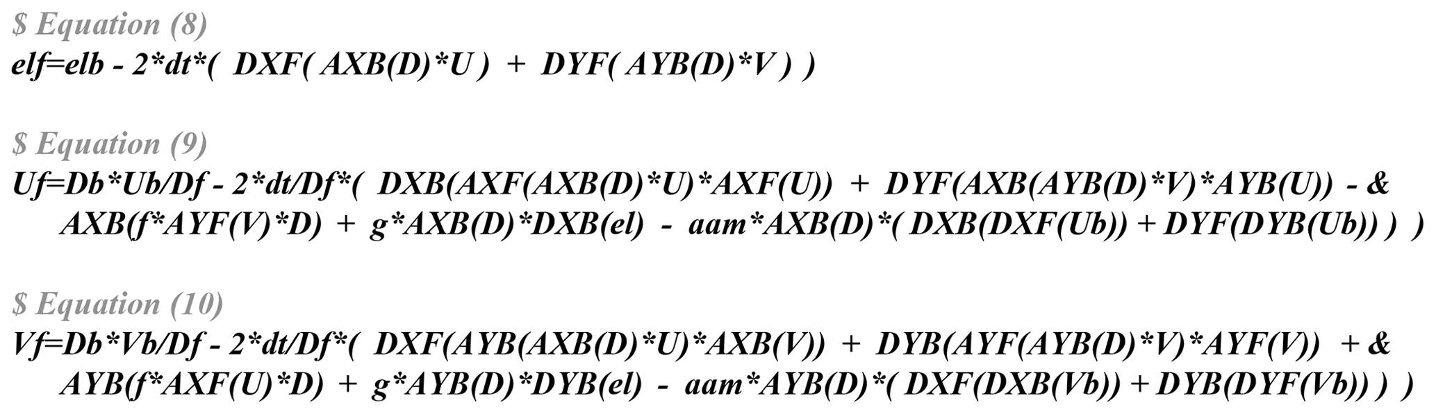
https://www.geosci-model-dev.net/12/4729/2019/gmd-12-4729-2019-f03

Figure 3Implementation of the shallow water equations by basic operators. elf, el, and elb denote sea surface elevations at times (t+1), t, and (t−1), respectively. Uf, U and Ub denote the zonal velocity at times (t+1), t, and (t−1), respectively. Vf, V, and Vb denote the meridional velocity at times (t+1), t, and (t−1), respectively. Variable aam denotes the viscosity coefficient.

Download

2.3 Abstract staggered grid

Most ocean models are implemented based on the staggered Arakawa grids (Arakawa and Lamb, 1981; Griffies et al., 2000). The variables in ocean models are allocated at different grid points. The calculations that use these variables are performed after several reasonable interpolations or differences. When we call the differential operations on a staggered grid, the difference value between adjacent points should be divided by the grid increment to obtain the final result. Setting the correct grid increment for modelers is troublesome work that is extremely prone to error, especially when the grid is nonuniform. Therefore, we propose an abstract staggered grid to support flexible switching of operator calculations among different staggered grids. When the grid information is provided at the initialization phase of OpenArray, a set of grid increments, including horizontal increments (dx(i,j), dy(i,j)), and vertical increment (dz(k)), will be combined with each corresponding physical variable through grid binding. Thus, the operators can implicitly set the correct grid increments for different Array variables, even if the grid is nonuniform.

As shown in Fig. 4, the cubes in the (a), (b), (c), and (d) panels are the minimum abstract grid accounting for 1∕8 of the volume of the cube in panel (e). The eight points of each cube are numbered sequentially from 0 to 7, and each point has a set of grid increments, i.e., dx, dy, and dz. For example, all the variables of an abstract Arakawa A grid are located at point 3. For the Arakawa B grid, the horizontal velocity Array (U, V) is located at point 0, the temperature (T), the salinity (S), and the depth (D) are located at point 3, and the vertical velocity Array (W) is located at point 7. For the Arakawa C grid, Array U is located at point 2 and Array V is located at point 1. In contrast, for the Arakawa D grid, Array U is located at point 1 and Array V is located at point 2.

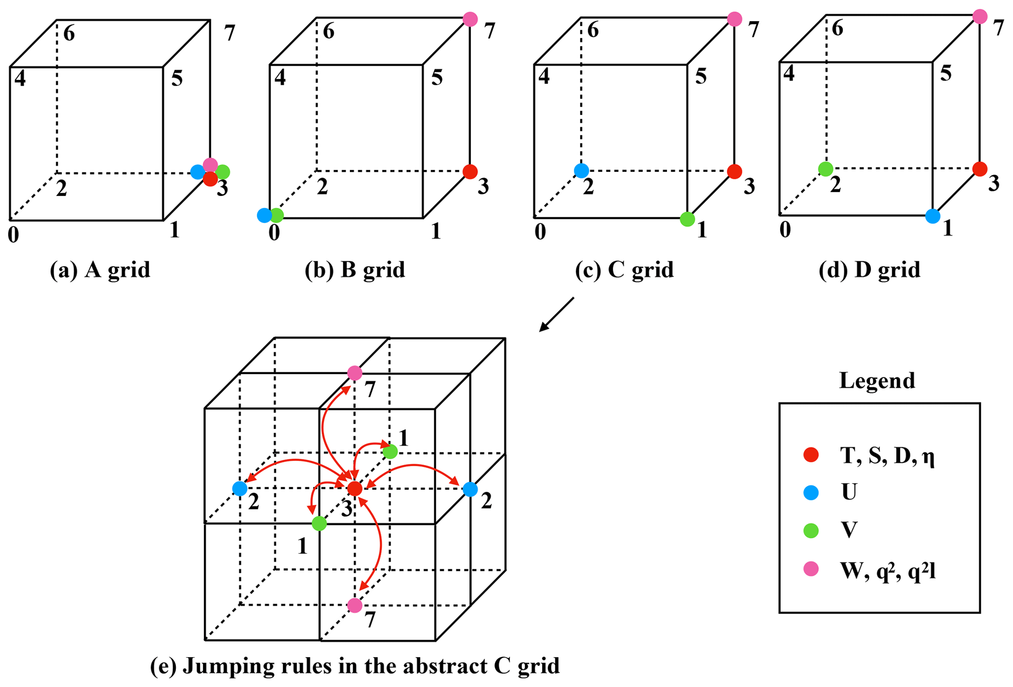
https://www.geosci-model-dev.net/12/4729/2019/gmd-12-4729-2019-f04

Figure 4The schematic diagram of the relative positions of the variables on the abstract staggered grid and the jumping procedures among the grid points.

Download

When we call the average and differential operators mentioned in Table 1, e.g., on the abstract Arakawa C grid, the position of Array D is point 3, and the average AXB operator acting on Array D will change the position from point 3 to point 1. Since Array U is also allocated at point 1, the operation AXB(D)⋅U is allowed. In addition, the subsequent differential operator on Array AXB(D)⋅U will change the position of Array DXF(AXB(D)⋅U) from point 1 to point 3.

The jumping rules of different operators are given in Table 2. Due to the design of the abstract staggered grids, the jumping rules for the Arakawa A, B, C, and D grids are fixed. A change in the position of an array is determined only by the direction of a certain operator acting on that array.

Table 2The jumping rules of an operator acting on an Array.

Download Print Version | Download XLSX

The grid type can be changed conveniently. For instance, if one would like to do so, only the following steps need to be taken. First the position information of each physical variable needs to be reset (shown in Fig. 4). Then the discrete form of each equation needs to be redesigned. We take the Eq. (1) switching from Arakawa C grid to Arakawa B grid as an example. The positions of the horizontal velocity Array U and Array V are changed to point 0; Array η and Array D stay the same. The discrete form is changed from Eq. (4) into Eq. (13), and the corresponding implementation by operators is changed from Eq. (6) into Eq. (14). By doing so, the transformation of grid types can be easily implemented.

\begin{matrix} (13) & \begin{aligned} \frac{η_{t + 1} (i, j) - η_{t - 1} (i, j)}{2 \cdot d t} \\ + \frac{1}{4 \cdot d x (i, j)^{*}} ((D (i + 1, j) + D (i, j)) \cdot (U (i + 1, j) \\ + U (i + 1, j + 1)) - (D (i, j) + D (i - 1, j)) \\ \cdot (U (i, j) + U (i, j + 1))) \\ + \frac{1}{4 \cdot d y (i, j)^{*}} ((D (i, j + 1) + D (i, j)) \\ \cdot (V (i, j + 1) + V (i + 1, j + 1)) \\ - (D (i, j) + D (i, j - 1)) \\ \cdot (V (i, j) + V (i + 1, j))) = 0, \end{aligned} \\ (14) & η_{t + 1} = η_{t - 1} - 2 \cdot d t \cdot (δ_{f}^{x} ({\overline{D}}_{b}^{x} \cdot {\overline{U}}_{f}^{y}) + δ_{f}^{y} ({\overline{D}}_{b}^{y} \cdot {\overline{V}}_{f}^{x})) . \end{matrix}

The position information and jumping rules are used to implicitly check whether the discrete form of an equation is correct. The grid increments are hidden by all the differential operators, thus it makes the code simple and clean. In addition, since the rules are suitable for multiple staggered Arakawa grids, the modelers can flexibly switch the ocean model between different Arakawa grids. Notably, the users of OpenArray should input the correct positions of each array in the initialization phase. The value of the position is an input parameter when declaring an Array. An error will be reported if an operation is performed between misplaced points.

Although most of the existing ocean models use finite difference or finite volume methods on structured or semi-structured meshes (e.g., Blumberg and Mellor, 1987; Shchepetkin and McWilliams, 2005), there are still some ocean models using unstructured meshes (e.g., Chen et al., 2003; Korn, 2017), and even the spectral element method (e.g., Levin et al., 2000). In our current work, we design the basic operators only for finite difference and finite volume methods with structured grids. More customized operators for the other numerical methods and meshes will be implemented in our future work.

3 Design of OpenArray

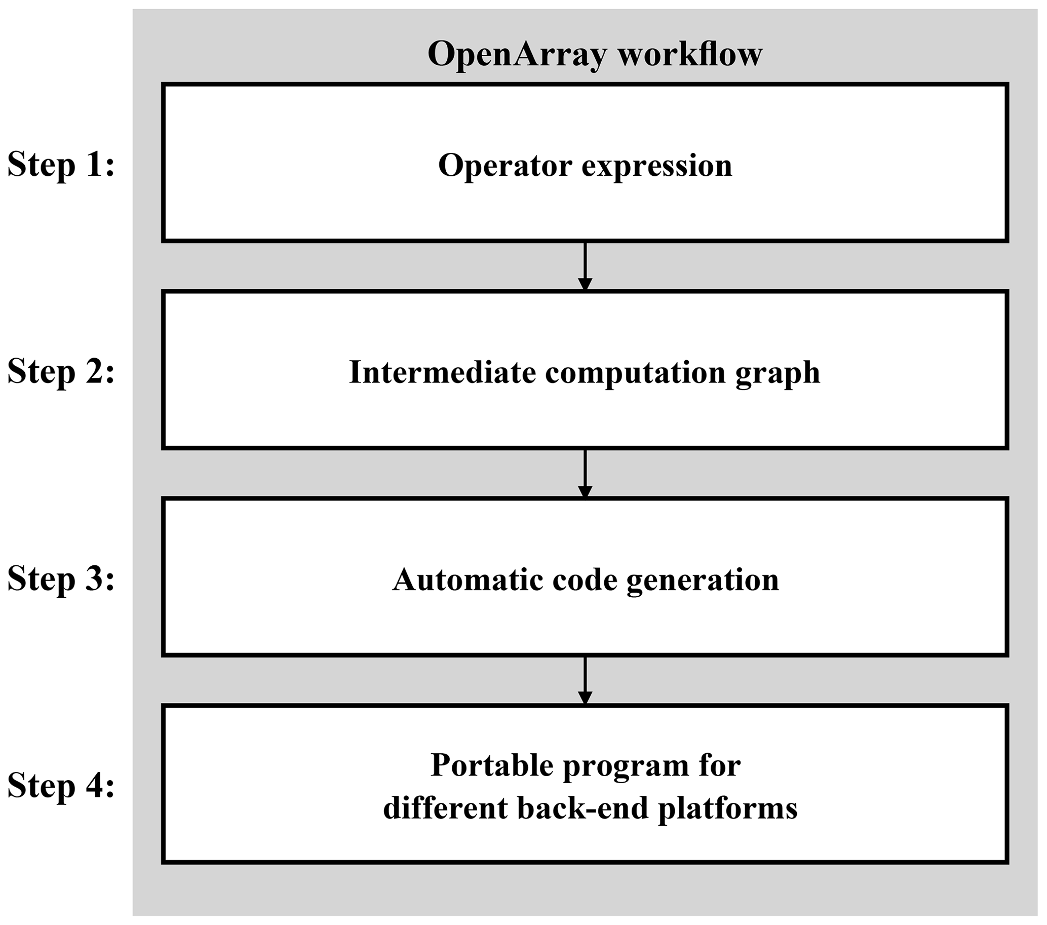
Through the above operator notations in Table 1, ocean modelers can quickly convert the discrete PDEs into the corresponding operator expression forms. The main purpose of OpenArray is to make complex parallel programming transparent to the modelers. As illustrated in Fig. 5, we use a computation graph as an intermediate representation, meaning that the operator expression forms written in Fortran will be translated into a computation graph with a particular data structure. In addition, OpenArray will use the intermediate computation graph to analyze the dependency of the distributed data and produce the underlying parallel code. Finally, we use stable and mature compilers, such as the GNU Compiler Collection (GCC), Intel compiler (ICC), and Sunway compiler (SWACC), to generate the executable programs according to different back-end platforms. These four steps and some related techniques are described in detail in this section.

https://www.geosci-model-dev.net/12/4729/2019/gmd-12-4729-2019-f05

Figure 5The workflow of OpenArray.

Download

3.1 Operator expression

Although the basic generalized operators listed in Table 1 are only suitable to execute 1st-order difference, other high-order difference or even more complicated operations can be combined by these basic operators. For example, a 2nd-order difference operation can be expressed as $δ_{f}^{x} (δ_{b}^{x} (var))$ . Supposing the grid distance is uniform, the corresponding discrete form is $[var (i + 1, j, k) + var (i - 1, j, k) - 2 \cdot var (i, j, k)] / d x^{2}$ . In addition, the central difference operation can be expressed as $(δ_{f}^{x} (var) + δ_{b}^{x} (var)) / 2$ since the corresponding discrete form is $[var (i + 1, j, k) - var (i - 1, j, k)] / 2 d x$ .

Using these operators to express the discrete PDE, the code and formula are very similar. We call this effect “the self-documenting code is the formula”. Figure 6 shows the one-to-one correspondence of each item in the code and the items in the sea surface elevation equation. The code is very easy to program and understand. Clearly, the basic operators and the combined operators greatly simplify the development and maintenance of ocean models. The complicated parallel and optimization techniques are hidden behind these operators. Modelers no longer need to care about details and can escape from the “parallelism swamp”, and can therefore concentrate on the scientific issues.

https://www.geosci-model-dev.net/12/4729/2019/gmd-12-4729-2019-f06

Figure 6The effect of “the self-documenting code is the formula” illustrated by the sea surface elevation equation.

Download

3.2 Intermediate computation graph

Considering the example mentioned in Fig. 6, if one needs to compute the term DXF(AXB(D)⋅u) with the traditional operator overloading method, one first computes AXB(D) and stores the result into a temporary array (named tmp1), and then executes (tmp1⋅u) and stores the result into a new array, tmp2. The last step is to compute DXF(tmp2) and store the result in a new array, tmp3. Numerous temporary arrays consume a considerable amount of memory, making the efficiency of operator overloading poor.

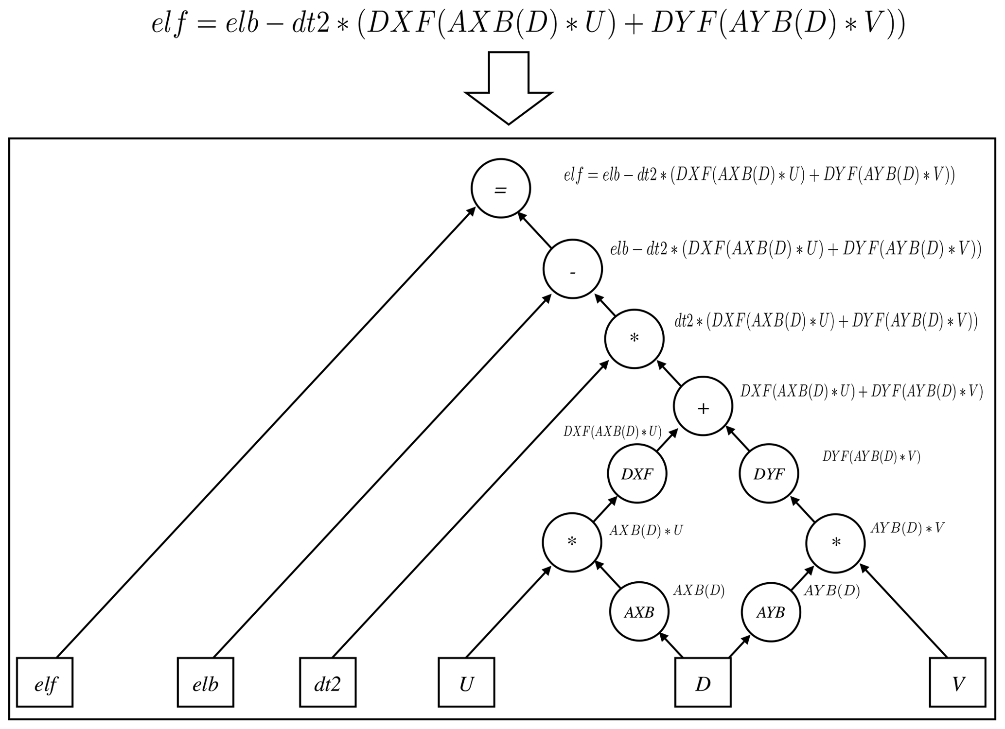
To solve this problem, we convert an operator expression form into a directed and acyclic graph, which consists of basic data and function nodes, to implement a so-called lazy expression evaluation (Bloss et al., 1988; Reynolds, 1999). Unlike the traditional operator overloading method, we overload all arithmetic functions to generate an intermediate computation graph rather than to obtain the result of each function. This method is widely used in deep-learning frameworks, e.g., TensorFlow (Abadi et al., 2016) and Theano (Bastien et al., 2012), to improve computing efficiency. Figure 7 shows the procedure of parsing the operator expression form of the sea level elevation equation into a computation graph. The input variables in the square boxes include the sea surface elevation (elb), the zonal velocity (u), the meridional velocity (v), and the depth (D). Variable dt2 is a constant equal to 2⋅dt. The final output is the sea surface elevation at the next time step (elf). The operators in the circles have been overloaded in OpenArray. In summary, all the operators provided by OpenArray are functions for the Array calculation, in which the “=” notation is the assignment function, the “–” notation is the subtraction function, the “*” notation is the multiplication function, the “+” notation is the addition function, DXF and DYF are the differential functions, and AXF and AYF are the average functions.

https://www.geosci-model-dev.net/12/4729/2019/gmd-12-4729-2019-f07

Figure 7Parsing the operator expression form into the computation graph.

Download

3.3 Code generation

Given a computation graph, we design a lightweight engine to generate the corresponding source code (Fig. 8). Each operator node in the computation graph is called a kernel. The sequence of all kernels in a graph is usually fused into a large kernel function. Therefore, the underlying engine schedules and executes the fused kernel once and obtains the final result directly without any auxiliary or temporary variables. Simultaneously, the scheduling overhead of the computation graph and the startup overhead of the basic kernels can be reduced.

https://www.geosci-model-dev.net/12/4729/2019/gmd-12-4729-2019-f08

Figure 8The schematic diagram of kernel fusion.

Download

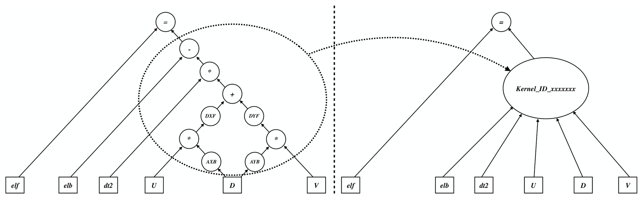
Most of the scientific computational applications are limited by the memory bandwidth and cannot fully exploit the computing power of a processor. Fortunately, kernel fusion is an effective optimization method to improve memory locality. When two kernels need to process some data, their fusion holds shared data in the memory. Prior to the kernel fusion, the computation graph is analyzed to find the operator nodes that can be fused, and the analysis results are stored in several subgraphs. Users can access any individual subgraph by assigning the subgraph to an intermediate variable for diagnostic purposes. After being given a series of subgraphs, the underlying engine dynamically generates the corresponding kernel function in C $+ +$ using just-in-time (JIT) compilation techniques (Suganuma and Yasue, 2005). The JIT compiler used in OpenArray can fuse numbers of operators into a large compiled kernel. The benefit of fusing operators is to alleviate memory bandwidth limitations and improve performance compared with executing operators one by one. In order to generate a kernel function based on a subgraph, we first add the function header and variable definitions according to the name and type in the Array structure. And then we add the loop head through the dimension information. Finally, we perform a depth-first walk on the expression tree to convert data, operators, and assignment nodes into a complete expression including load variables, arithmetic operation, and equal symbol with C $+ +$ language.

Notably, the time to compile a single kernel function is short but practical applications usually need to be run for thousands of time steps and the overhead of generating and compiling the kernel functions for the computation graph is extremely high. Therefore, we generate a fusion kernel function only once for each subgraph, and put it into a function pool. Later, when facing the same computation subgraph, we fetch the corresponding fusion kernel function directly from the pool.

Since the arrays in OpenArray are distributed among different processing units, and the operator needs to use the data in the neighboring points, to ensure the correctness it is necessary to check the data consistency before fusion. The use of different data-splitting methods for distributed arrays can greatly affect computing performance. The current data-splitting method in OpenArray is the widely used block-based strategy. Solving PDEs on structured grids often divides the simulated domain into blocks that are distributed to different processing units. However, the differential and average operators always require their neighboring points to perform array computations. Clearly, ocean modelers have to frequently call corresponding functions to carefully control the communication of the local boundary region.

Therefore, we implemented a general boundary management module to implicitly maintain and update the local boundary information so that the modelers no longer need to address the message communication. The boundary management module uses asynchronous communication to update and maintain the data of the boundary region, which is useful for simultaneous computing and communication. These procedures of asynchronous communication are implicitly invoked when calling the basic kernel or the fused kernel to ensure that the parallel details are completely transparent to the modelers. For the global boundary conditions of the limited physical domains, the values at the physical border are always set to zero within the operators and operator expressions. In realistic cases, the global boundary conditions are set by a series of functions (e.g., radiation, wall) provided by OpenArray.

3.4 Portable program for different back-end platforms

With the help of dynamic code generation and JIT compilation technology, OpenArray can be migrated to different back-end platforms. Several basic libraries, including Boost C $+ +$ libraries and Armadillo library, are required. The JIT compilation module is based on low-level virtual machine (LLVM), thus theoretically the module can only be ported to platforms supporting LLVM. If LLVM is not supported, as on the Sunway platform, one can generate the fusion kernels in advance by running the ocean model on an X86 platform. If the target platform uses CPUs with acceleration cards, such as GPU clusters, it is necessary to add control statements in the CPU code, including data transmission, calculation, synchronous, and asynchronous statements. In addition, the accelerating solution should involve the selection of the best parameters, e.g., “blockDim” and “gridDim” on GPU platforms. In short, the code generation module of OpenArray also needs to be refactored to be able to generate codes for different back-end platforms. The application based on OpenArray can then be migrated seamlessly to the target platform. Currently, we have designed the corresponding source code generation module for Intel CPU and Sunway processors in OpenArray.

According to the TOP500 list released in November 2018, the Sunway TaihuLight is ranked third in the world, with a LINPACK benchmark rating of 93 petaflops provided by Sunway many-core processors (or Sunway CPUs). As shown in Fig. 9, every Sunway CPU includes 260 processing elements (or cores) that are divided into four core groups. Each core group consists of 64 computing processing elements (CPEs) and a management processing element (MPE) (Qiao et al., 2017). CPEs handle large-scale computing tasks and the MPE is responsible for the task scheduling and communication. The relationship between MPE and CPE is like that between CPU and many-core accelerator, except that they are fused into a single Sunway processor sharing a unified memory space. To make the most of the computing resources of the Sunway TaihuLight, we generate kernel functions for the MPE, which is responsible for the thread control, and CPE, which performs the computations. The kernel functions are fully optimized with several code optimization techniques (Pugh, 1991) such as loop tiling, loop aligning, single-instruction multiple-date (SIMD) vectorization, and function inline. In addition, due to the high memory access latency of CPEs, we accelerate data access by providing instructions for direct memory access in the kernel to transfer data between the main memory and local memory (Fu et al., 2017).

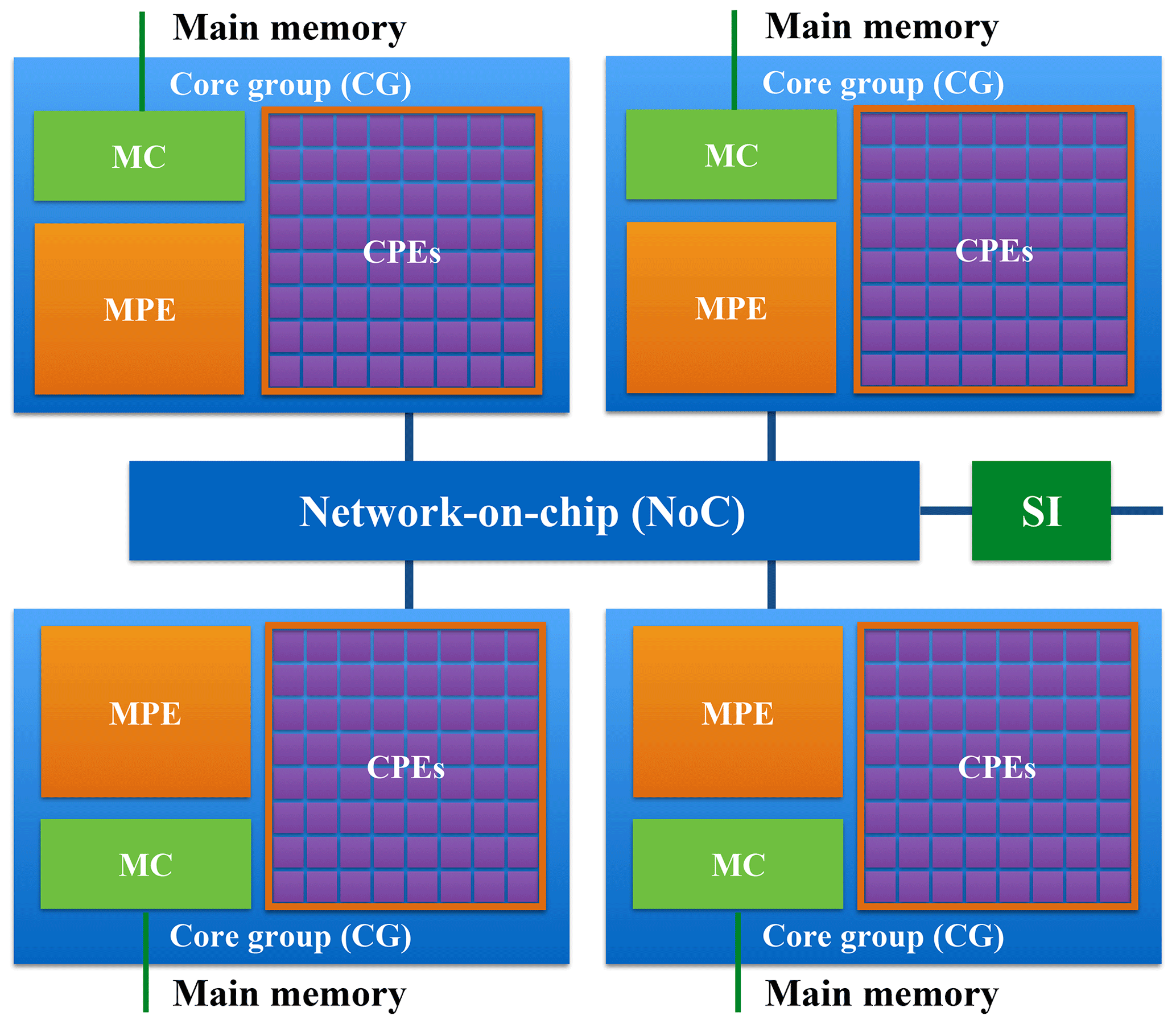
https://www.geosci-model-dev.net/12/4729/2019/gmd-12-4729-2019-f09

Figure 9The MPE–CPE hybrid architecture of the Sunway processor. Every Sunway processor includes 4 core groups (CGs) connected by the network-on-chip (NoC). Each CG consists of a management processing element (MPE), 64 computing processing elements (CPEs) and a memory controller (MC). The Sunway processor uses the system interface (SI) to connect with outside devices.

Download

4 Implementation of GOMO

In this section, we introduce how to implement a numerical ocean model using OpenArray. The most important step is to derive the primitive discrete governing equations in operator expression form, and then the following work is completed by OpenArray.

The fundamental equations of GOMO are derived from POM. GOMO features a bottom-following free-surface staggered Arakawa C grid. To effectively evolve the rapid surface fluctuations, GOMO uses the mode-splitting algorithm inherited from POM to address the fast-propagating surface gravity waves and slow-propagating internal waves in barotropic (external) and baroclinic (internal) modes, respectively. The details of the continuous governing equations, the corresponding operator expression form, and the descriptions of all the variables used in GOMO are listed in the appendices A–C, respectively.

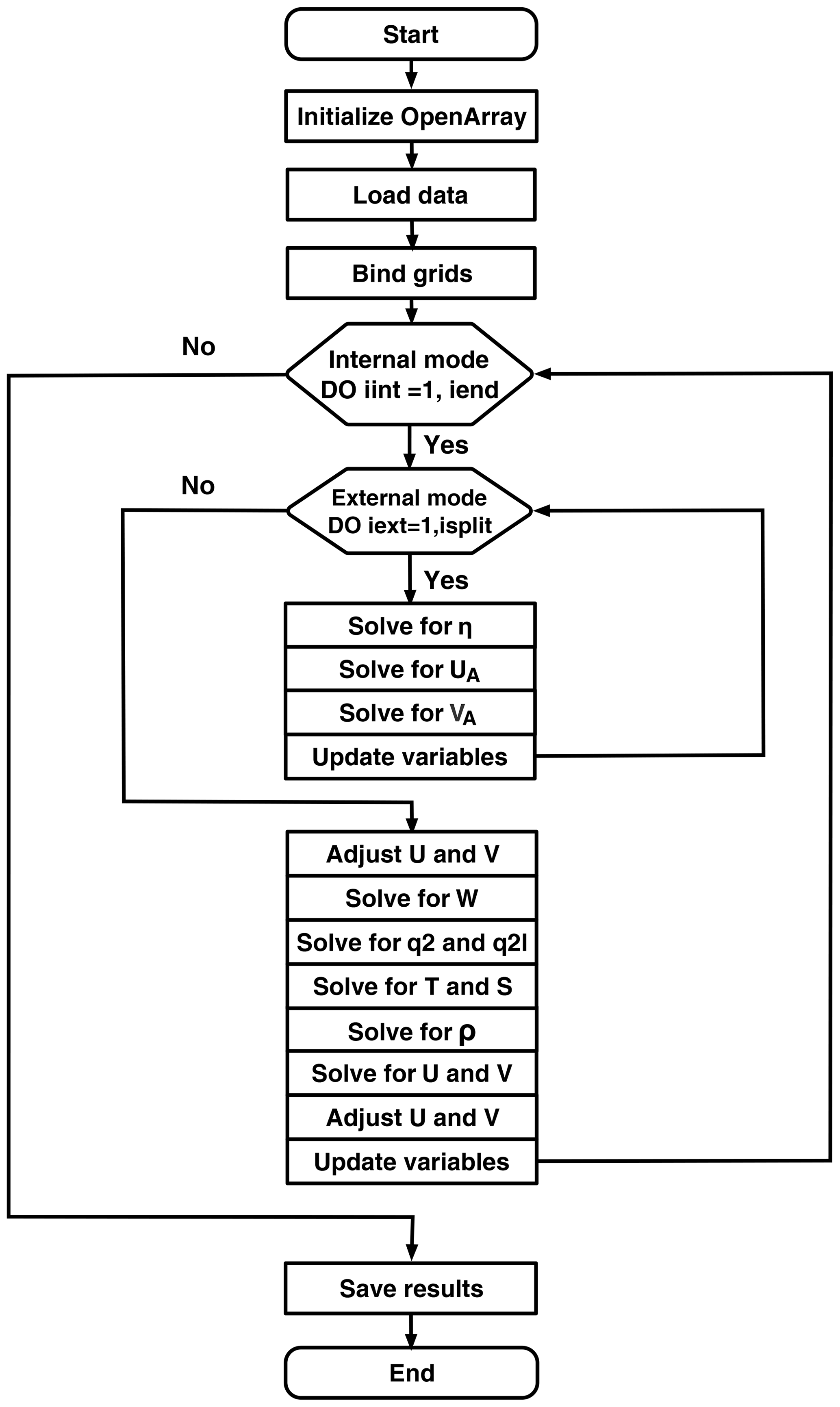
Figure 10 shows the basic flow diagram of GOMO. At the beginning, we initialize OpenArray to make all operators suitable for GOMO. After loading the initial values and the model parameters, the distance information is input into the differential operators through grid binding. In the external mode, the main consumption is computing the 2-D sea surface elevation η and column-averaged velocity (U_A, V_A). In the internal mode, 3-D array computations predominate in order to calculate baroclinic motions ( $U, V, W$ ), tracers ( $T, S, ρ$ ), and the turbulence closure scheme (q²,q²l) (Mellor and Yamada, 1982), where $U, V,$ and W are the velocity fields in the x, y, and σ directions and $T, S,$ and ρ are the potential temperature, the salinity, and the density, respectively. $q^{2} / 2,$ and q²l∕2 are the turbulence kinetic energy and production of turbulence kinetic energy with turbulence length scale, respectively.

https://www.geosci-model-dev.net/12/4729/2019/gmd-12-4729-2019-f10

Figure 10Flow diagram of GOMO.

Download

Table 3Comparing GOMO with several variations in the POM.

Download Print Version | Download XLSX

When the user dives into the GOMO code, the main time stepping loop in GOMO appears to run on a single processor. However, as described above, implicit parallelism is the most prominent feature of the program using OpenArray. The operators in OpenArray, not only the difference and average operators, but also the “+”, “–”, “*”, “/” and “=” operators in the Fortran code, are all overloaded for the special data structure “Array”. The seemingly serial Fortran code is implicitly converted to parallel C $+ +$ code by OpenArray, and the parallelization is hidden from the modelers.

Because the complicated parallel optimization and tuning processes are decoupled from the ocean modeling, we completely implemented GOMO based on OpenArray in only 4 weeks, whereas implementation may take several months or even longer when using the MPI or CUDA library.

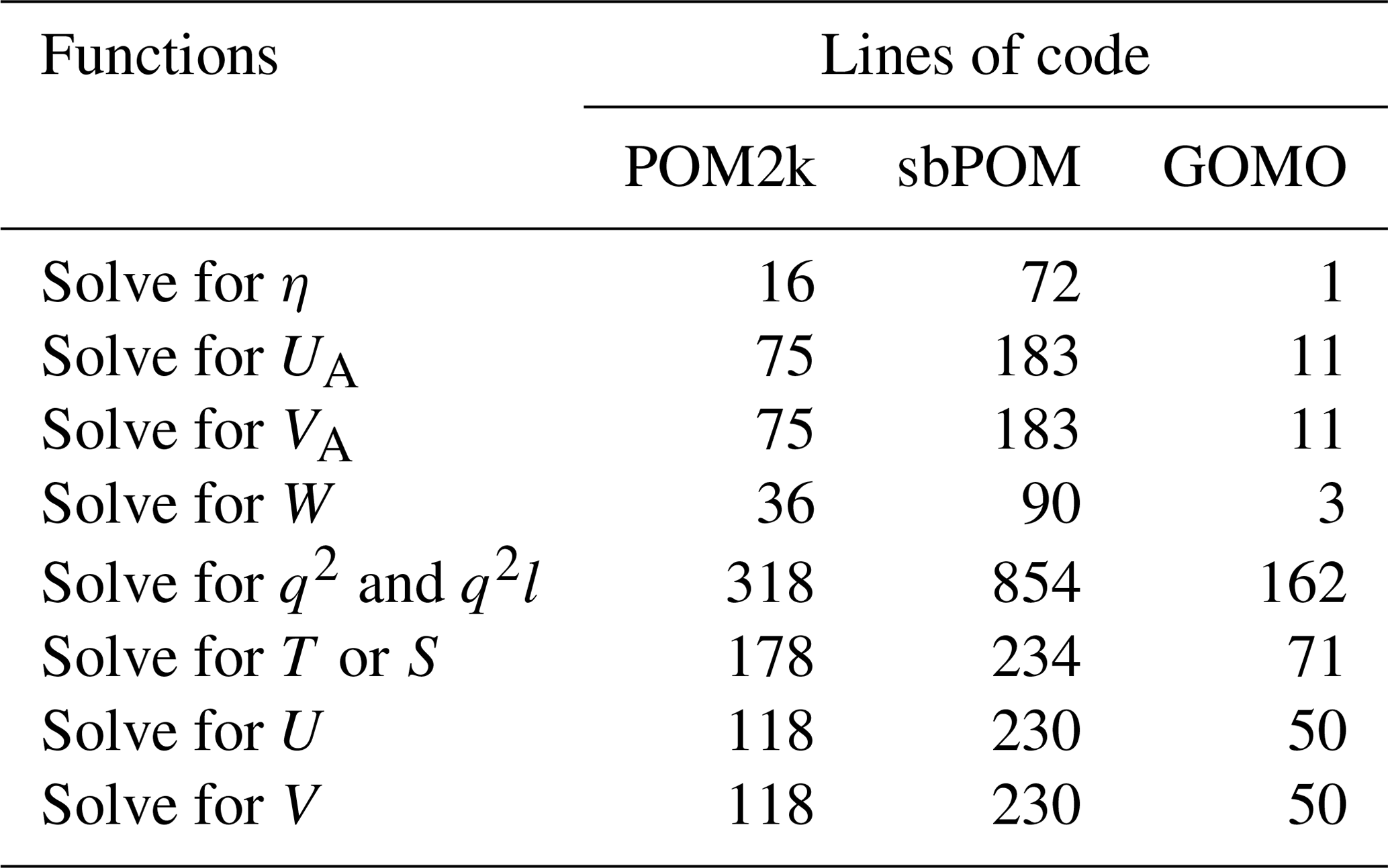
In comparison with the existing POM and its multiple variations, including (to name a few) Stony Brook Parallel Ocean Model (sbPOM), mpiPOM, and POMgpu, GOMO has less code but is more powerful in terms of compatibility. As shown in Table 3, the serial version of POM (POM2k) contains 3521 lines of code. Models sbPOM and mpiPOM are parallelized using MPI, while POMgpu is based on MPI and CUDA-C. The codes of sbPOM, mpiPOM, and POMgpu are extended to 4801, 9680, and 30 443 lines, respectively. In contrast, the code of GOMO is decreased to 1860 lines. Moreover, GOMO completes the same function as the other approaches while using the least amount of code (Table 4), since the complexity has been transferred to OpenArray, which includes about 11 800 lines of codes.

Table 4Comparison of the amount of code for different functions.

Download Print Version | Download XLSX

In addition, poor portability considerably restricts the use of advanced hardware in oceanography. With the advantages of OpenArray, GOMO is adaptable to different hardware architectures, such as the Sunway processor. The modelers do not need to modify any code when changing platforms, eliminating the heavy burden of transmitting code. As computing platforms become increasingly diverse and complex, GOMO becomes more powerful and attractive than the machine-dependent models.

5 Results

In this section, we first evaluate the basic performance of OpenArray using benchmark tests on a single CPU platform. After checking the correctness of GOMO through an ideal seamount test case, we use GOMO to further test the scalability and efficiency of OpenArray.

5.1 Benchmark testing

We choose two typical PDEs and their implementations from Rodinia v3.1, which is a benchmark suite for heterogeneous computing (Che et al., 2009), as the original version. For comparison, we re-implement these two PDEs using OpenArray. In addition, we added two other test cases. As shown in Table 5, the 2-D continuity equation is used to solve sea surface height, and its continuous form is shown in Eq. (1). The 2-D heat diffusion equation is a parabolic PDE that describes the distribution of heat over time in a given region. Hotspot is a thermal simulation used for estimating processor temperature on structured grids (Che et al., 2009; Huang et al., 2006). We tested one 2-D case (Hotspot2D) and one 3-D case (Hotspot3D) of this program. The average runtime for 100 iterations is taken as the performance metric. All tests are executed on a single workstation with an Intel Xeon E5-2650 CPU. The experimental results show that the performance of OpenArray versions is comparable to the original versions.

Table 5Four benchmark tests.

Download Print Version | Download XLSX

5.2 Validation tests of GOMO

The seamount problem proposed by Beckmann and Haidvogel is a widely used ideal test case for regional ocean models (Beckmann and Haidvogel, 1993). It is a stratified Taylor column problem which simulates the flow over an isolated seamount with a constant salinity and a reference vertical temperature stratification. An eastward horizontal current of 0.1 m s⁻¹ is added at model initialization. The southern and northern boundaries are closed. If the Rossby number is small, an obvious anticyclonic circulation is trapped by the mount in the deep water.

Using the seamount test case, we compare GOMO and sbPOM results. The configurations of both models are exactly the same. Figure 11 shows that GOMO and sbPOM both capture the anticyclonic circulation at 3500 m depth. The shaded plot shows the surface elevation, and the array plot shows the current at 3500 m. Panels 11a, b, and c show the results of GOMO, sbPOM, and the difference (GOMO-sbPOM), respectively. The differences in the surface elevation and deep currents between the two models are negligible (Fig. 11c).

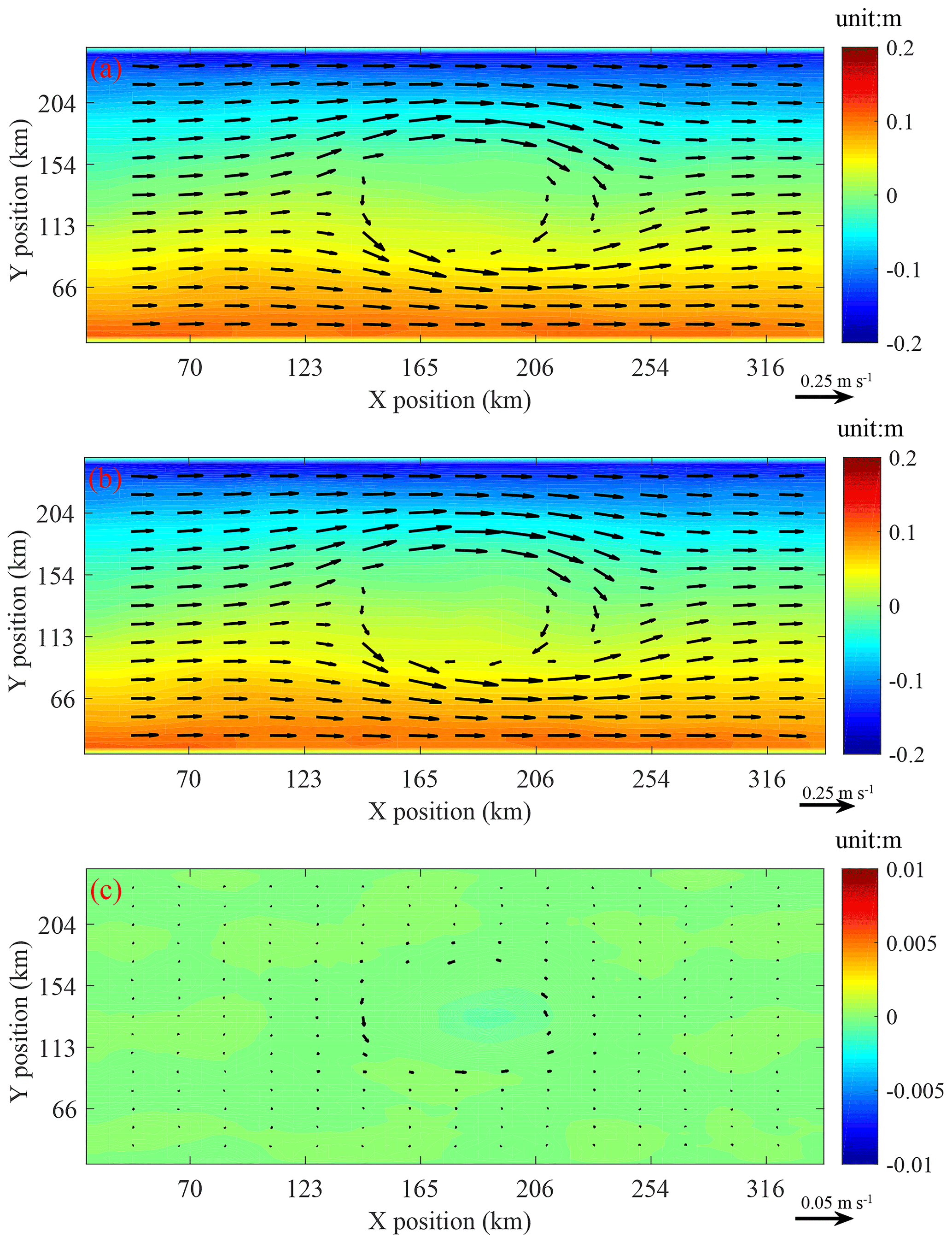
https://www.geosci-model-dev.net/12/4729/2019/gmd-12-4729-2019-f11

Figure 11Comparison of the surface elevation (shaded) and currents at 3500 m depth (vector) between GOMO and sbPOM on the 4th model day. (a) GOMO, (b) sbPOM, and (c) GOMO-sbPOM.

Download

5.3 The weak and strong scalability of GOMO

The seamount test case is used to compare the performance of sbPOM and GOMO in a parallel environment. We use the X86 cluster at the National Supercomputing Center in Wuxi, China, which provides 5000 Intel Xeon E5-2650 v2 CPUs for our account at most. Figure 12a shows the result of a strong scaling evaluation, in which the model size is fixed at $2048 \times 2048 \times 50$ . The dashed line indicates the ideal speedup. For the largest parallelism with 4096 processes, GOMO and sbPOM achieve 91 % and 92 % parallel efficiency, respectively. Figure 12b shows the weak scalability of sbPOM and GOMO. In the weak scaling test, the model size for each process is fixed at $128 \times 128 \times 50$ , and the number of processes is gradually increased from 16 to 4096. Taking the performance of 16 processes as a baseline, we determine that the parallel efficiencies of GOMO and sbPOM using 4096 processes are 99.0 % and 99.2 %, respectively.

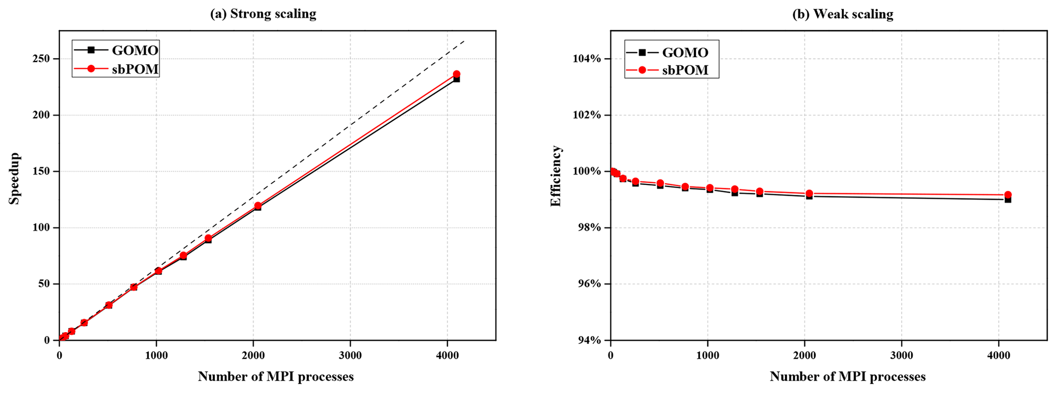
https://www.geosci-model-dev.net/12/4729/2019/gmd-12-4729-2019-f12

Figure 12Performance comparison between sbPOM and GOMO on the X86 cluster. Panels (a) shows the strong scaling result; vertical axis denotes the speedup relative to 16 processes in a single node. Panel (b) shows the weak scaling result.

Download

5.4 Testing on the Sunway platform

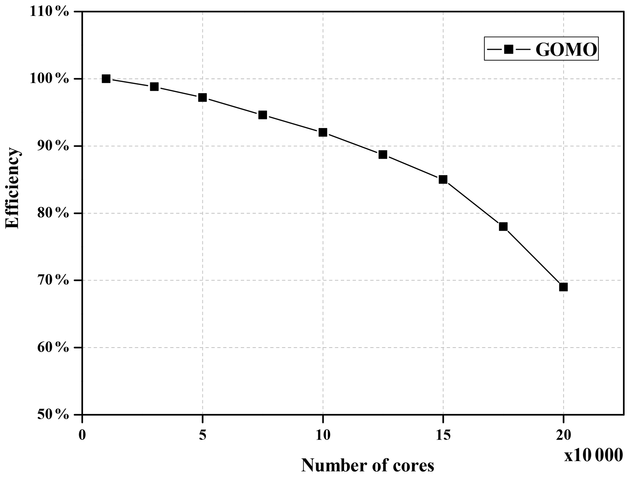
We also test the scalability of GOMO on the Sunway platform. Supposing that the baseline is the runtime of GOMO at 10 000 Sunway cores with a grid size of $4096 \times 4096 \times 50$ , the parallel efficiency of GOMO can still reach 85 % at 150 000 cores, as shown in Fig. 13. However, we notice that the scalability declines sharply when the number of cores exceeds 150 000. There are two reasons leading to this decline. First, the block size assigned to each core decreases as the number of cores increases, causing more communication during boundary region updating. Second, some processes cannot be accelerated even though more computing resources are available; for example, the time spent on creating the computation graph, generating the fusion kernels, and compiling the JIT cannot be reduced. Even though the fusion-kernel codes are generated and compiled only once at the beginning of a job, it consumes about 2 min. In a sense, OpenArray performs better when processing large-scale data, and GOMO is more suitable for high-resolution scenarios. In the future, we will further optimize the communication and graph-creating modules to improve the efficiency for large-scale cores.

https://www.geosci-model-dev.net/12/4729/2019/gmd-12-4729-2019-f13

Figure 13Parallel efficiency of GOMO on the Sunway platform.

Download

6 Discussion

As we mentioned in Sect. 1, the advantages of OpenArray are its ease of use, high efficiency, and portability. Using OpenArray, modelers without any parallel computing skill or experience can write simple operator expressions in Fortran to implement complex ocean models. The ocean models can be run on any CPU or Sunway platforms which have deployed the OpenArray library. We call this effect “write once, run everywhere”. Other similar libraries (e.g., ATMOL, ICON DSL, STELLA, and COARRAY) require users to manually control the boundary communication and task scheduling to some extent. In contrast, OpenArray implements completely implicit parallelism with user-friendly interfaces and programming languages.

However, there are still several problems to be solved in the development of OpenArray. The first issue is computational efficiency. Once a variable is in one of the processor registers or in the highest speed cache, it should be used as much as possible before being replaced. In fact, we should never move variables more than once each time step. The memory consumption brought by overloading techniques is usually high due to the unnecessary variable moving and unavoidable cache missing. The current efficiency and scalability of GOMO are close to sbPOM since we have adopted a series of optimization methods, such as memory pool, graph computing, JIT compilation, and vectorization, to alleviate the requirement of memory bandwidth. However, we have to admit that we cannot fully solve the memory bandwidth limit problem at present. We think that time skewing is a cache-oblivious algorithm for stencil computations (Frigo and Strumpen, 2005) since it can exploit temporal locality optimally throughout the entire memory hierarchy. In addition, the polyhedral model may be another potential approach, which uses an abstract mathematical representation based on integer polyhedral to analyze and optimize the memory access pattern of a program.

The second issue is that the current OpenArray version cannot support customized operators. When modelers try out another higher-order advection or any other numerical scheme, the 12 basic operators provided by OpenArray are not abundant. We considered using a template mechanism to support the customized operators. The rules of operations are defined in a template file, where the calculation form of each customized operator is described by a regular expression. If users want to add a customized operator, they only need to append a regular expression into the template file.

OpenArray and GOMO will continue to be developed, and the following three key improvements are planned for the following years.

First, we are developing the GPU version of OpenArray. During the development, the principle is to keep hot data in GPU memory or directly swapping between GPUs and avoid returning data to the main CPU memory. NVLink provides high bandwidth and outstanding scalability for GPU-to-CPU or GPU-to-GPU communication and addresses the interconnect issue for multi-GPU and multi-GPU/CPU systems.

Second, the data input/output is becoming a bottleneck of earth system models as the resolution increases rapidly. At present we encapsulate the PnetCDF library to provide simple I/O interfaces, such as load operation and store operation. A climate fast input/output (CFIO) library (Huang et al., 2014) will be implemented into OpenArray in the next few years. The performance of CFIO is approximately 220 % faster than PnetCDF because of the overlapping of I/O and computing. CFIO will be merged into the future version of OpenArray and the performance is expected to be further improved.

Finally, as for most of the ocean models, GOMO also faces the load imbalance issue. We are adding the more effective load balance schemes, including space-filling curve (Dennis, 2007) and curvilinear orthogonal grids, into OpenArray in order to reduce the computational cost on land points.

OpenArray is a product of the collaboration between oceanographers and computer scientists. It plays an important role in simplify the porting work on the Sunway TaihuLight supercomputer. We believe that OpenArray and GOMO will continue to be maintained and upgraded. We aim to promote it to the model community as a development tool for future numerical models.

7 Conclusions

In this paper, we design a simple computing library (OpenArray) to decouple ocean modeling and parallel computing. OpenArray provides 12 basic operators that are abstracted from PDEs and extended to ocean model governing equations. These operators feature user-friendly interfaces and an implicit parallelization ability. Furthermore, some state-of-the-art optimization mechanisms, including computation graphing, kernel fusion, dynamic source code generation, and JIT compiling, are applied to boost the performance. The experimental results prove that the performance of a program using OpenArray is comparable to that of well-designed programs using Fortran. Based on OpenArray, we implement a numerical ocean model (GOMO) with high productivity, enhanced readability, and excellent scalable performance. Moreover, GOMO shows high scalability on both CPU systems and the Sunway platform. Although more realistic tests are needed, OpenArray may signal the beginning of a new frontier in future ocean modeling through ingesting basic operators and cutting-edge computing techniques.

Code availability

The source codes of OpenArray v1.0 are available at https://github.com/hxmhuang/OpenArray (Huang et al., 2019a), and the user manual of OpenArray can be accessed at https://github.com/hxmhuang/OpenArray/tree/master/doc (Huang et al., 2019b). GOMO is available at https://github.com/hxmhuang/GOMO (Huang et al., 2019c).

Appendix A: Continuous governing equations

The equations governing the baroclinic (internal) mode in GOMO are the 3-dimensional hydrostatic primitive equations.

\begin{matrix} (A1) & \frac{\partial η}{\partial t} + \frac{\partial U D}{\partial x} + \frac{\partial V D}{\partial y} + \frac{\partial W}{\partial σ} = 0, \\ (A2) & \begin{aligned} \frac{\partial U D}{\partial t} + \frac{\partial U^{2} D}{\partial x} + \frac{\partial U V D}{\partial y} + \frac{\partial U W}{\partial σ} \\ - f V D + g D \frac{\partial η}{\partial x} = \frac{\partial}{\partial σ} (\frac{K_{M}}{D} \frac{\partial U}{\partial σ}) \\ + \frac{g D^{2}}{ρ_{0}} \frac{\partial}{\partial x} \int_{σ}^{0} ρ d σ^{'} - \frac{g D}{ρ_{0}} \frac{\partial D}{\partial x} \int_{σ}^{0} σ^{'} \frac{\partial ρ}{\partial σ^{'}} d σ^{'} + F_{u}, \end{aligned} \\ (A3) & \begin{aligned} \frac{\partial V D}{\partial t} + \frac{\partial U V D}{\partial x} + \frac{\partial V^{2} D}{\partial y} + \frac{\partial V W}{\partial σ} + f U D \\ + g D \frac{\partial η}{\partial y} = \frac{\partial}{\partial σ} (\frac{K_{M}}{D} \frac{\partial V}{\partial σ}) + \frac{g D^{2}}{ρ_{0}} \frac{\partial}{\partial y} \int_{σ}^{0} ρ d σ^{'} \\ - \frac{g D}{ρ_{0}} \frac{\partial D}{\partial y} \int_{σ}^{0} σ^{'} \frac{\partial ρ}{\partial σ^{'}} d σ^{'} + F_{v}, \end{aligned} \\ (A4) & \begin{aligned} \frac{\partial T D}{\partial t} + \frac{\partial T U D}{\partial x} + \frac{\partial T V D}{\partial y} + \frac{\partial T W}{\partial σ} = \frac{\partial}{\partial σ} (K_{H} \frac{\partial T}{\partial σ}) \\ + F_{T} + \frac{\partial R}{\partial σ}, \end{aligned} \\ (A5) & \begin{aligned} \frac{\partial S D}{\partial t} + \frac{\partial S U D}{\partial x} + \frac{\partial S V D}{\partial y} + \frac{\partial S W}{\partial σ} = \\ \frac{\partial}{\partial σ} (K_{H} \frac{\partial S}{\partial σ}) + F_{S}, \end{aligned} \\ (A6) & ρ = ρ (T S p), \\ (A7) & \begin{aligned} \frac{\partial q^{2} D}{\partial t} + \frac{\partial U q^{2} D}{\partial x} + \frac{\partial V q^{2} D}{\partial y} + \frac{\partial W q^{2}}{\partial σ} = \\ \frac{\partial}{\partial σ} (\frac{K_{q}}{D} \frac{\partial q^{2}}{\partial σ}) + \frac{2 K_{M}}{D} [{(\frac{\partial U}{\partial σ})}^{2} + {(\frac{\partial V}{\partial σ})}^{2}] \\ + \frac{2 g}{ρ_{0}} K_{H} \frac{\partial ρ}{\partial σ} - \frac{2 D q^{3}}{B_{1} l} + F_{q^{2}}, \end{aligned} \end{matrix}

\begin{matrix} (A9) & \begin{aligned} \frac{\partial q^{2} l D}{\partial t} + \frac{\partial U q^{2} l D}{\partial x} + \frac{\partial V q^{2} l D}{\partial y} + \frac{\partial W q^{2} l}{\partial σ} = \\ \frac{\partial}{\partial σ} (\frac{K_{q}}{D} \frac{\partial q^{2} l}{\partial σ}) + E_{1} l \{\frac{K_{M}}{D} [{(\frac{\partial U}{\partial σ})}^{2} + {(\frac{\partial V}{\partial σ})}^{2}] \\ + \frac{g E_{3}}{ρ_{0}} K_{H} \frac{\partial ρ}{\partial σ}\} \tilde{W} - \frac{D q^{3}}{B_{1}} + F_{q^{2} l}, \end{aligned} \end{matrix}

where F_u, F_v, $F_{q^{2}}$ , and $F_{q^{2} l}$ are horizontal kinematic viscosity terms of u, v, q², and q²l, respectively. F_T and F_S are horizontal diffusion terms of T and S, respectively. $\tilde{W}$ is the wall proximity function.

\begin{matrix} (A10) & F_{u} = \frac{\partial}{\partial x} (2 A_{M} D \frac{\partial U}{\partial x}) + \frac{\partial}{\partial y} [A_{M} D (\frac{\partial U}{\partial y} + \frac{\partial V}{\partial x})], \\ (A11) & F_{v} = \frac{\partial}{\partial y} (2 A_{M} D \frac{\partial V}{\partial y}) + \frac{\partial}{\partial x} [A_{M} D (\frac{\partial U}{\partial y} + \frac{\partial V}{\partial x})], \\ (A12) & F_{T} = \frac{\partial}{\partial x} (A_{H} H \frac{\partial T}{\partial x}) + \frac{\partial}{\partial y} (A_{H} H \frac{\partial T}{\partial y}), \\ (A13) & F_{S} = \frac{\partial}{\partial x} (A_{H} H \frac{\partial S}{\partial x}) + \frac{\partial}{\partial y} (A_{H} H \frac{\partial S}{\partial y}), \\ (A14) & F_{q^{2}} = \frac{\partial}{\partial x} (A_{M} H \frac{\partial q^{2}}{\partial x}) + \frac{\partial}{\partial y} (A_{M} H \frac{\partial q^{2}}{\partial y}), \\ (A15) & F_{q^{2} l} = \frac{\partial}{\partial x} (A_{M} H \frac{\partial q^{2} l}{\partial x}) + \frac{\partial}{\partial y} (A_{M} H \frac{\partial q^{2} l}{\partial y}), \\ (A16) & \tilde{W} = 1 + \frac{E_{2} l}{κ} (\frac{1}{η - z} + \frac{1}{H - z}) . \end{matrix}

The equations governing the barotropic (external) mode in GOMO are obtained by vertically integrating the baroclinic equations.

\begin{matrix} (A17) & \frac{\partial η}{\partial t} + \frac{\partial U_{A} D}{\partial x} + \frac{\partial V_{A} D}{\partial y} = 0, \\ (A18) & \begin{aligned} \frac{\partial U_{A} D}{\partial t} + \frac{\partial (U_{A})^{2} D}{\partial x} + \frac{\partial U_{A} V_{A} D}{\partial y} - f V_{A} D \\ + g D \frac{\partial η}{\partial x} = {\tilde{F}}_{u_{a}} - w u (0) + w u (- 1) \\ - \frac{g D}{ρ_{0}} \int_{- 1}^{0} \int_{σ}^{0} [D \frac{\partial ρ}{\partial x} - \frac{\partial D}{\partial x} σ^{'} \frac{\partial ρ}{\partial σ}] d σ^{'} d σ + G_{u_{a}}, \end{aligned} \\ (A19) & \begin{aligned} \frac{\partial V_{A} D}{\partial t} + \frac{\partial U_{A} V_{A} D}{\partial y} + \frac{\partial (V_{A})^{2} D}{\partial y} + f U_{A} D \\ + g D \frac{\partial η}{\partial y} = {\tilde{F}}_{v_{a}} - w v (0) + w v (- 1) \\ - \frac{g D}{ρ_{0}} \int_{- 1}^{0} \int_{σ}^{0} [D \frac{\partial ρ}{\partial y} - \frac{\partial D}{\partial y} σ^{'} \frac{\partial ρ}{\partial σ}] d σ^{'} d σ + G_{v_{a}}, \end{aligned} \end{matrix}

where ${\tilde{F}}_{u_{a}}$ and ${\tilde{F}}_{v_{a}}$ are the horizontal kinematic viscosity terms of U_A and V_A, respectively. $G_{u_{a}}$ and $G_{v_{a}}$ are the dispersion terms of U_A and V_A, respectively. The subscript “A” denotes vertical integration.

\begin{matrix} (A20) & \begin{aligned} {\tilde{F}}_{u_{a}} = \frac{\partial}{\partial x} [2 H (A A_{M}) \frac{\partial U_{A}}{\partial x}] \\ + \frac{\partial}{\partial y} [H (A A_{M}) (\frac{\partial U_{A}}{\partial y} + \frac{\partial V_{A}}{\partial x})], \end{aligned} \\ (A21) & \begin{aligned} {\tilde{F}}_{v_{a}} = \frac{\partial}{\partial y} [2 H (A A_{M}) \frac{\partial V_{A}}{\partial y}] \\ + \frac{\partial}{\partial x} [H (A A_{M}) (\frac{\partial U_{A}}{\partial y} + \frac{\partial V_{A}}{\partial x})], \end{aligned} \\ (A22) & \begin{aligned} G_{u_{a}} = \frac{\partial^{2} (U_{A})^{2} D}{\partial x^{2}} + \frac{\partial^{2} U_{A} V_{A} D}{\partial x \partial y} - {\tilde{F}}_{u_{a}} \\ - \frac{\partial^{2} (U^{2})_{A} D}{\partial x^{2}} - \frac{\partial^{2} (U V)_{A} D}{\partial y^{2}} + (F_{u})_{A}, \end{aligned} \\ (A23) & \begin{aligned} G_{v_{a}} = \frac{\partial^{2} U_{A} V_{A} D}{\partial x \partial y} + \frac{\partial^{2} (V_{A})^{2} D}{\partial y^{2}} - {\tilde{F}}_{v_{a}} \\ - \frac{\partial^{2} (U V)_{A} D}{\partial x^{2}} - \frac{\partial^{2} (V^{2})_{A} D}{\partial y^{2}} + (F_{v})_{A}, \end{aligned} \\ (A24) & U_{A} = \int_{- 1}^{0} U d σ, \\ (A25) & V_{A} = \int_{- 1}^{0} V d σ, \\ (A26) & (U^{2})_{A} = \int_{- 1}^{0} U^{2} d σ, \\ (A27) & (U V)_{A} = \int_{- 1}^{0} U V d σ, \\ (A28) & (V^{2})_{A} = \int_{- 1}^{0} V^{2} d σ, \\ (A29) & (F_{u})_{A} = \int_{- 1}^{0} F_{u} d σ, \\ (A30) & (F_{v})_{A} = \int_{- 1}^{0} F_{v} d σ, \\ (A31) & A A_{M} = \int_{- 1}^{0} (A_{M}) d σ . \end{matrix}

Appendix B: Discrete governing equations

The discrete governing equations of baroclinic (internal) mode expressed by operators are shown as below:

\begin{matrix} (B1) & \frac{η^{t + 1} - η^{t - 1}}{2 d t i} + δ_{f}^{x} ({\overline{D}}_{b}^{x} U) + δ_{f}^{y} ({\overline{D}}_{b}^{y} V) + δ_{f}^{z} (W) = 0, \\ (B2) & \begin{aligned} \frac{({\overline{D}}_{b}^{x} U)^{t + 1} - ({\overline{D}}_{b}^{x} U)^{t - 1}}{2 d t i} + δ_{b}^{x} [({\overline{{\overline{D}}_{b}^{x} U)}}_{f}^{x} {\overline{U}}_{f}^{x}] \\ + δ_{f}^{y} [{\overline{({\overline{D}}_{b}^{y} V)}}_{b}^{x} {\overline{U}}_{b}^{y}] + δ_{f}^{z} ({\overline{W}}_{b}^{x} {\overline{U}}_{b}^{z}) - {\overline{(\tilde{f} {\overline{V}}_{f}^{y} D)}}_{b}^{x} \\ - {\overline{(f {\overline{V}}_{f}^{y} D)}}_{b}^{x} + g {\overline{D}}_{b}^{x} δ_{b}^{x} (η) = δ_{b}^{z} [\frac{{\overline{K}}_{M_{b}}^{x}}{({\overline{D}}_{b}^{x})^{t + 1}} δ_{f}^{z} (U^{t + 1})] \\ + \frac{g ({\overline{D}}_{b}^{x})^{2}}{ρ_{0}} \int_{σ}^{0} [δ_{b}^{x} ({\overline{ρ}}_{b}^{z}) - \frac{σ δ_{b}^{x} (D)}{{\overline{D}}_{b}^{x}} δ_{b}^{z} ({\overline{ρ}}_{b}^{x})] d σ^{'} + F_{u}, \end{aligned} \\ (B3) & \begin{aligned} \frac{({\overline{D}}_{b}^{y} V)^{t + 1} - ({\overline{D}}_{b}^{y} V)^{t - 1}}{2 d t i} + δ_{f}^{x} [({\overline{{\overline{D}}_{b}^{x} U)}}_{b}^{y} {\overline{V}}_{b}^{x}] \\ + δ_{b}^{y} [{\overline{({\overline{D}}_{b}^{y} V)}}_{f}^{y} {\overline{V}}_{f}^{y}] + δ_{f}^{z} ({\overline{W}}_{b}^{y} {\overline{V}}_{b}^{z}) + {\overline{(\tilde{f} {\overline{U}}_{f}^{x} D)}}_{b}^{y} \\ + {\overline{(f {\overline{U}}_{f}^{x} D)}}_{b}^{y} + g {\overline{D}}_{b}^{y} δ_{b}^{y} (η) = δ_{b}^{z} [\frac{{\overline{K}}_{M_{b}}^{y}}{({\overline{D}}_{b}^{y})^{t + 1}} δ_{f}^{z} (V^{t + 1})] \\ + \frac{g ({\overline{D}}_{b}^{y})^{2}}{ρ_{0}} \int_{σ}^{0} [δ_{b}^{y} ({\overline{ρ}}_{b}^{z}) - \frac{σ δ_{b}^{y} (D)}{{\overline{D}}_{b}^{y}} δ_{b}^{z} ({\overline{ρ}}_{b}^{y})] d σ^{'} + F_{v}, \end{aligned} \\ (B4) & \begin{aligned} \frac{(T D)^{t + 1} - (T D)^{t - 1}}{2 d t i} + δ_{f}^{x} ({\overline{T}}_{b}^{x} U {\overline{D}}_{b}^{x}) + δ_{f}^{y} ({\overline{T}}_{b}^{y} V {\overline{D}}_{b}^{y}) \\ + δ_{f}^{z} ({\overline{T}}_{b}^{z} W) = δ_{b}^{z} [\frac{K_{H}}{D^{t + 1}} δ_{f}^{z} (T^{t + 1})] + F_{T} + δ_{f}^{z} R, \end{aligned} \\ (B5) & \begin{aligned} \frac{(S D)^{t + 1} - (S D)^{t - 1}}{2 d t i} + δ_{f}^{x} ({\overline{S}}_{b}^{x} U {\overline{D}}_{b}^{x}) \\ + δ_{f}^{y} ({\overline{S}}_{b}^{y} V {\overline{D}}_{b}^{y}) + δ_{f}^{z} ({\overline{S}}_{b}^{z} W) = \\ δ_{b}^{z} [\frac{K_{H}}{D^{t + 1}} δ_{f}^{z} (S^{t + 1})] + F_{S}, \end{aligned} \\ (B6) & ρ = ρ (T S p), \\ (B7) & \begin{aligned} \frac{(q^{2} D)^{t + 1} - (q^{2} D)^{t - 1}}{2 d t i} + δ_{f}^{x} ({\overline{U}}_{b}^{z} {\overline{(q^{2})_{b}}}^{x} {\overline{D_{b}}}^{x}) \\ + δ_{f}^{y} ({\overline{V_{b}}}^{z} {\overline{(q^{2})_{b}}}^{y} {\overline{D_{b}}}^{y}) + δ_{f}^{z} {\overline{(W q^{2})}}_{b}^{z} = \\ δ_{b}^{z} [\frac{{\overline{(K_{q})_{f}}}^{z}}{D^{t + 1}} δ_{f}^{z} (q^{2})^{t + 1}] + \frac{2 K_{M}}{D} \{{[δ_{b}^{z} ({\overline{U}}_{f}^{x})]}^{2} \\ + {[δ_{b}^{z} ({\overline{V}}_{f}^{y})]}^{2}\} + \frac{2 g}{ρ_{0}} K_{H} δ_{b}^{z} (ρ) - \frac{2 D q^{3}}{B_{1} l} + F_{q^{2}}, \end{aligned} \end{matrix}

\begin{matrix} (B8) & \begin{aligned} \frac{(q^{2} l D)^{t + 1} - (q^{2} l D)^{t - 1}}{2 d t i} + δ_{f}^{x} ({\overline{U}}_{b}^{z} {\overline{(q^{2} l)}}_{b}^{x} {\overline{D}}_{b}^{x}) \\ + δ_{f}^{y} ({\overline{V}}_{b}^{z} {\overline{q^{2} l}}_{b}^{y} {\overline{D}}_{b}^{y}) + δ_{f}^{z} {\overline{(W q^{2} l)}}_{b}^{z} = \\ δ_{b}^{z} [\frac{{\overline{(K_{q})_{f}}}^{z}}{D^{t + 1}} δ_{f}^{z} (q^{2} l)^{t + 1}] + l E_{1} \frac{K_{M}}{D} \{{[δ_{b}^{z} ({\overline{U}}_{f}^{x})]}^{2} \\ + {[δ_{b}^{z} ({\overline{V}}_{f}^{y})]}^{2}\} \tilde{W} + \frac{l E_{1} E_{3} g}{ρ_{0}} K_{H} δ_{b}^{z} (ρ) \tilde{W} - \frac{D q^{3}}{B_{1}} \\ + F_{q^{2} l}, \end{aligned} \end{matrix}

where F_u, F_v, $F_{q^{2}}$ , and $F_{q^{2} l}$ are horizontal kinematic viscosity terms of u, v, q², and q²l, respectively. F_T and F_S are horizontal diffusion terms of T and S, respectively.

\begin{matrix} (B9) & \begin{aligned} F_{u} = δ_{b}^{x} [2 A_{M} D δ_{f}^{x} (U^{t - 1})] \\ + δ_{f}^{y} \{{\overline{({\overline{(A_{M})}}_{b}^{x})}}_{b}^{y} {\overline{({\overline{D}}_{b}^{x})}}_{b}^{y} [δ_{b}^{x} (V^{t - 1}) + δ_{b}^{y} (U^{t - 1})]\}, \end{aligned} \\ (B10) & \begin{aligned} F_{v} = δ_{b}^{y} [2 A_{M} D δ_{f}^{y} (V^{t - 1})] \\ + δ_{f}^{x} \{{\overline{({\overline{(A_{M})}}_{b}^{x})}}_{b}^{y} {\overline{({\overline{D}}_{b}^{x})}}_{b}^{y} [δ_{b}^{x} (V^{t - 1}) + δ_{b}^{y} (U^{t - 1})]\}, \end{aligned} \\ (B11) & \begin{aligned} F_{T} = δ_{f}^{x} [{\overline{(A_{H})}}_{b}^{x} {\overline{H}}_{b}^{x} δ_{b}^{x} (T^{t - 1})] \\ + δ_{f}^{y} [{\overline{(A_{H})}}_{b}^{y} {\overline{H}}_{b}^{y} δ_{b}^{y} (T^{t - 1})], \end{aligned} \\ (B12) & \begin{aligned} F_{S} = δ_{f}^{x} [({\overline{(A_{H})}}_{b}^{x} {\overline{H}}_{b}^{x} δ_{b}^{x} (S^{t - 1})] \\ + δ_{f}^{y} [{\overline{(A_{H})}}_{b}^{y} {\overline{H}}_{b}^{y} δ_{b}^{y} (S^{t - 1})], \end{aligned} \\ (B13) & \begin{aligned} F_{q^{2}} = δ_{f}^{x} [{\overline{({\overline{(A_{M})}}_{b}^{x})_{b}}}^{z} {\overline{H}}_{b}^{x} δ_{b}^{x} (q^{2})^{t - 1}] \\ + δ_{f}^{y} [{\overline{({\overline{(A_{M})}}_{b}^{y})_{b}}}^{z} {\overline{H}}_{b}^{y} δ_{b}^{y} (q^{2})^{t - 1}], \end{aligned} \\ (B14) & \begin{aligned} F_{q^{2} l} = δ_{f}^{x} [{\overline{({\overline{(A_{M})_{b}}}^{x})_{b}}}^{z} {\overline{H}}_{b}^{x} δ_{b}^{x} (q^{2} l)^{t - 1}] \\ + δ_{f}^{y} [{\overline{({\overline{(A_{M})_{b}}}^{y})_{b}}}^{z} {\overline{H}}_{b}^{y} δ_{b}^{y} (q^{2} l)^{t - 1}] . \end{aligned} \end{matrix}

The discrete governing equations of barotropic (external) mode expressed by operators are shown as below:

\begin{matrix} (B15) & \frac{η^{t + 1} - η^{t - 1}}{2 d t e} + δ_{f}^{x} ({\overline{D}}_{b}^{x} U_{A}) + δ_{f}^{y} ({\overline{D}}_{b}^{y} V_{A}) = 0, \end{matrix}

\begin{matrix} (B16) & \begin{aligned} \frac{({\overline{D}}_{b}^{x} U_{A})^{t + 1} - ({\overline{D}}_{b}^{x} U_{A})^{t - 1}}{2 d t e} + δ_{b}^{x} [{\overline{({\overline{D}}_{b}^{x} U_{A})}}_{f}^{x} {\overline{(U_{A})}}_{f}^{x}] \\ + δ_{f}^{y} [{\overline{({\overline{D}}_{b}^{y} V_{A})}}_{b}^{x} {\overline{(U_{A})}}_{b}^{y}] - {\overline{[{\tilde{f}}_{A} {\overline{(V_{A})}}_{f}^{y} D]}}_{b}^{x} \\ - {\overline{[f {\overline{(V_{A})}}_{f}^{y} D]}}_{b}^{x} + g {\overline{D}}_{b}^{x} δ_{b}^{x} (η) = \\ δ_{b}^{x} \{2 (A A_{M}) D δ_{f}^{x} [(U_{A})^{t - 1}]\} \\ + δ_{f}^{y} \{{\overline{[{\overline{(A A_{M})}}_{b}^{x}]}}_{b}^{y} {\overline{({\overline{D}}_{b}^{x})}}_{b}^{y} {[δ_{b}^{x} (V_{A}) + δ_{b}^{y} (U_{A})]}^{t - 1}\} \\ + ϕ_{x}, \end{aligned} \\ (B17) & \begin{aligned} \frac{({\overline{D}}_{b}^{y} V_{A})^{t + 1} - ({\overline{D}}_{b}^{y} V_{A})^{t - 1}}{2 d t e} + δ_{f}^{x} [{\overline{({\overline{D}}_{b}^{x} U_{A})}}_{b}^{y} {\overline{(V_{A})}}_{b}^{x}] \\ + δ_{b}^{y} [{\overline{({\overline{D}}_{b}^{y} V_{A})}}_{f}^{y} {\overline{(V_{A})}}_{f}^{y}] + {\overline{[{\tilde{f}}_{A} {\overline{(U_{A})}}_{f}^{x} D]}}_{b}^{y} \\ + {\overline{[f {\overline{(U_{A})}}_{f}^{x} D]}}_{b}^{y} + g {\overline{D}}_{b}^{y} δ_{b}^{y} (η) = \\ δ_{b}^{y} \{2 (A A_{M}) D δ_{f}^{y} [(V_{A})^{t - 1}]\} + \\ δ_{f}^{x} \{{\overline{[{\overline{(A A_{M})}}_{b}^{x}]}}_{b}^{y} {\overline{({\overline{D}}_{b}^{x})}}_{b}^{y} {[δ_{b}^{x} (V_{A}) + δ_{b}^{y} (U_{A})]}^{t - 1}\} \\ + ϕ_{y}, \end{aligned} \end{matrix}

where

\begin{matrix} (B18) & \begin{aligned} ϕ_{x} = - W U (0) + W U (- 1) \\ - \frac{g ({\overline{D}}_{b}^{x})^{2}}{ρ_{0}} \int_{- 1}^{0} \{[\int_{σ}^{0} δ_{b}^{x} {\overline{(ρ)}}_{b}^{z} d σ^{'}] d σ\} \\ + \frac{g {\overline{D}}_{b}^{x} δ_{b}^{x} D}{ρ_{0}} \int_{- 1}^{0} \{[\int_{σ}^{0} {\overline{σ}}_{b}^{z} δ_{b}^{z} ({\overline{ρ}}_{b}^{x})] d σ\} + G_{x}, \end{aligned} \\ (B19) & \begin{aligned} ϕ_{y} = - W V (0) + W V (- 1) \\ - \frac{g ({\overline{D}}_{b}^{y})^{2}}{ρ_{0}} \int_{- 1}^{0} \{[\int_{σ}^{0} δ_{b}^{y} {\overline{(ρ)}}_{b}^{z} d σ^{'}] d σ\} \\ + \frac{g {\overline{D}}_{b}^{y} δ_{b}^{y} D}{ρ_{0}} \int_{- 1}^{0} \{[\int_{σ}^{0} {\overline{σ}}_{b}^{z} δ_{b}^{z} ({\overline{ρ}}_{b}^{y})] d σ\} + G_{y} . \end{aligned} \end{matrix}

Appendix C: Descriptions of symbols

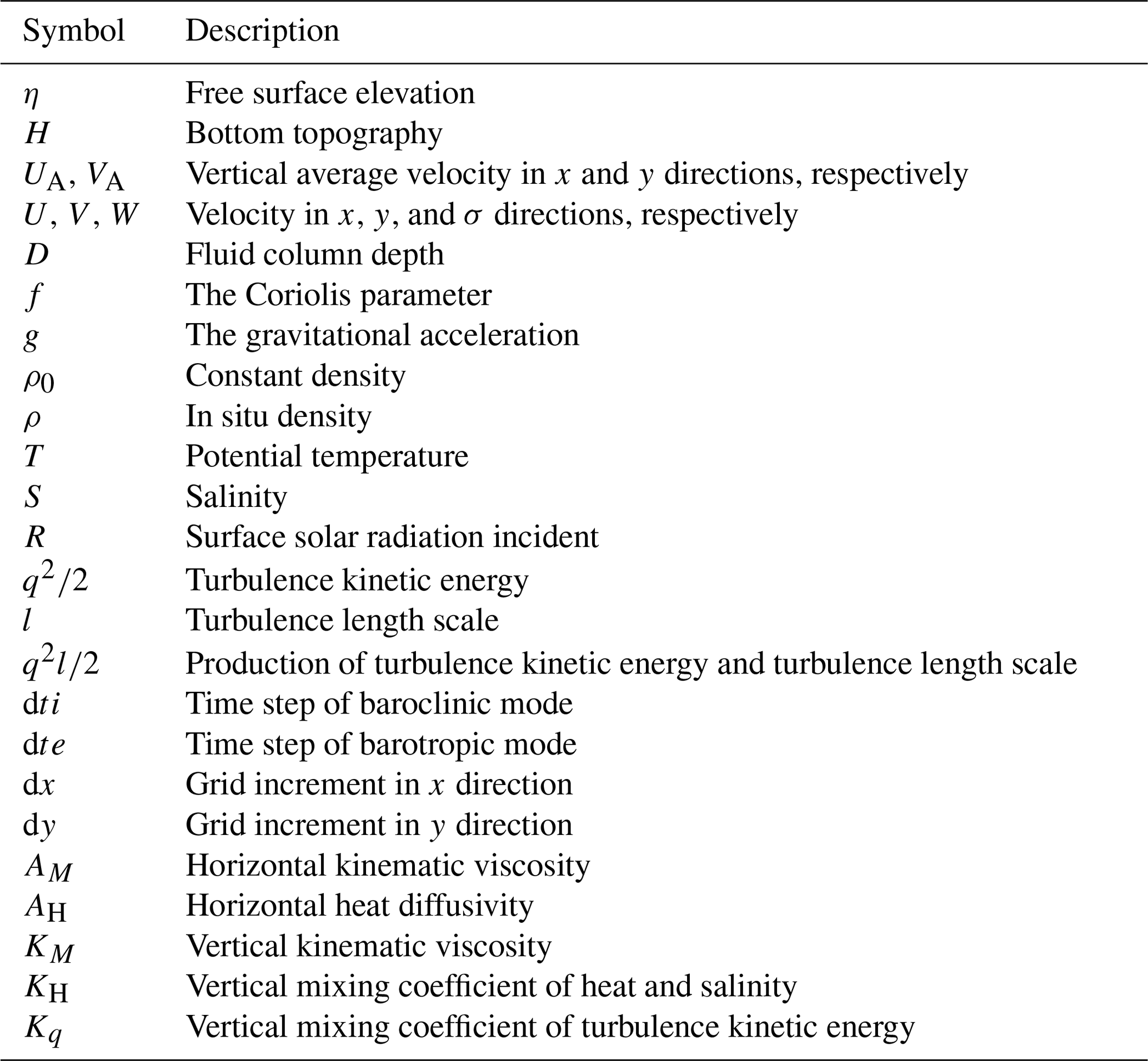
The description of each symbol in the governing equations is listed below.

Table C1Descriptions of symbols.

Download Print Version | Download XLSX

Author contributions

XiaH led the project of OpenArray and the writing of this paper. DW, QW, SZ, and XinH designed OpenArray. XinH, DW, QW, SZ, MW, YG, and QT implemented and tested GOMO. All coauthors contributed to the writing of this paper.

Competing interests

The authors declare that they have no conflict of interest.

Acknowledgements

Xiaomeng Huang is supported by a grant from the National Key R&D Program of China (2016YFB0201100), the National Natural Science Foundation of China (41776010), and the Center for High Performance Computing and System Simulation of the Pilot National Laboratory for Marine Science and Technology (Qingdao). Xing Huang is supported by a grant from the National Key R&D Program of China (2018YFB0505000). Shixun Zhang is supported by a grant from the National Key R&D Program of China (2017YFC1502200) and Qingdao National Laboratory for Marine Science and Technology (QNLM2016ORP0108). Zhenya Song is supported by National Natural Science Foundation of China (U1806205) and AoShan Talents Cultivation Excellent Scholar Program supported by Qingdao National Laboratory for Marine Science and Technology (2017ASTCP-ES04).

Financial support

This research has been supported by the National Key R&D Program of China (grant nos. 2016YFB0201100, 2018YFB0505000, and 2017YFC1502200), the National Natural Science Foundation of China (grant nos. 41776010 and U1806205), and the Qingdao National Laboratory for Marine Science and Technology (grant nos. QNLM2016ORP0108 and 2017ASTCP-ES04).

Review statement

This paper was edited by Steven Phipps and reviewed by David Webb and two anonymous referees.

References

Abadi, M., Barham, P., Chen, J., Chen, Z., Davis, A., Dean, J., Devin, M., Ghemawat, S., Irving, G., Isard, M., Kudlur, M., Levenberg, J., Monga, R., Moore, S., Murray, D. G., Steiner, B., Tucker, P., Vasudevan, V., Warden, P., Wicke, M., Yu, Y., and Zheng, X.: TensorFlow: A System for Large-Scale Machine Learning, in 12th USENIX Symposium on Operating Systems Design and Implementation (OSDI 16) USENIX Association, Savannah, GA, 265–283, available at: https://www.usenix.org/conference/osdi16/technical-sessions/presentation/abadi (last access: 28 October 2019), 2016.

Alexander, K. and Easterbrook, S. M.: The software architecture of climate models: a graphical comparison of CMIP5 and EMICAR5 configurations, Geosci. Model Dev., 8, 1221–1232, https://doi.org/10.5194/gmd-8-1221-2015, 2015.

Arakawa, A. and Lamb, V. R.: A Potential Enstrophy and Energy Conserving Scheme for the Shallow Water Equations, Mon. Weather Rev., 109, 18–36, https://doi.org/10.1175/1520-0493(1981)109<0018:APEAEC>2.0.CO;2, 1981.

Bae, H., Mustafa, D., Lee, J. W., Aurangzeb, Lin, H., Dave, C., Eigenmann, R., and Midkiff, S. P.: The Cetus source-to-source compiler infrastructure: Overview and evaluation, Int. J. Parallel Prog., 41, 753–767, 2013.

Bastien, F., Lamblin, P., Pascanu, R., Bergstra, J., Goodfellow, I. J., Bergeron, A., Bouchard, N., Warde-Farley, D., and Bengio, Y.: Theano: new features and speed improvements, CoRR, abs/1211.5, available at: http://arxiv.org/abs/1211.5590 (last access: 28 October 2019), 2012.

Beckmann, A. and Haidvogel, D. B.: Numerical simulation of flow around a tall isolated seamount, Part I: problem formulation and model accuracy, J. Phys. Oceanogr., 23, 1736–1753, https://doi.org/10.1175/1520-0485(1993)023<1736:NSOFAA>2.0.CO;2, 1993.

Bloss, A., Hudak, P., and Young, J.: Code optimizations for lazy evaluation, Lisp Symb. Comput., 1, 147–164, https://doi.org/10.1007/BF01806169, 1988.

Blumberg, A. F. and Mellor, G. L.: A description of a three dimensional coastal ocean circulation model, Coast. Est. Sci., 4, 1–16, 1987.

Bonan, G. B. and Doney, S. C.: Climate, ecosystems, and planetary futures: The challenge to predict life in Earth system models, Science, 80, 6357, https://doi.org/10.1126/science.aam8328, 2018.

Che, S., Boyer, M., Meng, J., Tarjan, D., Sheaffer, J. W., Lee, S. H., and Skadron, K.: Rodinia: A benchmark suite for heterogeneous computing, in: Proceedings of the 2009 IEEE International Symposium on Workload Characterization, IISWC 2009, 2009.

Chen, C., Liu, H., and Beardsley, R. C.: An unstructured grid, finite-volume, three-dimensional, primitive equations ocean model: Application to coastal ocean and estuaries, J. Atmos. Ocean. Tech., 20, 159–186, https://doi.org/10.1175/1520-0426(2003)020<0159:AUGFVT>2.0.CO;2, 2003.

Collins, M., Minobe, S., Barreiro, M., Bordoni, S., Kaspi, Y., Kuwano-Yoshida, A., Keenlyside, N., Manzini, E., O'Reilly, C. H., Sutton, R., Xie, S. P., and Zolina, O.: Challenges and opportunities for improved understanding of regional climate dynamics, Nat. Clim. Change, 8, 101–108, https://doi.org/10.1038/s41558-017-0059-8, 2018.

Corliss, G. and Griewank, A.: Operator Overloading as an Enabling Technology for Automatic Differentiation, preprint MCS-P358–0493, Argonne National Laboratory, available at: https://pdfs.semanticscholar.org/77f8/2be571558246e564505cc654367bf38977e1.pdf (last access: 28 October 2019), 1993.

Deconinck, W., Bauer, P., Diamantakis, M., Hamrud, M., Kühnlein, C., Maciel, P., Mengaldo, G., Quintino, T., Raoult, B., Smolarkiewicz, P. K., and Wedi, N. P.: Atlas?: A library for numerical weather prediction and climate modelling, Comput. Phys. Commun., 220, 188–204, https://doi.org/10.1016/j.cpc.2017.07.006, 2017.

Dennis, J. M.: Inverse space-filling curve partitioning of a global ocean model, Proc. – 21st Int. Parallel Distrib. Process. Symp. IPDPS 2007, Abstr. CD-ROM, 1–10, https://doi.org/10.1109/IPDPS.2007.370215, 2007.

Frigo, M. and Strumpen, V.: Cache oblivious stencil computations, in: Proceeding ICS '05 Proceedings of the 19th annual international conference on Supercomputing, 361–366, https://doi.org/10.1145/1088149.1088197, 2005.

Fu, H., He, C., Chen, B., Yin, Z., Zhang, Z., Zhang, W., Zhang, T., Xue, W., Liu, W., Yin, W., Yang, G., and Chen, X.: 18.9-Pflops nonlinear earthquake simulation on Sunway TaihuLight: enabling depiction of 18-Hz and 8-meter scenarios, in: Proceedings of the International Conference for High Performance Computing, Networking, Storage and Analysis, 2017.

Griffies, S. M., Böning, C., Bryan, F. O., Chassignet, E. P., Gerdes, R., Hasumi, H., Hirst, A., Treguier, A.-M., and Webb, D.: Developments in ocean climate modelling, Ocean Model., 2, 123–192, https://doi.org/10.1016/S1463-5003(00)00014-7, 2000.

Gysi, T., Osuna, C., Fuhrer, O., Bianco, M., and Schulthess, T. C.: STELLA: A Domain-specific Tool for Structured Grid Methods in Weather and Climate Models, Proc. Int. Conf. High Perform. Comput. Networking, Storage Anal. – SC '15, 1–12, https://doi.org/10.1145/2807591.2807627, 2015.

Huang, W., Ghosh, S., Velusamy, S., Sankaranarayanan, K., Skadron, K. and Stan, M. R.: HotSpot: A compact thermal modeling methodology for early-stage VLSI design, IEEE T. VLSI Syst., 14, 501–513, https://doi.org/10.1109/TVLSI.2006.876103, 2006.

Huang, X. M., Wang, W. C., Fu, H. H., Yang, G. W., Wang, B., and Zhang, C.: A fast input/output library for high-resolution climate models, Geosci. Model Dev., 7, 93–103, https://doi.org/10.5194/gmd-7-93-2014, 2014.

Huang, X., Wu, Q., Wang, D., Huang, X., and Zhang, S.: OpenArray, available at: https://github.com/hxmhuang/OpenArray, last access: 28 October 2019a.

Huang, X., Huang, X., Wang, D., Wu, Q., Zhang, S. and Li, Y.: A simple user manual for OpenArray version 1.0, available at: https://github.com/hxmhuang/OpenArray/tree/master/doc, last access: 28 October 2019b.

Huang, X., Huang, X., Wang, M., Wang, D., Wu, Q., and Zhang, S.: GOMO, available at: https://github.com/hxmhuang/GOMO, last access: 28 October 2019c.

Korn, P.: Formulation of an unstructured grid model for global ocean dynamics, J. Comput. Phys., 339, 525–552, https://doi.org/10.1016/j.jcp.2017.03.009, 2017.

Lawrence, B. N., Rezny, M., Budich, R., Bauer, P., Behrens, J., Carter, M., Deconinck, W., Ford, R., Maynard, C., Mullerworth, S., Osuna, C., Porter, A., Serradell, K., Valcke, S., Wedi, N., and Wilson, S.: Crossing the chasm: how to develop weather and climate models for next generation computers?, Geosci. Model Dev., 11, 1799–1821, https://doi.org/10.5194/gmd-11-1799-2018, 2018.

Levin, J. G., Iskandarani, M., and Haidvogel, D. B.: A nonconforming spectral element ocean model, Int. J. Numer. Meth. Fl., 34, 495–525, https://doi.org/10.1002/1097-0363(20001130)34:6<495::AID-FLD68>3.0.CO;2-K, 2000.

Lidman, J., Quinlan, D. J., Liao, C., and McKee, S. A.: ROSE::FTTransform β-A source-to-source translation framework for exascale fault-tolerance research, Proc. Int. Conf. Dependable Syst. Networks, https://doi.org/10.1109/DSNW.2012.6264672, 25–28 June 2012.

Mellor, G. L. and Yamada, T.: Development of a turbulence closure model for geophysical fluid problems, Rev. Geophys., 20, 851–875, https://doi.org/10.1029/RG020i004p00851, 1982.

Mellor-Crummey, J., Adhianto, L., Scherer III, W. N., and Jin, G.: A New Vision for Coarray Fortran, in Proceedings of the Third Conference on Partitioned Global Address Space Programing Models, ACM, New York, NY, USA, 5:1–5:9, 2009.

National Research Council: A National Strategy for Advancing Climate Modeling, National Academies Press, Washington, D.C., https://doi.org/10.17226/13430, 2012.

Porkoláb, Z., Mihalicza, J., and Sipos, Á.: Debugging C $+ +$ template metaprograms, in: Proceeding GPCE '06 Proceedings of the 5th international conference on Generative programming and component engineering, 255–264, https://doi.org/10.1145/1173706.1173746, 2007.

Pugh, W.: Uniform Techniques for Loop Optimization, in Proceedings of the 5th International Conference on Supercomputing, ACM, New York, NY, USA, 341–352, 1991.

Qiao, F., Zhao, W., Yin, X., Huang, X., Liu, X., Shu, Q., Wang, G., Song, Z., Li, X., Liu, H., Yang, G., and Yuan, Y.: A Highly Effective Global Surface Wave Numerical Simulation with Ultra-High Resolution, in: International Conference for High Performance Computing, Networking, Storage and Analysis, SC, 2017.

Reynolds, J. C.: Theories of Programming Languages, Cambridge University Press, New York, NY, USA, 1999.

Shan, A.: Heterogeneous Processing: A Strategy for Augmenting Moore's Law, Linux J., 142, available at: http://dl.acm.org/citation.cfm?id=1119128.1119135 (last access: 28 October 2019), 2006.

Shchepetkin, A. F. and McWilliams, J. C.: The regional oceanic modeling system (ROMS): A split-explicit, free-surface, topography-following-coordinate oceanic model, Ocean Model., 9, 347–404, https://doi.org/10.1016/j.ocemod.2004.08.002, 2005.

Suganuma, T. and Yasue, T.: Design and evaluation of dynamic optimizations for a Java just-in-time compiler, ACM Trans., 27, 732–785, https://doi.org/10.1145/1075382.1075386, 2005.

Taylor, K. E., Stouffer, R. J., and Meehl, G. A.: An overview of CMIP5 and the experiment design, B. Am. Meteorol. Soc., 93, 485–498, https://doi.org/10.1175/BAMS-D-11-00094.1, 2012.

Torres, R., Linardakis, L., Kunkel, J., and Ludwig, T.: ICON DSL: A Domain-Specific Language for climate modeling, In: International Conference for High Performance Computing, Networking, Storage and Analysis, available at: http://sc13.supercomputing.org/sites/default/files/WorkshopsArchive/pdfs/wp127s1.pdf (last access: 28 October 2019), 2013.

van Engelen, R. A.: ATMOL: A Domain-Specific Language for Atmospheric Modeling, J. Comput. Inf. Technol., 9, 289–303, https://doi.org/10.2498/cit.2001.04.02, 2001.

Walther, A., Griewank, A., and Vogel, O.: ADOL-C: Automatic Differentiation Using Operator Overloading in C $+ +$ , PAMM, https://doi.org/10.1002/pamm.200310011, 2003.

Xu, S., Huang, X., Oey, L.-Y., Xu, F., Fu, H., Zhang, Y., and Yang, G.: POM.gpu-v1.0: a GPU-based Princeton Ocean Model, Geosci. Model Dev., 8, 2815–2827, https://doi.org/10.5194/gmd-8-2815-2015, 2015.

Articles

Short summary

We designed a simple computing library (OpenArray) to decouple ocean modelling and parallel computing. OpenArray provides 12 basic operators featuring user-friendly interfaces and an implicit parallelization ability. Based on OpenArray, we implement a practical ocean model with an enhanced readability and an excellent scalable performance. OpenArray may signal the beginning of a new frontier in future ocean modelling through ingesting basic operators and cutting-edge computing techniques.