the Creative Commons Attribution 4.0 License.
the Creative Commons Attribution 4.0 License.
 | 26 Feb 2024
Long-term monitoring (1953–2019) of geomorphologically active sections of Little Ice Age lateral moraines in the context of changing meteorological conditions
Madlene Pfeiffer
Florian Haas
Jakob Rom
Fabian Fleischer
Tobias Heckmann
Livia Piermattei
Michael Wimmer
Lukas Braun
Manuel Stark
Sarah Betz-Nutz
Michael Becht
We show a long-term erosion monitoring of several geomorphologically active gully systems on Little Ice Age lateral moraines in the European Central–Eastern Alps, covering a total time period from 1953 to 2019 and including several survey periods in order to identify corresponding morphodynamic trends. For the implementation, DEM (digital elevation model) of Differences (DoDs) were calculated, based on multitemporal high-resolution digital elevation models from historical aerial images (generated by structure from motion photogrammetry with multi-view stereo) and light detection and ranging from airborne platforms. Two approaches were implemented to achieve the corresponding objectives. First, by calculating linear regression models using the accumulated sediment yield and the corresponding catchment area (on a log–log scale), the range of the variability in the spatial distribution of erosion values within the sites. Second, we use volume calculations to determine the total and the mean sediment yield (as well as erosion rates) of the entire sites. Subsequently, both the sites and the different time periods of both approaches are compared. Based on the slopes of the calculated regression lines, it can be shown that the highest variability in the sediment yield at the sites occurs in the first time period (mainly 1950s to 1970s). This can be attributed to the fact that within some sites the sediment yield per square metre increases clearly more strongly (regression lines with slopes up to 1.5). In contrast, in the later time periods (1970s to mid-2000s and mid-2000s to 2017/2019), there is generally a decrease in 10 out of 12 cases (regression lines with slopes around 1). However, even at sites with an increase in the variability in the sediment yield over time, the earlier high variabilities are no longer reached. This means that the spatial pattern of erosion in the gully heads changes over time as it becomes more uniform. Furthermore, using sediment volume calculations and corresponding erosion rates, we show a generally decreasing trend in geomorphic activity (amount of sediment yield) between the different time periods in 10 out of 12 sites, while 2 sites show an opposite trend, where morphodynamics increase and remain at the same level. Finally, we summarise the results of long-term changes in the morphodynamics of geomorphologically active areas on lateral moraines by presenting the “sediment activity concept”, which, in contrast to theoretical models, is based on actually calculated erosion. The level of geomorphic activity depends strongly on the characteristics of the sites, such as size, slope length, and slope gradient, some of which are associated with deeply incised gullies. It is noticeable that especially areas with influence of dead ice over decades in the lower slope area show high geomorphic activity. Furthermore, we show that system internal factors, as well as the general paraglacial adjustment process, have a greater influence on long-term morphodynamics than changing external weather and climate conditions, which, however, had a slight impact mainly in the last, i.e. most recent, time period (mid-2000s to 2017/2019) and may have led to an increase in erosion at the sites.
- Article
(18359 KB) - Full-text XML
- BibTeX
- EndNote


Since the end of the Little Ice Age (LIA) around 1850 (Matthews and Briffa, 2005; Ivy-Ochs et al., 2009) and the strong global warming of the last few decades (IPCC, 2021; Pepin et al., 2022), proglacial areas have played a special role in the current landscape changes in the high-alpine geosystems, as such areas are strongly extending due to the ongoing retreat of the glaciers (Deline et al., 2015; Heckmann and Morche, 2019; Haeberli and Whiteman, 2021). The melting of glaciers leads to the release of unstable sediment sources, which are subsequently exposed to several geomorphological slope processes, which can lead to high erosion rates.
The relationship between this glacier melt and slope instability has been subject of research for several decades. Church and Ryder (1972) were the first to develop a theoretical model (“paraglacial concept”) to describe future landscape change throughout a proglacial area and defined the phase of transition as the paraglacial period, which is the period during which paraglacial processes (non-glacial processes) occur. After a period of high geomorphic activity (fluvial erosion and transport) associated with a peak, sediment production decreases over time until a “normal” level of sediment movement is reached. By further developing the model, Ballantyne (2002a) describes this paraglacial landscape adjustment using the “sediment exhaustion model”, which is based on a hypothetical paraglacial system. Several variable factors determine the duration of this period, such as sediment release and the rate of sediment reworking. Following the sediment exhaustion model, the rate of sediment reworking of glaciogenic sediments in proglacial areas decreases exponentially if the sediment release rate only depends on sediment availability (Ballantyne, 2002a, b).
Ballantyne and Benn (1994) and Curry (1999) describe the paraglacial slope adjustment of lateral moraines by analysing the formation of gully systems on lateral moraines and the corresponding alluvial fans and debris cones (both in western Norway). These systems result from weathering and erosion, such as fluvial erosion, slope wash, debris flows, smaller slope failures, and earth or snow avalanches (Ballantyne, 2002a, b; Curry et al., 2006; Haas et al., 2012; Dusik et al., 2019). Material is deposited in the gullies (e.g. by nival processes, fluvial activity, and sidewall collapse) and subsequently transported downslope, mainly by debris flows triggered in the gully heads after heavy rainfall or after rapid snowmelt (Ballantyne and Benn, 1994; Ballantyne, 2002b; Curry et al., 2006). Similarly, large deformations such as deep-seated slope failures and landslides with low frequency and high magnitude also occur (Mattson and Gardner, 1991; Blair, 1994; Hugenholtz et al., 2008; Altmann et al., 2020; Cody et al., 2020; Betz-Nutz, 2021; Zhong et al., 2022). These erosion processes are primarily driven by temperature and precipitation events, which have been subject to change in recent years and decades (Serquet et al., 2011; Brugnara et al., 2012; Mankin and Diffenbaugh, 2015; Klein et al., 2016; Beniston et al., 2018; Hock et al., 2019; IPCC, 2021; Pepin et al., 2022). Springtime snowmelt provides important preparatory steps for sediment transport processes, such as loosening of the upper layers of sediments of the slope or through the delivery of material into the gullies by nival processes, which is then transported downslope by debris flows in the summer months (Haas et al., 2012; Dusik et al., 2019), which is considered to be the most important process occurring (Ballantyne, 2002a; Curry et al., 2006). Dusik (2019) also shows a positive correlation between the number of mass movements, the number of extreme precipitation intensities, and the number of certain threshold exceedances for extreme daily precipitation totals, as well as annual precipitation totals. These processes ultimately lead to the dissection of the upper parts of the lateral moraines, which is, however, limited in time (Curry et al., 2006). Curry et al. (2009) inferred from morphometric measurements along a chronosequence that gullies increase in depth, width, area, and volume over time, with width increasing significantly more than depth, resulting in the older ones not being as densely gullied. Furthermore, it is described that the slope gradient decreases over time; for example, Ballantyne and Benn (1994) report an average of 5° (in 48 years between 1943 and 1991). Betz-Nutz et al. (2023) document a range of slope gradient changes between −3.2 and +6.6° between the ∼ 1950s and 2018 (∼ 68 years), showing that both increases and decreases can occur. Ballantyne and Benn (1994), Curry (1999), and Curry et al. (2006) give average annual erosion rates of different gully systems over several decades estimated by the volume of the gullies. Curry et al. (2006) showed at different test sites in the Swiss Alps that the maximum extent of gullies is reached after 50 years of ice release and that sediment filling and stabilisation occurs after 80–140 years of deglaciation. While 50 % of the available sediment is exhausted after 10–50 years, it can take several centuries until the paraglacial adjustment process is completed (Curry et al., 2006). Schiefer and Gilbert (2007) show, based on quantitative analyses (via stereophotogrammetry using historical aerial images), a significant decrease in the geomorphic activity of gully systems on lateral moraines over several decades and different time periods in the glacier foreland of the Lillooet Glacier (British Columbia, Canada). Carrivick et al. (2013) generally confirm the concept of paraglacial adjustment by showing decreasing morphodynamics with increasing distance from the glacier, as they have been ice-free for a longer time. However, the lower morphodynamics observed in the distal areas of the glacier forelands could also be due to the generally lower slope gradients there (Betz-Nutz et al., 2023). Lane et al. (2017) showed, in the glacier foreland of Arolla Glacier (Valais, Switzerland), that there are no indications of filling in the developed gully systems, which indicates that they are still in the incision phase. Betz-Nutz et al. (2023) show, with the use of historical aerial photographs (processed by structure from motion (SfM) photogrammetry), that the paraglacial adjustment process over decades is very variable. While 13 out of 20 moraine sections showed decreasing erosion rates over decades, divided into several time periods, six showed almost constant activity, and one section even showed a substantial increase in erosion rate.
The period of paraglacial landscape adjustment is also influenced by upcoming vegetation, which can be considered both a consequence and a cause of slope stabilisation (Eichel et al., 2016, 2023; Haselberger et al., 2021, 2022). Nevertheless, bound solifluction processes can occur under a dense vegetation cover and are therefore not an absolute sign of stabilisation (Draebing and Eichel, 2017).
The generation of multitemporal accurate and precise digital elevation models (DEMs) and the resulting DEM of Differences (DoDs) by different remote sensing methods and techniques, which have been established in geomorphological research in recent years, enabled the detection of changes in the Earth's surface in high spatial and temporal resolution (Pulighe and Fava, 2013; Nebiker et al., 2014; Tarolli, 2014; Smith et al., 2016; Eltner et al., 2016; Sevara et al., 2018; Okyay et al., 2019; Noto et al., 2017). By processing overlapping high-resolution digitised historical aerial images of high-alpine geosystems, using SfM–MVS (structure from motion with multi-view stereo) digital stereophotogrammetry in combination with current airborne lidar (light detection and ranging) data into DEMs and the corresponding DoDs, landscape changes in these areas can be reconstructed over several decades (Midgley and Tonkin, 2017; Mölg and Bolch, 2017; Lane et al., 2017; Betz et al., 2019; Altmann et al., 2020; Fleischer et al., 2021; Betz-Nutz, 2021; Stark et al., 2022; Piermattei et al., 2023). The spatial distribution of positive and negative DoD elevation changes enable various analyses, such as the reconstruction and interpretation of individual geomorphological processes (Dusik, 2019) or the calculation of morphological budgets (Altmann et al., 2020).
Furthermore, by applying flow-routing algorithms and the accumulation of DoD values accordingly, sediment yield from the contributing area of each cell can be determined. Pelletier and Orem (2014) used repeat airborne lidar-based DEMs before and after a wildfire and calculated for each pixel the net sediment volume exported by geomorphological processes. Further applications of this methodology have been published by Wester et al. (2014), who calculated the total sediment yield by applying a weighted flow accumulation algorithm, and Heckmann and Vericat (2018), who further developed the approach by calculating a spatially distributed measure of functional sediment connectivity on a proglacial slope. Neugirg et al. (2015a, b, 2016) showed a positive correlation between log sediment yield (calculated by accumulated DoD values on slopes) and the corresponding log sediment-contributing area, respectively, log catchment area (using the sediment-contributing-area approach), both extracted at randomly selected cells of the channel network (so-called “virtual sediment traps”). Alongside these studies conducted over several months and years on slopes in the Northern Alps (Lainbach valley and Arzbach valley, Germany) and at a former iron ore mine on the island of Elba in the Tyrrhenian Sea (next to Rio Marina, Italy), this approach was also applied by Dusik (2019) and Dusik et al. (2019) over several weeks to a proglacial slope in Kaunertal (Tyrol, Austria). One advantage of this approach is that it can be used to determine not only the size of the sediment yield (which can be compared with previous time periods, for example) but also the variability in the sediment yield within the site in a time period (spatial pattern of sediment yield within the site), which is not possible, for example, when calculating simple erosion rates, where only the volume of the total change can be computed.
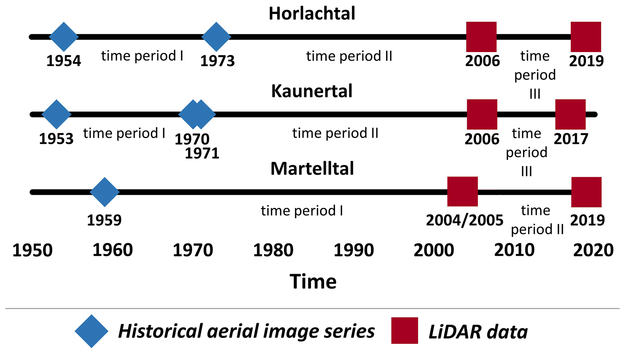
In this study we apply the sediment-contribution-area approach to several LIA lateral moraine sections over several decades and several time periods in the European Central–Eastern Alps in order to better understand the paraglacial adjustment process of lateral moraines. Thus, the aim is to find out how the spatial erosion pattern within the areas changes over time. Second, we show volume calculations of the entire sites to determine the total sediment yield (and erosion rates). Therefore, by combining high-resolution historical and current DEMs and the corresponding DoDs, we show quantification and analysis of gully system morphodynamics at 12 different sections in the upper reaches of lateral moraines in five different glacier forelands over a total period of several decades (1953–2019) with several survey periods (∼ 1950s to ∼ 1970s, ∼ 1970s to ∼ 2000s, and ∼ 2000s to 2017/2019). Using simulated climate data of the glacier forelands, we were also able to investigate, besides system internal influences, external impacts on the morphodynamics, which have not been considered in long-term studies on erosion of the LIA lateral moraines so far.
The sites are located in different high-alpine geosystems along a north–south axis in the European Central–Eastern Alps and are situated north (Horlachtal and upper Kaunertal) and south (upper Martelltal) of the main Alpine divide. In these valleys, the sites are located within five glacier forelands on lateral moraines formed by the glaciers during their maximum glacier outline during the LIA around 1850 (Fig. 1). The Horlachtal is located in the Stubai Alps (Tyrol, Austria), which is a tributary of the Oetztal (Geitner, 1999; Rieger, 1999). The investigated section of the Horlachtal is located in the side valley and sub-catchment Grastal (glacier foreland Grastalferner), which is oriented in a north–south direction. Geologically, the Horlachtal is located in the Oetztal Massif, where gneisses and mica schists dominate (Becht, 1995; Geitner, 1999). The Kaunertal is also located in the Oetztal Alps (Tyrol, Austria) and is oriented in a north–south direction. This valley geologically belongs to the Austroalpine crystalline complex (Tollmann, 1977; Geological Survey of Austria, 1999), where crystalline rocks, mainly ortho- and paragneisses, dominate (Vehling, 2016). The sites within the Kaunertal are located in the glacier forelands of the Gepatschferner, another glacier outlet of the Gepatschferner, the so-called Münchner Abfahrt (MA), and the Weißseeferner. The Martelltal is a southwest–northeast oriented valley located in the Ortler–Cevedale group (southern Tyrol, Italy) and belongs geologically to the Ortler–Campo crystalline, where quartz phyllite dominates, with layers of, for example, shales, gneisses, and marbles (Mair and Purtscheller, 1996; Staindl, 2000; Mair et al., 2007). The two sites are located in the glacier foreland of the Hohenferner. All valleys are characterised by the continental climate and low annual precipitation sums of the inner alpine dry region (Becht, 1995; Hagg and Becht, 2000; Veit, 2002; Hilger, 2017; Betz-Nutz, 2021). The sites are characterised by very sparse vegetation cover, intense paraglacial morphodynamics, and typical unsorted moraine material. Table 1 and Fig. 1 give an overview of the location, as well as the characteristics of the sites.
Table 1Characteristics of the sites. Values were derived from 2017 DEM (Kaunertal) and 2019 DEM (Horlachtal and Martelltal).
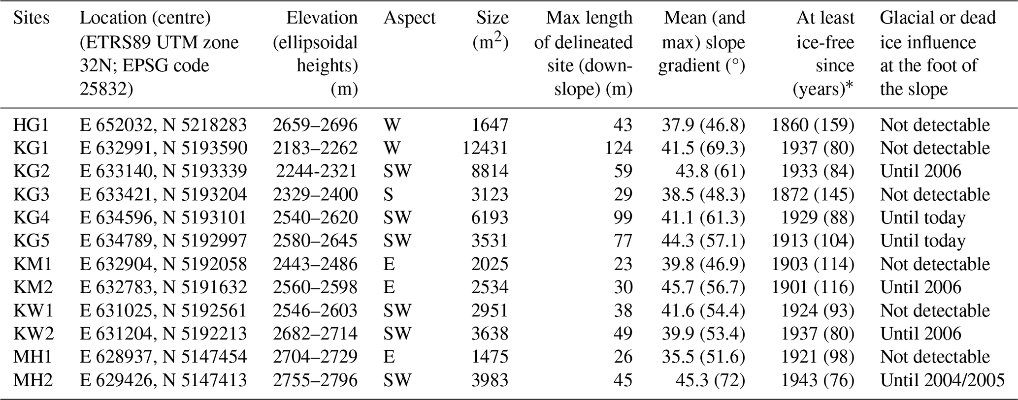
*Determination of complete deglacialisation is based on an interpolation between the two glacier outlines within which the sites have become ice-free by calculating the Euclidean distance, as proposed by Betz-Nutz et al. (2023).
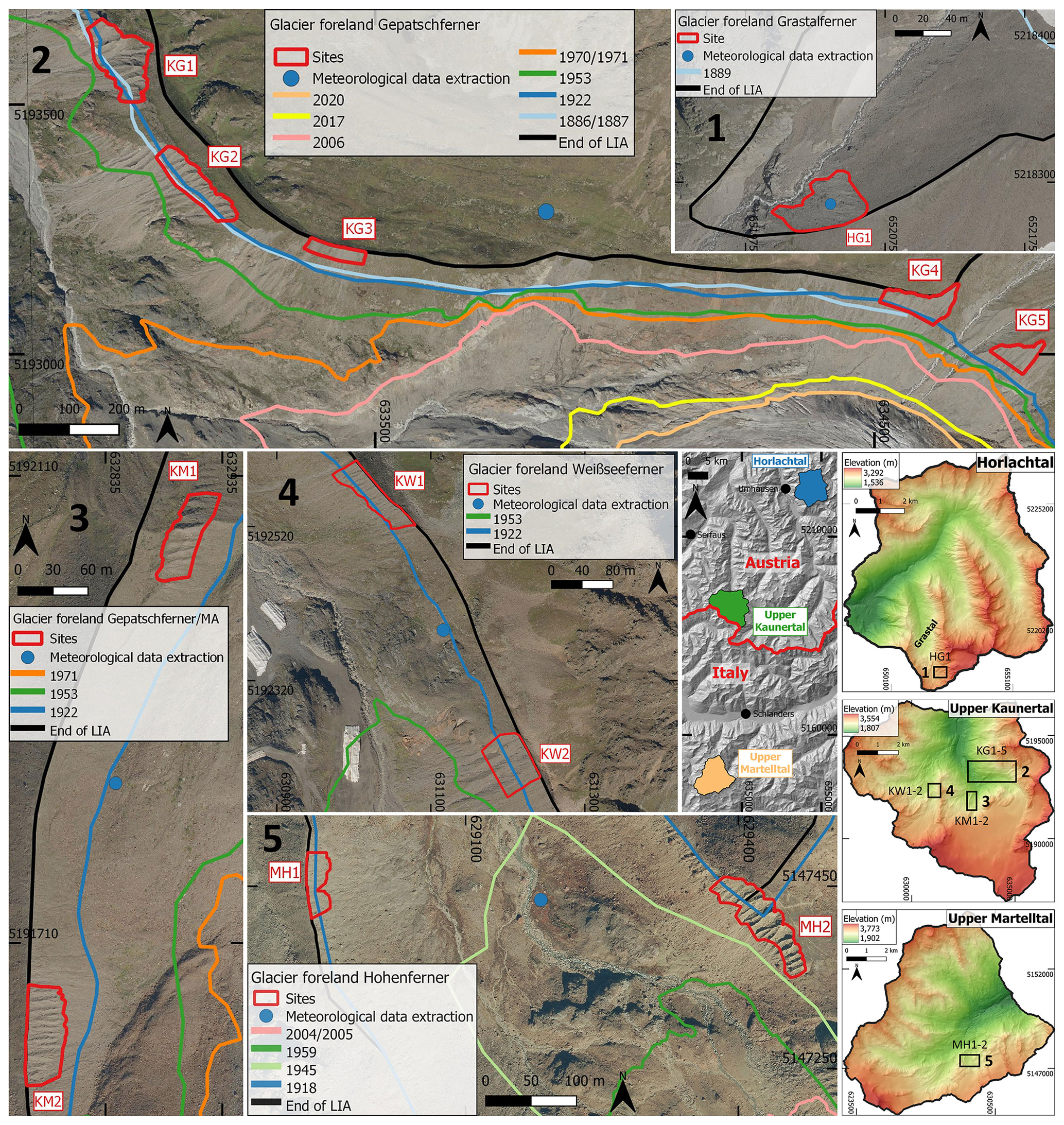
Figure 1Location of the sites, glacier outlines (sources in Table 2), and location for meteorological data extraction (for corresponding analysis, see Sect. 3.3). Large-scale elevation data (digital surface model, DSM, 25 m) (centre right) are based on the Shuttle Radar Topography Mission (SRTM), and the Terra Advanced Spaceborne Thermal Emission and Reflection Radiometer (ASTER) Global Digital Elevation Model (GDEM) (Copernicus, 2016). DEMs (1 m) (right and bottom right) are based on airborne lidar (airborne laser scanning, ALS) data from 2017 (Kaunertal) and 2019 (Horlachtal and Martelltal) (see Sect. 3.1.1). Orthophotos (from 2020) are provided by the province of Tyrol (Horlachtal and Kaunertal) and by the Autonomous Province of Bolzano, southern Tyrol (Martelltal). The glacier outline of Groß and Patzelt (2015) is based on mapping of the LIA lateral moraines and field surveys based on orthophotos. In the process of this study, these mappings were slightly modified so that they fit to the maximum glacier outline (LIA lateral moraines) more accurately. The glacier outlines end of the LIA, 1918, 1945, and 1959 in the Martelltal have already been described by Betz et al. (2019).
Table 2Sources of the glacier outlines.
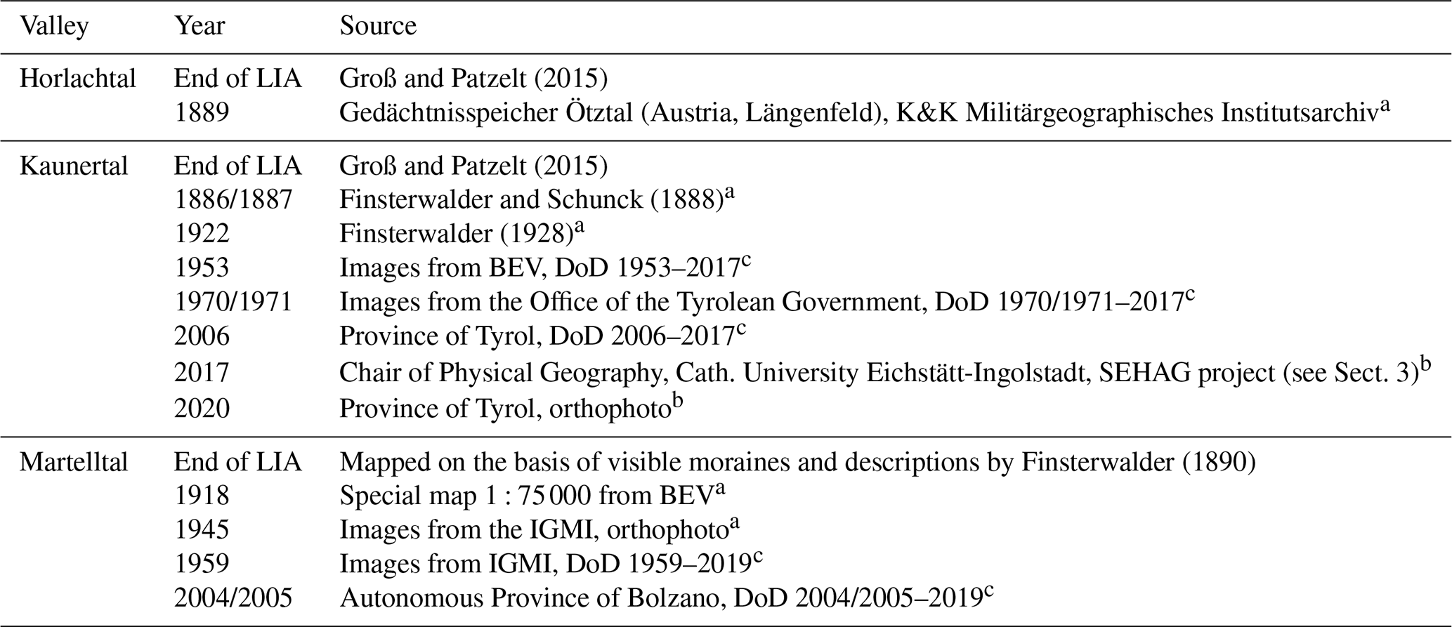
aBased on historical map. bBased on orthophoto and/or hillshade. cBased on DoD (SfM–MVS photogrammetry and/or airborne laser scanning (ALS)). Note: IGMI is the Italian Military Geographic Institute; BEV is the Federal Office of Metrology and Surveying (Vienna, Austria).
3.1 Generation of the topographic data
3.1.1 Processing of airborne lidar and photogrammetric SfM–MVS point clouds
Several data sets were used for the reconstruction of the terrain surface for the entire catchment area. These include both current airborne lidar data and historical aerial image series (Fig. 2). Thus, the time periods are based on the availability and quality of the data.
To determine the recent morphodynamics at the respective sites, available airborne lidar data from 2004/2005 to 2019 were used. The 2004/2005 and 2006 data of the three valleys were provided by the Autonomous Province of Bolzano and the province of Tyrol (Table 3). The latest airborne laser scanning (ALS) data sets of each valley (2017 and 2019) were collected in the ALS flight campaigns of the Chair of Physical Geography at the Catholic University of Eichstätt-Ingolstadt (Table 3) (Stark et al., 2022). In this case, lidar data sets were collected using previously determined flight strips. Direct georeferencing (position and altitude) of the trajectories was determined by Global Navigation Satellite System (GNSS) rover antenna and an inertial measurement unit (IMU) (Applanix AP 20), both located in the laser scanner. In addition, GNSS correction data were acquired on the ground during the flight missions using a dGNSS antenna (Fig. 3).
Table 3ALS and DEM data and corresponding flight mission attributes. NA: not available.
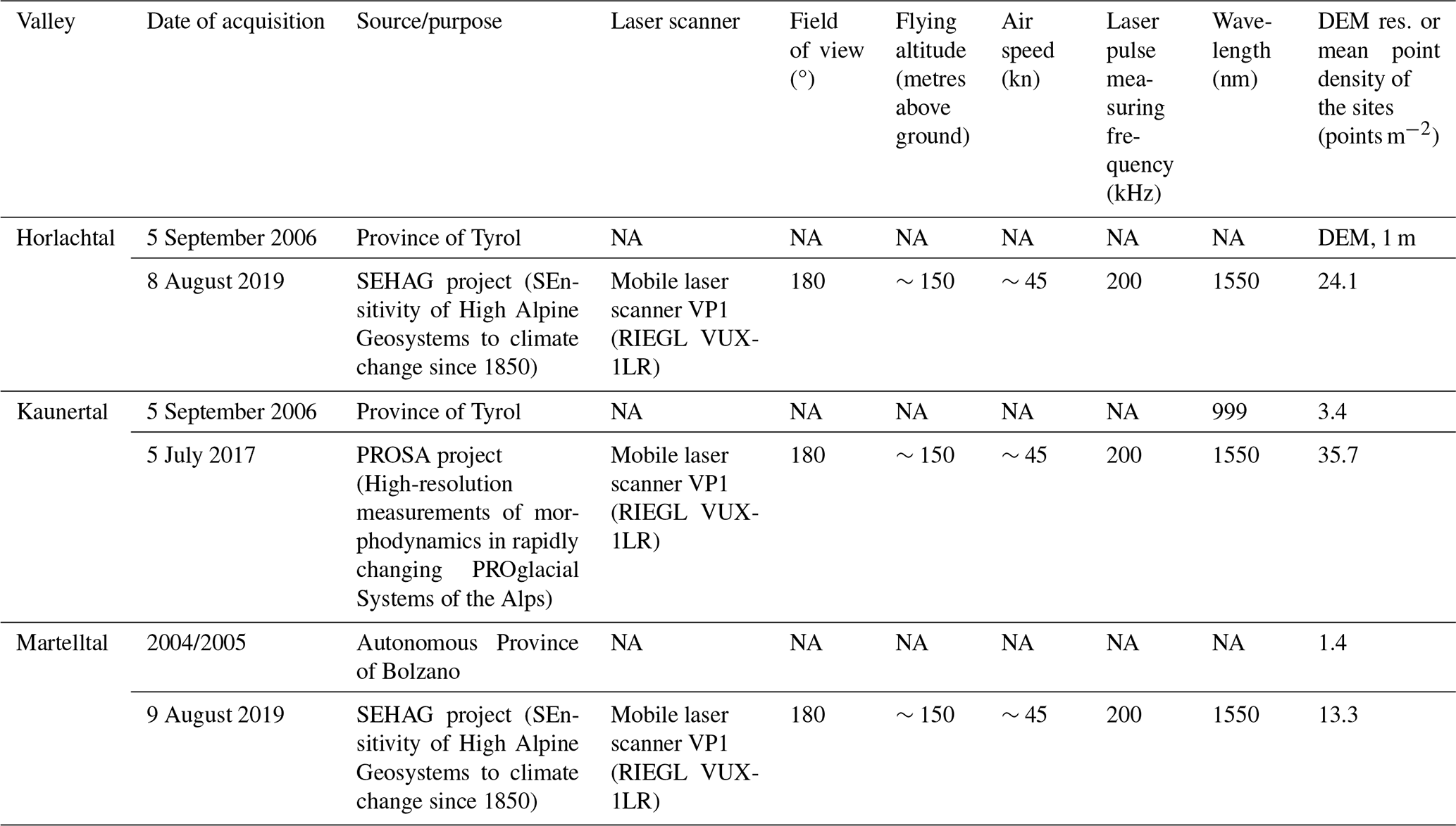
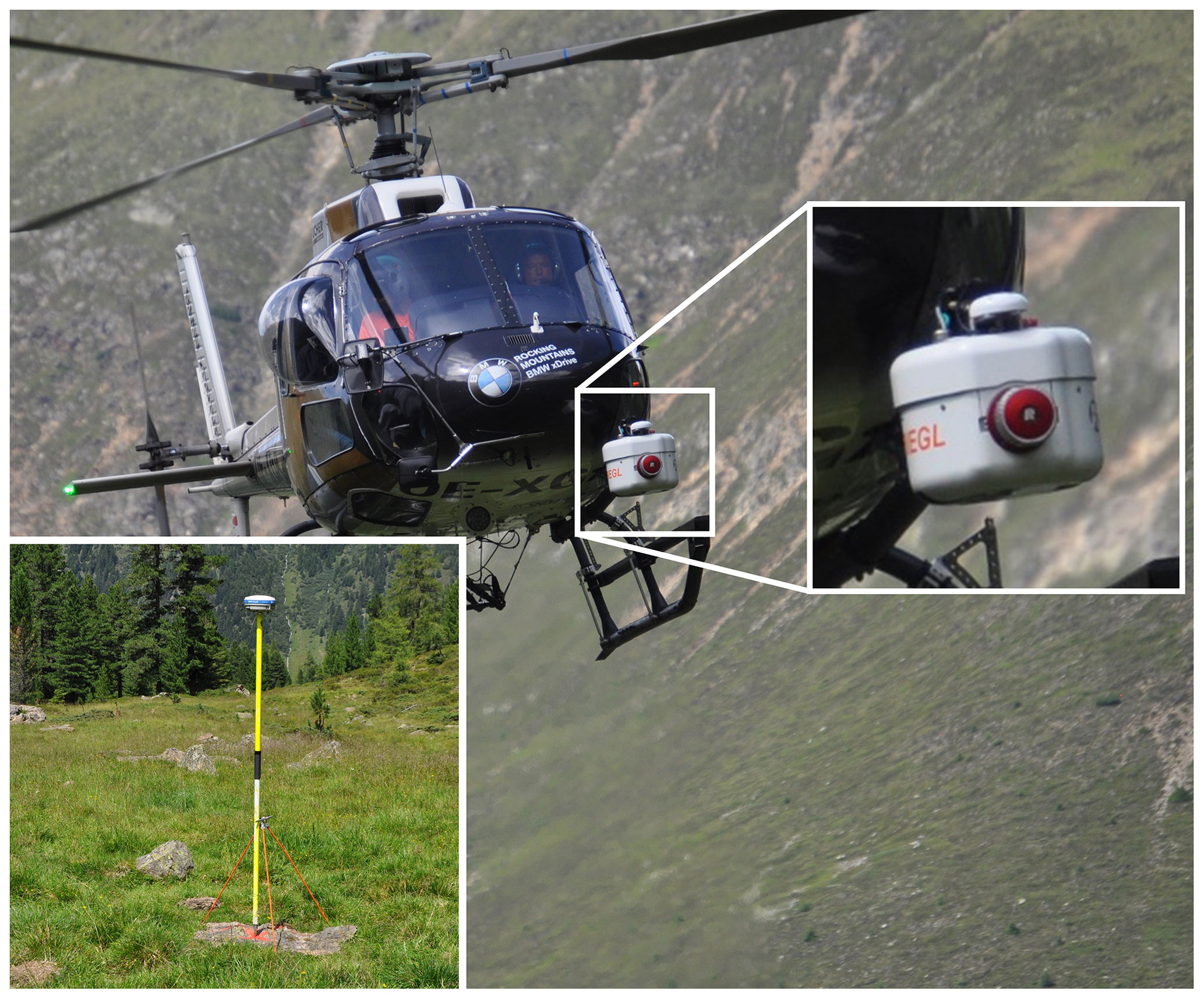
Figure 3ALS data collection on 8 August 2019 in Horlachtal. Helicopter with nose-mounted VP1 laser scanner, as well as the ground station, which recorded the dGNSS raw data during the flight time (Stonex S9III).
In order to extend the temporal scope of this study by several decades (until 1953), previously digitised (high-resolution) overlapping historical aerial images were processed into historical DEMs. Except for the 1959 Martelltal survey, camera distortion parameters and focal lengths were provided for all data with the respective camera calibration certificates (Table 4).
The digitised image series were processed with the Agisoft Metashape Professional Edition software package (Version 1.6.6; Agisoft), using structure-from-motion (SfM) photogrammetry with multi-view stereo (MVS) algorithms to generate high-resolution point clouds. The generation of point clouds from digitised historical (aerial) image series requires different preparation and processing steps. First, all images of each series were resized to a common image size (uniform number of pixels along the x and y axes) without changing the image content. This step was necessary so that the software can assign all images to the same camera (source) and was carried out using Adobe Photoshop (CS6). This is of enormous importance in order to be able to use the appropriate distortion parameters for the respective camera models for the calculation. Thereafter, the image sets were imported into single folders, and a common global coordinate system (ETRS89 UTM zone 32N; EPSG code 25832) was defined. Next, all images were masked to exclude the black edges or the frame (instrument stripes with the camera metadata) in order to avoid interference with the orientation of the cameras (Gomez et al., 2015). Before the initial processing of images, we defined the fiducial mark information and lens distortion parameters in order to set the metric dimension of images and lenses. This information was included and used for the alignment of single images (SfM).
Since a global exterior orientation requires a large number of precisely surveyed ground control points (GCPs) distributed throughout the area, we used highly precise ALS data sets with millimetre accuracy (2019 Horlachtal; 2017 Kaunertal) to extract these GCPs and to define the exterior orientation of all data. The selection and extraction of GCPs was based on clearly identifiable objects (e.g. rock formations) that were also considered to be stable (geomorphologically unchanged) over the entire observation period. If a calibration certificate was available, the film camera option was used, fiducial marks defined, and the focal length set and fixed. All other lens distortion parameters (Cx, Cy, k1, k1, k1, p1, and p2) were estimated and adjusted fully automatic using the auto-calibration function. In case of missing camera calibration certificate, an auto-calibration (no film camera) was performed. Both options were proposed by Stark et al. (2022).
According to these pre-processing steps, the point clouds were generated by the (i) initial joint orientation of the images; (ii) selection of ground control points (GCPs); (iii) final camera orientation (bundle block adjustment) including scale definition; and (iv) calculation of dense point clouds.
The processing of the 1959 point cloud, which was used in this study, is already described in Betz et al. (2019).
Table 4Overview of acquired historical image series for point cloud generation and corresponding DEMs by photogrammetry SfM.
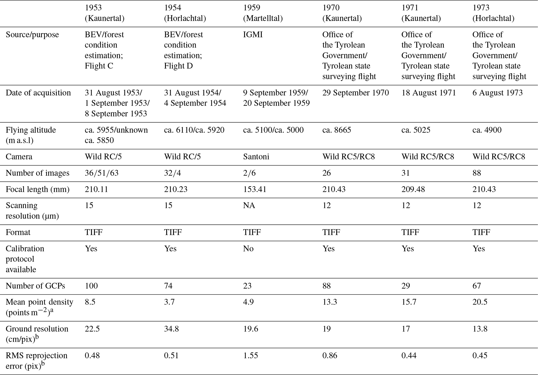
aRefers to the exact sites. bRefers to the entire data set.
3.1.2 Digital elevation model (DEM) and DEM of difference (DoD) processing
Although all point clouds were finally available in the same coordinate system (ETRS89/UTM zone 32N; EPSG code 25832), a local adjustment of each site was carried out to obtain the highest possible accuracy of the subsequent DoDs to be calculated. For this purpose, stable areas, i.e. geomorphologically unchanged areas such as rock outcrops or stable areas on the lateral moraines, were mapped next to each site based on orthophotos. To match the point clouds as well as possible, the iterative closest point (ICP) algorithm (Besl and McKay, 1992; Bakker and Lane, 2017) implemented in SAGA LIS (Conrad et al., 2015) was used for fine registration. Previously, the lidar-based point clouds were further processed in the software SAGA LIS (LIS Pro 3D) from Laserdata (https://www.laserdata.at/, last access: 1 March 2021), in combination with Python and R, to prepare point clouds for the generation of high-resolution digital elevation models (DEMs). This included the removal of outliers (remove isolated points), a ground classification (to remove vegetation), which was carried out with a modified approach according to Hilger (2017), and the achievement of more homogeneous point clouds with the tool 3D Block Thinning (PC) in SAGA LIS. The point clouds were then converted into DEMs using the Point Cloud to Grid tool in SAGA LIS (elevations of points averaged for each raster cell; cell sizes for Horlachtal and Kaunertal are 1 m and for Martelltal 2 m). Finally, the DoDs were generated by subtracting the individual DEMs from each other to determine the positive and negative elevation changes in the Earth's surface.
3.1.3 Data statistics
The presence of various uncertainties in differently generated DEMs (Hodgson and Bresnahan, 2004; Bakker and Lane, 2017) also leads to uncertainties in the resulting DoDs (Lane et al., 2003; Rolstad et al., 2009; Cavalli et al., 2017; Anderson, 2019). Therefore, an uncertainty assessment was carried out using the DoD values from stable areas near each site. The size of the stable areas varied between 25 % and 75 % of the size of the corresponding site. In addition to the estimation of the precision (SD) and accuracy (RMSE), the arithmetic mean, minimum, and maximum values were also determined (Fig. 4).
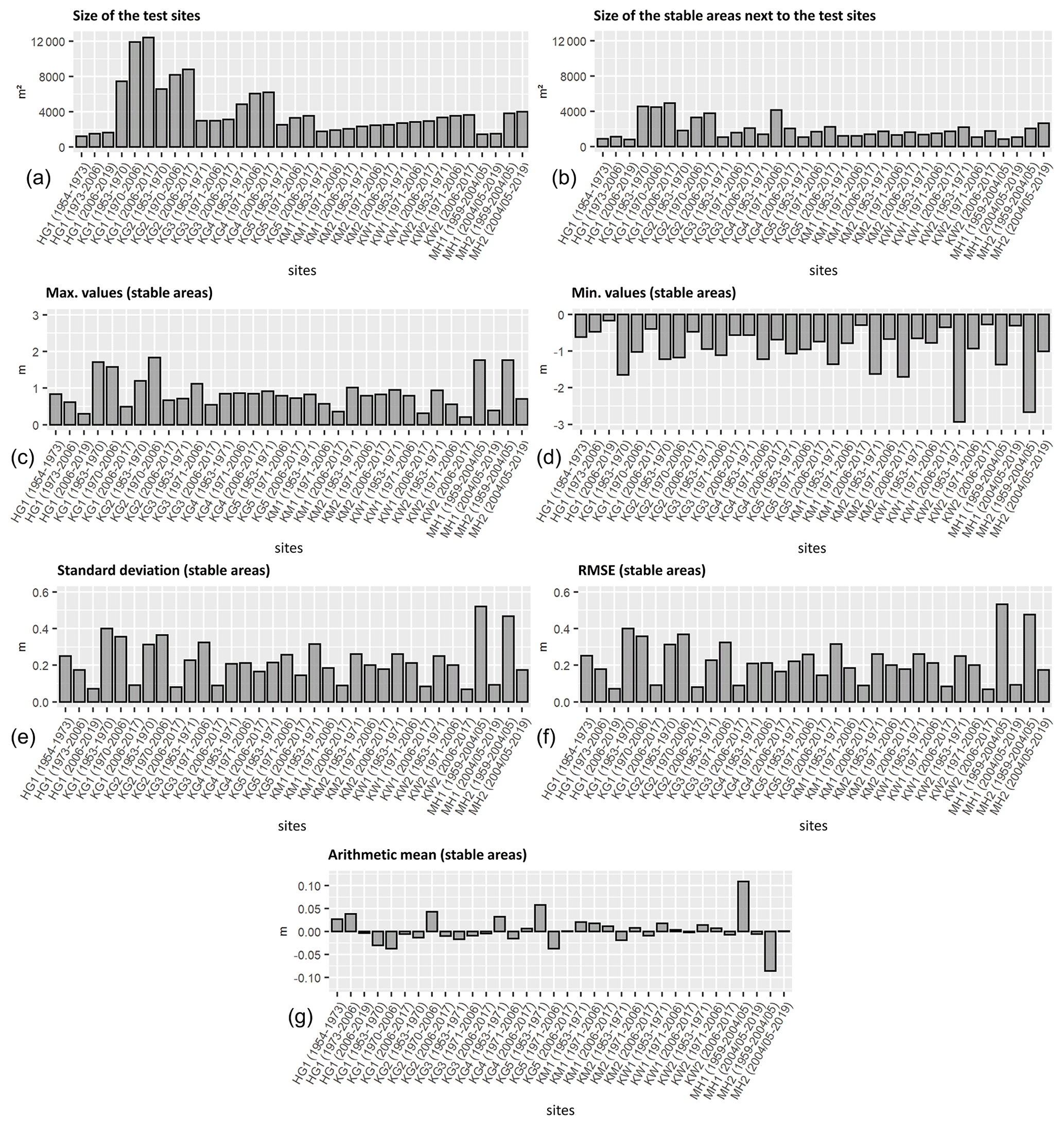
Figure 4Statistical analysis of the uncertainty assessment. (a) Size of the test sites, (b) size of the stable areas next to the test sites, (c) max values (stable areas), (d) min values (stable areas), (e) standard deviation (stable areas), (f) RMSE (stable areas), and (g) arithmetic mean.
To determine the uncertainty in the sediment volume change (total sediment output; Fig. 7), the error propagation method for uncorrelated, correlated, and systematic error according to Anderson (2019) was applied. No threshold has been set for the level of detection of the DoDs, as Anderson (2019) clearly recommends not using this for volumetric calculations as it leads to bias in the results. For the final determination of the total error, the following formula was applied Eq. (1):
where σv, re is the uncorrelated error, σv, sc spatially correlated error, and σv, sys systematic error.
3.2 Derivation of the regression lines
In this study, we followed the sediment-contributing-area approach of Neugirg et al. (2015a, b, 2016) and Dusik et al. (2019), who applied this approach at the slope scale and replaced real sediment traps in the channels, as originally based on the work of Haas (2008) and Haas et al. (2011), using the sediment-contributing-area model, with so-called virtual sediment traps in modelled channels in a DEM (Fig. 5).
The sediment-contributing-area model uses an empirical relationship between the log. sediment-contributing area as the independent variable and the log. mean annual bedload sediment yield as the dependent variable. Thus, the sediment-contributing area can be used as a predictor of sediment delivery in alpine catchments.
Linear regression analysis was used to show this significant correlation, which is formulated as Eq. (2):
where y is the log. mean annual bedload sediment yield, and x is the log. sediment-contributing area.
This has already been confirmed in several studies in both small and large catchments (ranging from hectare to square kilometres) and in different regions such as the Northern Calcareous Alps (Haas, 2008; Haas et al., 2011; Sass et al., 2012; Huber et al., 2015) and the French Northern Alps/Prealps (Altmann et al., 2021). Finally, it can be stated that a linear dependency of two variables x and y on a log–log scale has a fundamentally different behaviour than a usual linear dependency. In our case, we have y=log (sediment yield) and x=log (sediment contributing area). Back-transformation of Eq. (2) using the exp function yields gives the following relation between sediment-contributing area and sediment yield, as seen in Eq. (3):
Thus, the relation between sediment yield and sediment-contributing area is a polynomial of the form . In particular, the slope in the log–log model represents the exponent of the polynomial in the standard model. The relation between sediment yield and sediment-contributing area is (nearly) linear if slope is (close to) one. In this case, the exponential of the intercept in the log–log model represents the slope of the linear relation in the standard model, meaning that independent of the actual size of the sediment-contributing area, 1 m2 provides the same amount of sediment yield, given by exp (intercept). On the other hand, if the slope in the log–log model is considerably greater than one, then the standard model shows polynomial behaviour, meaning that in the same site, increasing the sediment-contributing area provides more sediment yield per square metre. The steps of the sediment-contributing-area approach of this study are composed as follows and were implemented in SAGA LIS and R. The elevation changes in DoDs (using no threshold) generated from multitemporal data were routed downslope and accumulated using the D8 algorithm (O'Callaghan and Mark, 1984). The resulting accumulated DoD values (accDoD) in every raster cell correspond to the net volume of the sediment balance within its contributing area. On steep slopes, accDoD will be negative and represents the sediment yield of this contributing area (Pelletier and Orem, 2014); if it is close to zero, it means that all eroded sediment has been re-deposited within the contributing area. As in the previous sediment-contributing-area studies by Neugirg et al. (2015a, b, 2016), the application of the parameters used in the original sediment-contributing-area model (Haas, 2008; Haas et al., 2011), which lead to the reduction in the hydrological catchment to the sediment-contributing area, is omitted because the sites and the modelled channels are consistently steep, uncovered, and have short slope lengths, making this reduction obsolete. Therefore, the sediment-contributing area is identical to the catchment area in this study.
In detail, channel initiation points were delineated using a threshold of 20 m2 of the flow accumulation that was computed using the D8 algorithm (O'Callaghan and Mark, 1984). Channels that were shorter than 10 m were discarded. To ensure statistical independence through avoiding overlapping contributing areas, a stratified sampling scheme was adopted that included one randomly selected raster cell per channel. Pairs of values (sediment yield and the corresponding sediment-contributing-area size) were randomly extracted from the corresponding channels for each site, and a regression line was calculated accordingly. To quantify the uncertainty due to random selection, this sample was repeated 100 times, resulting in 100 regression models of sediment yield on the sediment-contributing area.
Furthermore, we added two conditions and further developed the sediment-contributing-area approach accordingly. In order to obtain more stable regression lines, the range of values of the sediment-contributing-area size was divided into quartiles (with an equal number of cells within the quartiles) to ensure a homogeneous distribution of the extracted values. Additionally, samples that contained points with a high leverage (greater than 0.5) in the regression model were discarded, and the sampling was repeated until a number of 100 samples was reached.
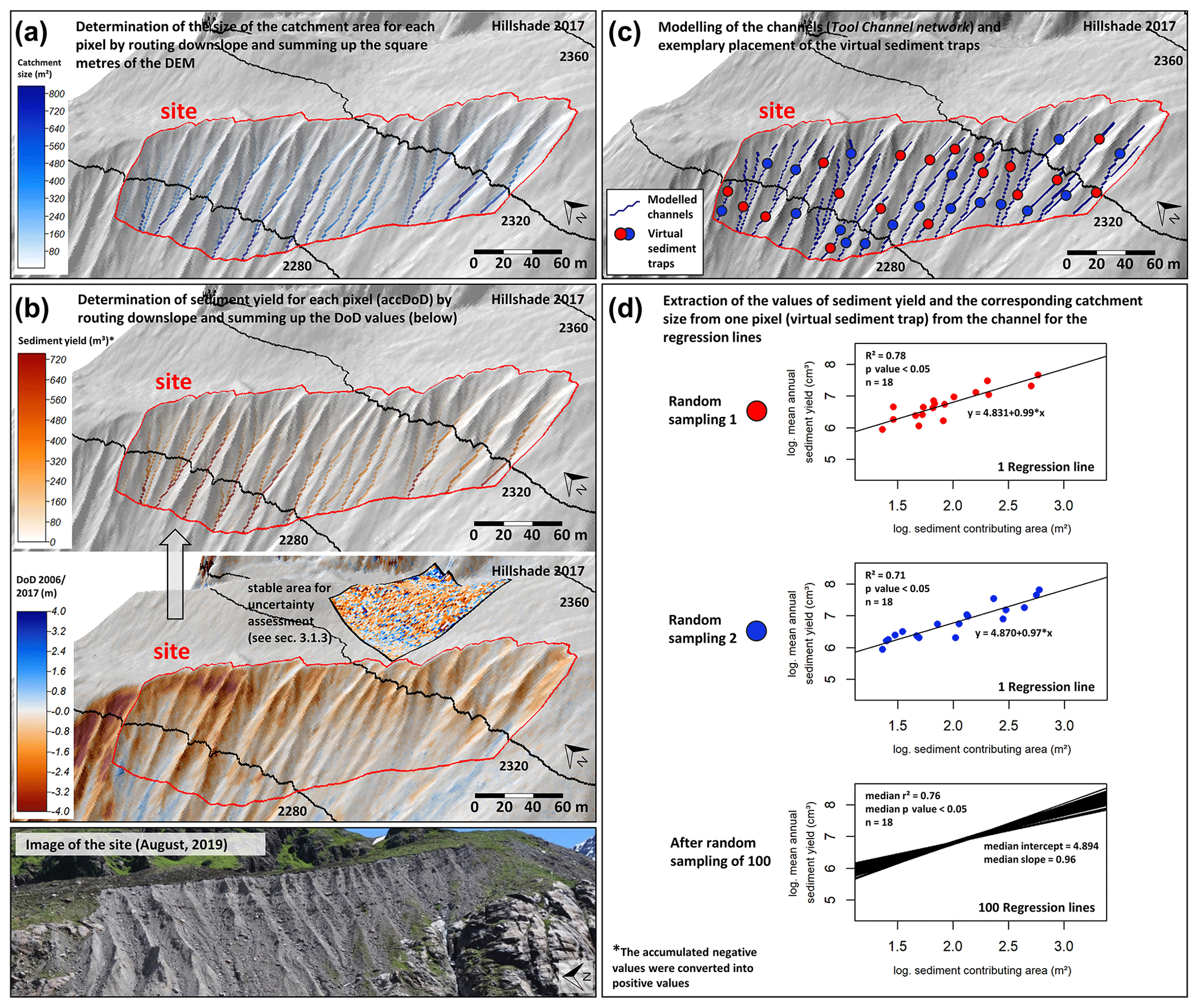
Figure 5Derivation of the sediment-contributing-area approach using the example of test site KG2. (a) Determination of the size of the catchment area, (b) determination of sediment yield, (c) modelling of the channels and exemplary placement of the virtual sediment traps, and (d) calculation of the regression lines.
3.3 Calculation of the sediment output
Additionally, the total sediment output volume, the mean annual sediment output (divided by the corresponding number of years) and the specific mean annual sediment output (additionally divided by the area of the site) were calculated for each site and time period.
The following equation was used for this (Eq. 4):
where Σ DoD is the sum of the corresponding DoD subset values, and L2 is the cell size.
3.4 Generation of meteorological data
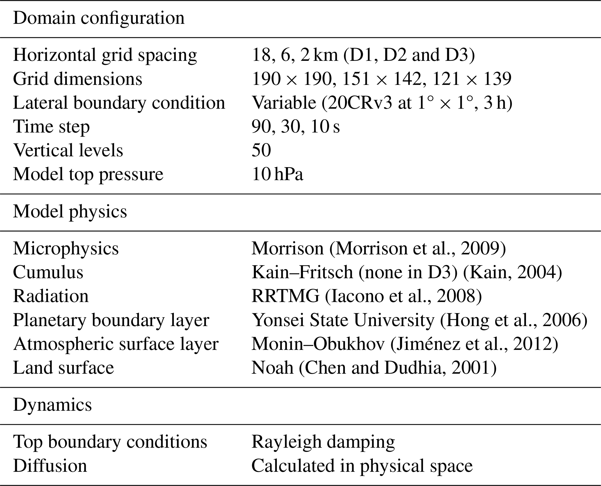
Using data generated with a regional climate model (RCM), the influence of the changes in climate forcing (air temperature and precipitation) on morphodynamics was investigated. For dynamical downscaling of climate data for the beginning of the study period until 2015, we used the Advanced Research WRF (ARW) model of the Weather Research and Forecasting (WRF) model (version 4.3), which is based on fully compressible and non-hydrostatic equations (Skamarock and Klemp, 2008). The Twentieth Century Reanalysis version 3 (20CRv3) data set (Compo et al., 2011; Giese et al., 2016; Slivinski et al., 2019), with a spatial and temporal resolution of 1°×1° and 3 h, respectively, was used as driving data (initial and boundary conditions). The simulation was performed in three nested domains, with grid spacing of 18 (Domain 1), 6 (Domain 2), and 2 km (Domain 3). For our simulations, we mainly used the physics and dynamics options proposed by Collier and Mölg (2020) and listed in Table 5. However, the Noah land surface model, prescribed eta levels by Collier et al. (2019), and the 24 United States Geological Survey (USGS) land use categories were used. The temporal resolution of simulated data in D3 is 1 h for temperature and 15 min for precipitation.
Table 5Overview of the Weather Research and Forecasting (WRF) Model configuration.
The simulated temperature and precipitation data were extracted at the location of each of the five glacier forelands (Fig. 1). These are the centres of the respective sites and represent the corresponding glacier foreland. In addition, a corresponding elevation correction of the climate data was applied for temperature.
For the analysis, we used the mean annual air temperature (2 m above ground), as well as the corresponding trends and the mean number of ice days (days with maximum temperature <0 °C). In addition, the number of warm air inflows from October to May was determined in order to identify corresponding snowmelt processes at the sites. A warm air inflow is defined as a period of at least 3 d in which more than 70 % is above 0 °C, following a previously colder period of 5 d (100 % below 0 °C). In addition, the precipitation patterns were analysed. For this purpose, the mean annual precipitation totals, the mean annual winter (October to May), and the mean annual summer precipitation totals (June to September), as well as the corresponding trends, were determined in order to identify seasonal changes. Furthermore, various continuing classes (4 mm for 1 h resolution and 10 mm classes for daily totals) were used to analyse corresponding changes in individual extreme events and daily precipitation totals. Individual precipitation events were defined as one event, regardless of length, if they were contiguous throughout and were separated if there was no precipitation for at least 1 h. To minimise the noise generated in the data, both data sets were also filtered for extremely small events by changing the values from <0.01 to 0 mm. The calculation of the mean annual winter precipitation was always carried out over the entire winter. For example, for the winter of 1953, data from October 1952 to May 1953 was included. The average summer precipitation was calculated accordingly from June 1953 to September 1953. Furthermore, precipitation was differentiated into snow and rain events. The determination of a threshold to distinguish rain from snowfall is very dynamic in mountainous regions and difficult to estimate. However, the difference between rain to snow depends mainly on surface air temperature, as well as air humidity, with snow occurring mainly between 0 and 3 °C (Froidurot et al., 2014), and the lower the humidity, the higher the probability of snowfall will be. In this study, the threshold from rain to snow was defined at ≤0 °C, as rain is almost excluded below this temperature (Froidurot et al., 2014; Fehlmann et al., 2018).
4.1 Sediment-contributing-area approach
All determined regression lines show a positive correlation between log mean annual sediment yield and log sediment-contributing area (Fig. 6; Appendix A), which means that sediment yield increases with the corresponding sediment-contributing area. In the following, only the median of the 100 regression lines (median slope) of all sites and time periods is used to qualitatively describe corresponding differences. Mostly, there is a decrease in sediment yield between the different time periods and a decrease in the slopes of the regression lines, which is due to a decrease in sediment yield per square metre of the sites. With regard to Sect. 3.3, a decreasing intercept together with an almost constant, although slightly decreasing, slope close to one can be seen over the different time periods in the log–log model, indicating that the relation between sediment-contributing area and sediment yield remains almost constant. The sites KG3, KG4, KM1, KM2, and KW2 show such a behaviour. On the other hand, the areas KG1, KG2, KG5, KW1, and MH2 show clearly larger differences in the time periods. In the earliest time period, the slopes considerably larger than one (in the log–log model) show polynomial behaviour, which means that in the same site an increasing sediment-contributing area provides clearly more sediment yield per square metre. In the later time periods, the slopes also tend towards one, so that the models of the different groups become similar. In addition to this general trend (10 sites), an increase in sediment yield and an increase in the slope of the regression line for site HG1 were observed, showing an increase in sediment dynamics over the time periods in this case, which is in contrast to the previous observations. Site MH1 shows a similar level of sediment yield (between the time periods) with higher slopes of the regression lines, also indicating an increase in sediment yield. Furthermore, slopes of the regression lines below 1 occur in all time periods but especially in the second and third.
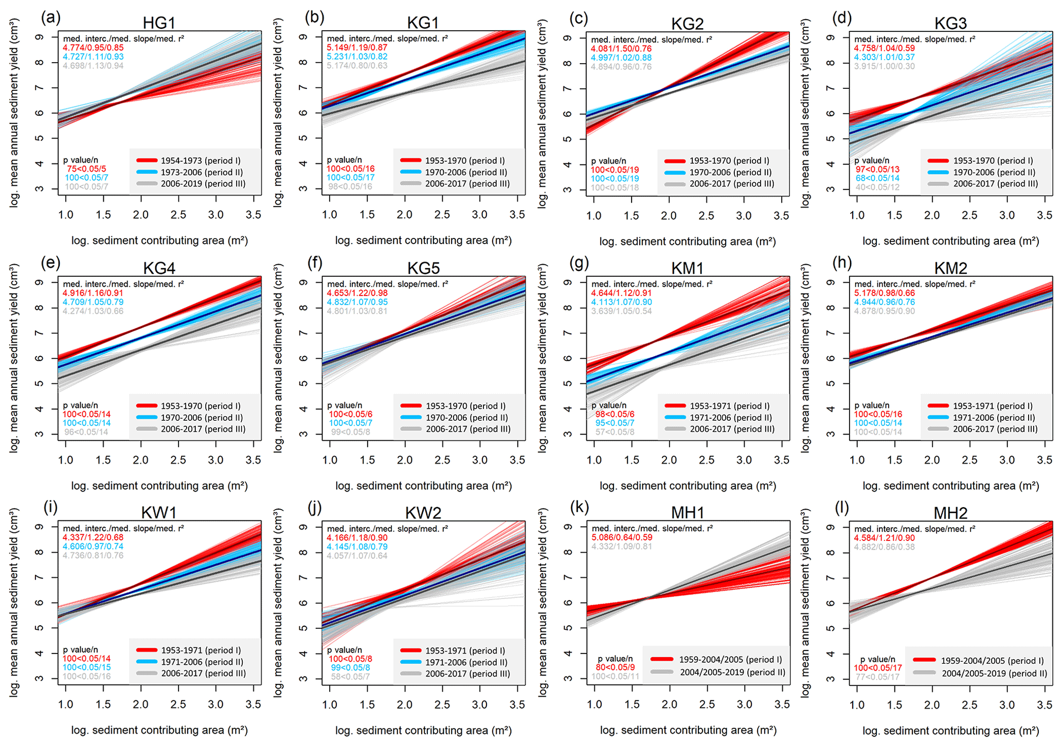
Figure 6Relationships between log sediment-contributing area and log sediment yield for 100 samples of each site and the corresponding time periods. In addition, the median regression line (median slope) is represented by a slightly thicker and darker line.
4.2 Volume calculations of the sediment output
The analyses of the sediment output of the sites confirm the results of the sediment-contributing-area approach (Fig. 7). In general, there is a clear and continuous decrease in mean annual sediment yield of 10 sites over the different time periods. In contrast to this trend, site HG1 shows a clear increase in mean annual sediment yield. Site MH1 also shows an increase but at a very low level, which can also be described as a geomorphic activity of a similar level. In total, the mean annual sediment output decreases across the different time periods. Nevertheless, there is also very high temporal and spatial variability in this change at the sites HG1 and MH1, which also shows a clear increase in geomorphic activity, as well as a slight increase (respectively activity at the same level).
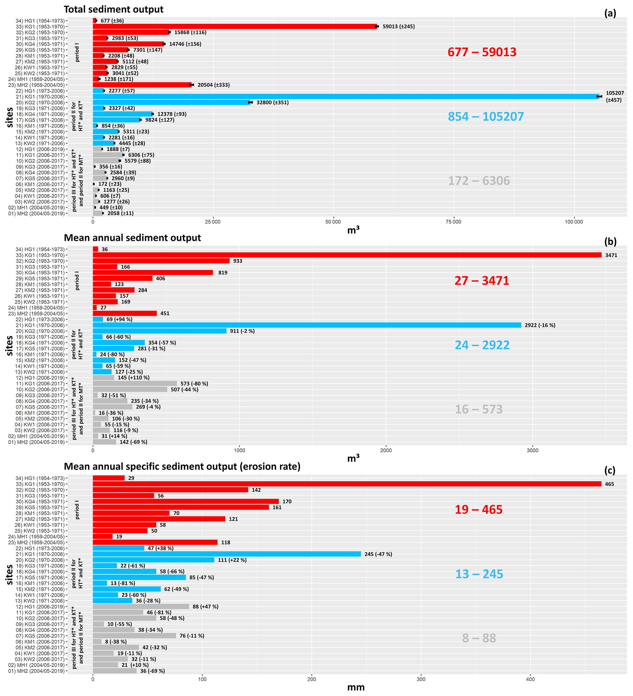
Figure 7Bar plots of total sediment output (with error range according to Anderson, 2019; see Sect. 3.1.3 and 3.4), mean annual sediment output, and mean annual specific sediment output (erosion rate) of each site and time period.
4.3 Meteorological regime
4.3.1 Air temperature
The mean annual air temperature (2 m above ground) of all selected positions of the glacier forelands shows a statistically significant warming trend over the entire study period of 60, 64, and 65 years (Fig. 8). Overall, there is a positive total change of + 1.75 °C (annual trend 0.03; p value <0.05; R2 0.39) for the Horlachtal/Grastalferner glacier forelands; + 1.68 °C (annual trend 0.03; p value <0.05; R2 0.38) for the Kaunertal/Gepatschferner glacier foreland; + 1.70 °C (annual trend 0.03; p value <0.05; R2 0.38) for the Kaunertal/Gepatschferner Münchner Abfahrt (MA) glacier foreland; for the Kaunertal Weißseeferner glacier foreland of + 1.64 °C (annual trend 0.03; p value <0.05; R2 0.36); and for the Martelltal Hohenferner glacier foreland of +2.23 °C (annual trend 0.04; p value <0.05; R2 0.45).
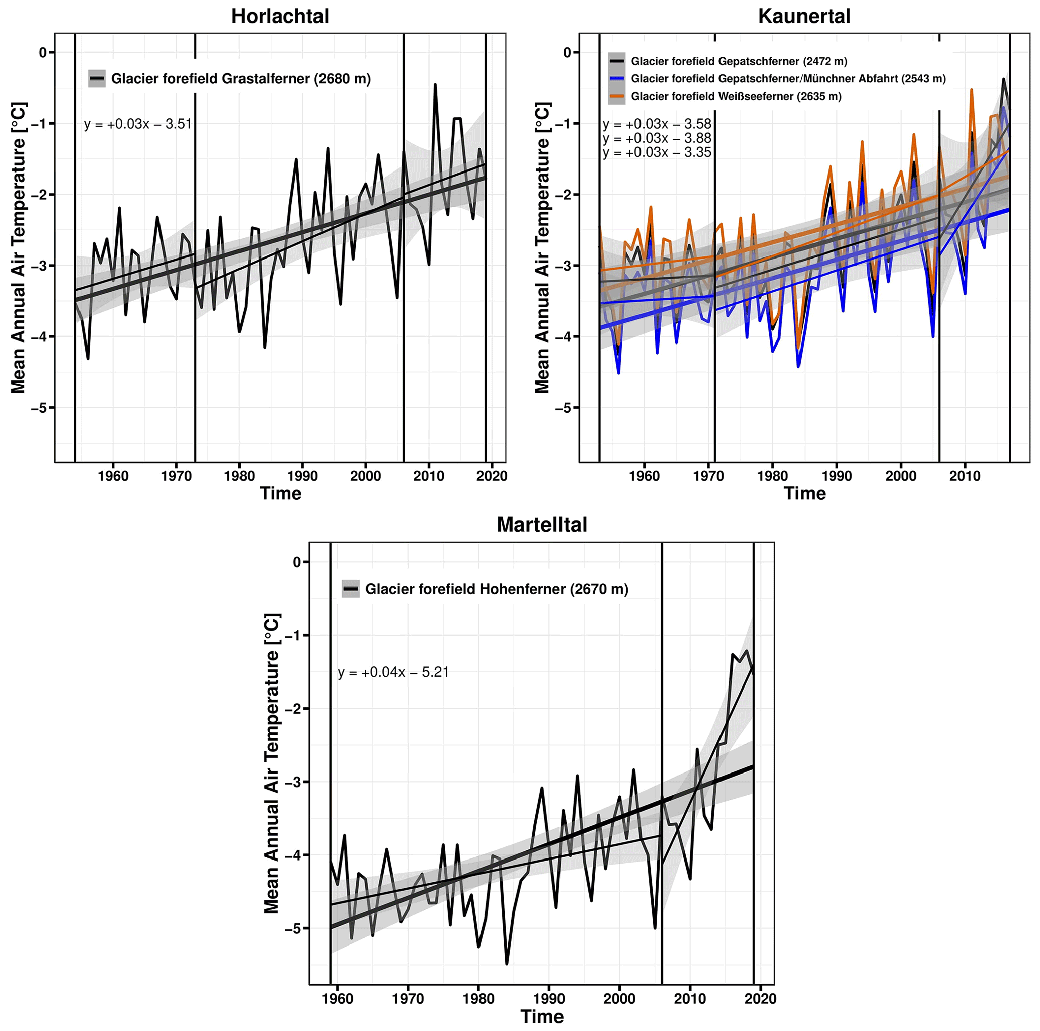
Figure 8Mean annual 2 m air temperature of the glacier forelands within the study periods (95 % confidence interval is included).
The analysis of the mean annual ice days shows a decrease between the time periods, especially from the second to the third time period (in the Martelltal from the first to the second), with a decrease in ice days between 18.4 and 20.7 d, which corresponds to almost 3 weeks (Fig. 9). The analysis of the mean annual warm air inflows shows a decrease from the first to the second time period in the glacier forelands of Grastalferner, Gepatschferner, and Gepatschferner MA and a more pronounced increase from the second to the third time period. In the glacier foreland of Weißseeferner, there is a consistent increase, with the latter being equally more pronounced, whereas in Martelltal there is only a slight increase. Thus, the number of warm air inflows has generally increased.
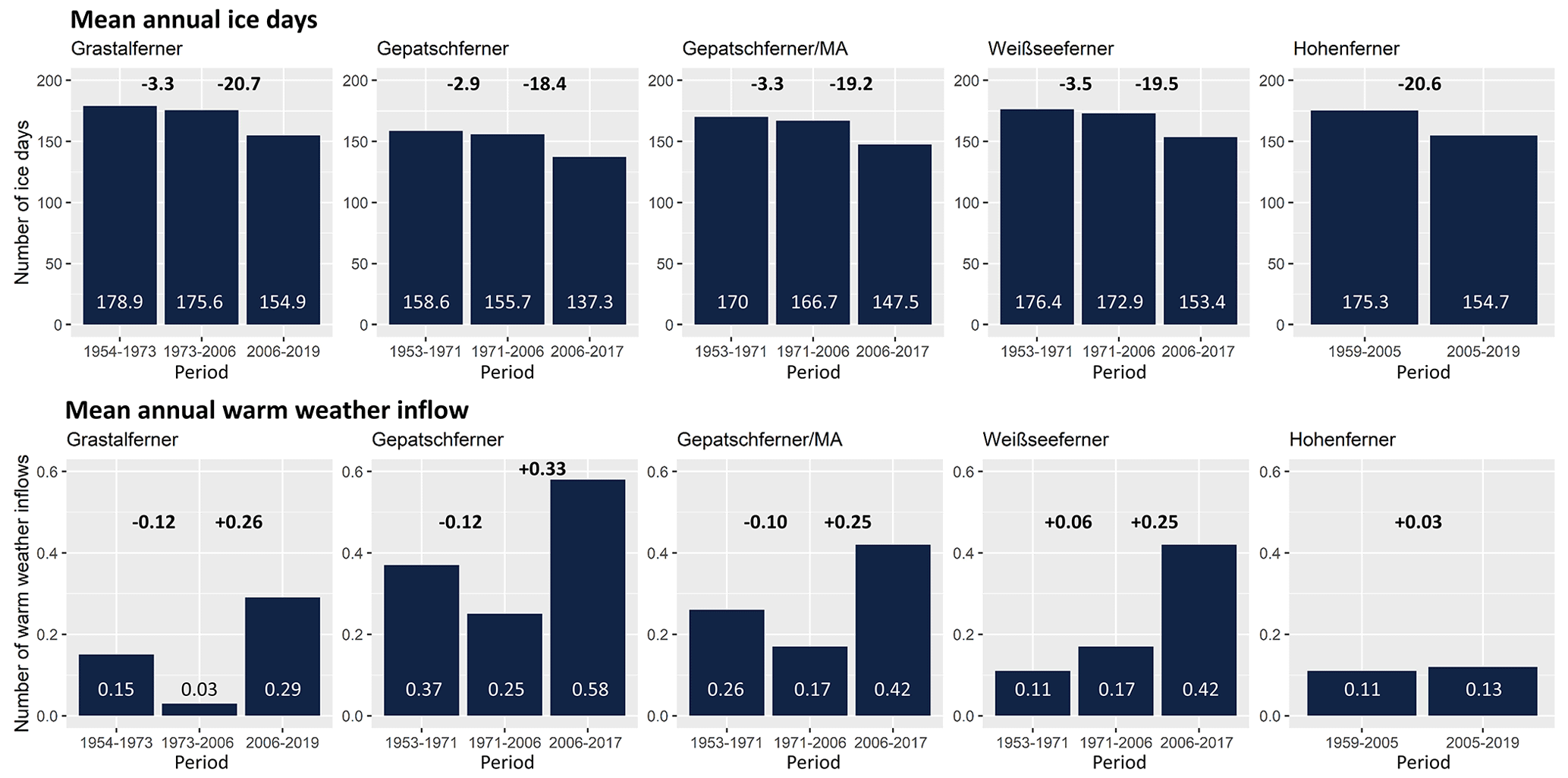
Figure 9Mean annual ice days and mean annual warm weather inflows with the corresponding changes between time periods.
4.3.2 Precipitation
Over the entire time period (60, 64, and 65 years), all study areas show a decreasing trend in mean annual, mean summer, and mean winter precipitation (with the exception of summer precipitation in the Martelltal, which shows a positive trend) (Fig. 10). However, only the changes in winter precipitation (entire study period), summer precipitation (second time period 2004/2005–2019) in the Martelltal (Hohenferner glacier foreland), and annual precipitation (third time period 2006–2019) in the Horlachtal (Grastalferner glacier foreland) are statistically significant, although the latter both cover only 13 and 14 years. In the Horlachtal, the first two time periods show a decreasing trend in precipitation, while the third time period shows an increase in precipitation, which is significantly more pronounced in summer than in winter. In the Kaunertal, winter precipitation shows a slight increase in the first time period and a stronger decrease in summer precipitation. The second time period shows a slight increase in summer and a slight decrease in winter. The third time period also shows a strong decrease in summer and winter precipitation. In the Martelltal, on the other hand, winter precipitation decreases significantly, and summer precipitation increases significantly, especially in the second time period, although time periods of different lengths are analysed.
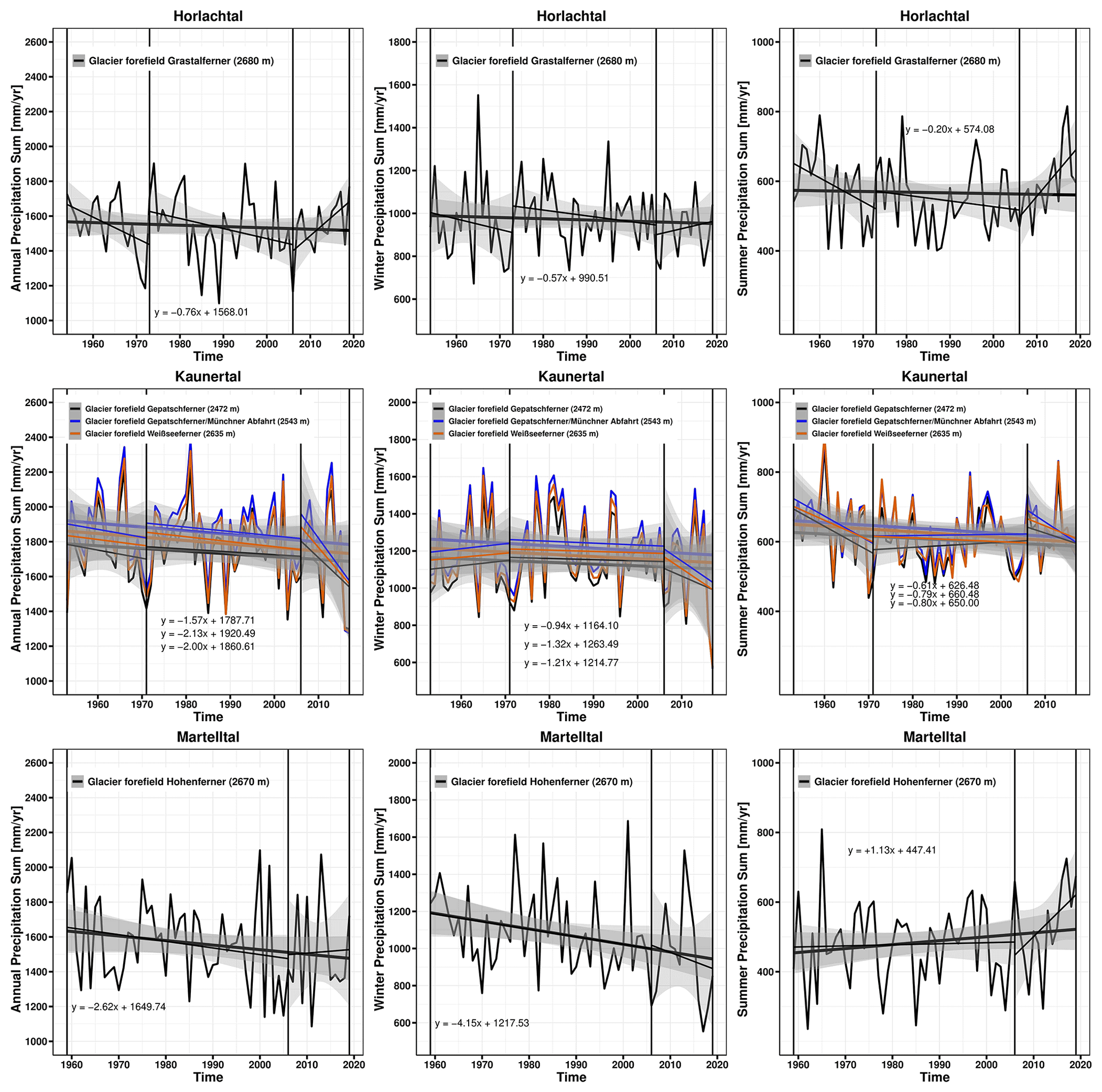
Figure 10Mean annual, mean summer, and mean winter precipitation of the respective glacier forelands.
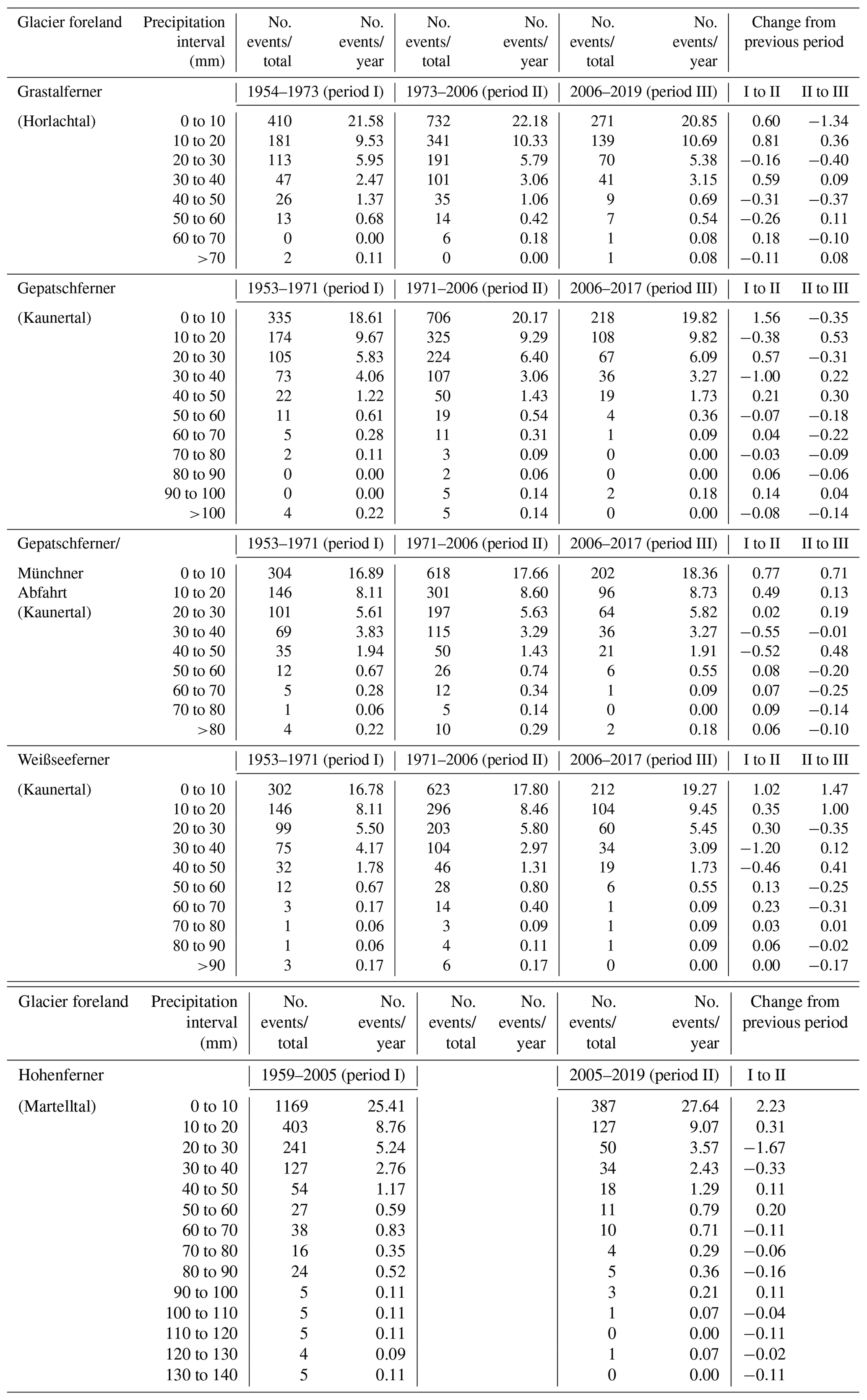
In the following, the changes in different precipitation classes (as well as with a different temporal resolution) between the individual time periods are analysed. The calculated changes are based on Appendix B and C. In these tables, the number of all precipitation events of the corresponding time periods is shown and divided into corresponding precipitation classes. Using the number of years per time period, this results in an mean annual number of events per class. The calculated changes result from the comparison of the mean occurrence of the precipitation classes of the previous time period. Both precipitation events with a resolution of 1 h (Fig. 11 and Appendix B) and daily precipitation totals (Fig. 12 and Appendix C) were analysed. The highest temporal resolution (1 h) shows that the classes >0 to 4 and 4 to 8 are subject to the highest variations (Fig. 11); for example, precipitation events of the class >0 to 4 occur 7.63 fewer times in the glacier foreland of the Grastalferner in the second time period compared to the first. In general, it can be seen that the higher precipitation classes tend to decrease, albeit very slightly, but there are still changes with both an increase and a decrease in the different precipitation classes. The daily precipitation totals also show a high variation, with both a decrease and an increase over the different time periods (Fig. 12). In general, there are also very slight changes. Nevertheless, the decrease in the higher three classes predominates when comparing the third with the second time period.
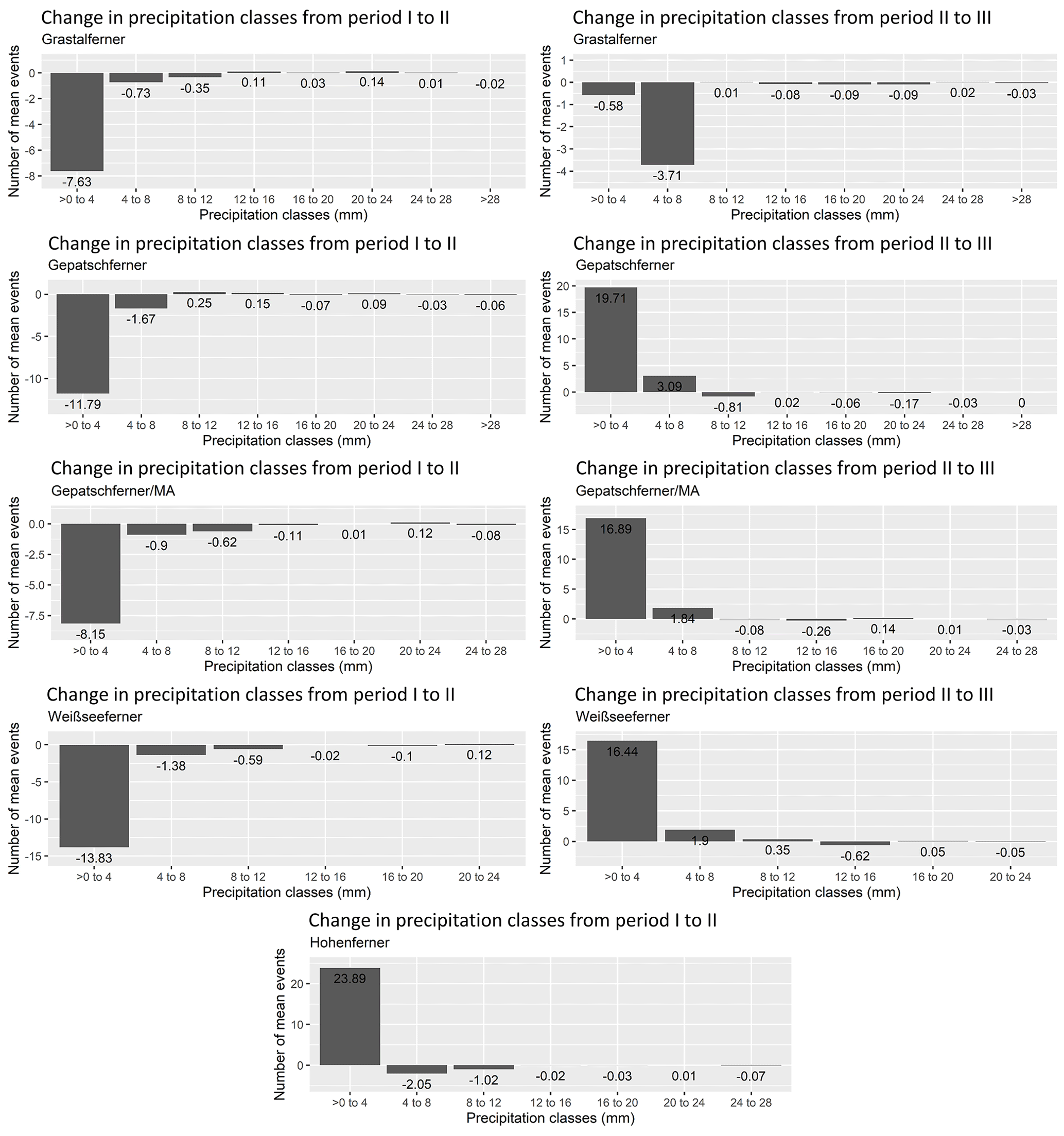
Figure 11Change in precipitation classes between the different time periods with a 1 h resolution (extreme precipitation events).
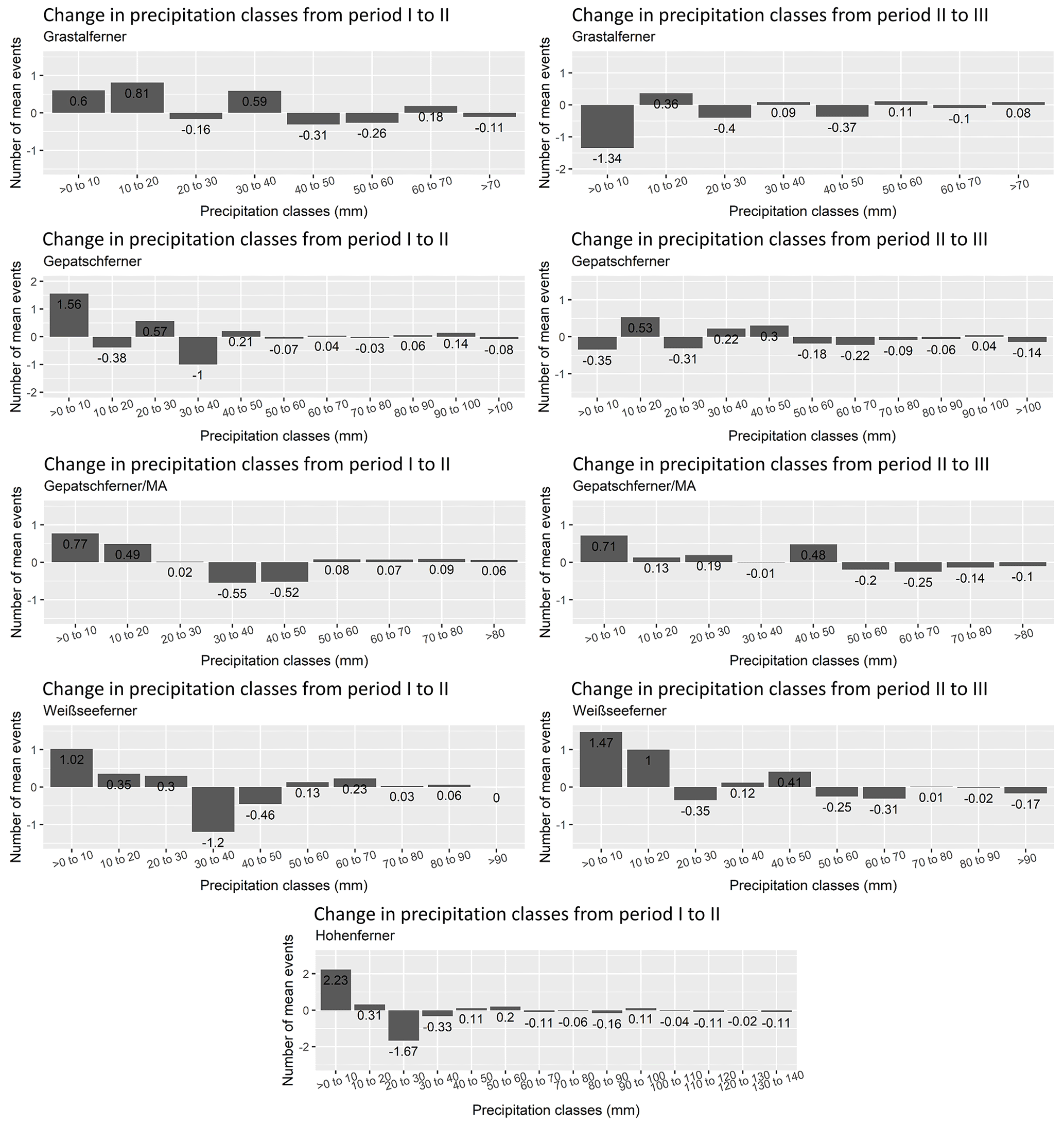
Figure 12Change in precipitation classes between the different time periods with a 24 h resolution (daily precipitation totals).
The analysis of the mean annual rainfall and snowfall events shows that there is a consistent increase in rainfall and at the same time a consistent decrease in snowfall (except for the Weißseeferner glacier foreland) (Fig. 13).
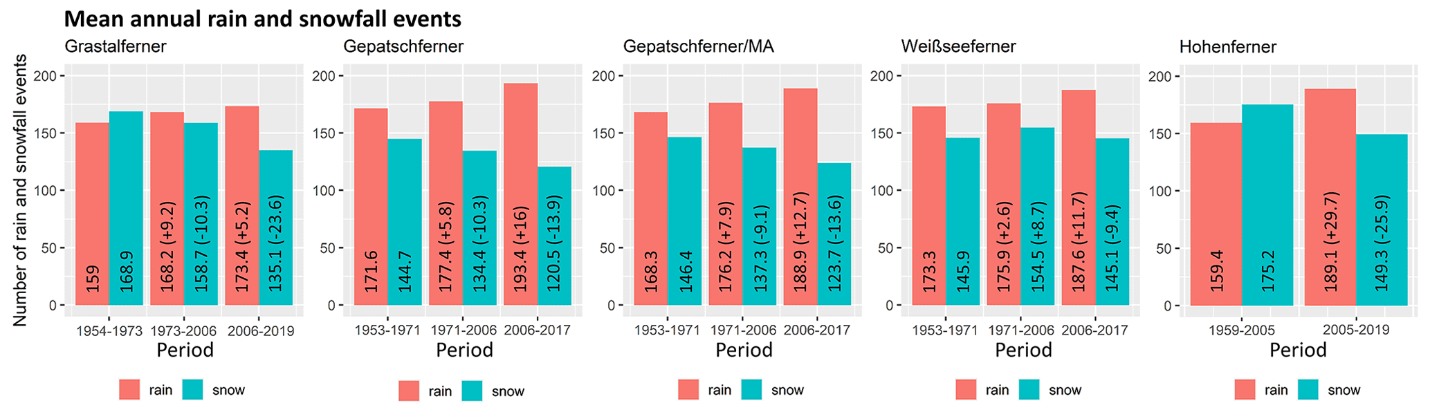
Figure 13Mean annual rain and snowfall events with the corresponding changes between time periods.
5.1 Assessment of the sediment-contributing-area approach
Using the relationship between accumulated sediment yield from DoDs and sediment-contributing area/catchment area (log–log model) of different sites and different time periods, we show a long-term monitoring of several geomorphologically active sections of the LIA lateral moraines. This is a clear difference compared to previous studies that used the space-for-time substitution (SFTS) approach in proglacial areas, in which studies used recent morphometric or morphodynamic differences between sites located along a gradient of deglaciation age to infer long-term changes in morphodynamics (Ballantyne and Benn, 1994; Curry, 1999; Curry et al., 2006). This means that long-term studies with quantitative data are rare (Schiefer and Gilbert, 2007; Betz et al., 2019; Altmann et al., 2020; Betz-Nutz, 2021; Betz-Nutz et al., 2023). The approach shown here provides reliable results and requires only a few input data (Neugirg et al., 2015a, b; 2016; Dusik, 2019; Dusik et al., 2019). The results mainly show a decrease in sediment yield, as well as a decrease in the slope of the regression lines (suggesting less sediment yield per square metre) over the different time periods, indicating a decrease in geomorphic activity at these sites. In some sites, we observe contrasting changes. There is an increase in sediment yield and an increase in the slope of the regression line at HG1 and almost no change in sediment yield on the y axis but an increase in the slope of the regression line at MH1, which can be described as an increase (HG1) and a constant geomorphic activity (MH1). Moreover, in the earlier time periods, a clearly higher variability in the sediment yield (slope of the regression line clearly higher than 1) was observed at the respective sites, which is no longer reached in the later ones. Thus, it is possible to describe two different types of change in sediment yield (size of sediment yield between time periods and variability in the sediment yield within a time period, which can also be compared with the other time periods). Slopes of the regression line below 1 could occur when spots appear within the area that are no longer active, which could be an indication of stabilisation, which occurs mainly in the second and third time period.
The p values of the coefficients are mostly below the alpha level of 0.05, so it is assumed that the relationships between sediment-contributing area and sediment yield are statistically significant in almost all cases (∼92 %) (Fig. 6). To determine the proportion of the variance in the dependent variable that can be explained by the independent variable, the R squares (R2 or the coefficient of determination) of all regression lines were analysed (Fig. 6; Appendix A). The relationship between sediment-contributing area and sediment yield shows varying correlations within the site and the time periods. The median R2 values range from 0.59 to 0.91 in the first time period, from 0.37 to 0.93 in the second time period, and from 0.3 to 0.94 in the third time period (Fig. 6; Appendix A). The number of channels modelled differed between the time periods at the same sites due to the different quality of the DEMs and the slightly different size of these. As in Heckmann and Vericat (2018), the accumulation of DoD values resulted in very small positive values at some sites. Such errors are due to the quality of the DoD, different bulk densities of eroded vs. deposited materials, and the inability of the flow-routing algorithm to fully reproduce sediment transfer in reality especially when flow directions changed within one time period. Where positive accDoD values occurred, they were small and manually corrected to the zero.
Nevertheless, the D8 algorithm simplifies complex sediment transport processes such as fluvial activity, landslides, and debris flows, which have different frequencies, magnitudes, and forms of erosion and accumulation. As the individual time periods cover several years, no reference can be made in this study to individual processes that can be attributed to extreme precipitation events or to seasonal differences. Therefore, we compare different time periods based on mean annual sediment yield, which includes all geomorphological processes. Accordingly, the aim was not to model individual erosion processes but to compute sediment yield of each cell. The individual sites have a slightly different area within the different time periods, which is mainly due to headcut retreat (Heckmann and Vericat, 2018; Betz-Nutz et al., 2023). The lateral boundaries also changed slightly due to the quality of the DEMs and geomorphological slope processes, while the lower boundary did not change.
By processing historical aerial photographs into DEMs (by SfM–MVS), the temporal aspect of sediment-contributing-area studies could be quickly and cost-effectively extended to several decades (up to the 1950s), which previously spanned only a few months or several years (Neugirg et al., 2015a, b, 2016; Dusik, 2019; Dusik et al., 2019). However, as Schiefer and Gilbert (2007) have already shown, the shorter the time intervals and the lower the quality of the aerial images, the more difficult it becomes to detect surface changes, so in the process of this study, several series of aerial images had to be sorted out that were actually available due to a poor data quality. Furthermore, it should be noted that the accuracy and precision of the historical DEMs strongly depend on the respective generation, for example, whether they were generated with or without a calibration certificate (as was the case, for example, with the 1959 aerial photo series in the Horlachtal/glacier foreland Hohenferner), which ultimately influences the sediment-contributing-area results and the calculated erosion rates (Stark et al., 2022).
5.2 Geomorphic activity
The geomorphic activity is directly related to the characteristics of the sites. The sites with the highest mean annual sediment output (> 100 m3 yr−1) (such as KG1, KG2, KG4, KG5, MH2, KM2, and KW2) show strong gully formation and are overall characterised by larger areas, longer max slope lengths, and higher mean and max slope gradients (Table 1). In contrast, the sites with lower mean annual sediment output (<100 m3 yr−1) (such as KW1, KG3, HG1, KM1, and MH1) show less gully incision. These sites tend to be characterised by smaller areas, smaller max slope lengths, and smaller mean slope and max slope gradients (Table 1). The strong influence of slope length and slope gradient on morphodynamics is also shown by previous studies (Ballantyne and Benn, 1994; Curry, 1999; Curry et al., 2006; Betz-Nutz et al., 2023). KG3 also appears to be somehow stabilised by bedrock in the lower part of the slope, which could mitigate the erosion of this site, as also shown by Jäger and Winkler (2012). Elevation and aspect, however, do not seem to have an influence on geomorphic activity, which is also shown in the study by Curry et al. (2006). Since only bare and sparsely vegetated areas were investigated, no findings on the influence of vegetation on morphodynamics can be made in this study. Solifluction processes could also not be observed, probably due to the composition of the moraine material. Presumably, the morphodynamics are still so high that the vegetation does not yet have the opportunity to develop accordingly. In general, we assume that debris flows are the most common process, as described, for example, by Ballantyne (2002a) and Curry et al. (2006). Thus, material stored in the gullies is transported downslope by debris flows mainly as rain or snow events in the spring or heavy rainfall events during rainstorms in the summer months (Ballantyne and Benn, 1994; Ballantyne, 2002b; Curry et al., 2006; Dusik et al., 2019).
However, the high mean annual sediment yield and corresponding erosion rate in the first (3471 m3 yr−1, 465 mm yr−1) and second (2922 m3 yr−1, 245 mm yr−1) time periods of site KG1 (Fig. 7) can probably also be attributed to individual landslides and deep-seated slope failures that are in some cases linked with melting dead ice bodies, as these processes are more likely to occur after deglaciation and are characterised by high magnitude and low frequency, which has also been shown by Blair (1994), Hugenholtz et al. (2008), and Cody et al. (2020). On the less incised slopes (e.g. MH1), small-scale processes such as fluvial erosion or snow drifts probably occur (Betz-Nutz, 2021), which ultimately show no clear trend in the increase or decrease in the morphodynamics but can be described as a constant geomorphic activity. In Betz-Nutz et al. (2023) and in this study, six similar lateral moraine sections (although other exactly defined sites) were investigated. The test sites KG1, KG2, KW1, KW2, and MH1 (in Betz-Nutz et al., 2023; GPF1, GPF2, WSF1, WSF2, and HF1) showed similar erosion rates and the same long-term trends. In the case of site MH2, different trends were determined (stagnation in Betz-Nutz et al., 2023, and a decrease in this study), which can be attributed to the differently defined site and the slightly different study period.
In the sense of a process–response system, it is noticeable that the first-mentioned group of sites with the higher erosion rates (except KG1) had considerable influence from melting dead ice in the lower slope area at least until 2006 (KG2, KM2, KW2, and MH2), or the glacier was still present at the bottom of the slope (KG4 and KG5), which could be identified by the interpretation of the DoDs. Melting of the dead ice can lead to destabilisation of the slope, which can enhance erosion processes of the upper slope areas, as the support is no longer present, the sediment becomes saturated, and there can be an increase in the slope gradient due to the subsidence of the lower part of the slope (Altmann et al., 2020; Betz-Nutz et al., 2023). However, the highest slope gradients are also present here, which also plays a major role. In addition, site HG1, where erosion is increasing, shows an undercutting of the slope by the adjacent stream, which leads to a destabilisation or lowering of the erosion base and a typical formation of a debris cone and alluvial fan, with a successive reduction in the slope gradient that is missing (Fig. 14). It can be assumed that individual strong rainfall events in the second and third time periods in combination with changing flow pathes due to the retreat of the Grastalferner acted here as an impulse and affected both the site itself and the adjacent stream.
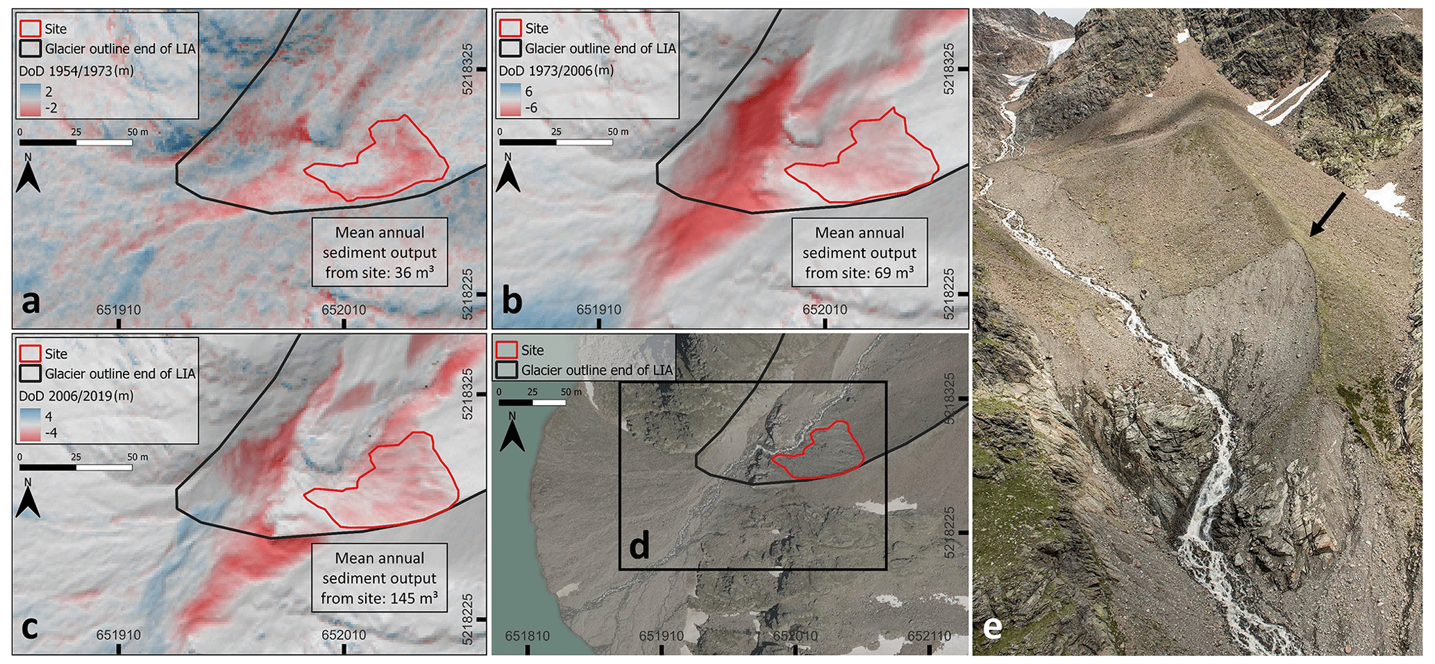
Figure 14Overview of the DoDs of the corresponding time periods of site HG1. (a) DoD 1954–1973, (b) DoD 1973–2006, (c) DoD 2006–2019, (d) orthophoto 2020 (provided by the province of Tyrol), and (e) photo of the site from 2019 by Anton Brandl.
5.3 Paraglacial landscape adjustment
5.3.1 The sediment activity concept
The finding of mainly decreasing geomorphic activity of the LIA lateral moraines in this study is largely consistent with previous model-based studies describing the paraglacial landscape adjustment with a decrease in geomorphic activity in proglacial areas over time, such as the theoretical model “paraglacial concept” of Church and Ryder (1972) or the “sediment exhaustion model” of Ballantyne (2002a, b). The geomorphic activity of gully systems is given as a few decades to centuries (Ballantyne, 2002a, b). Furthermore, it is stated that there is a high temporal and spatial variability in this development. The model provides an appropriate approximation (Ballantyne, 2002a, b). Within the paraglacial adjustment process, different geomorphological processes result in different durations of occurrence. Furthermore, different land systems react at different rates and on different spatial scales. Thus, external perturbations can occur, leading to secondary peaks and time delays (Ballantyne, 2002a, b). While 10 out of 12 sites fit the model descriptions, two test plots show opposite morphodynamics, which can be described as a delay of the paraglacial adjustment process or that the response systems can run counter to such an adaption.
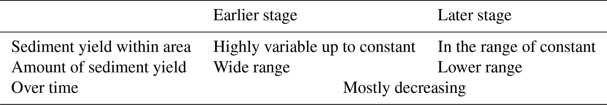
To estimate the changing morphodynamics, we therefore propose the following simplified description of the landscape evolution using the sediment activity concept, based on the results of this study. Due to the study design, this concept is only valid for geomorphologically active areas (in this case, the upper lateral moraine section) on the LIA lateral moraines and until about 170 years after the end of the LIA (Table 6; Fig. 15). The concept distinguishes between an earlier and a later phase. The earlier phase (mainly 1950s to 1970s) is characterised by a wide range between areas with high and low variability in sediment yield within the area, as well as high and low mean annual sediment yield (erosion rate/volume). In contrast, the later stage (mainly 1970s to 2000s and 2000s to the end of the survey 2017/2019) shows a decrease in this range. Although the decrease in the morphodynamics predominates, there are also increases in morphodynamics. The time of ice release was not integrated here, so that the time periods refer to the actual time. In addition, we give two examples in Fig. 15. While example A shows high variability (polynomial behaviour) within the area and high sediment yield (erosion rates/sediment output), example B shows low variability (constant/linear behaviour) and low sediment yield (erosion rates/sediment output). Ultimately, the relationship between sediment yield and the size of the catchment has changed so that erosion within the area is more constant today.
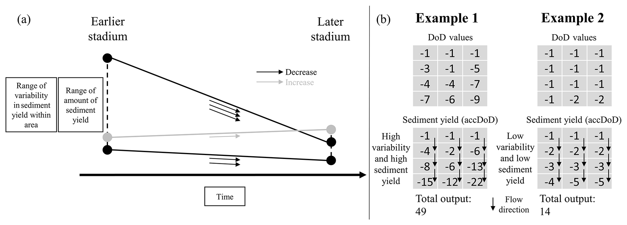
Figure 15The sediment activity concept. Description and illustration of the change in sediment activity over time (a) and two corresponding examples (b).
Through introducing the sediment activity concept of this study, we present a different description of the paraglacial adjustment process which is based on the actual sediment yield. However, the concept is only valid until about 170 years after the end of the LIA and at the sites of this study. The sediment activity concept presented here is also compatible with the results of other studies; for example, Betz-Nutz et al. (2023) mostly show a decrease in erosion rates over a similar time period but also a remaining at similar levels and an increase. In addition, the studies by Church and Ryder (1972), Ballantyne and Benn (1996), Curry (1999), Ballantyne (2002a), Curry et al. (2006), and Schiefer and Gilbert (2007) show a decrease in geomorphic activity over time, which is also consistent with the model presented here. Also, we assume that the concept can also prove its validity in further proglacial active areas and partly over an even longer period of time.
5.3.2 Erosion rates
The methodologies for determining long-term average erosion rates in proglacial areas are based on gully volume estimates (Ballantyne and Benn, 1994; Curry, 1999; Curry et al., 2006) and sediment volume calculations due to surface changes using DoDs, as shown by Betz-Nutz et al. (2023) and this study (Table 7). In glacier forelands in western Norway, this amounts, for example, to minimum estimates of 50–100 mm yr−1 (max estimates of min 200 mm yr−1) (Ballantyne and Benn, 1994) and a minimum of 5.5–169 mm yr−1 (in different glacier forelands) (Curry, 1999). A further study in the Swiss Alps shows erosion rates of min 49–151 mm yr−1 (in different glacier forelands) (Curry et al., 2006). The work of Betz-Nutz et al. (2023) and this study show erosion rates over several decades and distinguish between different time periods, making it possible to show differences between them. Both studies show that the mean erosion rates in the individual time periods decrease (Table 7), although in individual cases there is also a constant and an increase in erosion rates over time. Although there has been a clear decrease in geomorphic activity, stabilisation of the sites is not yet apparent, which means that the paraglacial adjustment is still ongoing. Within this study, we observed that the sites still show a high geomorphic activity even after they have been deglaciated for 76–159 years. A stabilisation of the gully systems, as shown by Curry (2006), cannot be observed. Other studies such as Lane et al. (2017), Dusik (2019), Altmann et al. (2020), and Betz-Nutz et al. (2023) also show the still ongoing paraglacial adjustment processes. Comparing the long-term erosion rates of gully systems from the different studies ultimately shows high variability in the adjustment, as these studies were also conducted using different methods, on different timescales, and in different regions. Differences are probably mainly due to the different local conditions, such as the geomorphological settings; these include, for example, the different characteristics of the lateral moraine sections, such as slope gradient, slope length, time of ice exposure, dead ice influence, and the development of vegetation. Furthermore, the lateral moraines have different sedimentological characteristics related to their genetic origin. In addition, different meteorological conditions prevail in the different regions.
Table 7Studies on long-term erosion rates (several decades) of gully systems on the LIA lateral moraines in different glacier forelands.
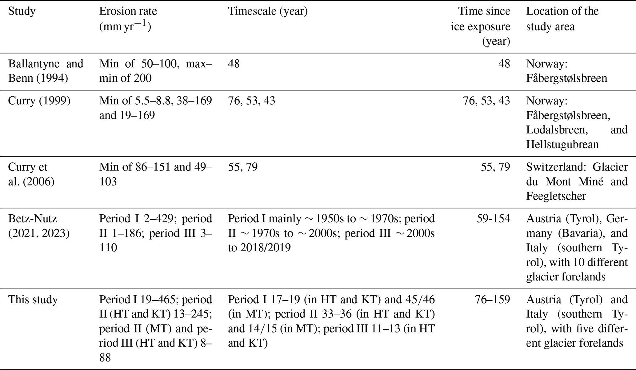
Note: HT is for Horlachtal, KT is for Kaunertal, and MT is for Martelltal.
5.4 Meteorological drivers
The decrease in the mean annual number of ice days and the increase in the number of warm spells over the different time periods and the associated potential increase in snowmelt on the slopes could also lead to an increase in morphodynamics, as these processes represent important preparatory steps for erosion processes in spring (Haas, 2008), such as increased saturation of the slope du to snowmelt, loosening of the upper sediment layers or the delivery of material by snow slides or small wet avalanches that is then available for debris flows in the summer months (Dusik et al., 2019). Klein et al. (2016), for example, also show an increase in the frequency and intensity of snowmelt in the Swiss Alps. Mean annual precipitation decreases slightly across time periods but is not statistically significant (except for winter precipitation for the entire study period (1959 to 2019) and summer precipitation in the second time period from 2005 to 2019 in the Martelltal). Other studies also show that the decrease in precipitation in the European Alps is low (Brugnara et al., 2012), that there is no clear trend in precipitation (Hock et al., 2019), or that it is mainly subject to regional influences and decadal variations (Mankin and Diffenbaugh, 2015). Extreme precipitation events (1 h resolution) and daily precipitation totals also show only minor changes. Differentiation of precipitation, on the other hand, shows a clear increase in rainfall and a decrease in snowfall, which is also shown by Serquet et al. (2011), Beniston et al. (2018), and Hock et al. (2019), who found that the rainfall on snow events in spring as a preparatory factor for the erosion processes in the summer months increase. The simulated meteorological data generally show lower temperatures and larger precipitation amounts when compared to three automatic weather stations operated by TIWAG (Tyrolean Hydropower AG, Innsbruck, Austria). These stations are located in the vicinity of our sites. The simulated mean annual temperatures extracted at the location of the weather stations at Horlachalm (1987–2015) (approx. 6.5 km linear distance to the site in the Grastalferner glacier forefield) and Weißseeferner (2007–2015) (approx. 500 m linear distance to the sites in the Weißseeferner glacier forefield), covering the same time period indicate a difference of −1.05 and of −0.87 °C, respectively, after accounting for differences in elevation. However, at Gepatschalm (2010–2015) weather station (approx. 2.5 km linear distance to the sites in the Gepatschferner glacier forefield), the difference between the simulated and observed mean annual temperatures is 0.13 °C, indicating that the magnitude of the discrepancies depends on the station data used for the comparison. The simulated precipitation, however, is generally larger with mean annual precipitation sums of 1531, 1655, and 1820 mm at the location of Horlachalm (1990–2015), Gepatschalm (2010–2015), and Weißseeferner (2007–2015), respectively, while the weather stations recorded values of 803, 1086, and 924 mm, indicating large discrepancies, especially when compared to Horlachalm and Weißseeferner weather stations. The data sets from which the temperature and precipitation were extracted are both based on coarsely resolved data, which makes a comparison with measurement data in the field difficult, although the corresponding trends are able to be used well for this study. The large difference between simulated and recorded precipitation is mainly due to winter precipitation (Fig. 11) when the weather stations are not always able to record total snowfall accurately; additionally, fog precipitation or precipitation in combination with stronger winds are not recorded correctly.
The weather and climate study periods are based on the predefined study time periods given by the availability and quality of orthophotos and not on the usual climate periods. This results in large differences in the length of the different time periods, which must be taken into account.
There are several sources of uncertainty in the simulated data, amongst them the dynamic initial and boundary conditions, as the forcing data have their own sources of uncertainties. Furthermore, the choice of the reanalysis data used for forcing the model has an influence on the final results. Additionally, for such a long simulations, an updated sea surface temperature (SST) is recommended. Since there are no SSTs available for the 20CRv3, we have generated SST fields from the skin temperature. Other sources of uncertainty are the static boundary conditions like the fixed land use categories and topography, as well as model simplifications and choices in the parameterisation of the physics and dynamics. In our simulations, we have used spectral nudging in order to keep the model from large deviations from the forcing data. Short test runs indicate that the use of spectral nudging improves the simulated data, especially with respect to precipitation. However, the strength of nudging also has an influence on the final results. Since the purpose of this study is not to test how strongly to nudge, we have used the default values in WRF.
Using DoDs based on SfM photogrammetric and lidar data DEMs, we show, with two different approaches, the long-term (1953–2019) change in the morphodynamics of several active gully systems on the LIA lateral moraines in the Tyrolean and southern Tyrolean Alps, Austria, and Italy. First, we show the change in the range of variability in the sediment yield within the area (using regression lines with accumulated sediment yield and sediment-contributing area/catchment area), and second, we show the change in the amount of sediment yield (calculation of erosion rates/volume of sediment output) between the different time periods could be shown.
Finally, the first time period shows a clearly higher range of variability in the sediment yield within the site than the later time periods. This means that the spatial pattern of erosion has become more uniform within the areas. In addition, the total sediment yield, the mean annual sediment yield, and the mean annual specific sediment yield (erosion rate) were calculated for each site, and the time period was calculated. Over the time periods, there is a decreasing trend of geomorphological activity in 10 out of 12 sites, while 2 sites show an opposite trend, where morphodynamics increase or remain at the same level. Overall, we confirm the general trend of decreasing morphodynamics over time (10 sites) of several previous studies, although we could also show that the geomorphic activity of one site is on the same level and one is increasing. Finally, the results led to the proposal of a simplified conceptual model called the sediment activity concept, which describes the paraglacial adjustment process by summarising the findings on the long-term morphodynamics of the upper parts (gully heads) of lateral moraines from this study.
Despite the general decline in morphodynamics, the sites show no stabilisation, leading us to the conclusion that the paraglacial landscape adjustment is still in progress (even on areas that have been ice-free for at least 159 years). It seems that the vegetation has not yet had the opportunity to develop due to the high morphodynamics. In general, debris flows are probably the most common processes, although it is difficult to separate the different processes but very high sediment yield (mainly in the first time period) also indicate landslides and slope failures. Site morphodynamics are also related to the characteristics; i.e. sites that are larger, have longer max lengths, and higher mean slope gradients (as well as max slope gradients) have clearly higher geomorphic activity and form more deeply incised gullies. In the sense of a process–response system, it can be stated that the melting of dead ice in the lower-slope area, which in some cases lasts for decades, leads to high morphodynamics of the upper-slope area. Furthermore, it is assumed that the lowering of the erosion base by adjacent streams leads to a delay of the paraglacial landscape adjustment, as the formation of an accumulation area is disrupted.
In addition to the system internal influences on morphodynamics, we assume an additional influence of changing weather and climate factors on the corresponding erosion processes with an increase (mainly in the last, i.e. most recent, time period from the mid-2000s to 2017/2019), since the statistically significant warming of the last few decades has led to a reduction in the number of mean annual ice days, to an increase in warm air inflows, and, when distinguishing between rainfall and snowfall, to an increase in rainfall. We do not see any clear influence in the changing precipitation, although it can be assumed that the same precipitation intensities led to higher erosion in the first time period than in the second or third. Nevertheless, the system internal dynamics and the general paraglacial adaptation process seem to have the greatest impact on the changing morphodynamics. Future work should apply the approach used here to more areas and, if possible, with a higher temporal resolution to improve the process understanding of erosion on lateral moraines.
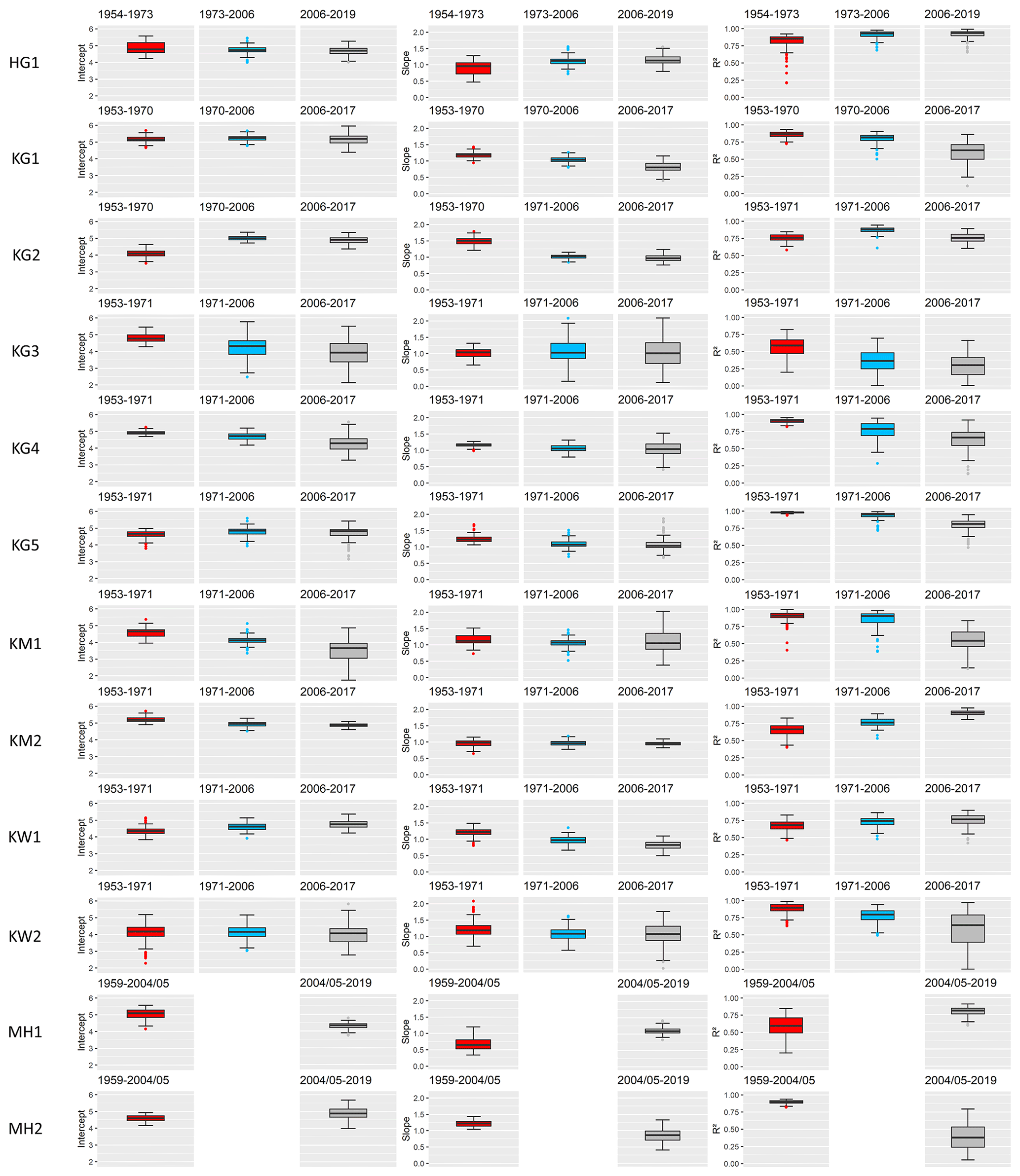
Figure A1Box plots of the model parameters intercept, slope, and R2 of all regression lines (see Fig. 6).
Table B1Calculation of the individual extreme events by continuous ongoing 4 mm classes (with 1 h resolution).
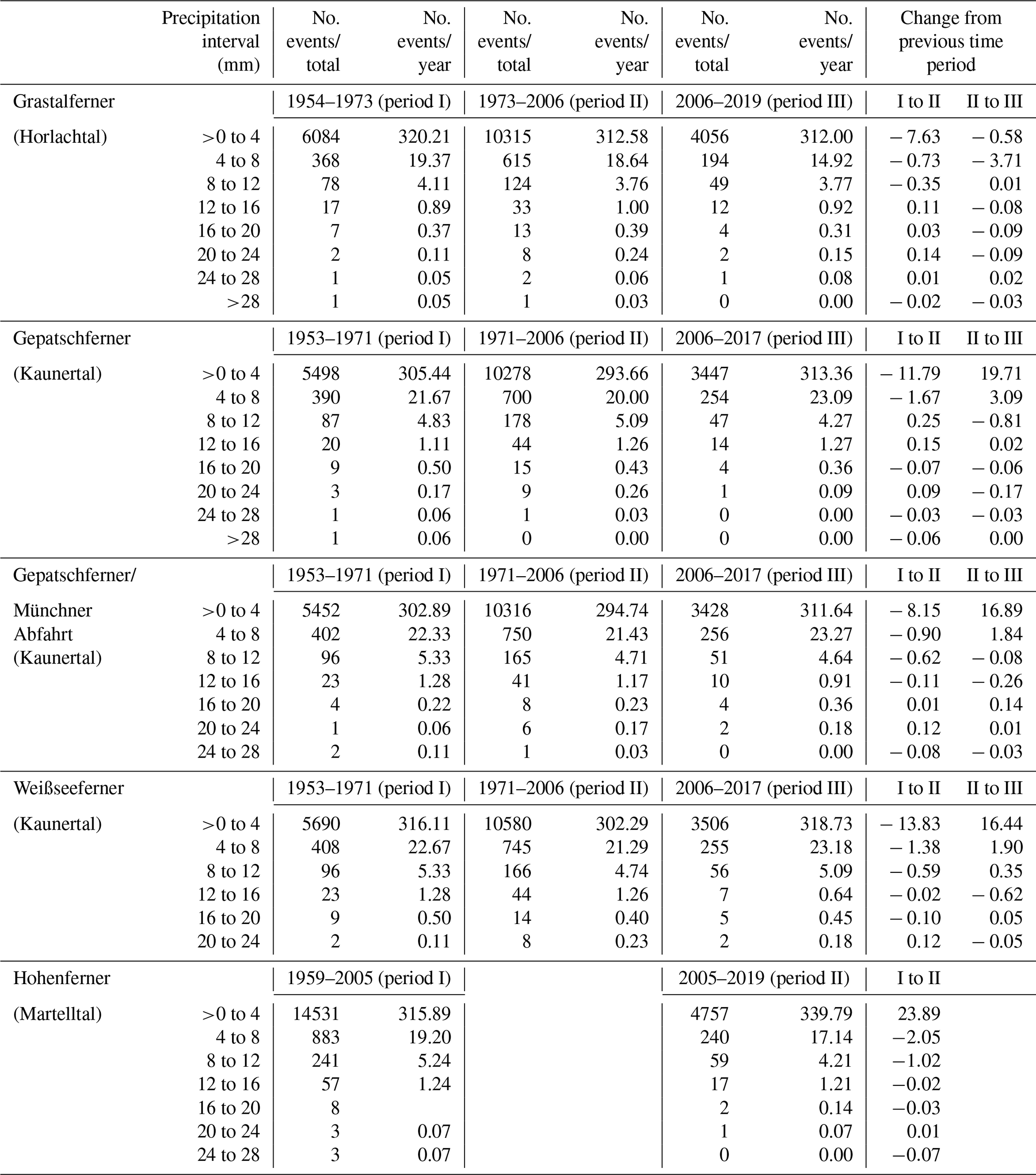
Table C1Calculation of the daily precipitation totals by continuous ongoing 4 mm classes of the different time periods (24 h resolution).
The processing of the historical aerial images into point clouds (and orthophotos) was done with the commercial software Agisoft Metashape Professional (Version 1.6.6) (https://www.agisoft.com/, Agisoft LLC, 2021). These point clouds and the point clouds based on lidar data (ALS) were further processed in the commercial geoinformation system SAGA LIS Pro 3D (Version 7.4.0) and converted into DEMs. The preparatory steps for the regression lines (derivation of the corresponding value pairs; sediment yield and sediment-contributing area) were carried out in open-source software SAGA GIS (version 7.2.0), whereby the subsequent automated repetition of the extraction of the value pairs using a for-loop, and the calculation of the corresponding regression lines was carried out in the open-source software R (RStudio, version 1.4.1103). Maps were created in both the open-source software SAGA GIS and QGIS (version 3.22.4). Atmospheric simulation was performed using the Advanced Research version of the Weather Research and Forecasting (ARW-WRF) model (version 4.3). The meteorological analyses were carried out in R.
The historical aerial images and the corresponding calibration certificates (if available) were provided by the Federal Office of Metrology and Surveying (BEV, Vienna, Austria) (aerial image series 1953 and 1954); by the Italian Military Geographic Institute (IGMI, Florence, Italy) (aerial image series 1945 and 1959); and by the province of Tyrol (aerial image series 1970, 1971, and 1973). The DEM 2006 (Horlachtal) and the point clouds of 2006 and 2004/2005 (Kaunertal and Martelltal) were provided by the province of Tyrol and the Autonomous Province of Bolzano. The historical maps of 1886/1887 (Kaunertal), 1889 (Horlachtal), 1918, (Martelltal), and 1922 (Kaunertal) were provided by the Archive of the German Alpine Club (DAV), the Ötztal Gedächtnisspeicher (Längenfeld, Austria), the BEV, and the Bavarian Academy of Sciences and Humanities. The orthophotos of 2020 (all valleys) were made available for download by the province of Tyrol and the Autonomous Province of Bolzano on their respective websites. The large-scale elevation data (digital surface model, DSM, and hillshade) (overview of European Alps; Fig. 1) were provided by Copernicus (Copernicus Land Monitoring Service). These data were produced with the financial support of the European Union. The 20th century NOAA/CIRES/DOE reanalysis data (V3) were provided by NOAA PSL, Boulder, Colorado, USA, from their website https://psl.noaa.gov/data/gridded/data.20thC_ReanV3.html (NOAA-CIRES-DOE, 2019). Support for the Twentieth Century Reanalysis Project Version 3 data set has been provided by the U.S. Department of Energy, Office of Science Biological and Environmental Research (BER); by the National Oceanic and Atmospheric Administration Climate Program Office; and by the NOAA Earth System Research Laboratory Physical Sciences Laboratory 8364.
The study was conceptualised by MA, FH, TH, and MB. Data preparation was carried out by MA, JR, FF, FH, LP, MP, MW, LB, MS, and SB-N. The methodological approach was developed by MA, JR, FH, and TH for the sediment-contributing-area modelling and MA, FH, and MP for the meteorological analysis. The formal analysis was carried out by MA and MP. Supervision was carried out by FH, TH, and MB. The original draft was prepared by MA. JR, FF, FH, TH, LP, MP, MW, LB, MS, SB-N, and MB were involved in the revision of the paper. MB, FH and TH were responsible for fundraising and project management.
The contact author has declared that none of the authors has any competing interests.
Publisher’s note: Copernicus Publications remains neutral with regard to jurisdictional claims made in the text, published maps, institutional affiliations, or any other geographical representation in this paper. While Copernicus Publications makes every effort to include appropriate place names, the final responsibility lies with the authors.
We would like to thank the German Research Foundation (DFG), the Austrian Science Fund (FWF), and the Swiss National Science Foundation (SNSF) for financial support of the research project SEHAG (SEnsitivity of High Alpine Geosystems to climate change since 1850), the framework within which this study was generated. Furthermore, we would like to thank the following institutions for providing the aerial images and the calibration certificates. In this context, we would like to thank the BEV, IGMI, the province of Tyrol, the Autonomous Province of Bolzano, and the Hydrographic Office of the Autonomous Province of Bolzano (Civil Protection Agency). In addition, we would also like to thank the province of Tyrol for providing the DEM 2006 (Horlachtal), as well as the point cloud 2006 (Kaunertal), and the Autonomous Province of Bolzano for the point cloud 2006 (Martelltal). We would also like to thank the Archive of the German Alpine Club (DAV), the Ötztal Gedächtnisspeicher, the BEV, and the Bavarian Academy of Sciences and Humanities for providing the historical maps from 1886/1887 (Kaunertal), 1889 (Horlachtal), 1918 (Martelltal), and 1922 (Kaunertal). We would like to thank the province of Tyrol and the Autonomous Province of Bolzano for the orthophotos of 2020, which can be downloaded quickly and easily from their websites. We would also like to thank Copernicus (Copernicus Land Monitoring Service) for the available download of the coarse-resolution hillshade (Overview European Alps; Fig. 1). Additionally, we would like to thank Wucher Helicopter GmbH (Ludesch, Austria) for carrying out the flights during which the lidar data (ALS) 2017 (Kaunertal) and 2019 (Horlachtal and Martelltal) were acquired. We are grateful for the safe flights, even in difficult high-alpine terrain. In addition, we extend our thanks to NOAA PSL, Boulder, Colorado, USA, for the 20CRv3 data set.
The study has been financially supported by the German Research Foundation (DFG; grant no. FOR 2793/394200609) and the Austrian Science Fund (FWF) (grant nos. BE 1118/38-1, BE 1118/39-1, BE 1118/40-1, HA 5740/10-1, HE 5747/6-1, MA 6966/4-1, LA 4426/1-1, and 4062-N29). The open-access publication of this article was supported by the Open-Access Fund of the Catholic University of Eichstätt-Ingolstadt.
This paper was edited by Giulia Sofia and reviewed by Stefan Winkler and one anonymous referee.
Agisoft LLC: Agisoft Metashape 1.6.6, https://www.agisoft.com/, last access: 2 May 2021.
Altmann, M., Piermattei, L., Haas, F., Heckmann, T., Fleischer, F., Rom, J., Betz-Nutz, S., Knoflach, B., Müller, S., Ramskogler, K., Pfeiffer, M., Hofmeister, F., Ressl, C., and Becht, M.: Long-Term Changes of Morphodynamics on Little Ice Age Lateral Moraines and the Resulting Sediment Transfer into Mountain Streams in the Upper Kauner Valley, Austria, Water, 12, 3375, https://doi.org/10.3390/w12123375, 2020.
Altmann, M., Haas, F., Heckmann, T., Liébault, F., and Becht, M.: Modelling of sediment supply from torrent catchments in the Western Alps using the sediment contributing area (SCA) approach, Earth Surf Proc. Land., 46, 889–906, https://doi.org/10.1002/esp.5046, 2021.
Anderson, S. W.: Uncertainty in quantitative analyses of topographic change: error propagation and the role of thresholding, Earth Surf Proc. Land., 44, 1015–1033, https://doi.org/10.1002/esp.4551, 2019.
Bakker, M. and Lane, S.: Archival photogrammetric analysis of river-floodplain systems using Structure from Motion (SfM) methods, Earth Surf Proc. Land., 42, 1274–1286, https://doi.org/10.1002/esp.4085, 2017.
Ballantyne, C. K.: A general model of paraglacial landscape response, The Holocene, 12, 371–376, https://doi.org/10.1191/0959683602hl553fa, 2002a.
Ballantyne, C. K.: Paraglacial geomorphology, Quat. Sci. Rev., 21, 1935–2017, https://doi.org/10.1016/S0277-3791(02)00005-7, 2002b.
Ballantyne, C. K. and Benn, D. I.: Paraglacial Slope Adjustment and Resedlmenfation following Recent Glacier Retreat, Fåbergstølsdalen, Norway, Arctic Alpine Res. 26, 255–269, 1994.
Ballantyne, C. K. and Benn, D. I.: Paraglacial slope adjustment during recent deglaciation and its implications for slope evolution in formerly glaciated environments, edited by: Anderson, M. G. and Brooks, S. M., Advances in hillslope processes, 2, 1173–1195, 1996.
Becht, M.: Untersuchungen zur aktuellen Reliefentwicklung in alpinen Einzugsgebieten, Univ., Habil.-Schr, Münchener Universitätsschriften/Fakultät für Geowissenschaften, 47, Geobuch-Verl., Germany, München, 187 pp., ISBN 3-925308-69-5, 1995.
Beniston, M., Farinotti, D., Stoffel, M., Andreassen, L. M., Coppola, E., Eckert, N., Fantini, A., Giacona, F., Hauck, C., Huss, M., Huwald, H., Lehning, M., López-Moreno, J.-I., Magnusson, J., Marty, C., Morán-Tejéda, E., Morin, S., Naaim, M., Provenzale, A., Rabatel, A., Six, D., Stötter, J., Strasser, U., Terzago, S., and Vincent, C.: The European mountain cryosphere: a review of its current state, trends, and future challenges, The Cryosphere, 12, 759–794, https://doi.org/10.5194/tc-12-759-2018, 2018.
Besl, P. J. and McKay, N. D.: Method for registration of 3-D shapes, in: Sensor Fusion IV: Control Paradigms and Data Structures, Boston, MA, Friday 1 November 1991, 586–606, https://doi.org/10.1117/12.57955, 1992.
Betz, S., Croce, V., and Becht, M.: Investigating morphodynamics on Little Ice Age lateral moraines in the Italian Alps using archival aerial photogrammetry and airborne LiDAR data, Z. Geomorphol., 62, 231–247, https://doi.org/10.1127/zfg/2019/0629, 2019.
Betz-Nutz, S.: Vergleichende photogrammetrische Untersuchungen zu langfristigen Veränderungen der Morphodynamik auf neuzeitlichen Lateralmoränen ausgewählter Alpengletscher, Dissertation, Universitätsbibliothek Eichstätt-Ingolstadt, Eichstätt, https://doi.org/10.17904/ku.opus-698, 2021.
Betz-Nutz, S., Heckmann, T., Haas, F., and Becht, M.: Development of the morphodynamics on Little Ice Age lateral moraines in 10 glacier forefields of the Eastern Alps since the 1950s, Earth Surf. Dynam., 11, 203–226, https://doi.org/10.5194/esurf-11-203-2023, 2023.
Blair, R. W.: Moraine and Valley Wall Collapse due to Rapid Deglaciation in Mount Cook National Park, New Zealand, Mt. Res. Dev., 14, 347, https://doi.org/10.2307/3673731, 1994.
Brugnara, Y., Brunetti, M., Maugeri, M., Nanni, T., and Simolo, C.: High-resolution analysis of daily precipitation trends in the central Alps over the last century, Int. J. Climatol., 32, 1406–1422, https://doi.org/10.1002/joc.2363, 2012.
Carrivick, J. L., Geilhausen, M., Warburton, J., Dickson, N. E., Carver, S. J., Evans, A. J., and Brown, L. E.: Contemporary geomorphological activity throughout the proglacial area of an alpine catchment, Geomorphology, 188, 83–95, https://doi.org/10.1016/j.geomorph.2012.03.029, 2013.
Cavalli, M., Goldin, B., Comiti, F., Brardinoni, F., and Marchi, L.: Assessment of erosion and deposition in steep mountain basins by differencing sequential digital terrain models, Geomorphology, 291, 4–16, https://doi.org/10.1016/j.geomorph.2016.04.009, 2017.
Chen, F. and Dudhia, J.: Coupling an Advanced Land Surface–Hydrology Model with the Penn State–NCAR MM5 Modeling System. Part II: preliminary model validation, Mon. Wea. Rev., 129, 569–585, https://doi.org/10.1175/1520-0493(2001)129<0569:CAALSH>2.0.CO;2, 2001.
Church, M. and Ryder, J. M.: Paraglacial Sedimentation: A Consideration of Fluvial Processes Conditioned by Glaciation, Geol. Soc. America Bull., 83, 3059, https://doi.org/10.1130/0016-7606(1972)83[3059:PSACOF]2.0.CO;2, 1972.
Cody, E., Anderson, B. M., McColl, S. T., Fuller, I. C., and Purdie, H. L.: Paraglacial adjustment of sediment slopes during and immediately after glacial debuttressing, Geomorphology, 371, 107411, https://doi.org/10.1016/j.geomorph.2020.107411, 2020.
Collier, E. and Mölg, T.: BAYWRF: a high-resolution present-day climatological atmospheric dataset for Bavaria, Earth Syst. Sci. Data, 12, 3097–3112, https://doi.org/10.5194/essd-12-3097-2020, 2020.
Collier, E., Sauter, T., Mölg, T., and Hardy, D.: The Influence of Tropical Cyclones on Circulation, Moisture Transport, and Snow Accumulation at Kilimanjaro During the 2006–2007 Season, J. Geophys. Res.-Atmos., 124, 6919–6928, https://doi.org/10.1029/2019JD030682, 2019.
Compo, G. P., Whitaker, J. S., Sardeshmukh, P. D., Matsui, N., Allan, R. J., Yin, X., Gleason, B. E., Vose, R. S., Rutledge, G., Bessemoulin P., Brönnimann, S., Brunet, M., Crouthamel, R. I., Grant, A. N., Groisman, P. Y., Jones, P. D., Kruk, M., Kruger, A. C., Marshall, G. J., Maugeri, M., Mok, H. Y., Nordli, Ø., Ross, T. F., Trigo, R. M., Wang, X. L., Woodruff, S. D., and Worley, S. J.: The Twentieth Century Reanalysis Project, Q. J. Roy. Meteor. Soc., 137, 1–28, 2011.
Conrad, O., Bechtel, B., Bock, M., Dietrich, H., Fischer, E., Gerlitz, L., Wehberg, J., Wichmann, V., and Böhner, J.: System for Automated Geoscientific Analyses (SAGA) v. 2.1.4, Geosci. Model Dev., 8, 1991–2007, https://doi.org/10.5194/gmd-8-1991-2015, 2015.
Copernicus: Hillshade derived from EU-DEM version 1.0, https://land.copernicus.eu/imagery-in-situ/eu-dem/eu-dem-v1-0-and-derived-products/hillshade?tab=metadata (last access: 3 June 2021), 2016.
Curry, A. M.: Paraglacial modification of slope form, Earth Surf Proc. Land., 24, 1213–1228, https://doi.org/10.1002/(SICI)1096-9837(199912)24:13<1213:AID-ESP32>3.0.CO;2-B, 1999.
Curry, A. M., Cleasby, V., and Zukowskyj, P.: Paraglacial response of steep, sediment-mantled slopes to post-“Little Ice Age” glacier recession in the central Swiss Alps, J. Quaternary Sci., 21, 211–225, https://doi.org/10.1002/jqs.954, 2006.
Curry, A. M., Sands, T. B., and Porter, P. R.: Geotechnical controls on a steep lateral moraine undergoing paraglacial slope adjustment, Geological Society, London, Special Publications, 320, 181–197, https://doi.org/10.1144/SP320.12, 2009.
Deline, P., Gruber, S., Delaloye, R., Fischer, L., Geertsema, M., Giardino, M., Hasler, A., Kirkbride, M., Krautblatter, M., Magnin, F., McColl, S., Ravanel, L., and Schoeneich, P.: Chapter 15 – Ice Loss and Slope Stability in High-Mountain Regions, in: Hazards and Disasters Series, Snow and Ice-Related Hazards, Risks, and Disasters, edited by: Shroder, J. F., Haeberli, W., and Whiteman, C., Academic press, 521–561, https://doi.org/10.1016/B978-0-12-394849-6.00015-9, 2015.
Draebing, D. and Eichel, J.: Spatial Controls of Turf-Banked Solifluction Lobes and Their Role for Paraglacial Adjustment in Glacier Forelands, Permafrost Periglac., 28, 446–459, https://doi.org/10.1002/ppp.1930, 2017.
Dusik, J.: Die aktuelle Geomorphodynamik auf proglazialen Moränen im Hinteren Kaunertal: Hochaufgelöste Messung und Modellierung der Prozessdynamik hinsichtlich ihrer lokalen und temporalen Variabilität, Dissertation, Katholische Universität Eichstätt-Ingolstadt, Eichstätt, 2019.
Dusik, J.-M., Neugirg, F., and Haas, F.: Slope Wash, Gully Erosion and Debris Flows on Lateral Moraines in the Upper Kaunertal, Austria, in: Geomorphology of Proglacial Systems, Springer, Cham, 177–196, https://doi.org/10.1007/978-3-319-94184-4_11, 2019.
Eichel, J., Corenblit, D., and Dikau, R.: Conditions for feedbacks between geomorphic and vegetation dynamics on lateral moraine slopes: a biogeomorphic feedback window, Earth Surf. Proc. Land., 41, 406–419, https://doi.org/10.1002/esp.3859, 2016.
Eichel, J., Draebing, D., Winkler, S., and Meyer, N.: Similar vegetation-geomorphic disturbance feedbacks shape unstable glacier forelands across mountain regions, Ecosphere, 14, 1–18, https://doi.org/10.1002/ecs2.4404, 2023.
Eltner, A., Kaiser, A., Castillo, C., Rock, G., Neugirg, F., and Abellán, A.: Image-based surface reconstruction in geomorphometry – merits, limits and developments, Earth Surf. Dynam., 4, 359–389, https://doi.org/10.5194/esurf-4-359-2016, 2016.
Fehlmann, M., Gascón, E., Rohrer, M., Schwarb, M., and Stoffel, M.: Estimating the snowfall limit in alpine and pre-alpine valleys: A local evaluation of operational approaches, Atmos. Res., 204, 136–148, https://doi.org/10.1016/j.atmosres.2018.01.016, 2018.
Finsterwalder, S.: Begleitworte zur Karte des Gepatschferners, Zeitschrift für Gletscherkunde XVI (1/2), 20–41, 1928.
Finsterwalder, S.: Die Gletscherausbrüche des Martell-Thales, edited by: Emmer, J., Zeitschrift des Deutschen und Österreichischen Alpenvereins, 21, 21–34, 1890.
Finsterwalder, S. and Schunck, H.: Die Zunge des Gepatschferners 1886/87, Zeitschrift des Deutschen und Oesterreichischen Alpenvereins, Tafel 4, 1888.
Fleischer, F., Haas, F., Piermattei, L., Pfeiffer, M., Heckmann, T., Altmann, M., Rom, J., Stark, M., Wimmer, M. H., Pfeifer, N., and Becht, M.: Multi-decadal (1953–2017) rock glacier kinematics analysed by high-resolution topographic data in the upper Kaunertal, Austria, The Cryosphere, 15, 5345–5369, https://doi.org/10.5194/tc-15-5345-2021, 2021.
Froidurot, S., Zin, I., Hingray, B., and Gautheron, A.: Sensitivity of Precipitation Phase over the Swiss Alps to Different Meteorological Variables, J. Hydrometeorol., 15, 685–696, https://doi.org/10.1175/JHM-D-13-073.1, 2014.
Geitner, C.: Sedimentologische und vegetationsgeschichtliche Untersuchungen an fluvialen Sedimenten in den Hochlagen des Horlachtales (Stubaier Alpen, Tirol): ein Beitrag zur zeitlichen Differenzierung der fluvialen Dynamik im Holozän, vol. 31 of Münchener Geographische Abhandlungen A, Geobuch-Verlag, Diss., München, 1999.
Geological Survey of Austria: Geological map of Austria, 1:2000000, Vienna, 1999.
Giese, B. S., Seidel, H. F., Compo, G. P., and Sardeshmukh, P. D.: An ensemble of ocean reanalyses for 1815–2013 with sparse observational input, J. Geophys. Res.-Oceans, 121, 6891–6910, https://doi.org/10.1002/2016JC012079, 2016.
Gomez, C., Hayakawa, Y., and Obanawa, H.: A study of Japanese landscapes using structure from motion derived DSMs and DEMs based on historical aerial photographs: New opportunities for vegetation monitoring and diachronic geomorphology, Geomorphology, 242, 11–20, https://doi.org/10.1016/j.geomorph.2015.02.021, 2015.
Groß, G. and Patzelt, G.: The Austrian Glacier Inventory for the Little Ice Age Maximum (GI LIA) in ArcGIS (shapefile) format, https://doi.org/10.1594/PANGAEA.844987, 2015.
Haas, F.: Fluviale Hangprozesse in alpinen Einzugsgebieten der nördlichen Kalkalpen: Quantifizierung und Modellierungsansätze, Dissertation, Katholische Universität Eichstätt-Ingolstadt, Eichstätt, ISBN 978-3-89019-638-1, 2008.
Haas, F., Heckmann, T., Hilger, L., and Becht, M.: Quantification and Modelling of Debris Flows in the Proglacial Area of the Gepatschferner/Austria using Ground-based LIDAR, in: Erosion and Sediment Yields in the Changing Environment: proceedings of an IAHS International Commission on Continental Erosion Symposium, held at the Institute of Mountain Hazards and Environment, CAS-Chengdu, China, edited by: Collins, A. L., Golosov, V., Horowitz, A. J., Lu, X., Stone, M., Walling, D. E., and Zhang, X., 11–15 October 2012, IAHS-AISH P., 356, 293–302, 2012.
Haas, F., Heckmann, T., Wichmann, V., and Becht, M.: Quantification and Modeling of Fluvial Bedload Discharge from Hillslope Channels in two Alpine Catchments (Bavarian Alps, Germany), Z. Geomorphol. N.F. Suppl., 55, 147–168, https://doi.org/10.1127/0372-8854/2011/0055S3-0056, 2011.
Haeberli, W. and Whiteman, C.: Snow and Ice-Related Hazards, Risks, and Disasters, Elsevier, ISBN 9780128171295, 2021.
Hagg, W. and Becht, M.: Einflüsse von Niederschlag und Substrat auf die Auslösung von Hangmuren in Beispielgebieten der Ostalpen, Z. Geomorphol., 123, 79–92, 2000.
Haselberger, S., Ohler, L.-M., Junker, R. R., Otto, J.-C., Glade, T., and Kraushaar, S.: Quantification of biogeomorphic interactions between small-scale sediment transport and primary vegetation succession on proglacial slopes of the Gepatschferner, Austria, Earth Surf. Proc. Land., 46, 1941–1952, https://doi.org/10.1002/esp.5136, 2021.
Haselberger, S., Zangerl, U., Scheper, S., Otto, J.-C., Ohler, L.-M., Junker, R. R., and Kraushaar, S.: Catchment-Scale Stability and Disturbance in Biogeomorphic Succession in an Alpine Glacier Foreland (Kaunertal Valley, Austria), SSRN Journal, https://doi.org/10.2139/ssrn.4202209, 2022.
Heckmann, T. and Vericat, D.: Computing spatially distributed sediment delivery ratios: inferring functional sediment connectivity from repeat high-resolution digital elevation models, Earth Surf. Proc. Land., 43, 1547–1554, https://doi.org/10.1002/esp.4334, 2018.
Heckmann, T. and Morche, D. (Eds.): Geomorphology of proglacial systems: Landform and sediment dynamics in recently deglaciated alpine landscapes, Geography of the Physical Environment, Springer International Publishing, Cham, Switzerland, https://doi.org/10.1007/978-3-319-94184-4, 2019.
Hilger, L.: Quantification and regionalization of geomorphic processes using spatial models and high-resolution topographic data: A sediment budget of the Upper Kauner Valley, Ötztal Alps, Dissertation, Katholische Universität Eichstätt-Ingolstadt, Eichstätt, 2017.
Hock, R., Rasul, G., Adler, C., Cáceres, B., Gruber, S., Hirabayashi, Y.: Jackson, M., Kääb, A., Kang, S., Kutuzov, S., and Milner, A. L.: High Mountain Areas, in: IPCC Special Report on the Ocean and Cryosphere in a Changing Climate, edited by: Pörtner, H.-O., Roberts, D. C., Masson-Delmotte, V., Zhai, P., Tignor, M., Poloczanska, E., Mintenbeck, K., Alegría, A., Nicolai, M., Okem, A., Petzold, J., Rama, B., and Weyer, N. M., Cambridge University Press, Cambridge, UK and New York, NY, USA, 131–202, https://doi.org/10.1017/9781009157964.004, 2019.
Hodgson, M. E. and Bresnahan, P.: Accuracy of Airborne Lidar-Derived Elevation, https://doi.org/10.14358/PERS.70.3.331, 2004.
Hong, S. Y., Noh, Y., and Dudhia, J.: A new vertical diffusion package with an explicit treatment of entrainment processes, Mon. Weather Rev., 134, 2318–2341, https://doi.org/10.1175/MWR3199.1, 2006.
Huber, A., Heckmann, T., Haas, F., and Becht, M.: DEM-based scaling of bedload sediment yield in low-order torrents of the Isar catchment, In. Guidelines for Assessing Sediment Dynamics in Alpine Basins and Channel Reaches: Final Report of the SedAlp Project, Work Package 4. SedAlp, Vienna, Annex 39-46, 2015.
Hugenholtz, C. H., Moorman, B. J., Barlow, J., and Wainstein, P. A.: Large-scale moraine deformation at the Athabasca Glacier, Jasper National Park, Alberta, Canada, Landslides, 5, 251–260, https://doi.org/10.1007/s10346-008-0116-5, 2008.
Iacono, M. J., Delamere, J. S., Mlawer, E. J., Shephard, M. W., Clough, S. A., and Collins, W. D.: Radiative forcing by long-lived greenhouse gases: Calculations with the AER radiative transfer models, J. Geophys. Res., 113, https://doi.org/10.1029/2008JD009944, 2008.
IPCC: Climate Change 2021: The Physical Science Basis. Con tribution of Working Group I to the Sixth Assessment Report of the Intergovernmental Panel on Climate Change, edited by: Masson-Delmotte, V., Zhai, P., Pirani, A., Connors, S. L., Péan, C., Berger, S., Caud, N., Chen, Y., Goldfarb, L., Gomis, M. I., Huang, M., Leitzell, K., Lonnoy, E., Matthews, J. B. R., Maycock, T. K., Waterfield, T., Yelekçi, O., Yu, R., and Zhou, B., Cambridge University Press, 49, 4, 0310-7949, 2021.
Ivy-Ochs, S., Kerschner, H., Maisch, M., Christl, M., Kubik, P. W., and Schlüchter, C.: Latest Pleistocene and Holocene glacier variations in the European Alps, Quat. Sci. Rev., 28, 2137–2149, https://doi.org/10.1016/j.quascirev.2009.03.009, 2009.
Jäger, D. and Winkler, S.: Paraglacial processes on the glacier foreland of Vernagtferner (Ötztal Alps, Austria), Z. Geomorphol., 56, 95–113, https://doi.org/10.1127/0372-8854/2012/S-00099, 2012.
Jiménez, P. A., Dudhia, J., González-Rouco, J. F., Navarro, J., Montávez, J. P., and García-Bustamante, E.: A Revised Scheme for the WRF Surface Layer Formulation, Mon. Wea. Rev., 140, 898–918, https://doi.org/10.1175/mwr-d-11-00056.1, 2012.
Kain, J. S.: The Kain–Fritsch Convective Parameterization: An Update, J. Appl. Meteorol. Clim., 43, 170–181, https://doi.org/10.1175/1520-0450(2004)043<0170:TKCPAU>2.0.CO;2, 2004.
Klein, G., Vitasse, Y., Rixen, C., Marty, C., and Rebetez, M.: Shorter snow cover duration since 1970 in the Swiss Alps due to earlier snowmelt more than to later snow onset, Clim. Change, 139, 637–649, https://doi.org/10.1007/s10584-016-1806-y, 2016.
Lane, S., Bakker, M., Gabbud, C., Micheletti, N., and Saugy, J.-N.: Sediment export, transient landscape response and catchment-scale connectivity following rapid climate warming and Alpine glacier recession, Geomorphology, 277, 210–227, https://doi.org/10.1016/j.geomorph.2016.02.015, 2017.
Lane, S. N., Westaway, R. M., and Murray Hicks, D.: Estimation of erosion and deposition volumes in a large, gravel-bed, braided river using synoptic remote sensing, Earth Surf. Proc. Land., 28, 249–271, https://doi.org/10.1002/esp.483, 2003.
Mair, V. and Purtscheller, F.: Exkursion E: Geologie und Petrologie des Ortlerkristallins, Mitteilungen der Österreichischen Mineralogischen Gesellschaft, 285–303, 1996.
Mair, V., Nocker, C., and Tropper, P.: Das Ortler-Campo Kristallin in Südtirol, Mitteilungen der Österreichischen Mineralogischen Gesellschaft, 219–240, 2007.
Mankin, J. S. and Diffenbaugh, N. S.: Influence of temperature and precipitation variability on near-term snow trends, Clim. Dynam., 45, 1099–1116, https://doi.org/10.1007/s00382-014-2357-4, 2015.
Matthews, J. A. and Briffa, K. R.: The “little ice age”: re-evaluation of an evolving concept, Geogr. Ann. A, 87, 17–36, https://doi.org/10.1111/j.0435-3676.2005.00242.x, 2005.
Mattson, L. E. and Gardner, J. S.: Mass Wasting on Valley-Side Ice-Cored Moraines, Boundary Glacier, Alberta, Canada, Geogr. Ann. A, 73, 123–128, https://doi.org/10.1080/04353676.1991.11880337, 1991.
Midgley, N. G. and Tonkin, T. N.: Reconstruction of former glacier surface topography from archive oblique aerial images, Geomorphology, 282, 18–26, https://doi.org/10.1016/j.geomorph.2017.01.008, 2017.
Mölg, N. and Bolch, T.: Structure-from-Motion Using Historical Aerial Images to Analyse Changes in Glacier Surface Elevation, Remote Sens.-Basel, 9, 1021, https://doi.org/10.3390/rs9101021, 2017.
Morrison, H., Thompson, G., and Tatarskii, V.: Impact of Cloud Microphysics on the Development of Trailing Stratiform Precipitation in a Simulated Squall Line: Comparison of One- and Two-Moment Schemes, Mon. Wea. Rev., 137, 991–1007, https://doi.org/10.1175/2008MWR2556.1, 2009.
Nebiker, S., Lack, N., and Deuber, M.: Building Change Detection from Historical Aerial Photographs Using Dense Image Matching and Object-Based Image Analysis, Remote Sens.-Basel, 6, 8310–8336, https://doi.org/10.3390/rs6098310, 2014.
Neugirg, F., Kaiser, A., Schmidt, J., Becht, M., and Haas, F.: Quantification, analysis and modelling of soil erosion on steep slopes using LiDAR and UAV photographs, Proc. IAHS, 367, 51–58, 2015a.
Neugirg, F., Kaiser, A., Schindewolf, M., Becht, M., Schmidt, J., and Haas, F.: Monitoring and modeling slope dynamics in an Alpine watershed – a combined approach of soil science remote sensing and geomorphology, Proc. IAHS, 371, 181–187, 2015b.
Neugirg, F., Kaiser, A., Huber, A., Heckmann, T., Schindewolf, M., Schmidt, J., Becht, M., and Haas, F.: Using terrestrial LiDAR data to analyse morphodynamics on steep unvegetated slopes driven by different geomorphic processes, CATENA, 142, 269–280, https://doi.org/10.1016/j.catena.2016.03.021, 2016.
NOAA-CIRES-DOE: NOAA/CIRES/DOE 20th Century Reanalysis (V3), https://psl.noaa.gov/data/gridded/data.20thC_ReanV3.html, last access: 5 May 2019.
Noto, L. V., Bastola, S., Dialynas, Y. G., Arnone, E., and Bras, R. L.: Integration of fuzzy logic and image analysis for the detection of gullies in the Calhoun Critical Zone Observatory using airborne LiDAR data, ISPRS J. Photogramm., 126, 209–224, https://doi.org/10.1016/j.isprsjprs.2017.02.013, 2017.
O'Callaghan, J. F. and Mark, D. M.: The extraction of drainage networks from digital elevation data, Comput. Vision Graph., 28, 323–344, 1984.
Okyay, U., Telling, J., Glennie, C. L., and Dietrich, W. E.: Airborne lidar change detection: An overview of Earth sciences applications, Earth-Sci. Rev., 198, 102929, https://doi.org/10.1016/j.earscirev.2019.102929, 2019.
Pelletier, J. D. and Orem, C. A.: How do sediment yields from post-wildfire debris-laden flows depend on terrain slope, soil burn severity class, and drainage basin area? Insights from airborne-LiDAR change detection, Earth Surf. Proc. Land., 39, 1822–1832, https://doi.org/10.1002/esp.3570, 2014.
Pepin, N. C., Arnone, E., Gobiet, A., Haslinger, K., Kotlarski, S., Notarnicola, C., Palazzi, E., Seibert, P., Serafin, S., Schöner, W., Terzago, S., Thornton, J. M., Vuille, M., and Adler, C.: Climate Changes and Their Elevational Patterns in the Mountains of the World, Rev. Geophys., 60, e2020RG000730, https://doi.org/10.1029/2020RG000730, 2022.
Piermattei, L., Heckmann, T., Betz-Nutz, S., Altmann, M., Rom, J., Fleischer, F., Stark, M., Haas, F., Ressl, C., Wimmer, M. H., Pfeifer, N., and Becht, M.: Evolution of an Alpine proglacial river during 7 decades of deglaciation, Earth Surf. Dynam., 11, 383–403, https://doi.org/10.5194/esurf-11-383-2023, 2023.
Pulighe, G. and Fava, F.: DEM extraction from archive aerial photos: accuracy assessment in areas of complex topography, Eur. J. Remote Sens., 46, 363–378, https://doi.org/10.5721/EuJRS20134621, 2013.
Rieger, D.: Bewertung der naturräumlichen Rahmenbedingungen für die Entstehung von Hangmuren: Möglichkeiten zur Modellierung des Murpotentials, vol. 51 of Münchener Geographische Abhandlungen A, Geobuch, München, ISBN 3925308733, 1999.
Rolstad, C., Haug, T., and Denby, B.: Spatially integrated geodetic glacier mass balance and its uncertainty based on geostatistical analysis: application to the western Svartisen ice cap, Norway, J. Glaciol., 55, 666–680, https://doi.org/10.3189/002214309789470950, 2009.
Sass, O., Haas, F., Schimmer, C., Heel, M., Bremer, M., Stöger, F., and Wetzel, K.: Impact of forest fires on geomorphic processes in the tyrolean limestone alps, Geogr. Ann. A, 94, 117–133, https://doi.org/10.1111/j.1468-0459.2012.00452.x, 2012.
Schiefer, E. and Gilbert, R.: Reconstructing morphometric change in a proglacial landscape using historical aerial photography and automated DEM generation, Geomorphology, 88, 167–178, https://doi.org/10.1016/j.geomorph.2006.11.003, 2007.
Serquet, G., Marty, C., Dulex, J.-P., and Rebetez, M.: Seasonal trends and temperature dependence of the snowfall/precipitationday ratio in Switzerland, Geophys. Res. Lett., 38, 14–18, https://doi.org/10.1029/2011GL046976, 2011.
Sevara, C., Verhoeven, G., Doneus, M., and Draganits, E.: Surfaces from the Visual Past: Recovering High-Resolution Terrain Data from Historic Aerial Imagery for Multitemporal Landscape Analysis, J. Archaeol. Method Theory, 25, 611–642, https://doi.org/10.1007/s10816-017-9348-9, 2018.
Skamarock, W. C. and Klemp, J. B.: A time-split nonhydrostatic atmospheric model for weather research and forecasting applications, J. Comput. Phys., 227, 3465–3485, https://doi.org/10.1016/j.jcp.2007.01.037, 2008.
Slivinski, L. C., Compo, G. P., Whitaker, J. S., Sardeshmukh, P. D., Giese, B. S., McColl, C., Allan, R., Yin, X., Vose, R., Titchner, H., Kennedy, J., Spencer, L. J., Ashcroft, L., Brönnimann, S., Brunet, M., Camuffo, D., Cornes, R., Cram, T. A., Crouthamel, R., Domínguez-Castro, F., Freeman, J. E., Gergis, J., Hawkins, E., Jones, P. D., Jourdain, S., Kaplan, A., Kubota, H., Le Blancq, F., Lee, T.-C., Lorrey, A., Luterbacher, J., Maugeri, M., Mock, C. J., Moore, G. K., Przybylak, R., Pudmenzky, C., Reason, C., Slonosky, V. C., Smith, C. A., Tinz, B., Trewin, B., Valente, M. A., Wang, X. L., Wilkinson, C., Wood, K., and Wyszyñski, P.: Towards a more reliable historical reanalysis: Improvements for version 3 of the Twentieth Century Reanalysis system, Q. J. Roy. Meteor. Soc., 145, 2876–2908, https://doi.org/10.1002/qj.3598, 2019.
Smith, M. W., Carrivick, J. L., and Quincey, D. J.: Structure from motion photogrammetry in physical geography, Progress in Physical Geography: Earth and Environment, 40, 247–275, https://doi.org/10.1177/0309133315615805, 2016.
Staindl, A.: Kurze Geologie von Südtirol, Weger, Brixen, 2000.
Stark, M., Rom, J., Haas, F., Piermattei, L., Fleischer, F., Altmann, M., and Becht, M.: Long-term assessment of terrain changes and calculation of erosion rates in an alpine catchment based on SfM-MVS processing of historical aerial images. How camera information and processing strategy affect quantitative analysis, jgeomorphology, 1, 43–77, https://doi.org/10.1127/jgeomorphology/2022/0755, 2022.
Tarolli, P.: High-resolution topography for understanding Earth surface processes: Opportunities and challenges, Geomorphology, 216, 295–312, https://doi.org/10.1016/j.geomorph.2014.03.008, 2014.
Tollmann, A.: Geologie von Österreich: Die Zentralalpen, Deuticke, Wien, 1977.
Vehling, L.: Gravitative Massenbewegungen an alpinen Felshängen: Quantitative Bedeutung in der Sedimentkaskade proglazialer Geosysteme (Kaunertal, Tirol), Doctoral thesis, Friedrich-Alexander-Universität Erlangen-Nürnberg, Erlangen, 2016.
Veit, H.: Die Alpen: Geoökologie und Landschaftsentwicklung, Ulmer, Stuttgart, ISBN/ISSN 3-8252-2327-2, 2002.
Wester, T., Wasklewicz, T., and Staley, D.: Functional and structural connectivity within a recently burned drainage basin, Geomorphology, 206, 362–373, https://doi.org/10.1016/j.geomorph.2013.10.011, 2014.
Zhong, Y., Liu, Q., Westoby, M., Nie, Y., Pellicciotti, F., Zhang, B., Cai, J., Liu, G., Liao, H., and Lu, X.: Intensified paraglacial slope failures due to accelerating downwasting of a temperate glacier in Mt. Gongga, southeastern Tibetan Plateau, Earth Surf. Dynam., 10, 23–42, https://doi.org/10.5194/esurf-10-23-2022, 2022.