the Creative Commons Attribution 4.0 License.
the Creative Commons Attribution 4.0 License.
 | 13 May 2024
Predictive mapping of organic carbon stocks in surficial sediments of the Canadian continental margin
Susanna D. Fuller
Dipti Hingmire
Paul G. Myers
Angelica Peña
Clark Pennelly
Julia K. Baum
Quantification and mapping of surficial seabed sediment organic carbon have wide-scale relevance for marine ecology, geology and environmental resource management, with carbon densities and accumulation rates being a major indicator of geological history, ecological function and ecosystem service provisioning, including the potential to contribute to nature-based climate change mitigation. While global analyses can appear to provide a definitive understanding of the spatial distribution of sediment carbon, regional maps may be constructed at finer resolutions and can utilise targeted data syntheses and refined spatial data products and therefore have the potential to improve these estimates. Here, we report a national systematic review of data on organic carbon content in seabed sediments across Canada and combine this with a synthesis and unification of the best available data on sediment composition, seafloor morphology, hydrology, chemistry and geographic settings within a machine learning mapping framework. Predictive quantitative maps of mud content, dry bulk density, organic carbon content and organic carbon density were produced along with cell-specific estimates of their uncertainty at 200 m resolution across 4 489 235 km2 of the Canadian continental margin (92.6 % of the seafloor area above 2500 m) (https://doi.org/10.5683/SP3/ICHVVA, Epstein et al., 2024). Fine-scale variation in carbon stocks was identified across the Canadian continental margin, particularly in the Pacific Ocean and Atlantic Ocean regions. Overall, we estimate the standing stock of organic carbon in the top 30 cm of surficial seabed sediments across the Canadian shelf and slope to be 10.9 Gt (7.0–16.0 Gt). Increased empirical sediment data collection and higher precision in spatial environmental data layers could significantly reduce uncertainty and increase accuracy in these products over time.
- Article
(24704 KB) - Full-text XML
-
Supplement
(1907 KB) - BibTeX
- EndNote


The organic carbon contained in seafloor sediments has a major influence on the global carbon cycle and Earth's climate (Hülse et al., 2017; Bauer et al., 2013). Seabed sediments have been estimated to accumulate approximately 126–350 Mt of organic carbon per year (Keil, 2017; Berner, 1982) and contain 87 Gt of organic carbon in their top 5 cm (Lee et al., 2019), 168 Gt in the top 10 cm (LaRowe et al., 2020a) and up to ∼ 2300 Gt in the top 1 m (Atwood et al., 2020), with the latter being equivalent to nearly twice that of soils on land. Continental shelves have the highest densities of sediment carbon across the global ocean, covering only 5 %–8 % of the marine area but an estimated 15 %–19 % of surficial organic carbon stocks (LaRowe et al., 2020a; Atwood et al., 2020) and 80 % of annual carbon burial (Bauer et al., 2013; Burdige, 2007). Continental margin zones (continental shelves and slopes) also contain the largest spatial variation in organic carbon due to highly heterogenous geological, geographic, biological and oceanographic settings (Smeaton et al., 2021; Diesing et al., 2017, 2021; Atwood et al., 2020). They are also subjected to high levels of human activity, being impacted by many coastal and marine industries, including fishing, shipping, energy generation, telecommunication, mineral extraction and pollution from land-based activities (Halpern et al., 2019; Amoroso et al., 2018; Keil, 2017). Quantification and mapping of organic carbon on continental margins is therefore imperative for best-practice seabed management, with the densities and accumulation rates being a major indicator of ecological function, geological history and ecosystem service provision (Legge et al., 2020; Snelgrove et al., 2018; Middelburg, 2018).
In the marine environment, organic carbon can originate from the fixation of carbon dioxide (CO2) by primary producers in the photic zone or via lateral transport from terrestrial sources (LaRowe et al., 2020b). Organic carbon then passes through a variety of biotic and abiotic pathways being consumed, transformed, respired or remineralised, with a large proportion converted back into inorganic compounds, leaving only ∼ 5 % of marine production and less than 1 % of Earth's gross production eventually reaching the seafloor (Middelburg, 2019; Hülse et al., 2017; Turner, 2015; Bauer et al., 2013; Burdige, 2007). Once on the seafloor, a similarly complex process occurs on and within the sediment, with a wide range of biotic, biochemical and physical processes all influencing the rates of accumulation, remineralisation and resultant long-term burial, with ∼ 90 % of all carbon reaching the seafloor being remineralised (LaRowe et al., 2020b; Middelburg, 2018, 2019; Arndt et al., 2013). Even when considering this complex carbon cycle, the mass and accumulation of organic carbon in surficial seabed sediments will still have a direct influence on the scale of long-term carbon storage at the seafloor (LaRowe et al., 2020a; Middelburg, 2018).
Marine habitats are being increasingly recognised as contributors to nature-based climate change mitigation (also known as nature-based climate solutions and natural climate solutions) due to their ability to both fix CO2 and store organic carbon for centennial to millennial timescales (Macreadie et al., 2021; Hoegh-Guldberg et al., 2019). This “blue carbon” potential was initially recognised in coastal vegetated habitats (i.e. mangrove, seagrass and saltmarsh) (Nellemann et al., 2009; Duarte et al., 2005) but has more recently been applied to other habitats such as kelp forests and unvegetated sediments (Luisetti et al., 2020; Raven, 2018; Avelar et al., 2017). There is increasing evidence that human activities are influencing seabed sediment carbon stores from both perturbations of upstream processes and physical impacts directly on the seafloor (Cavan and Hill, 2022; Epstein et al., 2022; Keil, 2017; Bauer et al., 2013). For example, a recent study estimated that the direct physical impacts from global fishing activities could cause considerable remineralisation of seabed sediment organic carbon stocks back to CO2 (Sala et al., 2021). However, the validity of the scale of these estimates has been called into question (Hiddink et al., 2023; Hilborn and Kaiser, 2022; Epstein et al., 2022). By improving sediment carbon mapping products, there may be opportunities to better research and design appropriate management strategies to limit potential remineralisation from disturbance (Epstein and Roberts, 2022; Sala et al., 2021; Luisetti et al., 2019).
Historically, studies measuring seabed sediment carbon stocks and accumulation rates had a small geographic scope, largely considering the ecological function, geological characteristics or biochemical functioning at local to regional scales (see the citations within LaRowe et al., 2020b; Snelgrove et al., 2018; Middelburg, 2018; Burdige, 2007). In recent years, made possible by modern machine learning and statistical spatial prediction techniques, there has been increasing interest in estimating the size and distribution of carbon standing stocks and accumulation rates at national to global scales to better understand natural carbon cycles and biological productivity and to identify the potential for improved management as a natural climate mitigation strategy (Restreppo et al., 2021; Smeaton et al., 2021; Diesing et al., 2021; Atwood et al., 2020; LaRowe et al., 2020b; Lee et al., 2019; Wilson et al., 2018; Avelar et al., 2017). Although global mapping products can appear to give a complete understanding of seabed sediment organic carbon stocks (Ludwig et al., 2023; Atwood et al., 2020; Lee et al., 2019), regional mapping studies which utilised targeted data syntheses, refined spatial data products and finer-resolution outputs have shown distinct spatial patterns in the organic carbon distribution and disparate estimates of total standing stocks when compared with these global studies (Smeaton et al., 2021; Diesing et al., 2017, 2021; Luisetti et al., 2020; Wilson et al., 2018).
Canada has the world's longest coastline and approximately the seventh largest exclusive economic zone (EEZ) (Fig. 1). It could therefore be expected to contain a significant proportion of the global stock of seabed sediment organic carbon. Data from recent global studies estimated that the Canadian EEZ contains approximately 2.2 Gt of organic carbon in the top 5 cm and 48 Gt in the top metre of seabed sediments, equivalent to ∼ 2.3 % of the total global marine sediment carbon stocks covering around 1.3 % of the area (Atwood et al., 2020; Lee et al., 2019). However, these modelled estimates from global studies are at coarse spatial resolutions, have incomplete coverage of the Canadian EEZ and contain very limited empirical data from within the Canadian EEZ itself. Here, we conduct a systematic review of data on seabed sediment organic carbon content across Canada and combine this with a synthesis and unification of best available data on sediment composition, seafloor morphology, hydrology and chemistry in a machine learning predictive mapping process, to construct the first high-resolution national assessment of Canadian seabed sediment organic carbon stocks (Epstein et al., 2024). To aid clarity, a workflow diagram of the proceeding Methods and Results sections is shown in Fig. 2.
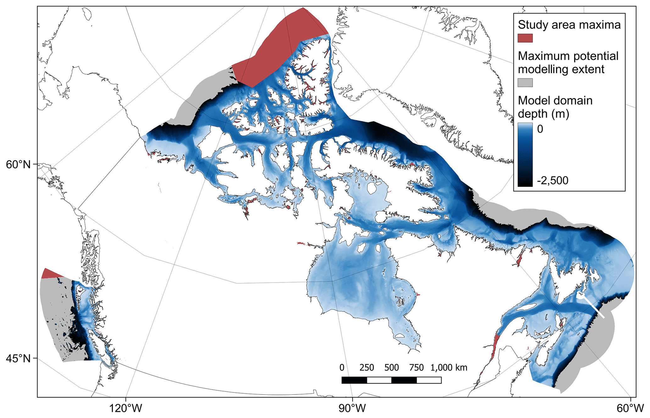
Figure 1Map of the Canadian Exclusive Economic Zone (EEZ). The study area's spatial maxima (red) were defined using the best available bathymetry data and cover the entire sub-tidal portion of the Canadian EEZ (see the high-resolution figure for further details around the coastline and Sect. 2.1.1 for more details). This is overlain by the maximum potential modelling extent (grey), which indicates only those areas where data were present for all the predictor variables (see Sect. 2.1.7). Due to the distribution of available response data, the final modelling domain was limited to a depth of 2500 m (see Sect. 2.4) and is indicated with the colour relative to the estimated depth, from 0 (light blue) to −2500 (black). Country outlines from World Bank Official Boundaries, available at https://datacatalog.worldbank.org/search/dataset/0038272 (last access: 16 May 2023).
2.1 Predictor variables
2.1.1 Bathymetry
Best available contiguous digital elevation model (DEM) data were combined and unified to a 200 m × 200 m equal-area grid covering the Canadian EEZ (coordinate reference system (CRS) EPSG:3573 – WGS 84 – North Pole Lambert Azimuthal Equal Area Canada) (Table 1; see Appendix A2 for further details). Data were filtered to contain only sub-tidal areas (those cells with elevations of less than or equal to 0 m), with the resultant extent defined as the study area spatial maxima (Fig. 1).
Table 1Summary of the predictor variables constructed for the Canadian EEZ. For more information on the methods used to derive these layers, see Sect. 2.1.
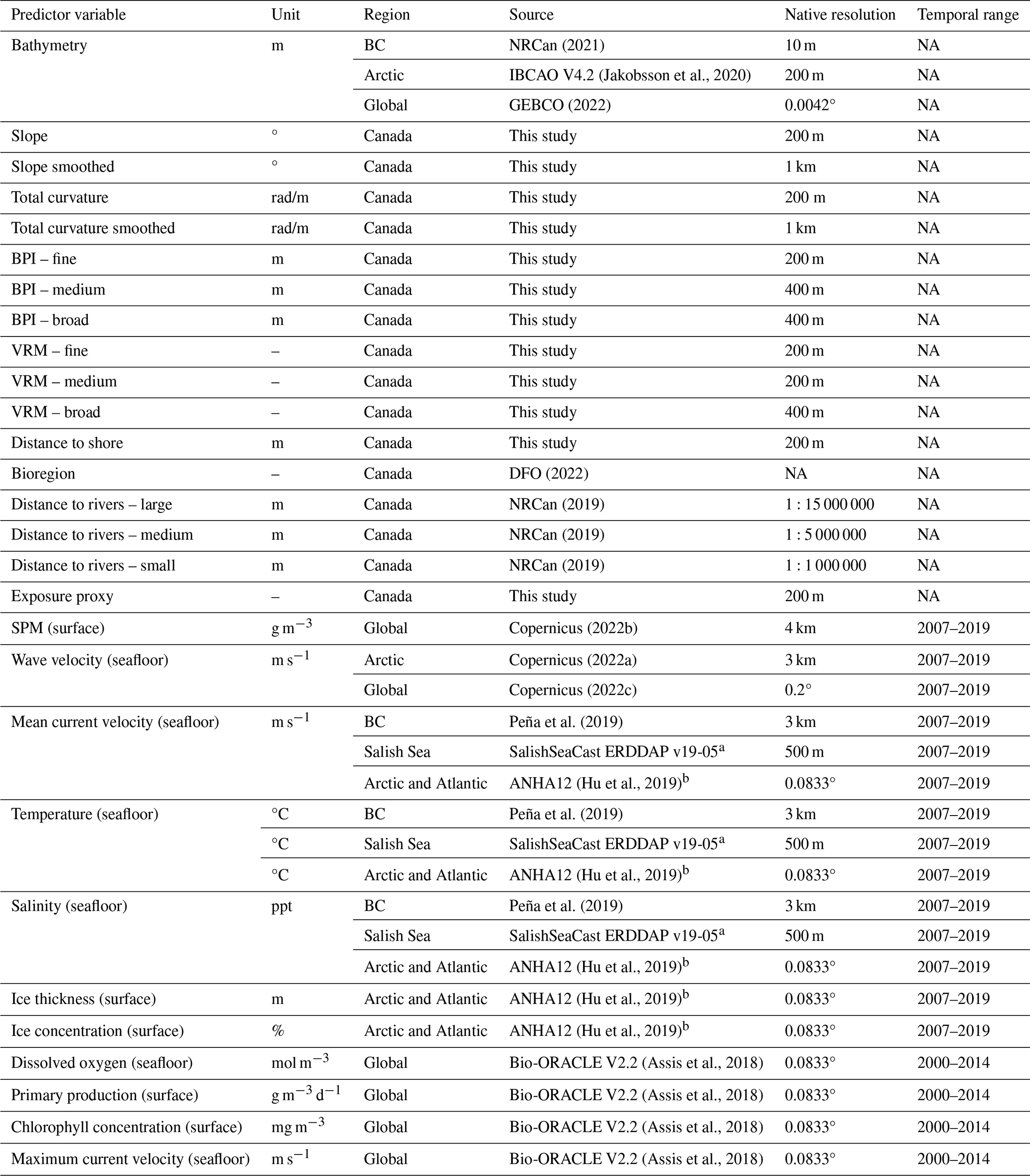
Notes: BC: British Columbia; BPI: benthic position index; VRM: vector ruggedness measure; SPM: suspended particulate matter. a See https://salishsea.eos.ubc.ca/erddap/index.html (last access: 1 February 2023), Soontiens and Allen (2017) and Soontiens et al. (2016). b See https://canadian-nemo-ocean-modelling-forum-community-of-practice.readthedocs.io/en/latest/Institutions/UofA/Configurations/ANHA12/index.html (last access: 1 February 2023). NA – not applicable
2.1.2 Benthic terrain features
A set of 10 benthic terrain features were constructed from the unified bathymetric layer (Table 1). As benthic terrain measures use data on the depth of a location relative to the depth of surrounding cells up to a given distance, bathymetric data within a given buffer outside the study area maxima were included as needed to avoid edge effects in each terrain feature. Slope and total curvature were calculated using the terra.terrain (Hijmans, 2022) and spatialEco.curvature (Evans and Murphy, 2021) functions respectively. As these measures can be particularly sensitive to artifacts from the DEMs and projections, they were constructed at two resolutions – the native 200 m resolution and, after aggregating the bathymetry 5-fold, 1 km × 1 km (termed “smoothed”). Smoothed layers were disaggregated back to a 200 m resolution to maintain uniformity across predictor layers.
Benthic position index (BPI) and vector ruggedness measure (VRM) were each calculated using the MultiscaleDTM package at three different levels to capture both small local features and larger spatial variation in terrain (Maxwell and Shobe, 2022; Ilich et al., 2021). Benthic position index was calculated as the difference between the depth of a focal cell and the mean of cells contained in annulus-shaped windows of 0.2 to 5 km (BPI fine), 2 to 25 km (BPI medium) and 4 to 100 km (BPI broad). Vector ruggedness was measured by considering variation in the depth surrounding each cell within square windows of widths 1 km (VRM fine), 5.8 km (VRM medium) and 11.6 km (VRM broad). Due to extremely inhibitive computational times when calculating VRM broad, BPI medium and BPI broad at 200 m resolution, for these features the bathymetric layer was first aggregated to 400 m resolution before feature calculation and then disaggregated back to 200 m to maintain uniformity.
2.1.3 Predictors describing the geographic setting
The geographic setting of each cell was described by its distance to the shore and rivers, its broad bioregional classification and a proxy measure for exposure describing the degree of exposure vs. shelteredness (Table 1). The geographic setting features are also influenced by the values of the surrounding pixels, and therefore appropriate buffers were also applied to the processing of these layers to avoid edge effects. The distance to the shore was measured by the Euclidian distance to the nearest land cell (indicated by an “NA” value in the bathymetry layer), while “bioregion” was defined by the Fisheries and Oceans Canada Federal Marine Bioregions classification (DFO, 2022). The bioregion polygons were edited to include all bathymetry cells and re-classified with an integer scale of 1 to 12 from east to west.
CanVec is a digital cartographic reference product produced by Natural Resources Canada (NRCan) which includes the locations of rivers across Canada at three mapped scales (NRCan, 2019). Firstly, the coarsest-scale data (1:15 000 000) were projected onto the CRS of the bathymetry layer and converted from polylines to a 2 km resolution raster. A 2 km buffer was added around each river to ensure overlap of river mouths with the bathymetry data. The resultant raster layer was resampled onto the bathymetry raster, and the grid distance of each bathymetry cell to the nearest river-mouth cell was calculated using the terra.gridDist function (Hijmans, 2022). This was then repeated for the medium-scale (1:5 000 000) and fine-scale (1:1 000 000) layers with each river raster overlain with the previous coarser-scale layer to ensure all the rivers were included as the scales decreased.
To approximate the exposure setting of each cell, data on the mean distance from the shore of the surrounding cells were used to construct a proxy value of fetch. Using the terra.focal function (Hijmans, 2022), the mean distance to the shore of the surrounding pixels was calculated in square windows of widths 10, 20, 50, 100, 175 and 250 km. Due to extremely inhibitive computational times when calculating these values at the two largest distances, the distance to the shore layer was first aggregated to 400 m resolution before focal calculations of these components and then disaggregated back to 200 m to maintain uniformity. The maximum value in each layer was then set to the relative window size and all data in each layer normalised between 0 and 1. The mean of all the layers was then calculated, which resulted in a continuous measure of relative exposure or shelteredness ranging from 0 (highly sheltered) to 1 (highly exposed).
2.1.4 Satellite-derived predictors
Using data from the Copernicus Marine Data Store, two layers were created, approximating the mass of suspended particulate matter in surface waters and the orbital velocity of waves at the seafloor. Data on suspended particulate matter (SPM) in surface waters across Canada from 2007 to 2019 were extracted in netCDF format from the ACRI-ST (Sophia Antipolis, France) company's global Bio-Geo-Chemical products at 4 km spatial resolution and monthly temporal resolution (Copernicus, 2022b). The climatological mean across this entire period was then calculated for each cell and the netCDF converted to a raster for further processing. Due to the complex nature of the Canadian coastline and the large disparity in the spatial resolution of the satellite data product (4 km) and the layers created above (200 m), the satellite raster layer was allowed to extrapolate by one cell in its native resolution by taking the mean value of neighbouring pixels. This allowed better overlap of satellite layers with the study area maxima at the coastline but limited over-extrapolation. The raster layer was then re-projected to the equal-area CRS and resampled onto the bathymetry layer using cubic-spline interpolation. Due to a lack of consistent SPM data recorded in the northern Arctic Basin, this portion of the data layer was manually removed within QGIS.
To calculate the estimated orbital velocity of waves at the seafloor, two satellite wave data products were combined with the unified bathymetry layer as constructed above. Hourly data from 2007 to 2019 at the significant wave height (Hs; VHM0) in metres and the primary wave swell mean period (Tz; VTM01_SW1) in seconds were extracted from the 0.2° resolution Global Ocean Wave Reanalysis (WAVERYS) produced by Mercator Océan International (Copernicus, 2022c) and the 3 km resolution Arctic Ocean Wave Hindcast produced by MET Norway (Copernicus, 2022a). All data were processed as the SPM data layer (except for a lack of removal of the Arctic Basin data) and converted to an estimate of orbital wave velocity at the seafloor (Urms; m s−1) using the following equation from Soulsby (2006):
where g is the acceleration due to gravity (9.806 m s−2) and d is the water depth (m), taken as the unified bathymetry layer multiplied by −1 and all values less than 1 m depth rounded up to the nearest metre (as needed for the above calculation). The resultant Arctic orbital velocity data layer was then bias-corrected to the global orbital velocity data layer utilising the qmap package with quantile mapping using a smoothing spline (Gudmundsson et al., 2012). Finally, the two data layers were overlain with the regional Arctic data, taking priority over the global data where available.
2.1.5 Ocean circulation model predictors
To incorporate the best available regional evidence, data on the mean surface ice cover, seafloor salinity, temperature and current velocity were collated from three different ocean circulation model products covering different regions of Canada (Table 1; see Appendix A3 for further details). Three-dimensional data for salinity, temperature, u velocity (eastward) and v velocity (northward) were extracted from each model, and the climatological mean across all the time points between 2007 and 2019 was calculated. For each horizontal cell, data were only retained from the lowest vertical cell within a given position (i.e. the cell which makes contact with the seafloor). Individual model outputs were then converted to spatial point data using the cell centroid positions and transformed to the unified CRS. Point data were then converted to rasters with the respective resolution of each model and the mean value taken if two points from the same model lay within a single raster cell as an artifact of reprojection. As the Arctic–Atlantic model (ANHA12) has a varying horizontal resolution, point data were rasterised using the smallest resolution of the original model (1.6 km) and then interpolated using the gstat package (Gräler et al., 2016) and a nearest-neighbour interpolation method (including cells for land within the original model grid to suppress extrapolation). For all three models, the mean current velocity was then calculated as the root mean square of the u-velocity and v-velocity values in each cell. Finally, as carried out for the satellite data layers, each raster was allowed to extrapolate by one cell at its native resolution (or for the case of the ANHA12 model – its median resolution) and was resampled onto the 200 m bathymetry grid using cubic-spline interpolation. The three rasters were then combined with data only being assigned to the spatial extent of the respective bioregions as defined in Sect. 2.1.3. Although this means that different model products were used to measure the same predictor variable in different regions, which can create biases, the bioregion predictor variable was included as a co-variate in all the models which included the ocean circulation variables, thus allowing for interactive effects and accounting for differences in circulation model structures. Combining different models can also create edge effects. However, the Arctic–Atlantic model is entirely spatially distinct and so contains no edges in common with other models. The only significant edge between the remaining two models lies at the mouth of the Juan de Fuca Strait, and minimal disparity was seen (with the other common edge occurring in the narrows of Johnson Strait).
Predictor layers describing the mean concentration and thickness of sea ice for the same temporal period across the Arctic and Atlantic were also derived from the ANHA12 model. Processing of model data and spatial rasters was conducted as above, except that a value of zero ice concentration and thickness was applied to all cells across the British Columbian Pacific bioregions.
2.1.6 Global model predictors
Four additional predictor variables were derived from Bio-ORACLE version 2.2, a global unified marine environmental data-layer collation, which gives climatological mean values at degree resolution, for 2000–2014 and a wide range of environmental variables (Assis et al., 2018). Although these datasets are of a lower resolution when compared with the regional data used above, based on previous research, there were some additional variables not available from the regional circulation models which were considered potentially important for carbon modelling (Diesing et al., 2021; Atwood et al., 2020). Three described the oceanographic chemistry and biology – i.e. primary production and chlorophyll content of the surface water column and dissolved oxygen concentration at the seafloor. The fourth predictor was an additional measure of current velocity (maximum current velocity), which was selected on top of the previously derived mean values because current velocity has been identified as a particularly strong predictor within previous seafloor sediment composition and carbon content predictive mapping studies (Gregr et al., 2021; Diesing et al., 2021; Mitchell et al., 2019). Raster data were downloaded from the Bio-ORACLE website and processed as the satellite data layers (i.e. allowed to extrapolate by one cell at its native resolution by taking the mean value of neighbouring pixels, reprojected to the unified equal-area CRS and resampled to the unified 200 m grid using cubic-spline interpolation).
2.1.7 Final collation of predictor variables
The resulting 28 predictor variable raster layers were combined into a single raster stack and any cells containing NA values removed, leaving only those cells which contained values across all the predictor layers. The remaining cells covered 92.3 % of the sub-tidal zone of the Canadian EEZ and delineated the maximum potential modelling area (Fig. 1). The final predictor variable layers are shown in the Supplement.
2.2 Sediment mud content data
Empirical point data on the seabed sediment mud content across the Canadian EEZ were extracted from two sources (Enkin, 2024; NRCan, 2022) (see Appendix A4 for further information). Data were only retained if they originated from within the top 30 cm of the sediment and had associated geographic position information (latitude–longitude coordinates; lat–long). Data were further filtered by excluding those where the sum of mud, sand and gravel content was greater than 102 % and lower than 98 % – to allow for rounding errors but to exclude invalid data. Data were also excluded if samples or sub-samples were not present from at least the top 1 to 5 cm below the sediment surface within a given sampling event. After data filtering, the mean percentage of mud was taken across replicates or sub-samples, leaving a single value for each sampling event. We chose to concentrate on sediment mud content as this has previously been identified as the key sediment composition component from a number of related carbon mapping studies (Smeaton et al., 2021; Diesing et al., 2017, 2021; Pace et al., 2021; Wilson et al., 2018). Finally, mud content data were projected onto the CRS of the predictor layers and only retained where overlap occurred. This led to a final dataset of 19 730 samples (Fig. B1).
2.3 Organic carbon content data
2.3.1 Organic carbon data collation and extraction
Data on the percentage organic carbon content (%OC) within dried surface sediments were collected from three different structured searches. Firstly, a systematic literature review was conducted through Web of Science and Scopus. Both searches were conducted on 21 September 2022. Within Web of Science, its “Core collection” was searched via the field “Topic”, which examines a paper's title, abstract, author, keywords and “keywords plus”. Within Scopus, the search was run via the field “Title-Abs-Key”, which scans a paper's title, abstract and keywords. Within both databases, the same search string was used.
(``organic carbon'' OR ``organic matter''
 OR ``organic content'' OR TOC OR
TOM) AND (coast* OR sea* OR ocean* OR estuar*
 OR marine OR gulf) AND
(sediment* OR mud* OR sand* OR clay* OR silt*
 OR gravel* OR seabed) AND
Canad*
All articles identified from the searches were exported into a single Zotero library with duplicates removed, leaving 1581 results. Screening was conducted via a hierarchical process that first assessed the title, then the abstract and finally the full text. At each stage an article was assessed against the inclusion criteria described below, with those considered relevant or of unclear relevance passing to the next level of assessment.
The inclusion criteria were defined as a (1) study conducted on sub-tidal seabed sediments (those concerning rock, shale or fauna were not included); (2) physical samples collected using a seabed sediment sampling device (e.g. cores or grabs – sediment-trap samples were not included); (3) samples from within the Canadian EEZ; (4) studies concerning the chemical composition of the sediment; and (5) organic carbon content (%) directly measured after separation of organic and inorganic components (e.g. by acidification). After the title-screening stage, 242 articles remained, followed by 123 remaining after abstract screening and a final set of 49 articles left for data extraction after review of the full text. Four additional primary literature papers were added based on expert advice. This included two large data collation studies, one concentrating on the Arctic (CASCADE; Martens et al., 2021) and one having a global scope (MOSAIC v2; Paradis et al., 2023).
The second structured search was conducted on the Canadian Federal Science Libraries Network – a repository which contains departmental publications, reports and datasets from seven science-based Canadian government departments. The search was carried out on 7 November 2022 using the same search string as for the primary literature and querying all the fields. The search led to only 178 results, and therefore each result was assessed individually against the selection criteria, first by their abstract and then by a full-text assessment, leading to data extraction from 15 reports. The third search was carried out on 15 November 2022 using GEOSCAN – the NRCan bibliographic database for scientific publications. As GEOSCAN does not allow search strings containing “AND”, the search was conducted on all the fields using only the terms “organic carbon” OR “TOC” OR “OC”, leading to 655 search results. The metadata of all the entries were exported as a text file and further refined using a secondary manual search for the remainder of the search terms listed above within Microsoft Excel. This led to a final set of 233 results, 178 of which were excluded by screening of the title and a further 51 excluded by abstract or full-text screening, leaving 4 reports for data extraction.
In total, these three structured searches of the primary literature and government reports led to 72 publications for data extraction. In addition to data on the %OC, metadata extracted included the maximum depth of the sample into the sediment (cm), geographic position (lat–long), sample ID, year of sampling (approximated as the publication year where not clearly stated), sampling method (e.g. multicorer, Van Veen grab) and water depth of the sample site (where recorded). Data were extracted on the mean %OC within each sample; however, when available, data on the %OC in different depth-layer sub-samples through a single core sample up to 50 cm were also recorded. Data were extracted from data tables or Supplement databases when available; otherwise, the PlotDigitizer online application was used to extract data from graphical products.
In addition to data collated through the structured searches, %OC data were also extracted from PANGAEA – a global data repository for geographic Earth system data (PANGAEA®, 2022). A data search across all the topics was conducted on 25 October 2022 using the same search terms as for the structured search, except for removal of the term “Canad*”. The geographic extent of the results was instead delineated using the spatial tool within PANGAEA which allows results to be filtered by the geographic coordinates of a square or rectangular extent. Overall, this led to a total of 1489 potential datasets. All relevant data within these datasets were exported using the Data Warehouse Download tool within PANGAEA. Based on expert knowledge, two additional PANGAEA datasets were added to the output from published global %OC data syntheses (Atwood et al., 2020; Seiter et al., 2004). Lastly, where the date of the sample was not recorded, the sampling year was manually added by further exploring the metadata or cited studies. To align the PANGAEA data with the systematic review data, PANGAEA data points were excluded if (1) they lacked data on %OC, (2) if they lacked metadata on the depth of a sample within the sediment, (3) if the sample originated from greater than 50 cm below the sediment surface, or (4) if metadata on the elevation or water depth indicated sampling above the sub-tidal zone. Additionally, metadata within PANGAEA were coalesced where necessary (due to different names being given to the same data type) and mean values of %OC taken if replicates were measured within a single sub-sample.
All organic carbon data were converted to spatial point data transformed to the unified equal-area CRS and masked by the predictor variable's maximum model area to leave only overlapping data. Additionally, values were only retained from the sampling year 1959 and onwards. The extra year was included when compared with the mud content data because there were some wide-scale surveys undertaken across the Labrador Sea in 1959, which was lacking from any additional %OC datasets. While this large temporal extent may add uncertainty in relation to the quality and uniformity of the response data, similar extents have been used by previous global mapping studies (Atwood et al., 2020; Lee et al., 2019; Seiter et al., 2004), and 72 % of the %OC data within this study were sampled after 1980 and 55 % after 2000. The larger temporal extent also allows for the inclusion of a higher frequency and a wider spatial extent of data, thereby potentially improving the robustness of our spatial predictive models. In total, our %OC dataset contained 2518 point samples (Fig. B2) and 3308 sub-samples across different depth layers within cores.
2.3.2 Organic carbon data processing
Due to commonly adopted uneven sampling distributions within single core samples (i.e. more sub-samples towards the top of the core), where sub-sample data were present in the %OC at different depth layers, these were converted to weighted cumulative means assuming a linear distribution between sub-samples. Additionally, there was large variation in the maximum sediment depth of point samples, ranging from %OC measures from only the top 1 cm of sediment to values up to the chosen data extraction limit of 50 cm deep. We chose to standardise all samples to 30 cm depth as only 6 % of the point samples covered sediment depths below this layer and because 30 cm is a commonly suggested carbon stock accounting depth for terrestrial soil and marine sediment habitats in both carbon-accrediting methodologies and greenhouse gas inventories (VERRA, 2020; IPCC, 2019).
To estimate the cumulative mean of %OC at 30 cm for all the individual point samples, we created a transfer function using a generalised additive mixed-model (GAMM) smoothing spline. It is generally expected that the %OC in marine sediments will decrease with depth within the seafloor (Middelburg, 2018); we used the collated data above to approximate a mean trend for this study. Firstly, only those data that contained at least five sub-sampled depth layers were retained for modelling, as fitting distributions to those with fewer points would likely be invalid. This left 183 unique samples with 2640 weighted cumulative mean sub-samples for model construction. Cumulative mean %OC data were arcsin-transformed (arcsin, a commonly adopted transformation for percentage data) and a simple GAMM applied with sub-sample sediment depth as the fixed factor modelled with a cubic regression spline and a sample ID as the random factor. The GAMM was fitted using the mgcv package, a scaled t-distribution family was used for heavy-tailed Gaussian-like data, the number of basis dimensions was set to 20, and smoothing parameter estimation was conducted by restricted maximum likelihood (REML) (Wood et al., 2016). Model validation was carried out using visual assessment of diagnostic plots of residuals as well as observed vs. fitted values. The significance of the sampling depth smoothing spline was assessed by an analysis of variance (ANOVA) with a chi-squared test comparing the full GAMM to a null GAMM containing only the random factor and the intercept (see Appendix C for the results). The difference between the estimated deviances explained in the full and null models was also used to approximate the variance explained by the fixed and random factors. To create a transfer function, the cumulative %OC was predicted from the mean fixed effects of the GAMM at sediment depths from 0 to 30 cm at 0.1 cm intervals. The predictions were then back-transformed to percentage data, and the cumulative mean %OC at each depth was converted to an inverse proportion of the mean across 30 cm. Overall, this gave an estimated proportional conversion factor from the cumulative mean at any given depth to an expected mean across 30 cm (Appendix C).
All point-sample data from PANGAEA and the systematic review were combined, corrected to weighted cumulative means where sub-samples were present, checked for duplication, and unified to a mean %OC value of the top 30 cm of sediment using the above transfer function. One outlier was removed from the dataset as it was reported to have a carbon content twice that of any other sample within the dataset. Finally, for further analyses, %OC data were arcsin-transformed due to a highly right-skewed distribution and its application within similar modelling exercises (Smeaton et al., 2021; Diesing et al., 2017).
2.4 Final model domain selection
After visual assessment of the coverage of both the mud content and %OC data, the final model domain was limited to a water depth of 2500 m. This depth limit (as delineated by the bathymetry predictor layer) encompassed 99.95 % of the mud content point data (Fig. B1) and 99.3 % of the %OC data (Fig. B2). The predictor layer raster stack was filtered with all cells deeper than 2500 m excluded from the model domain. This final model domain covers 4 489 235 km2, which is 78.4 % of the EEZ or 92.6 % of the seafloor area above 2500 m (Fig. 1).
2.5 Random forest modelling
For predictive mapping, we adopted random forest machine learning techniques due to their flexibility regarding violations of traditional statistical assumptions, ability to handle a range of data types and predictor variables and elucidate both drivers of model response and predictions of uncertainty, as well as their successful application in previous similar modelling tasks (Diesing et al., 2017, 2021; Pace et al., 2021; Atwood et al., 2020; Wilson et al., 2018). Mud content and %OC were both modelled using the following framework. Firstly, each response variable was overlain onto the predictor variable grid and the mean values were taken if more than one data point fell within a single raster cell. All predictor variable data were then extracted for each response dataset; however, the three biological and biochemical predictor variables (primary production, chlorophyll concentration and dissolved oxygen) were only used within the %OC model as they are not expected to drive variation in physical sediment properties (Restreppo et al., 2021; Gregr et al., 2021; Graw et al., 2021; Mitchell et al., 2019).
Contemporary research in spatial machine learning techniques has highlighted that robust spatial cross-validation (CV) strategies and predictor variable selection processes are essential for calculating valid performance metrics, limiting overfitting and constructing reliable spatial predictions (Zhang et al., 2023; Ludwig et al., 2023; Meyer and Pebesma, 2022; Meyer et al., 2019). Details of the methods used to ensure appropriate cross-validation design and feature selection are discussed in Appendix A5. For both response variables, following identification of an appropriate 35-fold spatial CV structure, a single fold was held back as testing data, with all other data retained for model training. To ensure an absence of duplication between the training and testing data, 34 spatial CV folds were reconstructed on the training data (i.e. all training data assigned to 1 of 34 validation sets). Using these CV folds, the CAST.ffs function (Meyer et al., 2023) was then used to run forward predictor variable selection processes with appropriate spatial considerations (see Appendix A5 for further information).
Following variable selection, hyperparameter tuning was conducted on the hyperparameters mtry (the number of variables to randomly sample as candidates at each split) and min_n (the number of observations needed to keep splitting nodes), with the trees hyperparameter (the number of random forest trees to construct and take mean predictions across) set to 1000 (Probst et al., 2019). Eleven potential combinations of hyperparameters were selected using a semi-random Latin hypercube grid (Kuhn and Silge, 2023; Kuhn and Wickham, 2020). The tuning process fitted separate models across all the CV folds and hyperparameter combinations (i.e. 34 CV folds multiplied by 11 hyperparameter options gives a total of 374 models) (Kuhn and Silge, 2023; Kuhn and Wickham, 2020). The performance of each of the 11 hyperparameter combinations was assessed by calculating the root mean squared error (RMSE) in predictions of the validation data across all the CV folds, with the optimal hyperparameter combination selected as that with the lowest RMSE (Meyer et al., 2019, 2023). After selection of the best-performing hyperparameter combination, a single last-fit model was constructed on the entire training set and evaluated on the held-back test set (Kuhn and Silge, 2023; Kuhn and Wickham, 2020), with the absence of overfitting determined by the RMSE and R2 of the last-fit model falling within the range of those found across CV folds with optimal hyperparameters. The final model performance metrics (RMSE and R2) were then calculated using all predictions of validation data from CV folds (with optimal hyperparameters) and using predictions of the testing data from the last-fit model (Meyer et al., 2019, 2023). Predicted values were then calculated across the entire model domain using the last-fit model and the predictor variable raster stack (Kuhn and Silge, 2023; Kuhn and Wickham, 2020), and cell-specific estimation of uncertainty was calculated using the standard error in out-of-bag predictions using an infinitesimal jackknife for bagging (Roy and Larocque, 2020; Wager et al., 2014). Due to computational restraints when calculating predictions across the entire model domain (which contains 112 230 871 cells), the predictor variable raster stack was split into 150 non-overlapping partitions by random sampling and both prediction and standard error estimates made serially on each partition. All the predictions were then merged to create a raster layer covering the entire model domain (although edge effects were not expected between partitions, random sampling without replacement across the entire domain was chosen to ensure its absence).
A cell-specific approximation of the upper and lower bounds of the 95 % confidence interval (CI) was calculated by adding or subtracting the cell-specific standard error estimates, each multiplied by 1.96, from the mean predictions and then back-transformed where needed (Kuhn and Wickham, 2020; Wager et al., 2014). After calculation, CI values were corrected where necessary – being bounded by 0 and 100. The resulting three raster layers from the mud content model were also used as available additional predictor variables when constructing the random forest models for %OC (Fig. 2). Although this gives the potential for data leakage if mud content and %OC data were from the same samples, we found only 31 occurrences (1.3 % of the OC samples) where direct spatial overlap occurred, and therefore we do not consider significant data leakage to be present and no impact on variable importance or model performance calculations will be seen. Finally, a measure of relative predictor variable importance was calculated by fitting an additional single random forest model on all training data using optimal hyperparameters, and the predictor importance was calculated on out-of-bag data through permutation of predictor variable values (for further details, see Kuhn and Silge, 2023; Wright et al., 2016). Accumulated local effect (ALE) plots for the last-fit model were produced for the six predictor variables with highest importance in each model using the iml package (Molnar et al., 2018) to give a visual representation of the average effect of predictors on model prediction outcomes.
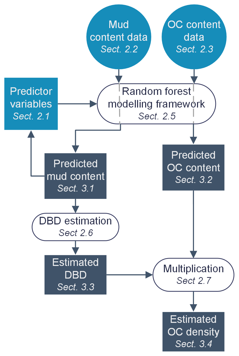
Figure 2Study workflow diagram. Outline of the structure and linkages within the proceeding Methods and Results sections. Light-blue shapes indicate input data, white ovals indicate data processes, dark shapes indicate output data, rectangles indicate raster data, and circles indicate point data. OC: organic carbon; DBD: dry bulk density.
2.6 Estimating sediment dry bulk density
An estimate for the dry bulk density of the sediment (ρD – the mass of dried sediment per unit volume within the seafloor; g cm−3) was constructed across the model domain based on the predictions of mud content from the random forest model (Fig. 2). We identified three published functions which describe the relationship between mud content and porosity (Φ; the proportion of sediment volume which is water) in seabed sediments. The following equations are respectively from Jenkins (2005), Diesing et al. (2017) and Pace et al. (2021).
Due to each of these equations being approximations of the relationship between mud content and Φ, we chose to take the mean response. In all the equations, mud represents the predicted mean mud content values as calculated above, each expressed as a decimal proportion. For Eq. (4), mud content was rounded up to the nearest 0.01 as lower values give unrealistic porosity estimates. Sediment porosity can then be converted to an estimate of dry bulk density using the following equation:
where ρS is the grain density of seabed sediments (g cm−3), which was set at the frequently used constant approximation of 2.65 (Diesing et al., 2017, 2021; e.g. Pace et al., 2021; Lee et al., 2019; Wilson et al., 2018; Kuzyk et al., 2017). Although this standard approximation of grain density is not ideal, the variation under different environmental settings is generally found to be small when compared with differences in %OC and porosity. Therefore, the values of grain density are not expected to strongly drive variation in organic carbon density (Atwood et al., 2020; Lee et al., 2019; Middelburg, 2019; Martin et al., 2015; Berner, 1982).
To incorporate uncertainty from our mud content predictions, estimates of dry bulk density were also calculated from the cell-specific predictions of the lower and upper bounds of the 95 % CI of mud content. We used these derived lower and upper bounds of dry bulk density estimates as best available approximations of uncertainty around the dry bulk density mean estimate values. Equivalent approaches to estimating uncertainty have been used in other seabed sediment carbon mapping studies (e.g. Diesing et al., 2017, 2023; Lee et al., 2019).
2.7 Estimating organic carbon standing stock
The organic carbon density (g cm−3) is calculated by multiplying the %OC (expressed as a decimal proportion) by the sediment dry bulk density (Fig. 2). For the final calculations, the respective means and upper and lower uncertainty bounds were multiplied together to incorporate uncertainty from both components. These compound uncertainties were used as the best available approximations of the lower and upper bounds of uncertainty around the estimates of mean organic carbon density (akin to Diesing et al., 2017, 2023; Lee et al., 2019). To create a more meaningful response value, organic carbon density was converted (kg m−3; multiplied by 1000). Finally, the organic carbon stock in each mapped cell can be calculated by multiplying the organic carbon density by the reference sediment depth of this study (0.3 m) and the cell area (40 000 m2) and converted to metric tonnes (divided by 1000). Overall, this allows estimates to be calculated for the total values of organic carbon stock across different parts of the model domain.
2.8 Rock substrate distribution case studies
The method followed in this study is similar to that used for many similar seabed sediment predictive mapping exercises in that it uses data only from sediment grab and core samples to build predictive maps across the model domain (Restreppo et al., 2021; Graw et al., 2021; Diesing et al., 2017, 2021; LaRowe et al., 2020a; Atwood et al., 2020; Lee et al., 2019; Mitchell et al., 2019; Wilson et al., 2018; Stephens and Diesing, 2015). One major limitation with this modelling approach is that areas of bedrock, which would have zero values for all sediment response variables, will not be recorded in these datasets. Therefore, the underrepresentation of zero values in the response data could lead to an overestimation of organic carbon standing stocks as zero values are unlikely to be predicted from model outputs.
In the context of this study, information regarding the distribution of bedrock is lacking for many regions. We therefore use two regional case studies from the Pacific British Columbian EEZ and the Atlantic Scotian Shelf and slope where recent publications have made estimated maps of the distribution of rock substrates (Philibert et al., 2022; Gregr et al., 2021). Each of these products was overlain on the final spatial predictions of sediment carbon densities and all cells set to zero where rock substrates were predicted. The proportional effect on the mean, upper and lower estimates of carbon stock was then calculated in each bioregion.
3.1 Mud content predictive mapping
Of the 25 predictor variables available for mud content random forest modelling, 13 were selected in the optimal model (Fig. 3). The mean orbital velocity of waves at the seafloor and the mass of suspended particulate matter at the surface were the variables with the highest importance (Fig. 3). Other variables with relatively high importance for predicting mud content included the exposure setting, ice thickness, distance to rivers, bathymetry and benthic position indices (Fig. 3). A higher mud content was generally predicted in areas of low wave velocity, low exposure and closeness to but not directly adjacent to river mouths, with the effect of SPM and ice thickness less distinct, likely due to more complex interactive effects (Fig. 4).
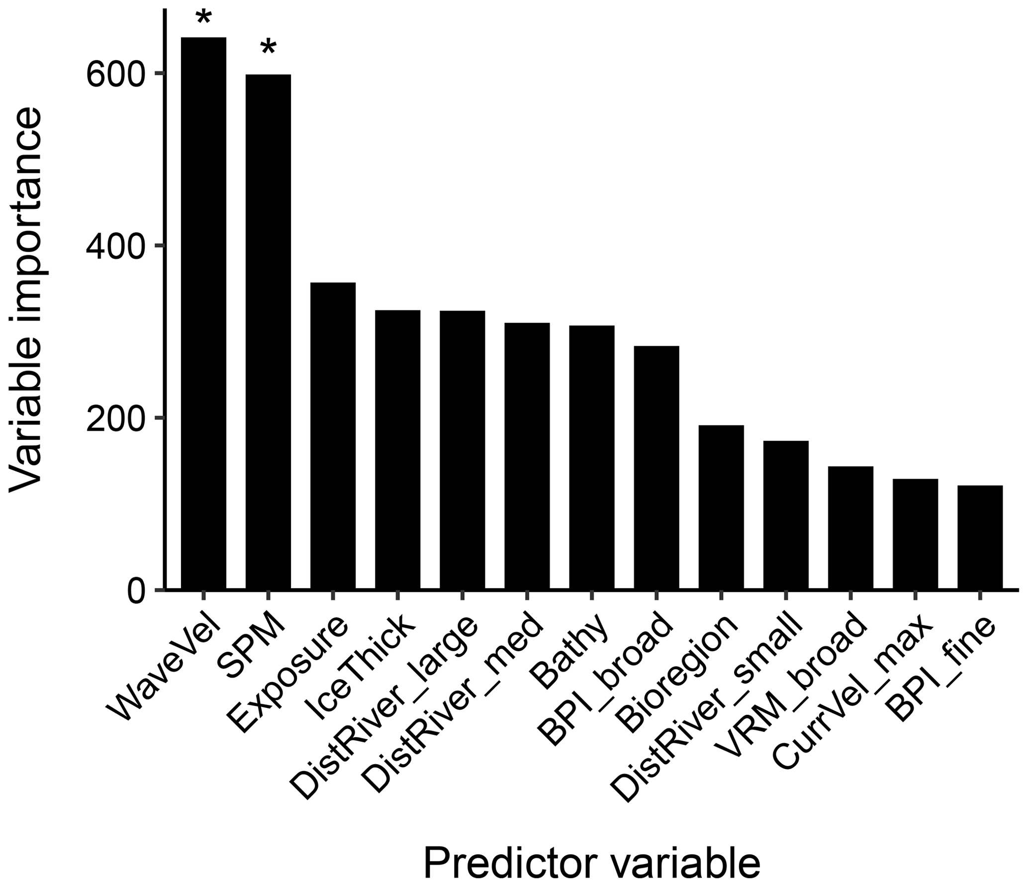
Figure 3Predictor variable importance from random forest models of mud content in marine sub-tidal sediments. The y axis is a unitless relative variable importance score for each model. Asterisks indicate the two initial predictors which were selected based on variable importance, with all the other predictor variables selected using a forward-selection process (see Appendix A5 for further details). WaveVel: orbital wave velocity at the seafloor, SPM: suspended particulate matter within the water column, BPI: benthic position index, DistRiver: distance to the nearest river, IceThick: sea ice thickness, Bathy: bathymetry, VRM: vector ruggedness measure, CurrVel: current velocity at the seafloor.
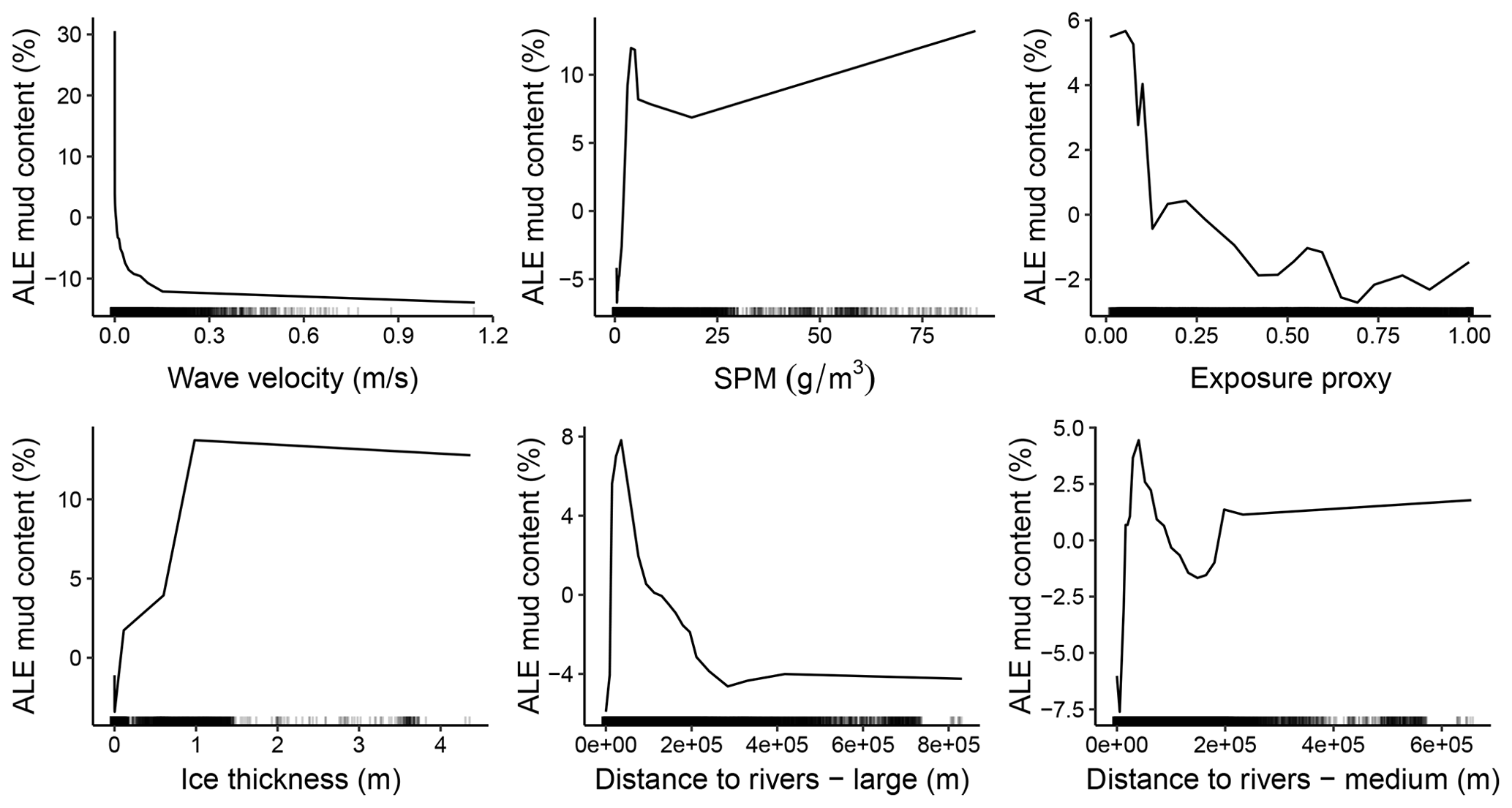
Figure 4Accumulated local effect (ALE) plots for the six predictor variables with the highest importance in the mud content random forest model. ALE (distributions drawn with lines) gives a visual representation of the average effect of the predictor variable on the response but does not indicate the influence of multi-way interactions which are inherent in random forest models. Rug plots (dashed marks at the bottom) indicate the distribution of each variable within the training dataset.
Areas with sediments dominated by mud (> 75 %) were predicted across the basins of many of the Pacific fjords, inlets and estuaries and within the southern Salish Sea (Fig. 5). In the Arctic, mud-dominated areas included large parts of the Canadian western Arctic as well as Hudson Bay. In the Atlantic, the Laurentian Channel and deeper parts of the Scotian Shelf contained particularly high mud fractions (Fig. 5). Across the model domain, sediment in deeper areas on the continental slope was also highly dominated by mud (Fig. 5). Using robust spatial cross-validation, the model was estimated to have an RMSE of 24.4 % and R2 of 0.60. The cell-specific upper and lower 95 % CI bounds are shown in Fig. E1. On average, the upper CI bounds were 28 % larger than the mean and the lower CI bounds 20 % less.
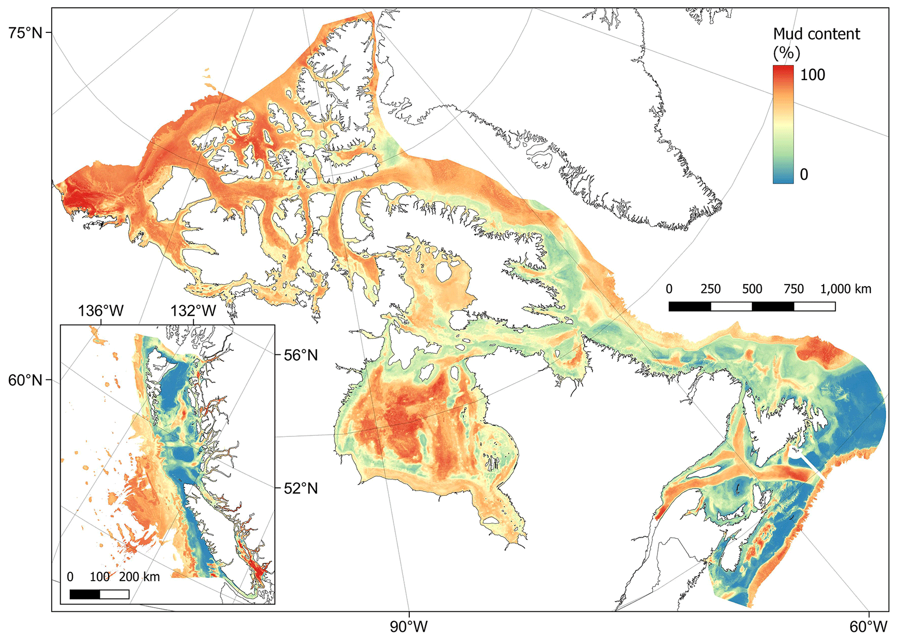
Figure 5Predictive mapping of mud content (%) in sub-tidal marine sediments across the Canadian continental margin. The main plot shows the Arctic and Atlantic regions with the Pacific region inset. The 95 % confidence interval bounds around the predicted means are shown in Fig. E1. Labels indicating the locations of different areas mentioned within the text are shown in Fig. B3. Country outlines from World Bank Official Boundaries, available at https://datacatalog.worldbank.org/search/dataset/0038272 (last access: 16 May 2023).
3.2 Organic carbon content predictive mapping
Eleven predictor variables were selected in the optimal %OC model (Fig. 6). The variables with the highest importance in predicting %OC were the mud content layers constructed above (specifically the mean and the lower bound), with all other predictors having less than half the relative importance of the mean mud predictions (Fig. 6). On average, organic carbon content increased with predicted mud content and was generally higher in areas with low SPM concentrations and low exposure settings, close to but not directly adjacent to rivers and at high water temperatures (Fig. 7).
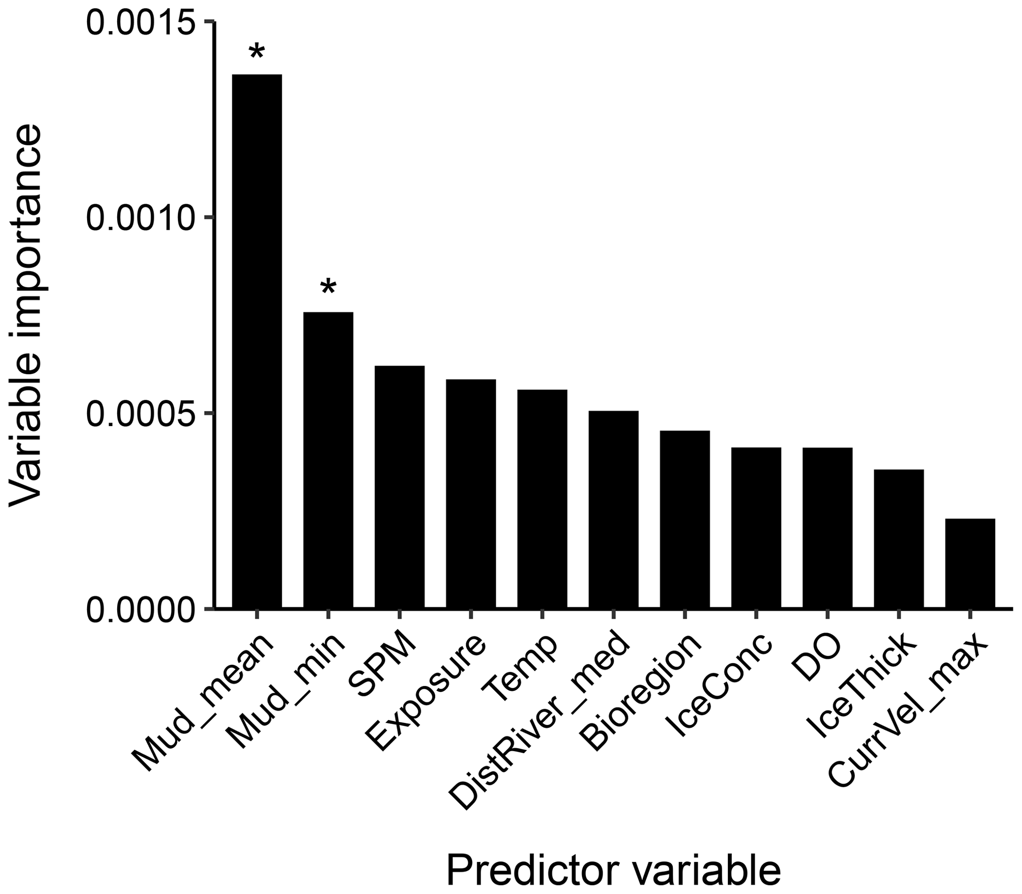
Figure 6Predictor variable importance from random forest models for the organic carbon content in marine sub-tidal sediments. The y axis is a unitless relative variable importance score. Asterisks indicate the two initial predictors which were selected based on variable importance, with all other predictor variables selected using a forward-selection process (see Appendix A5 for further details). Mud_min: lower bound of 95 % CI for mud content, SPM: suspended particulate matter within the water column, Temp: temperature, DistRiver: distance to the nearest river, IceConc: sea ice concentration, DO: dissolved oxygen at the seafloor, IceThick: sea ice thickness, CurrVel: current velocity at the seafloor.
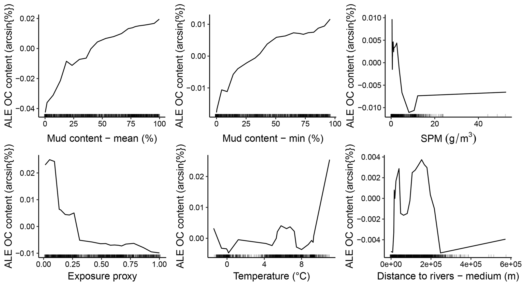
Figure 7ALE plots for the six predictor variables with highest importance in the organic carbon (OC) content random forest model. ALE (distributions drawn with lines) gives a visual representation of the average effect of the predictor variable on the response but does not indicate the influence of multi-way interactions which are inherent to random forest models. Rug plots (dashed marks at the bottom) indicate the distribution of each variable within the training dataset.
The predictions of %OC ranged from to 5.6 %, with an overall mean of 0.8 ± 0.3 % (± SD). Areas with the highest predicted %OC (> 3 %) were restricted to parts of the Pacific West Coast fjords and channels and small parts of the inlets and bays on the eastern coast of Nova Scotia and around Passamaquoddy Bay in the Bay of Fundy (Fig. 8). High concentrations (i.e. > 1 %) were more widespread across these areas and covered much of the Beaufort Sea, western Baffin Bay and Foxe Basin in the Arctic, southern and central Hudson Bay, the Laurentian Channel, coastal northern Newfoundland and the central Scotian Shelf in the Atlantic, as well as the Salish Sea and deeper areas to the south of the British Colombian Pacific continental margin (Fig. 8). The lowest %OC was predicted across shallower parts of the central Pacific shelf and near coastal areas west of Vancouver Island (Fig. 8). Cross-validation estimated an R2 for the model of 0.58 and an RMSE of 0.09 arcsin{%OC}. Cell-specific upper and lower 95 % CI bounds are shown in Fig. E2. On average, the upper CI bounds were 42 % larger than the mean prediction and the lower CI bounds 33 % less than the mean prediction.
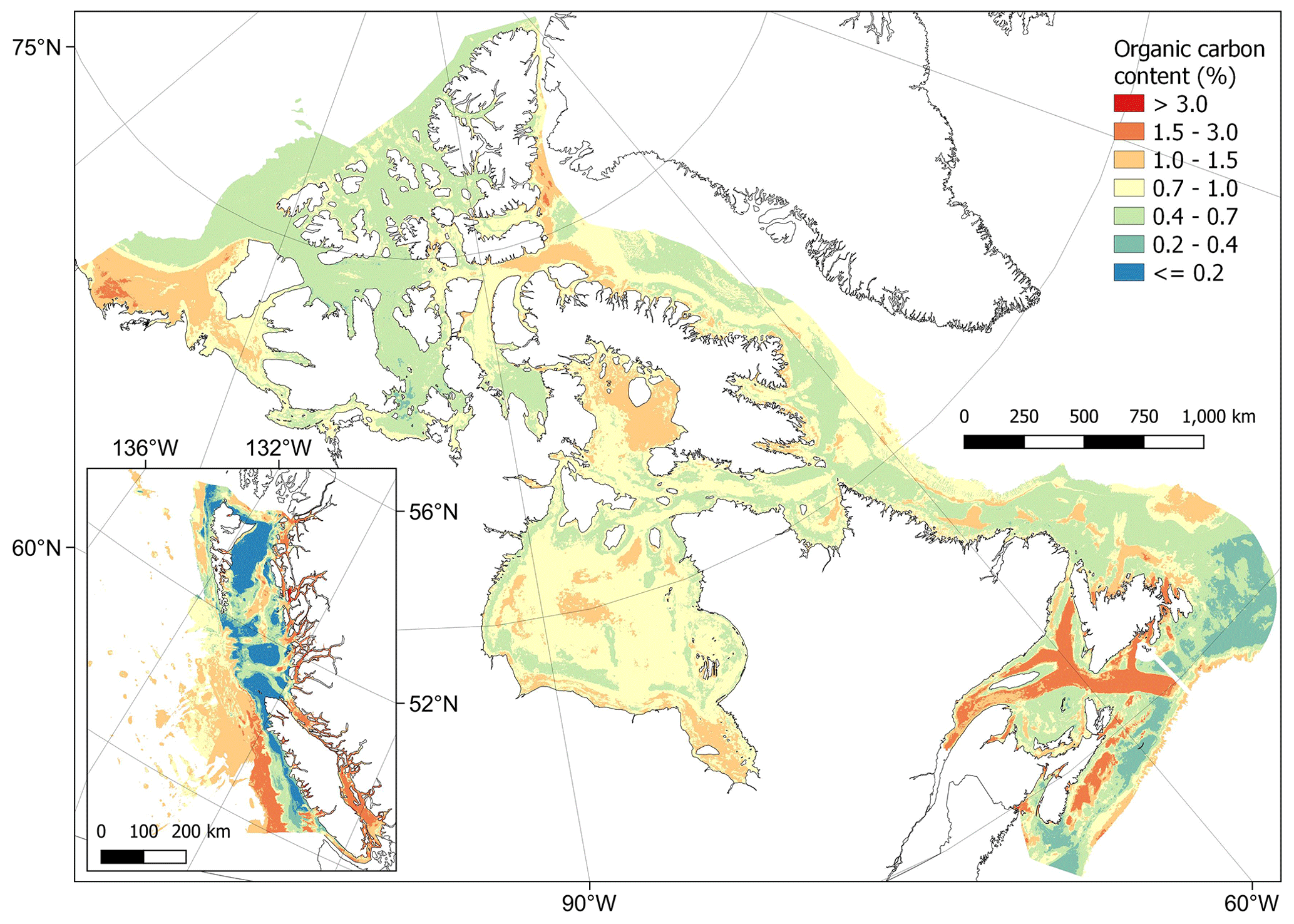
Figure 8Predictive mapping of organic carbon content (%) in sub-tidal marine sediments across the Canadian continental margin. The main plot shows the Arctic and Atlantic regions with the Pacific region inset. The continuous variable is shown displayed in discrete colour bands to improve visualisation of highly right-skewed data. The 95 % confidence interval bounds around the predicted means are shown in Fig. E2. Labels indicating the locations of different areas mentioned within the text are shown in Fig. B3. Country outlines from World Bank Official Boundaries, available at https://datacatalog.worldbank.org/search/dataset/0038272 (last access: 16 May 2023).
3.3 Dry bulk density estimation
The dry bulk density of sediments was estimated using the predicted values of mud content from our random forest model and previously published functions for conversions to porosity and dry bulk density (Fig. 2). Estimated values ranged from 0.67 to 1.61 g cm−3 with a mean of 1.04 ± 0.21 g cm−3 (± SD). As expected from its derivation, the spatial distribution of the dry bulk density values was very similar to the mud content values predicted above (Fig. 5). That is, the lowest dry bulk density was estimated in mud-dominated areas (Fig. 9). Cell-specific upper and lower uncertainty bounds are shown in Fig. E3. On average, these bounds were 6.2 % larger and 6.0 % lower than the cell-specific mean estimate.
3.4 Estimated organic carbon density and standing stock
From combining predictions of dry bulk density and organic carbon content, organic carbon density could be estimated across the Canadian continental margin (Fig. 2). Estimated values ranged from to 58.4 kg m−3 with a mean of 8.1 ± 2.8 kg m−3 (± SD). Spatial patterns in organic carbon density (Fig. 10) were similar to those found for organic carbon content (Fig. 8). Areas with the highest carbon density (> 25 kg m−3) were restricted to small areas within near-shore zones, including inlets and fjords of British Columbia (Pacific), as well as enclosed near-shore areas of the Atlantic East Coast (Fig. 10). High carbon densities (> 15 kg m−3) were predicted to occur across wide parts of these areas as well as further offshore in parts of the Laurentian Channel and central Scotian Shelf and at the edge of the continental slope off the west of Vancouver Island (Fig. 10). In the Arctic, areas with relatively high carbon (> 10 kg m−3) were predicted across many near-shore areas as well as across large parts of the Beaufort Shelf, Foxe Basin, James Bay and Kane Basin (Fig. 10). Cell-specific upper and lower uncertainty bounds are shown in Fig. E4. On average, the upper bounds were 50 % higher than the mean prediction and the lower bounds 37 % less than their means.
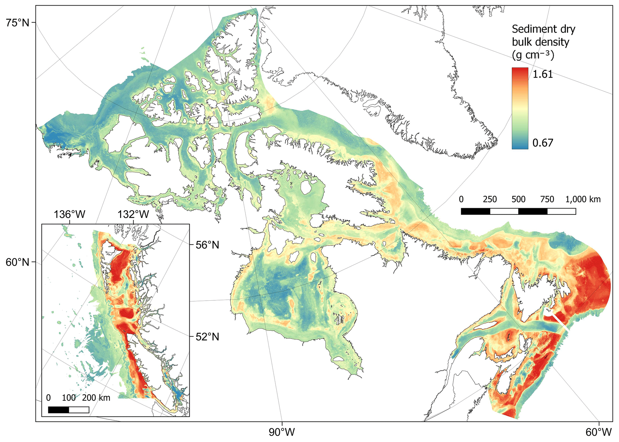
Figure 9Estimates of sediment dry bulk density (g cm−3) across the Canadian continental margin. The main plot shows the Arctic and Atlantic regions with the Pacific region inset. The estimated bounds of uncertainty around the predicted means are shown in Fig. E3. Labels indicating the locations of the different areas mentioned within the text are shown in Fig. B3. Country outlines from World Bank Official Boundaries, available at https://datacatalog.worldbank.org/search/dataset/0038272 (last access: 16 May 2023).
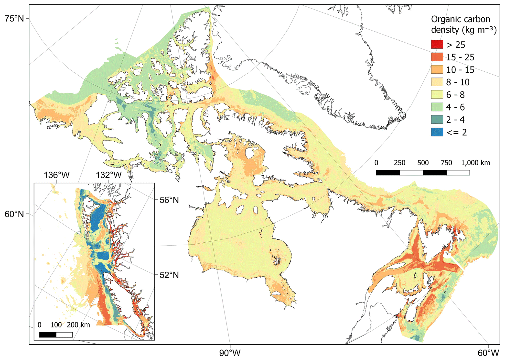
Figure 10Estimates of organic carbon density (kg m−3) across the Canadian continental margin. The main plot shows the Arctic and Atlantic regions with the Pacific region inset. The continuous variable is shown in discrete colour bands to improve visualisation of highly right-skewed data. The estimated bounds of uncertainty around the predicted means are shown in Fig. E4. Labels indicating the locations of the different areas mentioned within the text are shown in Fig. B3. Country outlines from World Bank Official Boundaries, available at https://datacatalog.worldbank.org/search/dataset/0038272 (last access: 16 May 2023).
Using a standardised sediment depth of 30 cm, the total standing stock of organic carbon in surficial sediments across the model domain is estimated at 10.9 Gt with uncertainty bounds of 7.0–16.0 Gt. Between bioregions, total stock was predominantly related to total areal extent, for example with Hudson Bay having the largest carbon stock and the largest area (Table 2). The Strait of Georgia and Southern Shelf bioregions of the Pacific had the lowest total standing stocks due to their small extent. However, by unit area, these regions contained the highest organic carbon stocks, along with the Gulf of St. Lawrence (Table 2).
Table 2Summary of estimated mean total organic carbon stocks in surficial seabed sediments of different bioregions across the Canadian continental margin. Organic carbon standing stocks are estimated for the top 30 cm of seabed sediments. For delineation of the different bioregions, see the Supplement.
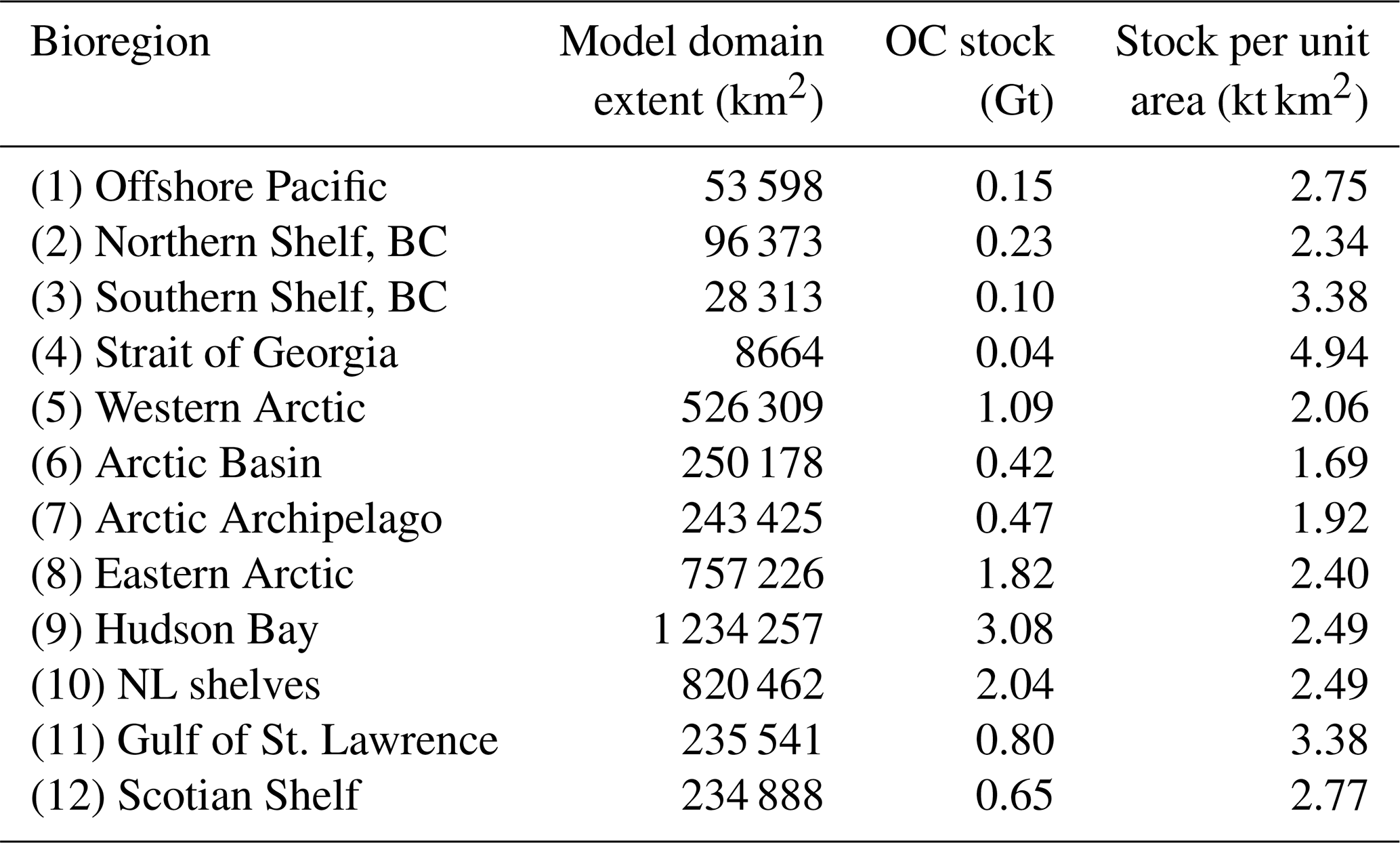
Notes: OC: organic carbon; NL: Newfoundland–Labrador.
3.5 Rock substrate distribution case studies
As the predictive maps produced in this study rely on physical sediment samples alone, they are unlikely to produce valid estimates for areas of bedrock – i.e. estimates of zero sediment carbon density where bedrock is located. On the Scotian Shelf (bioregion 12), correcting our predictive maps with a predicted bedrock distribution map (Fig. F1) reduces the total organic carbon stock estimates in this region by between 7.7 % and 7.8 %, leading to a value of 0.59 Gt (0.37–0.90 Gt). For the Pacific British Columbian marine region (bioregions 1–4), assigning zero values to areas covered by a predicted bedrock distribution map (Fig. F2) would reduce our estimates by 9.1 %–9.7 % to a total of 0.46 Gt (0.29–0.71 Gt) of organic carbon.
All the mapped products as shown in Figs. 5, 8, 9 and 10 have been made available as georeferenced TIFF files in the Borealis data repository at https://doi.org/10.5683/SP3/ICHVVA (Epstein et al., 2024). This includes the mean predictions as well as the cell-specific uncertainty bounds as shown in Appendix E. The repository also contains all data collated within the systematic data review of organic carbon content and the georeferenced TIFF files from the rock distribution case studies (Appendix F). Additionally, all the associated code used for data manipulations, model building and predictive mapping can be found in the above repository.
Using best available data, we have produced the first national assessment of organic carbon in surficial seabed sediments across the Canadian continental margin, estimating the standing stock in the top 30 cm to be 10.9 Gt (7.0–16.0 Gt). Although comparisons with previous global studies are challenging due to differences in sediment reference depths, mapping resolutions and total spatial coverage, our estimate falls within a similar range to those previously published, e.g. 2.2 Gt in the top 5 cm (Lee et al., 2019) and 48 Gt in the top metre (Atwood et al., 2020) of the Canadian EEZ. In contrast to these global studies, the national approach taken here allows for a more complete data synthesis, a finer spatial resolution, larger spatial coverage of the Canadian continental margin and spatially defined estimates of uncertainty. Similarly to other national and regional mapping studies (Smeaton et al., 2021; Diesing et al., 2017, 2021), areas of high organic carbon stocks were predominantly predicted to occur in coastal fjords, inlets, estuaries, enclosed bays and sheltered basins as well as deeper channels and troughs (Fig. 10). To put our estimated organic carbon standing stock into context, 10.9 Gt equates to 52 % of the organic carbon estimated to be stored in all Canadian terrestrial plant live biomass and detritus (both above and below ground) and 9.8 % of soil organic carbon to 30 cm across Canada (Sothe et al., 2022).
5.1 Model interpretation and uncertainties
The two key components of the carbon stock estimates in this study are the predictive maps for mud content and organic carbon content, which were estimated to have map accuracies of 60 % and 58 % respectively (R2 0.60 and 0.58). While these values may seem relatively low when compared with some other related studies (Diesing et al., 2017, 2021; Atwood et al., 2020; Mitchell et al., 2019), the use of robust, spatial cross-validation to calculate model evaluation metrics (as we did herein) has been shown to produce significantly more conservative estimates of map accuracy when compared with frequently used random cross-validation approaches (Ludwig et al., 2023; Meyer et al., 2019) such as those used in both global seabed carbon stock studies discussed above (Atwood et al., 2020; Lee et al., 2019). Within this study, we also calculated cell-specific uncertainty bounds. While there are many ways to calculate model uncertainty, thereby making comparisons between studies challenging, the uncertainty in carbon density calculated here (37 %–50 % either side of the mean) is close to those found in similar regional (Diesing et al., 2021; 58 %) and global studies (Lee et al., 2019; 49 %), both of which predict carbon stocks at significantly coarser resolutions. Our bounds for total standing stock (36 % lower and 47 % higher than the mean) are also similar to the estimated bounds from the recently published predictive models of Canadian terrestrial vegetation and soil carbon (a 90 % confidence interval of 48 % either side of the mean) (Sothe et al., 2022).
Using two case studies from British Columbia and the Scotian Shelf, we estimated that the distribution of rock substrates could reduce our estimates of carbon stock by approximately 7.7 %–9.7 % (Figs. F1 and F2). As much of the Canadian coastline is distant from significant infrastructure, extensive surveys of the seafloor are generally lacking, especially when compared with similar regional carbon mapping studies in north-western Europe (e.g. Smeaton et al., 2021). It is therefore unclear how representative these case studies are of the entire Canadian EEZ. Improved data on the presence of bedrock across less-studied regions of the Canadian Arctic, Hudson Bay, Gulf of St. Lawrence, Newfoundland and Labrador may allow for the production of a predictive map of bedrock across the Canadian EEZ which would significantly improve the carbon estimates and spatial predictive maps produced in this study.
Areas of uncertainty which could not be fully quantified include the accuracy and precision of response data and predictor layers. The response data drive the model construction, and therefore sampling, processing or recording errors can propagate into predictions. This is particularly relevant given the large temporal extent of response data which was required to gain sufficient coverage for this work (1959–2019). This long duration may also add additional variation from temporal differences between data, e.g. from differing anthropogenic drivers of carbon storage and/or accumulation (Keil, 2017). However, similar temporal extents have been used in related studies (Atwood et al., 2020; Lee et al., 2019; Seiter et al., 2004), and 72 % of the organic carbon data in this study were sampled after 1980 and 55 % after 2000. In the response data, assumptions and/or predictions were also required regarding the distribution of mud and carbon across sediment depths. While standardising for this factor is clearly necessary, especially when using a wide variety of legacy data, it does add additional uncertainty which would not be present if wide-scale standardised sampling methods were employed. The results from this study do however highlight that, within the top 30 cm of sediment, the spatial location of the sample is a far stronger driver of organic carbon content than the sediment sampling depth (Table C1).
Most of the predictor variables used in this study are also themselves modelled products that contain their own inherent uncertainties and/or interpolations which cannot be fully quantified here. Additionally, many predictors are constructed at spatial resolutions significantly coarser than those used for modelling and prediction in this study. This meant that predictor data had to be interpolated, with significant inherent assumptions regarding the variation and distribution of the data. Although best available data were used in this study, if predictor variables were available at higher native resolutions, fewer assumptions would be necessary and significant differences may be found in predictions as well as their uncertainty and variability. Many of the predictor variables also have temporal components, and while the climatological mean of a 12- to 14-year time span used in this study is expected to produce variables representative of the study region, they do not completely align with the temporal extent of the response data, which could add further prediction uncertainty. Finally, due to data availability, the uncertainty bounds around our mean estimates of dry bulk density and organic carbon density were approximated from the constructed 95 % CIs of mud content and %OC from the random forest models. While these provide an appropriate measure of uncertainty in our estimates in the context of this study, if large empirical datasets became available for dry bulk and organic carbon density, it would be preferable to construct predictive models, mean estimates and uncertainty bounds for these response variables directly.
5.2 Future directions and applications
Improvements could be made in future iterations of these sediment carbon maps when additional response data become available. The size of the organic carbon content dataset was relatively small (2518 point samples) given the size of the model domain, so new data could greatly improve accuracy and reduce uncertainty in predictions. Additionally, widespread empirical data on sediment dry bulk density would reduce the assumptions needed to use approximate conversions from mud content, while a large geographically dispersed empirical dataset on seabed sediment organic carbon density (i.e. where OC content and dry bulk density are measured directly in each physical sample) would reduce assumptions even further, with the potential to construct a single predictive map for this response alone (Diesing et al., 2021). There are also improvements to be made with the development of higher-resolution or more accurate predictor layers. This would be particularly relevant for those variables with coarse resolutions and those which were seen to have the highest importance in our models or related seabed sediment mapping studies (e.g. Gregr et al., 2021; Diesing et al., 2017, 2021; Mitchell et al., 2019), i.e. wave velocities, suspended particulate matter, exposure, current velocities and oxygen concentrations. Further validation and refinements could also be supported by numerical biogeochemical modelling products where the organic carbon densities are mathematically estimated based on oceanographic, climatological and benthic conditions, including the potential to incorporate predictions in different future climate scenarios (Ani and Robson, 2021).
The organic carbon predictive mapping product generated here could have many future applications. Regionalisation and prioritisation processes could identify key areas of carbon storage for further research and possible protections (Epstein and Roberts, 2022, 2023; Diesing et al., 2021). There is also potential to combine these mapped products with spatial data on human activities occurring on the seafloor to consider potential management implications, such as controlling the levels of impactful industries (e.g. mobile bottom fishing, mineral extraction or energy generation) in areas with high organic carbon (Clare et al., 2023; Epstein and Roberts, 2022). The mud content predictive maps may also have wider applications for marine planning, being a strong driver of the biological habitat type and sensitivity. Overall, these data have wide-scale relevance across the marine ecology, geology and environmental management disciplines. However, the use of these products should always consider the discussed uncertainties and quantified uncertainty bounds of predictions. As with all large-scale mapping exercises, continued empirical data collection is needed for improved accuracy of mapping seabed carbon stocks across Canada.
A1 Analysis software
Analyses were primarily undertaken in R 4.2.2 (R Core Team, 2022) and Rstudio 2022.12.0.353 (Posit Team, 2022), with some additional data manipulation and spatial plotting in QGIS (QGIS.org, 2021) and Python (Van Rossum and Drake, 2009). Within R, raster data were handled using the terra package (Hijmans, 2022), spatial vector data used the sf package (Pebesma, 2018), netCDF data used the stars (Pebesma and Bivan, 2023) and tidync (Sumner, 2022) packages, data frames used the dplyr package (Wickham et al., 2019), and vector data used base R (R Core Team, 2022). Random forest modelling was primarily dependent on the ranger package (Wright and Ziegler, 2017). However, models were constructed and tuned using the tidymodels package (Kuhn and Wickham, 2020), with cross-validation and predictor variable selection using the CAST (Meyer et al., 2023) and caret (Kuhn, 2008) packages. Plotting utilised the above packages as well as ggplot2 (Wickham et al., 2019) and patchwork (Pedersen, 2022), while parallel processing used the doParallel package (Microsoft Corporation and Weston, 2022).
A2 Bathymetry layer construction
To define the maximum potential spatial coverage of this study, best available bathymetric datasets were combined across the Canadian EEZ (Table 1). Firstly, three DEM raster layers covering different extents of the Canadian EEZ were each filtered to contain only those elevations of less than or equal to 0 m. Where necessary, data were then aggregated (averaged) or disaggregated (split) to a resolution of approximately 200 m, and all the layers were projected onto a unified 200 m × 200 m equal-area grid CRS (EPSG:3573 – WGS 84 – North Pole Lambert Azimuthal Equal Area Canada). Reprojection was necessary as all three DEMs were in different coordinate systems, including some already being projected. The 200 m resolution was chosen as it is the median native resolution of the three DEMs while also being considered towards the upper limit of what may be computationally possible within the scope of this study. After reprojection, the three layers were overlain, with the region-specific data given priority over the global data where present. Finally, the seaward boundaries were delineated by the outer extent of the Canadian EEZ (Flanders Marine Institute, 2019).
A3 Details of ocean circulation models
ANHA12 is a regional configuration of the NEMO ocean and sea ice model (Madec et al., 1998) created at the University of Alberta, covering the Arctic and Northern Hemisphere Atlantic at 5 d temporal resolution, a curvilinear degree horizontal resolution ranging from 1.93 km in the Arctic to 9.3 km at the Equator, and 50 vertical levels (Hu et al., 2019). The British Columbian continental margin (BCCM) circulation model created by Fisheries and Oceans Canada (DFO) covers the entire Canadian Pacific coast and extends approximately 400 km offshore. It has a uniform horizontal resolution of 3 km, 42 vertical levels and a 3 d temporal resolution (Peña et al., 2019; Masson and Fine, 2012). As the BCCM model has higher uncertainty in near-shore and enclosed environments due to its relatively coarse resolution, data were also extracted for the enclosed Salish Sea from the Salish Sea Cast ERDDAP data server. Similarly to ANHA12, the Salish Sea Cast is a configuration of the NEMO circulation model developed by a consortium of Canadian universities and government agencies and extends from Juan de Fuca Strait to Puget Sound to Johnstone Strait at 500 m horizontal resolution, 40 vertical layers and hourly temporal resolution (Soontiens and Allen, 2017; Soontiens et al., 2016). For further details on all these models, see the relevant cited references. It should be noted that many of these ocean circulation models contain high uncertainty in near-shore areas. However, they are expected to be greatly improved when compared with global circulation model products (Peña et al., 2019; Hu et al., 2019; Soontiens and Allen, 2017), which are frequently used in this sort of predictive mapping work (e.g. Atwood et al., 2020; Lee et al., 2019; Assis et al., 2018).
A4 Sediment grain size data collation and processing details
Sediment composition point data were extracted from two sources. Firstly, all data were exported from the NRCan Expedition Database on 11 November 2022. This data repository contains information related to marine and coastal field surveys conducted by or on behalf of the Geological Survey of Canada from the 1950s to the present, which deployed sampling methods including piston cores and grab samples. Data were also extracted from a recent synthesis of grain size distribution measurements from the Canadian Pacific seafloor (1951–2017), compiled by the Geological Survey Of Canada and NRCan (Enkin, 2024). Although there are some duplications between these two datasets, these are accounted for in the proceeding pre-processing steps. In both sources, grain size data are reported as the percentage content of mud (sometimes separated into silt and clay), sand and gravel within each sample. Due to modern developments in grain size analyses (e.g. laser diffraction), older samples may have lower measurement accuracy; however, due to the relatively coarse metric being used in this study (mud, sand or gravel) and the occurrence of a number of large-scale geological surveys occurring during the 1960s, we chose to retain data from 1960 onwards. When the sampling year was not recorded within the database, the date was inferred from the expedition code or from expedition metadata. The sampling method and depth of the sediment from which the sample or sub-sample originates are also predominantly recorded within the database. Where sediment depth was absent, the sampling method was noted as “grab” or “other”, and the penetration depth was assumed to be 10 cm (a commonly assumed penetration of standard sediment sampling devices such as Van Veen grabs and Day grabs).
A5 Details on the construction and implementation of spatial cross-validation and feature selection
For each response variable modelled in this study (mud content and %OC), the spatialsample package (Mahoney et al., 2023) was used to construct a variety of spatial CV data-fold structures, and the validity of each structure was visually assessed using the CAST.plot_geodist function (Meyer et al., 2023). This function creates density plots of nearest-neighbour distances (Euclidean) in multivariate predictor space (using normalised variables) between response data locations and a random sample of prediction locations and between data inside and outside each CV fold (Ludwig et al., 2023; Meyer et al., 2023; Meyer and Pebesma and Bivan, 2023). The suitability of a given CV structure to be representative of estimating map accuracy can be determined by visually assessing the density plots and finding the CV distance curve being closely aligned with the density curve of response data to prediction distances (see Appendix D; Ludwig et al., 2023; Meyer and Pebesma, 2022). To approximate response-to-prediction distances, the sample size number within plot_geodist was set to select 5000 random samples across the model domain. Further, as the spatial distribution of data is a key consideration to ensure robust cross-validation (Ludwig et al., 2023; Meyer and Pebesma, 2022), for the plot_geodist calculations alone, the x and y coordinates of each data point were included in addition to those predictor variables listed in Table 1 and described in Sect. 2.5.
For the mud content data, a spatial k-means clustering CV structure was chosen as the response data had good coverage of the model domain, contained a large number of data points, and showed relatively strong spatial clustering (Fig. B1). A range of options in the number of k-means clusters were tested, with 35 being determined as the optimal number and each cluster being assigned to its own CV fold (Fig. D1). Through visual assessment of the density plots, we identified that the k-means CV structure was somewhat misaligned from response-to-prediction distances, with the CV distances being overly conservative at including near-distance comparisons (Fig. D1). We therefore used a partially repeated CV strategy with a small number of randomly selected data points added to the assessment set in each k-means spatial CV fold (1 % of mud content data randomly sampled at each fold without replacement) (Fig. D2). As the %OC response dataset was relatively small and spatially dispersed (Fig. B2), we used a spatial block CV strategy in place of the k-means clustering to avoid clusters containing highly spatially dispersed data. We chose to use hexagonally shaped blocks, random assignment of blocks to folds and the same number of CV folds as for the mud content data (v=35) – both to maintain uniformity and because varying the fold number did not significantly influence the density plots. Instead, the diameter of the spatial blocks was altered and an optimal block size of 100 km identified using the plot_geodist function (Fig. D3).
The CAST.ffs function (Meyer et al., 2023) was used to run a forward predictor variable selection process with appropriate spatial considerations. The function fits a model with all combinations of two-way predictors, selects the best model based on a given metric, and then increases the number of predictors by 1, testing all the remaining variables. This iteratively continues with the process stopping if none of the tested variables increases the performance when compared with the best previous model with n−1 predictors. The function allows models to be fit separately on each spatial CV fold (as defined above), with the overall performance of each iteration based on model accuracy across all the CV folds. This therefore incorporates appropriate spatial considerations into the feature selection process. Due to the large number of variables within this study and the relatively large datasets, this process was very computationally expensive. We therefore chose to adapt the function to initiate forward variable selection after initial identification of the first two predictor variables. These variables were identified by constructing a single random forest model with all training data and predictor variables and the hyperparameters mtry (the number of variables to randomly sample as candidates at each split), min_n (the number of observations needed to keep splitting nodes) and trees (the number of random forest trees to construct and take mean predictions across) set to 2, 5 and 1000 respectively. Variable importance was estimated on out-of-bag samples through permutation of predictor variable values (Wright et al., 2016) and the two predictor variables with the highest importance selected. The ffs function was then run starting with the two pre-selected variables (see Figs. 3 and 6) and the performance of each iteration assessed on the root mean squared error (RMSE) of predictions across all the CV folds.
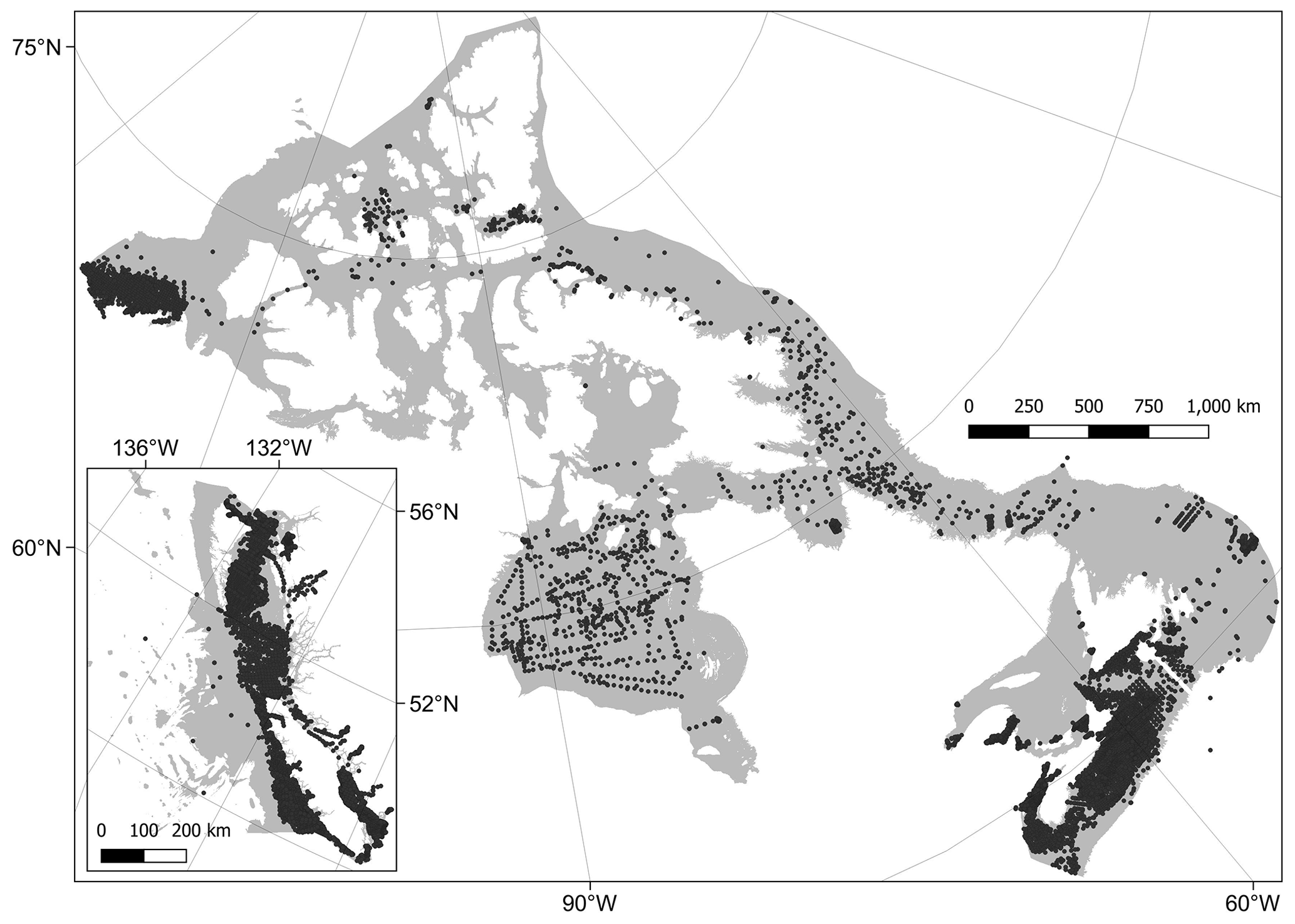
Figure B1Map showing the distribution of mud content samples across the model domain.
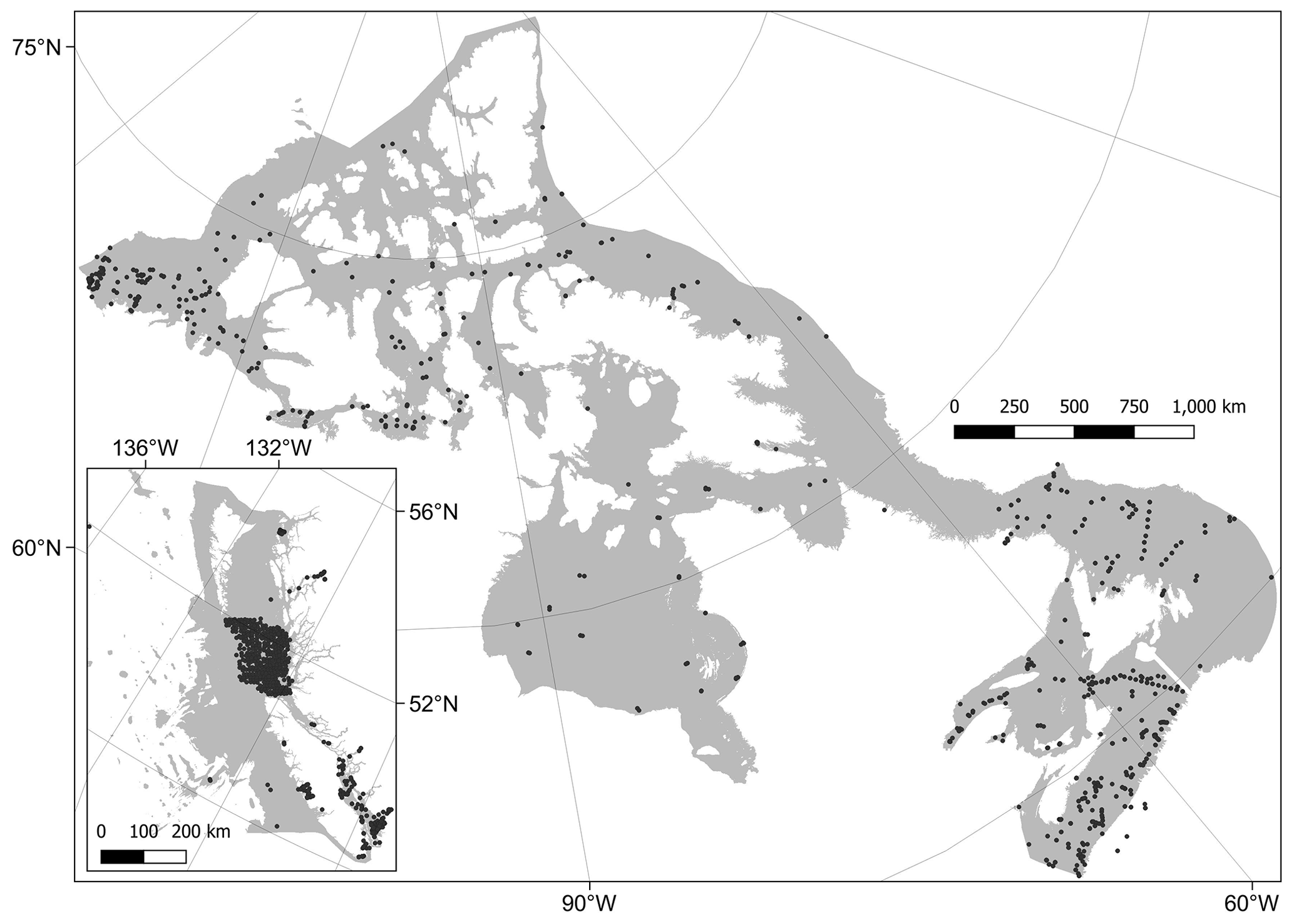
Figure B2Map showing the distribution of carbon content samples across the model domain.
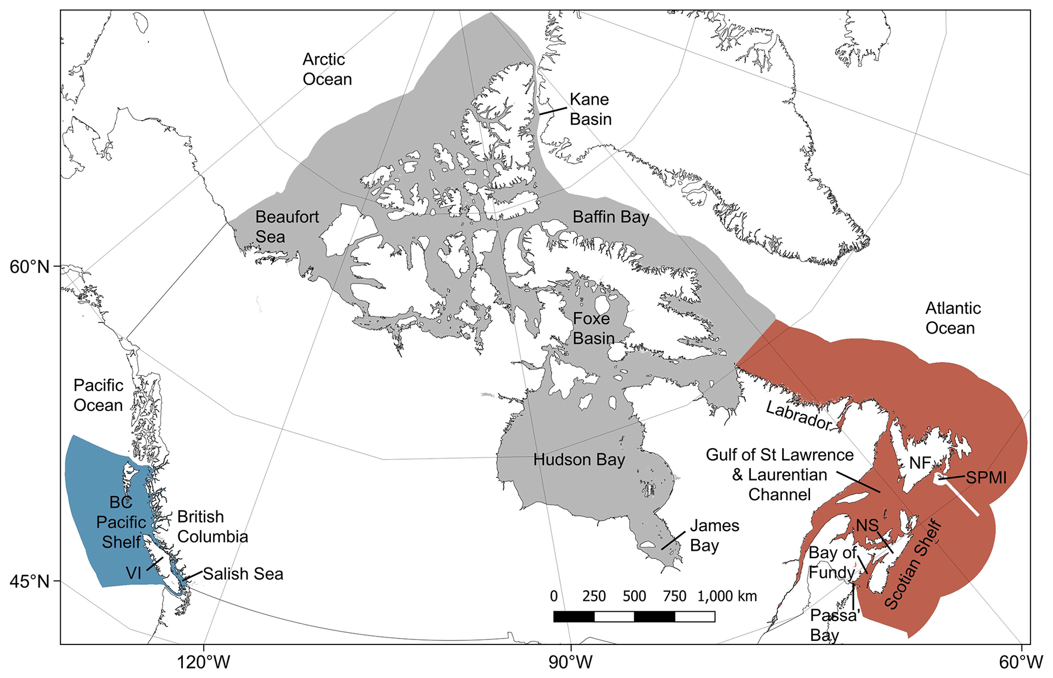
Figure B3Map indicating the locations of different areas which are mentioned within the text. The Canadian Pacific (blue), Arctic (grey) and Atlantic (red) regions are shown with labelled locations overlain. BC: British Columbia; Passa' Bay: Passamaquoddy Bay; NS: Nova Scotia; NF: Newfoundland; SPMI: St. Pierre and Miquelon. The locations are for guidance only and do not represent the entire extent or exact location of a given area. Country outlines are derived from World Bank Official Boundaries, available at https://datacatalog.worldbank.org/search/dataset/0038272 (last access: 16 May 2023).
There was a significant effect of sampling depth on the organic carbon content in seabed sediments (χ2=1400.9, p<0.001). While sample ID explained most of the variation between sub-sample carbon contents, the sampling depth was also a significant factor (Table C1). Carbon content decreased with increasing sampling depth (Fig. C1). The rate of the carbon content decline generally decreased with increasing depth into the sediment. However, uncertainty in this trend increased within deeper sediment layers (Fig. C1).
The predicted mean effect of sediment depth on carbon content was extracted from the model and converted to a transfer function which states the expected ratio between the carbon content across 30 cm compared with the cumulative mean at any given sampling depth (Fig. C2). The ratio ranged from 89.3 % when only measuring the sediment surface to 93.7 % when measuring the carbon content across the top 10 cm, and by 25 cm it was approaching equilibrium at 98.8 %.
Table C1Results from the generalised additive mixed model between the carbon content of marine sediments and the sampling depth. A basic generalised additive mixed model with a scaled t distribution was constructed for carbon content in sediment sub-samples, with sample ID as the random factor and sampling depth as the fixed factor.
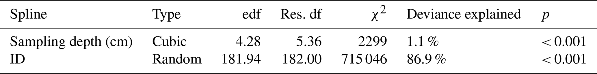
Notes: edf: effective degrees of freedom. Res. df: residual degrees of freedom.
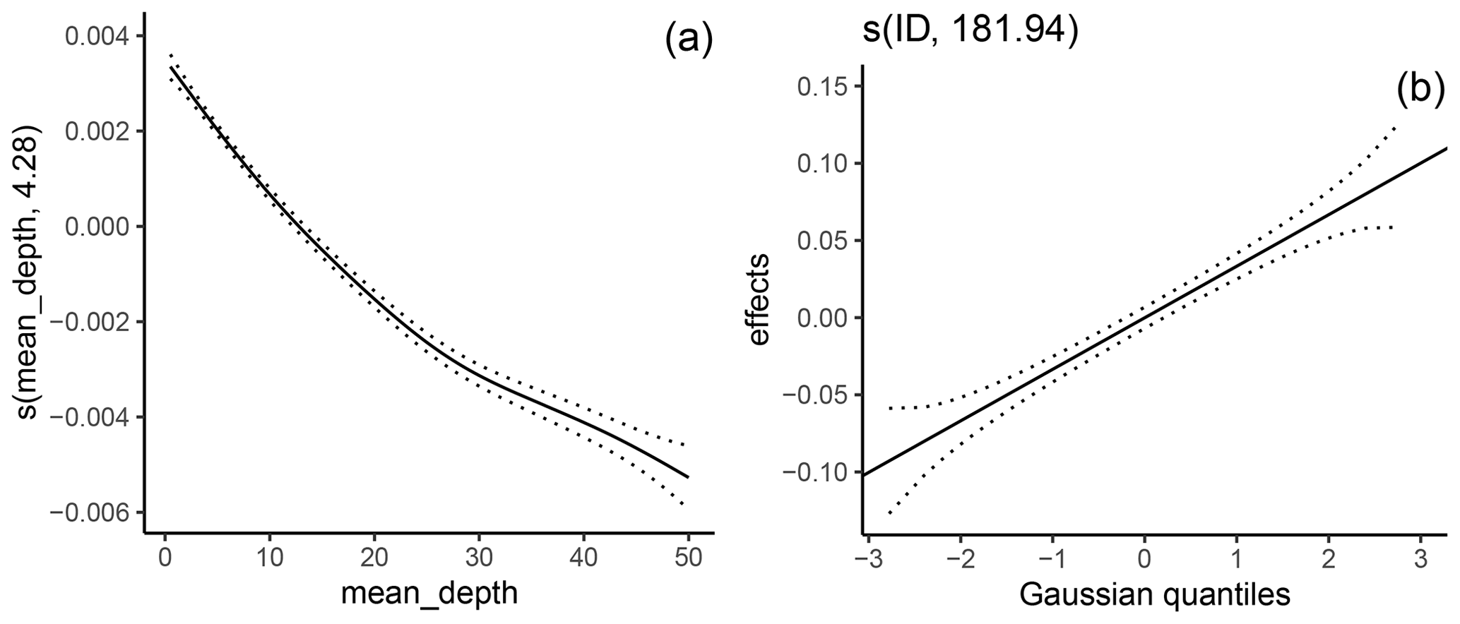
Figure C1Regression splines indicating the effect of sediment sampling depth (a) and sample ID (b) on the organic carbon content in seabed sediment sub-samples.
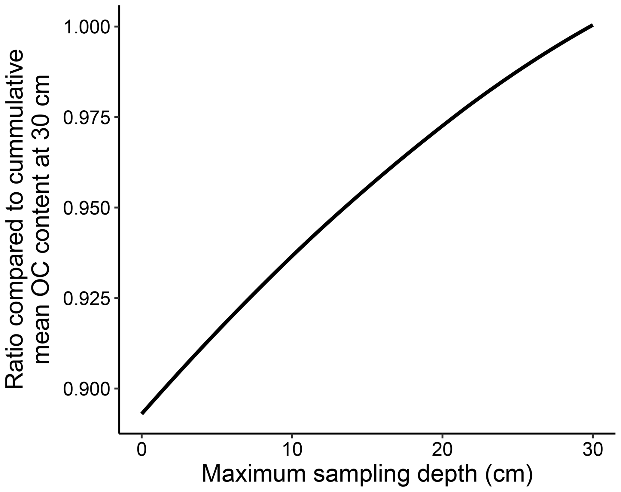
Figure C2Transfer function for cumulative mean organic carbon (OC) content at 30 cm sediment depth. Using a generalised additive mixed model, an estimated transfer function was constructed to standardise the cumulative mean carbon content at any given depth to an expected value at 30 cm.
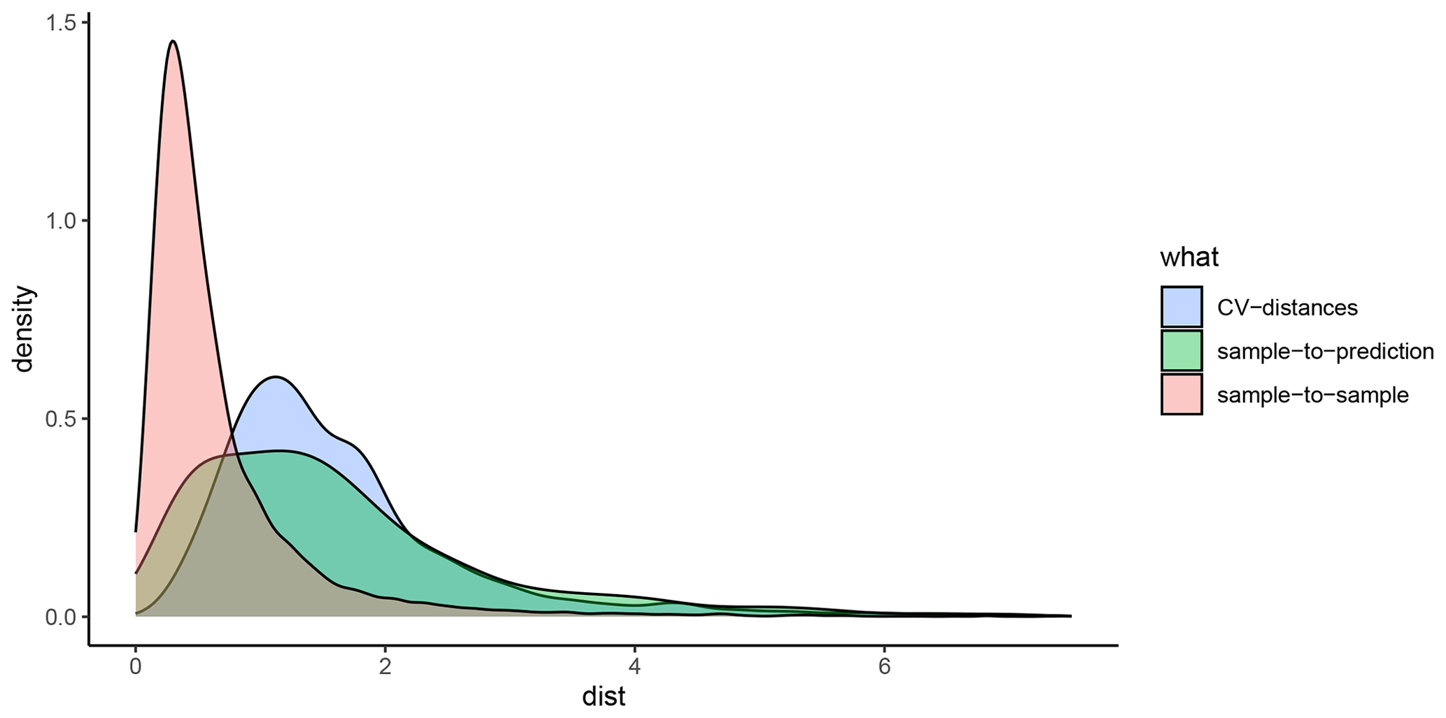
Figure D1Multivariate nearest-neighbour distance density plot for mud content data with the optimal number of spatial k-means clusters across cross-validation (CV) folds. The frequency of nearest-neighbour distances (x axis) is shown for sample-to-sample distance (red), sample-to-prediction distance (green) and CV-fold analysis-to-assessment distance (blue). dist: multivariate Euclidean distance in predictor space after normalisation of predictors. An optimal number of 35 clusters was selected due to the close overlap between the CV distance and sample-to-prediction curve.
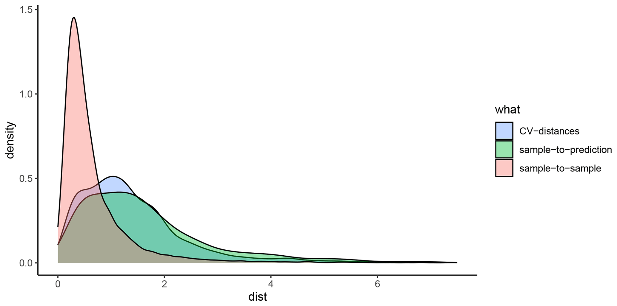
Figure D2Multivariate nearest-neighbour distance density plot for mud content data with a partially repeated spatial random mixture method for CV folds. The frequency of nearest-neighbour distances (x axis) is shown for sample-to-sample distance (red), sample-to-prediction distance (green) and CV-fold analysis-to-assessment distance (blue). Due to the optimal spatial k-means clustering showing poor overlap at lower multivariate distances (Fig. D1), a 1 % random sample without replacement was added to each fold.
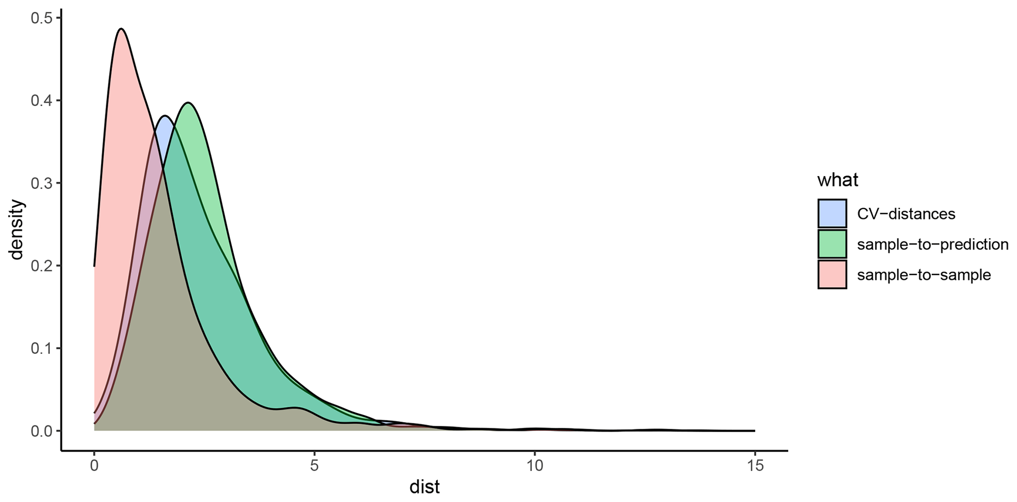
Figure D3Multivariate nearest-neighbour distance density plot for organic carbon content data with the optimal block size across CV folds. The frequency of nearest-neighbour distances (x axis) is shown for sample-to-sample distance (red), sample-to-prediction distance (green) and CV-fold analysis-to-assessment distance (blue). dist: multivariate Euclidean distance in predictor space after normalisation of predictors. An optimal block size of 100 km was selected due to close overlap between the CV distance and the sample-to-prediction curve.
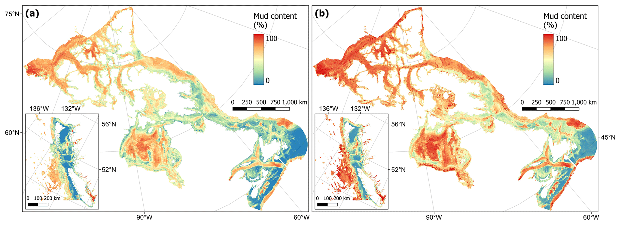
Figure E1Estimated lower (a) and upper (b) bounds of the 95 % confidence interval for predictions of mud content (%) in sub-tidal marine sediments across the Canadian continental margin. Within each panel the main plot shows the Arctic and Atlantic regions with the Pacific region inset.
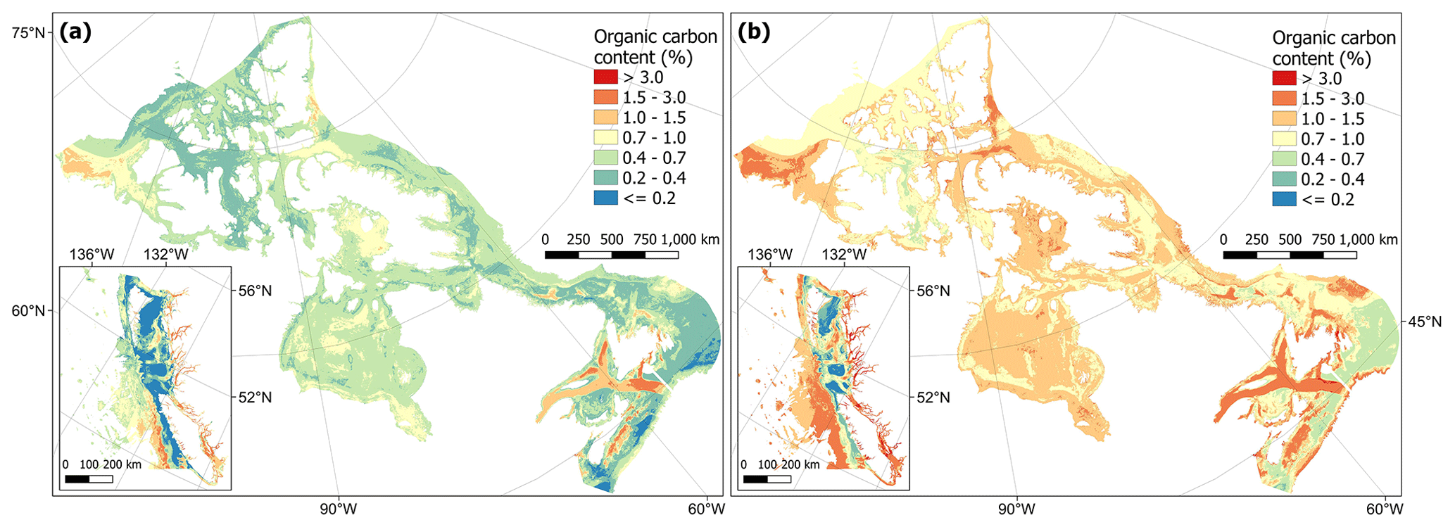
Figure E2Estimated lower (a) and upper (b) bounds of the 95 % confidence interval for predictions of carbon content (%) in sub-tidal marine sediments across the Canadian continental margin. The continuous variable is shown in discrete colour bands to improve visualisation of highly right-skewed data. Within each panel the main plot shows the Arctic and Atlantic regions with the Pacific region inset.
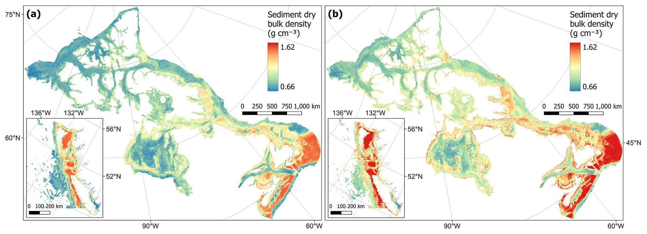
Figure E3Estimated lower (a) and upper (b) uncertainty bounds around the mean predictions of dry bulk density (g cm−3) of sub-tidal marine sediments across the Canadian continental margin. Within each panel the main plot shows the Arctic and Atlantic regions with the Pacific region inset.
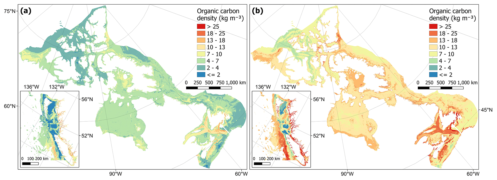
Figure E4Estimated lower (a) and upper (b) uncertainty bounds around the mean predictions of organic carbon density (kg m−3) in sub-tidal marine sediments across the Canadian continental margin. The continuous variable is shown in discrete colour bands to improve the visualisation of highly right-skewed data. Within each panel the main plot shows the Arctic and Atlantic regions with the Pacific region inset.
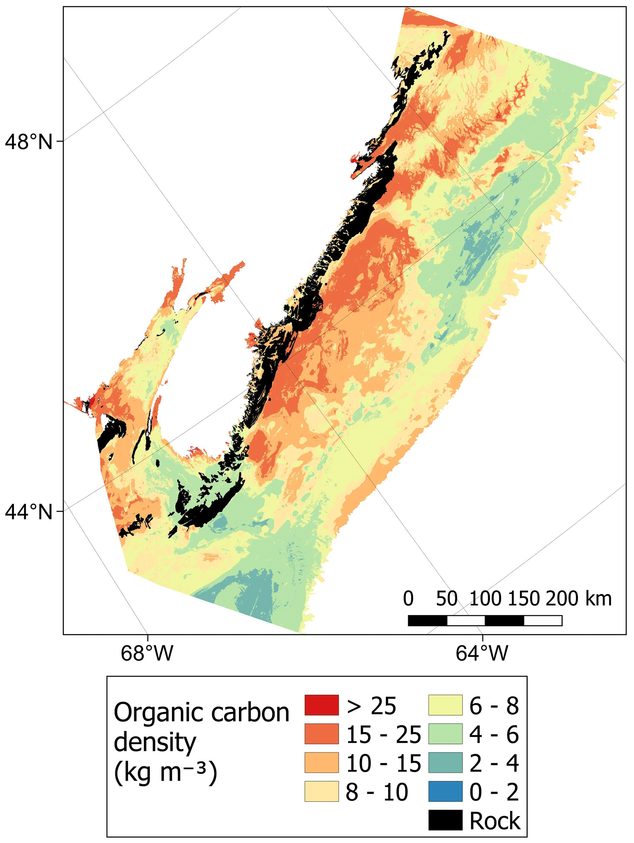
Figure F1Predicted mean values of organic carbon density within the Scotian Shelf overlain by the estimated distribution of rock substrates. Data on the estimated distribution of rock on the seafloor across the Scotian Shelf bioregion are taken from Philibert et al. (2022).
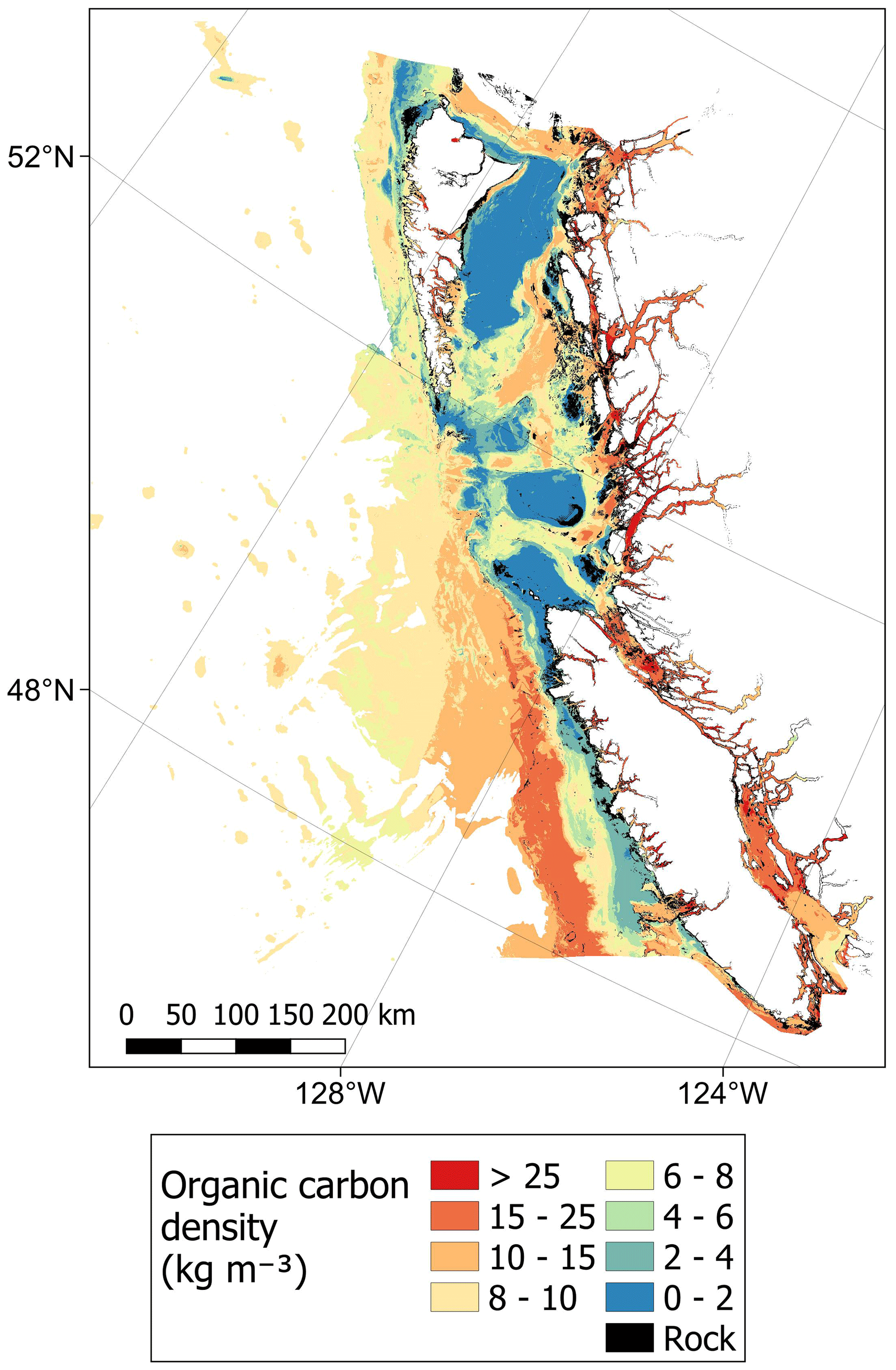
Figure F2Predicted mean values of organic carbon density within the British Columbian EEZ overlain by the estimated distribution of rock substrates. Data on the estimated distribution of rock on the seafloor across the British Columbian continental margin are taken from Gregr et al. (2021).
The supplement related to this article is available online at: https://doi.org/10.5194/essd-16-2165-2024-supplement.
JKB and SDF secured funding and led the management of this project. GE, SDF and JKB conceptualised this study. GE, DH, AP, CP and PGM collated the data. GE developed the model code and performed the investigations with input from SDF and JKB throughout. GE prepared the manuscript with contributions from all the co-authors.
The contact author has declared that none of the authors has any competing interests.
Publisher's note: Copernicus Publications remains neutral with regard to jurisdictional claims made in the text, published maps, institutional affiliations, or any other geographical representation in this paper. While Copernicus Publications makes every effort to include appropriate place names, the final responsibility lies with the authors.
We greatly appreciate advice given at various stages of the processes by Cooper Stacey, Markus Diesing, Sophia Johannessen, Ashley Park, Nadja Steiner, Diane Lavoie, Amber Holdsworth, Michael Li, Kate Jarret, Javier Murillo-Perez, Ellen Kenchington, Emily Rubidge and others at the Department for Fisheries and Oceans as well as Natural Resources Canada. We would also like to thank Randy Enkin, Sarah Paradis and Genevieve Philibert for sharing data for this work, and we are grateful for the constructive and insightful comments from the two referees as well as Jennifer McHenry, Matt Csordas and Brian Timmer for their ideas on troubleshooting during the project. This research was enabled in part by support provided by BC and Prairies Digital Research Infrastructure and the Digital Research Alliance of Canada.
This work was funded by Natural Sciences and Engineering Research Council (NSERC) Alliance partnership grant no. ALLRP571068 – 21 to Julia K. Baum and is publication no. 001 of Blue Carbon Canada. Graham Epstein is also supported by a Mitacs-Accelerate Fellowship jointly funded by Oceans North. Paul G. Myers was supported financially and logistically by grants from the NSERC, including a Discovery Grant (rgpin 227438-09), Climate Change and Atmospheric Research grants (VITALS – RGPCC433898 – and the Canadian Arctic Geotraces programme – RGPCC 433848) and the Marine Environmental Observation, Prediction and Response Network (MEOPAR) Prediction Core.
This paper was edited by Birgit Heim and reviewed by Taylor Lee and Benjamin Misiuk.
Amoroso, R. O., Pitcher, C. R., Rijnsdorp, A. D., McConnaughey, R. A., Parma, A. M., Suuronen, P., Eigaard, O. R., Bastardie, F., Hintzen, N. T., Althaus, F., Baird, S. J., Black, J., Buhl-Mortensen, L., Campbell, A. B., Catarino, R., Collie, J., Cowan, J. H., Jr., Durholtz, D., Engstrom, N., Fairweather, T. P., Fock, H. O., Ford, R., Galvez, P. A., Gerritsen, H., Gongora, M. E., Gonzalez, J. A., Hiddink, J. G., Hughes, K. M., Intelmann, S. S., Jenkins, C., Jonsson, P., Kainge, P., Kangas, M., Kathena, J. N., Kavadas, S., Leslie, R. W., Lewis, S. G., Lundy, M., Makin, D., Martin, J., Mazor, T., Gonzalez-Mirelis, G., Newman, S. J., Papadopoulou, N., Posen, P. E., Rochester, W., Russo, T., Sala, A., Semmens, J. M., Silva, C., Tsolos, A., Vanelslander, B., Wakefield, C. B., Wood, B. A., Hilborn, R., Kaiser, M. J., and Jennings, S.: Bottom trawl fishing footprints on the world's continental shelves, P. Natl. Acad. Sci. USA, 115, E10275–E10282, https://doi.org/10.1073/pnas.1802379115, 2018.
Ani, C. J. and Robson, B.: Responses of marine ecosystems to climate change impacts and their treatment in biogeochemical ecosystem models, Mar. Pollut. Bull., 166, 112223, https://doi.org/10.1016/j.marpolbul.2021.112223, 2021.
Arndt, S., Jørgensen, B. B., LaRowe, D. E., Middelburg, J. J., Pancost, R. D., and Regnier, P.: Quantifying the degradation of organic matter in marine sediments: A review and synthesis, Earth-Sci. Rev., 123, 53–86, https://doi.org/10.1016/j.earscirev.2013.02.008, 2013.
Assis, J., Tyberghein, L., Bosch, S., Verbruggen, H., Serrão, E. A., and De Clerck, O.: Bio-ORACLE v2.0: Extending marine data layers for bioclimatic modelling, Global Ecol. Biogeogr., 27, 277–284, https://doi.org/10.1111/geb.12693, 2018.
Atwood, T. B., Witt, A., Mayorga, J., Hammill, E., and Sala, E.: Global Patterns in Marine Sediment Carbon Stocks, Front. Mar. Sci., 7, 165, https://doi.org/10.3389/fmars.2020.00165, 2020.
Avelar, S., van der Voort, T. S., and Eglinton, T. I.: Relevance of carbon stocks of marine sediments for national greenhouse gas inventories of maritime nations, Carbon Balance and Management, 12, 10, https://doi.org/10.1186/s13021-017-0077-x, 2017.
Bauer, J. E., Cai, W.-J., Raymond, P. A., Bianchi, T. S., Hopkinson, C. S., and Regnier, P. A. G.: The changing carbon cycle of the coastal ocean, Nature, 504, 61–70, https://doi.org/10.1038/nature12857, 2013.
Berner, R. A.: Burial of organic carbon and pyrite sulfur in the modern ocean; its geochemical and environmental significance, Am. J. Sci., 282, 451–473, https://doi.org/10.2475/ajs.282.4.451, 1982.
Burdige, D. J.: Preservation of Organic Matter in Marine Sediments: Controls, Mechanisms, and an Imbalance in Sediment Organic Carbon Budgets?, Chem. Rev., 107, 467–485, https://doi.org/10.1021/cr050347q, 2007.
Cavan, E. L. and Hill, S. L.: Commercial fishery disturbance of the global ocean biological carbon sink, Glob. Change Biol., 28, 1212–1221, https://doi.org/10.1111/gcb.16019, 2022.
Clare, M. A., Lichtschlag, A., Paradis, S., and Barlow, N. L. M.: Assessing the impact of the global subsea telecommunications network on sedimentary organic carbon stocks, Nat. Commun., 14, 2080, https://doi.org/10.1038/s41467-023-37854-6, 2023.
Copernicus: Arctic Ocean Wave Hindcast – ARCTIC_MULTIYEAR_WAV_002_013 – Norwegian Meteorological Institute, Copernicus Marine Data Store [data set], https://doi.org/10.48670/moi-00008, 2022a.
Copernicus: Global Ocean Colour (GlobColour) – ACRI – OCEANCOLOUR_GLO_BGC_L3_MY_009_103 – Bio-Geo-Chemical, L3 (daily) from Satellite Observations (1997–ongoing), Copernicus Marine Data Store [data set], https://doi.org/10.48670/moi-00280, 2022b.
Copernicus: Global Ocean Waves Reanalysis – WAVERYS – GLOBAL_MULTIYEAR_WAV_001_032 – Mercator Océan International, Copernicus Marine Data Store [data set], https://doi.org/10.48670/moi-00022, 2022c.
DFO: Federal Marine Bioregions, Fisheries and Oceans Canada, Open Canada [data set], Record ID: 23eb8b56-dac8-4efc-be7c-b8fa11ba62e9, 2022.
Diesing, M., Kroger, S., Parker, R., Jenkins, C., Mason, C., and Weston, K.: Predicting the standing stock of organic carbon in surface sediments of the North-West European continental shelf, Biogeochemistry, 135, 183–200, https://doi.org/10.1007/s10533-017-0310-4, 2017.
Diesing, M., Thorsnes, T., and Bjarnadóttir, L. R.: Organic carbon densities and accumulation rates in surface sediments of the North Sea and Skagerrak, Biogeosciences, 18, 2139–2160, https://doi.org/10.5194/bg-18-2139-2021, 2021.
Diesing, M., Paradis, S., Jensen, H., Thorsnes, T., Bjarnadóttir, L. R., and Knies, J.: Organic Carbon Stocks and Accumulation Rates in Surface Sediments of the Norwegian Continental Margin, ESS Open Archive [preprint], https://doi.org/10.22541/essoar.170067250.09972865/v1, 2023.
Duarte, C. M., Middelburg, J. J., and Caraco, N.: Major role of marine vegetation on the oceanic carbon cycle, Biogeosciences, 2, 1–8, https://doi.org/10.5194/bg-2-1-2005, 2005.
Enkin, J. R.: Sediment Grain Size Distribution Measurements, from Canadian Pacific Seafloor Samples, Collected from 1951 to 2017, NRCan Open S&T Repository (OSTR) [data set], in press, 2024.
Epstein, G. and Roberts, C. M.: Identifying priority areas to manage mobile bottom fishing on seabed carbon in the UK, PLOS Climate, 1, e0000059, https://doi.org/10.1371/journal.pclm.0000059, 2022.
Epstein, G. and Roberts, C. M.: Does biodiversity-focused protection of the seabed deliver carbon benefits? A U.K. case study, Conserv. Lett., 16, e12929, https://doi.org/10.1111/conl.12929, 2023.
Epstein, G., Middelburg, J. J., Hawkins, J. P., Norris, C. R., and Roberts, C. M.: The impact of mobile demersal fishing on carbon storage in seabed sediments, Glob. Change Biol., 28, 2875–2894, https://doi.org/10.1111/gcb.16105, 2022.
Epstein, G., Fuller, S. D., Hingmire, D., Myers, P., Peña, A., Pennelly, C., and Baum, J. K.: Predictive maps and related data on organic carbon stocks in surficial sediments of the Canadian continental margin, Borealis V1 [data set], https://doi.org/10.5683/SP3/ICHVVA, 2024.
Evans, J. S. and Murphy, M. A.: spatialEco, R package version 1.3-6, CRAN [code], https://github.com/jeffreyevans/spatialEco (last access: 24 November 2022), 2021.
Flanders Marine Institute: Boundies of Canda EEZ – mrgid 8493, Maritime Boundaries Geodatabase: Maritime Boundaries and Exclusive Economic Zones (200NM), version 11, https://doi.org/10.14284/386, 2019.
GEBCO: GEBCO Compilation Group – GEBCO_2022 Grid, The General Bathymetric Chart of the Oceans, https://doi.org/10.5285/e0f0bb80-ab44-2739-e053-6c86abc0289c, 2022.
Gräler, B., Pebesma, E., and Heuvelink, G.: Spatio-Temporal Interpolation using gstat, R J., 8, 204–218, https://doi.org/10.32614/RJ-2016-014, 2016.
Graw, J. H., Wood, W. T., and Phrampus, B. J.: Predicting Global Marine Sediment Density Using the Random Forest Regressor Machine Learning Algorithm, J. Geophys. Res.-Sol. Ea., 126, e2020JB020135, https://doi.org/10.1029/2020JB020135, 2021.
Gregr, E. J., Haggarty, D. R., Davies, S. C., Fields, C., and Lessard, J.: Comprehensive marine substrate classification applied to Canada's Pacific shelf, PLOS ONE, 16, 1–28, https://doi.org/10.1371/journal.pone.0259156, 2021.
Gudmundsson, L., Bremnes, J. B., Haugen, J. E., and Engen-Skaugen, T.: Technical Note: Downscaling RCM precipitation to the station scale using statistical transformations – a comparison of methods, Hydrol. Earth Syst. Sci., 16, 3383–3390, https://doi.org/10.5194/hess-16-3383-2012, 2012.
Halpern, B. S., Frazier, M., Afflerbach, J., Lowndes, J. S., Micheli, F., O'Hara, C., Scarborough, C., and Selkoe, K. A.: Recent pace of change in human impact on the world's ocean, Sci. Rep., 9, 11609, https://doi.org/10.1038/s41598-019-47201-9, 2019.
Hiddink, J. G., van de Velde, S. J., McConnaughey, R. A., De Borger, E., Tiano, J., Kaiser, M. J., Sweetman, A. K., and Sciberras, M.: Quantifying the carbon benefits of ending bottom trawling, Nature, 617, E1–E2, https://doi.org/10.1038/s41586-023-06014-7, 2023.
Hijmans, R. J.: terra: Spatial Data Analysis, R package version 1.5-21, CRAN [code], https://CRAN.R-project.org/package=terra (last access: 24 November 2022), 2022.
Hilborn, R. and Kaiser, M. J.: A path forward for analysing the impacts of marine protected areas, Nature, 607, E1–E2, https://doi.org/10.1038/s41586-022-04775-1, 2022.
Hoegh-Guldberg, O., Lovelock, C., Caldeira, K., Howard, J., Chopin, T., and Gaines, S.: The ocean as a solution to climate change: five opportunities for action, World Resources Institute, Washington, DC, http://www.oceanpanel.org/climate (last access: 4 July 2023), 2019.
Hu, X., Myers, P. G., and Lu, Y.: Pacific Water Pathway in the Arctic Ocean and Beaufort Gyre in Two Simulations With Different Horizontal Resolutions, J. Geophys. Res.-Oceans, 124, 6414–6432, https://doi.org/10.1029/2019JC015111, 2019.
Hülse, D., Arndt, S., Wilson, J. D., Munhoven, G., and Ridgwell, A.: Understanding the causes and consequences of past marine carbon cycling variability through models, Earth-Sci. Rev., 171, 349–382, https://doi.org/10.1016/j.earscirev.2017.06.004, 2017.
Ilich, A. R., Misiuk, B., Lecours, V., and Lecours, S. A.: MultiscaleDTM, Zenodo [code], https://doi.org/10.5281/zenodo.5548338, 2021.
IPCC: 2019 Refinement to the 2006 IPCC Guidelines for National Greenhouse Gas Inventories, edited by: Calvo Buendia, E., Tanabe, K., Kranjc, A., Baasansuren, J., Fukuda, M., Ngarize, S., Osako, A., Pyrozhenko, Y., Shermanau, P., and Federici, S., IPCC, Switzerland, 2019.
Jakobsson, M., Mayer, L. A., Bringensparr, C., Castro, C. F., Mohammad, R., Johnson, P., Ketter, T., Accettella, D., Amblas, D., An, L., Arndt, J. E., Canals, M., Casamor, J. L., Chauché, N., Coakley, B., Danielson, S., Demarte, M., Dickson, M.-L., Dorschel, B., Dowdeswell, J. A., Dreutter, S., Fremand, A. C., Gallant, D., Hall, J. K., Hehemann, L., Hodnesdal, H., Hong, J., Ivaldi, R., Kane, E., Klaucke, I., Krawczyk, D. W., Kristoffersen, Y., Kuipers, B. R., Millan, R., Masetti, G., Morlighem, M., Noormets, R., Prescott, M. M., Rebesco, M., Rignot, E., Semiletov, I., Tate, A. J., Travaglini, P., Velicogna, I., Weatherall, P., Weinrebe, W., Willis, J. K., Wood, M., Zarayskaya, Y., Zhang, T., Zimmermann, M., and Zinglersen, K. B.: The International Bathymetric Chart of the Arctic Ocean Version 4.0, Sci. Data, 7, 176, https://doi.org/10.1038/s41597-020-0520-9, 2020.
Jenkins, C. J.: Summary of the onCALCULATION methods used in dbSEABED, in: usSEABED: Gulf of Mexico and Caribbean (Puerto Rico and U.S. Virgin Islands) Offshore Surficial Sediment Data Release: U.S, edited by: Buczkowski, B. J., Reid, J. A., Jenkins, C. J., Reid, J. M., Williams, S. J., and Flocks, J. G., United States Geological Survey, Series 146, version 1.0, http://pubs.usgs.gov/ds/2006/146/ (last access: 24 November 2022), 2005.
Keil, R.: Anthropogenic Forcing of Carbonate and Organic Carbon Preservation in Marine Sediments, Annu. Rev. Mar. Sci., 9, 151–172, https://doi.org/10.1146/annurev-marine-010816-060724, 2017.
Kuhn, M.: Building Predictive Models in R Using the caret Package, J. Stat. Softw., 28, 1–26, https://doi.org/10.18637/jss.v028.i05, 2008.
Kuhn, M. and Silge, J.: Tidy Modeling with R, O'Reilly Media, Inc, ISBN 9781492096481, 2023.
Kuhn, M. and Wickham, H.: Tidymodels: a collection of packages for modeling and machine learning using tidyverse principles, CRAN [code], https://cran.r-project.org/package=tidymodels (last access: 24 November 2022), 2020.
Kuzyk, Z. Z. A., Gobeil, C., Goñi, M. A., and Macdonald, R. W.: Early diagenesis and trace element accumulation in North American Arctic margin sediments, Geochim. Cosmochim. Ac., 203, 175–200, https://doi.org/10.1016/j.gca.2016.12.015, 2017.
LaRowe, D. E., Arndt, S., Bradley, J. A., Burwicz, E., Dale, A. W., and Amend, J. P.: Organic carbon and microbial activity in marine sediments on a global scale throughout the Quaternary, Geochim. Cosmochim. Ac., 286, 227–247, https://doi.org/10.1016/j.gca.2020.07.017, 2020a.
LaRowe, D. E., Arndt, S., Bradley, J. A., Estes, E. R., Hoarfrost, A., Lang, S. Q., Lloyd, K. G., Mahmoudi, N., Orsi, W. D., Shah Walter, S. R., Steen, A. D., and Zhao, R.: The fate of organic carbon in marine sediments – New insights from recent data and analysis, Earth-Sci. Rev., 204, https://doi.org/10.1016/j.earscirev.2020.103146, 2020b.
Lee, T. R., Wood, W. T., and Phrampus, B. J.: A Machine Learning (kNN) Approach to Predicting Global Seafloor Total Organic Carbon, Global Biogeochem. Cy., 33, 37–46, https://doi.org/10.1029/2018gb005992, 2019.
Legge, O., Johnson, M., Hicks, N., Jickells, T., Diesing, M., Aldridge, J., Andrews, J., Artioli, Y., Bakker, D. C. E., Burrows, M. T., Carr, N., Cripps, G., Felgate, S. L., Fernand, L., Greenwood, N., Hartman, S., Kröger, S., Lessin, G., Mahaffey, C., Mayor, D. J., Parker, R., Queirós, A. M., Shutler, J. D., Silva, T., Stahl, H., Tinker, J., Underwood, G. J. C., Van Der Molen, J., Wakelin, S., Weston, K., and Williamson, P.: Carbon on the Northwest European Shelf: Contemporary Budget and Future Influences, Front. Mar. Sci., 7, 143, https://doi.org/10.3389/fmars.2020.00143, 2020.
Ludwig, M., Moreno-Martinez, A., Hölzel, N., Pebesma, E., and Meyer, H.: Assessing and improving the transferability of current global spatial prediction models, Global Ecol. Biogeogr., 32, 356–368, https://doi.org/10.1111/geb.13635, 2023.
Luisetti, T., Turner, R. K., Andrews, J. E., Jickells, T. D., Kröger, S., Diesing, M., Paltriguera, L., Johnson, M. T., Parker, E. R., Bakker, D. C. E., and Weston, K.: Quantifying and valuing carbon flows and stores in coastal and shelf ecosystems in the UK, Ecosystem Services, 35, 67–76, https://doi.org/10.1016/j.ecoser.2018.10.013, 2019.
Luisetti, T., Ferrini, S., Grilli, G., Jickells, T. D., Kennedy, H., Kröger, S., Lorenzoni, I., Milligan, B., van der Molen, J., Parker, R., Pryce, T., Turner, R. K., and Tyllianakis, E.: Climate action requires new accounting guidance and governance frameworks to manage carbon in shelf seas, Nat. Commun., 11, 4599, https://doi.org/10.1038/s41467-020-18242-w, 2020.
Macreadie, P. I., Costa, M. D. P., Atwood, T. B., Friess, D. A., Kelleway, J. J., Kennedy, H., Lovelock, C. E., Serrano, O., and Duarte, C. M.: Blue carbon as a natural climate solution, Nat. Rev. Earth Environ., 2, 826–839, https://doi.org/10.1038/s43017-021-00224-1, 2021.
Madec, G., Delecluse, P., Imbard, M., and Lévy, C.: OPA 8.1Ocean General Circulation Model, Technical Report of LODYC/IPSL, Note 11, https://www.nemo-ocean.eu/wp-content/uploads/Doc_OPA8.1.pdf (last access: 2 Feburary 2023), 1998.
Mahoney, M. J., Johnson, L. K., Silge, J., Frick, H., Kuhn, M., and Beier, C. M.: Assessing the performance of spatial cross-validation approaches for models of spatially structured data, arXiv [preprint], https://doi.org/10.48550/arXiv.2303.07334, 2023.
Martens, J., Romankevich, E., Semiletov, I., Wild, B., van Dongen, B., Vonk, J., Tesi, T., Shakhova, N., Dudarev, O. V., Kosmach, D., Vetrov, A., Lobkovsky, L., Belyaev, N., Macdonald, R. W., Pieńkowski, A. J., Eglinton, T. I., Haghipour, N., Dahle, S., Carroll, M. L., Åström, E. K. L., Grebmeier, J. M., Cooper, L. W., Possnert, G., and Gustafsson, Ö.: CASCADE – The Circum-Arctic Sediment CArbon DatabasE, Earth Syst. Sci. Data, 13, 2561–2572, https://doi.org/10.5194/essd-13-2561-2021, 2021.
Martin, K. M., Wood, W. T., and Becker, J. J.: A global prediction of seafloor sediment porosity using machine learning, Geophys. Res. Lett., 42, 10640–10646, https://doi.org/10.1002/2015GL065279, 2015.
Masson, D. and Fine, I.: Modeling seasonal to interannual ocean variability of coastal British Columbia, J. Geophys. Res.-Oceans, 117, C10019, https://doi.org/10.1029/2012JC008151, 2012.
Maxwell, A. E. and Shobe, C. M.: Land-surface parameters for spatial predictive mapping and modeling, Earth-Sci. Rev., 226, 103944, https://doi.org/10.1016/j.earscirev.2022.103944, 2022.
Meyer, H. and Pebesma, E.: Machine learning-based global maps of ecological variables and the challenge of assessing them, Nat. Commun., 13, 2208, https://doi.org/10.1038/s41467-022-29838-9, 2022.
Meyer, H., Reudenbach, C., Wöllauer, S., and Nauss, T.: Importance of spatial predictor variable selection in machine learning applications – Moving from data reproduction to spatial prediction, Ecol. Modell., 411, 108815, https://doi.org/10.1016/j.ecolmodel.2019.108815, 2019.
Meyer, H., Milà, C., and Ludwig, M.: CAST: “caret” Applications for Spatial-Temporal Models, R package version 0.7.1, CRAN [code], https://CRAN.R-project.org/package=CAST (last access: 24 November 2022), 2023.
Microsoft Corporation and Weston, S.: doParallel: Foreach Parallel Adaptor for the “parallel” Package, R package version 1.0.17, CRAN [code], https://cran.r-project.org/web/packages/doParallel/index.html (last access: 24 November 2022), 2022.
Middelburg, J. J.: Reviews and syntheses: to the bottom of carbon processing at the seafloor, Biogeosciences, 15, 413–427, https://doi.org/10.5194/bg-15-413-2018, 2018.
Middelburg, J. J.: Marine Carbon Biogeochemistry: A Primer for Earth System Scientists, Springer, Cham, Switzerland, 118 pp., ISBN 978-3-030-10822-9, 2019.
Mitchell, P. J., Aldridge, J., and Diesing, M.: Legacy Data: How Decades of Seabed Sampling Can Produce Robust Predictions and Versatile Products, Geosciences, 9, 182, https://doi.org/10.3390/geosciences9040182, 2019.
Molnar, C., Bischl, B., and Casalicchio, G.: iml: An R package for Interpretable Machine Learning, JOSS, 3, 786, https://doi.org/10.21105/joss.00786, 2018.
Nellemann, C., Corcoran, E., Duarte, C. M., Valdés, L., De Young, C., Fonseca, L., and Grimsditch, G.: Blue Carbon: A Rapid Response Assessment, United Nations Environment Programme, GRID-Arendal, Norway, https://wedocs.unep.org/20.500.11822/7772, 2009.
NRCan: Lakes, Rivers and Glaciers in Canada – Hydrographic Features – Natural Resources Canada, Topographic Data of Canada – CanVec Series, Open Canada [data set], Record ID: 9d96e8c9-22fe-4ad2-b5e8-94a6991b744b, 2019.
NRCan: Canada west coast topo-bathymetric digital elevation model – Natural Resources Canada/Department of Fisheries and Oceans, Open Canada, Open Canada [data set], Record ID: e6e11b99-f0cc-44f7-f5eb-3b995fb1637e, 2021.
NRCan: The Expedition Database (ED), Natural Resources Canada – Grain Size Data, https://ed.marine-geo.canada.ca/index_e.php (last access: 21 November 2022), 2022.
Pace, M. C., Bailey, D. M., Donnan, D. W., Narayanaswamy, B. E., Smith, H. J., Speirs, D. C., Turrell, W. R., and Heath, M. R.: Modelling seabed sediment physical properties and organic matter content in the Firth of Clyde, Earth Syst. Sci. Data, 13, 5847–5866, https://doi.org/10.5194/essd-13-5847-2021, 2021.
PANGAEA®: Data Publisher for Earth & Environmental Science, PANGAEA [data set], https://doi.org/10.1594/PANGAEA, 2022.
Paradis, S., Nakajima, K., Van der Voort, T. S., Gies, H., Wildberger, A., Blattmann, T. M., Bröder, L., and Eglinton, T. I.: The Modern Ocean Sediment Archive and Inventory of Carbon (MOSAIC): version 2.0, Earth Syst. Sci. Data, 15, 4105–4125, https://doi.org/10.5194/essd-15-4105-2023, 2023.
Pebesma, E.: Simple Features for R: Standardized Support for Spatial Vector Data, R J., 10, 439–446, https://doi.org/10.32614/RJ-2018-009, 2018.
Pebesma, E. and Bivand, R.: Spatial Data Science: With applications in R. Chapman and Hall/CRC, London, https://doi.org/10.1201/9780429459016, 2023.
Pedersen, T. L.: patchwork: The Composer of Plots, R package version 1.1.2, CRAN [code], https://cran.r-project.org/package=patchwork (last access: 24 November 2022), 2022.
Peña, M. A., Fine, I., and Callendar, W.: Interannual variability in primary production and shelf-offshore transport of nutrients along the northeast Pacific Ocean margin, Deep-Sea Res. Pt. II, 169–170, 104637, https://doi.org/10.1016/j.dsr2.2019.104637, 2019.
Philibert, G., Todd, B. J., Campbell, D. C., King, E. L., Normandeau, A., Hayward, S. E., Patton, E. R., and Campbell, L.: Updated surficial geology compilation of the Scotian Shelf bioregion, offshore Nova Scotia and New Brunswick, Geological Survey of Canada – Open file, 8911, .zip file, https://doi.org/10.4095/330474, 2022.
Posit Team: RStudio: Integrated Development Environment for R, Posit Software, PBC, Boston, MA, https://posit.co/products/open-source/rstudio/ (last access: 24 November 2022), 2022.
Probst, P., Wright, M. N., and Boulesteix, A.-L.: Hyperparameters and tuning strategies for random forest, WIREs Data Mining and Knowledge Discovery, 9, e1301, https://doi.org/10.1002/widm.1301, 2019.
QGIS.org: QGIS Geographic Information System, QGIS Association, http://www.qgis.org (last access: 15 May 2023), 2021.
Raven, J.: Blue carbon: past, present and future, with emphasis on macroalgae, Biol. Lett., 14, 20180336, https://doi.org/10.1098/rsbl.2018.0336, 2018.
R Core Team: R: A language and environment for statistical computing, R Foundation for Statistical Computing, Vienna, Austria, https://www.R-project.org/ (last access: 24 November 2022), 2022.
Restreppo, G. A., Wood, W. T., Graw, J. H., and Phrampus, B. J.: A machine-learning derived model of seafloor sediment accumulation, Mar. Geol., 440, 106577, https://doi.org/10.1016/j.margeo.2021.106577, 2021.
Roy, M.-H. and Larocque, D.: Prediction intervals with random forests, Stat Methods Med. Res., 29, 205–229, https://doi.org/10.1177/0962280219829885, 2020.
Sala, E., Mayorga, J., Bradley, D., Cabral, R. B., Atwood, T. B., Auber, A., Cheung, W., Costello, C., Ferretti, F., Friedlander, A. M., Gaines, S. D., Garilao, C., Goodell, W., Halpern, B. S., Hinson, A., Kaschner, K., Kesner-Reyes, K., Leprieur, F., McGowan, J., Morgan, L. E., Mouillot, D., Palacios-Abrantes, J., Possingham, H. P., Rechberger, K. D., Worm, B., and Lubchenco, J.: Protecting the global ocean for biodiversity, food and climate, Nature, 592, 397–402, https://doi.org/10.1038/s41586-021-03371-z, 2021.
Seiter, K., Hensen, C., Schröter, J., and Zabel, M.: Organic carbon content in surface sediments–defining regional provinces, Deep-Sea Res. Pt. I, 51, 2001–2026, https://doi.org/10.1016/j.dsr.2004.06.014, 2004.
Smeaton, C., Hunt, C. A., Turrell, W. R., and Austin, W. E. N.: Marine Sedimentary Carbon Stocks of the United Kingdom's Exclusive Economic Zone, Front. Earth Sci., 9, 50, https://doi.org/10.3389/feart.2021.593324, 2021.
Snelgrove, P. V. R., Soetaert, K., Solan, M., Thrush, S., Wei, C. L., Danovaro, R., Fulweiler, R. W., Kitazato, H., Ingole, B., Norkko, A., Parkes, R. J., and Volkenborn, N.: Global Carbon Cycling on a Heterogeneous Seafloor, Trends Ecol. Evol., 33, 96–105, https://doi.org/10.1016/j.tree.2017.11.004, 2018.
Soontiens, N. and Allen, S. E.: Modelling sensitivities to mixing and advection in a sill-basin estuarine system, Ocean Model., 112, 17–32, https://doi.org/10.1016/j.ocemod.2017.02.008, 2017.
Soontiens, N., Allen, S. E., Latornell, D., Le Souëf, K., Machuca, I., Paquin, J.-P., Lu, Y., Thompson, K., and Korabel, V.: Storm Surges in the Strait of Georgia Simulated with a Regional Model, Atmos.-Ocean, 54, 1–21, https://doi.org/10.1080/07055900.2015.1108899, 2016.
Sothe, C., Gonsamo, A., Arabian, J., Kurz, W. A., Finkelstein, S. A., and Snider, J.: Large Soil Carbon Storage in Terrestrial Ecosystems of Canada, Global Biogeochem. Cy., 36, e2021GB007213, https://doi.org/10.1029/2021GB007213, 2022.
Soulsby, R. L.: Simplified calculation of wave orbital velocities, Report TR 155 – HR Wallingford, 1, http://eprints.hrwallingford.com/id/eprint/588 (last access: 10 January 2023), 2006.
Stephens, D. and Diesing, M.: Towards Quantitative Spatial Models of Seabed Sediment Composition, PLOS ONE, 10, e0142502, https://doi.org/10.1371/journal.pone.0142502, 2015.
Sumner, M.: tidync: A Tidy Approach to “NetCDF” Data Exploration and Extraction, R package version 0.3.0, CRAN [code], https://cran.r-project.org/web/packages/tidync/index.html (last access: 24 November 2022), 2022.
Turner, J. T.: Zooplankton fecal pellets, marine snow, phytodetritus and the ocean's biological pump, Prog. Oceanogr., 130, 205–248, https://doi.org/10.1016/j.pocean.2014.08.005, 2015.
Van Rossum, G. and Drake, F. L.: Python 3 Reference Manual, CreateSpace, Scotts Valley, CA, ISBN:978-1-4414-1269-0 2009.
VERRA: Methods for Monitoring of Carbon Stock Changes and Greenhouse Gas Emissions and Removals in Tidal Wetland Restoration and Conservation Project Activities (M-TW), VCS Module VMD0051, Sectoiral Scope 14, 1, https://verra.org/methodologies/methods-for-monitoring-of-carbon-stock-changes-and-greenhouse-gas-emissions-and-removals-in-tidal-wetland-restoration-and-conservation-project-activities-m-tw-v1-0/ (last access: 18 March 2023), 2020.
Wager, S., Hastie, T., and Efron, B.: Confidence Intervals for Random Forests: The Jackknife and the Infinitesimal Jackknife, J. Mach. Learn. Res., 15, 1625–1651, 2014.
Wickham, H., François, R., Henry, L., Müller, K., and Vaughan, D.: Welcome to the {tidyverse}, J. Open Source Softw., 4, 1686, https://doi.org/10.21105/joss.01686, 2019.
Wilson, R. J., Speirs, D. C., Sabatino, A., and Heath, M. R.: A synthetic map of the north-west European Shelf sedimentary environment for applications in marine science, Earth Syst. Sci. Data, 10, 109–130, https://doi.org/10.5194/essd-10-109-2018, 2018.
Wood, S. N., Pya, N., and Säfken, B.: Smoothing Parameter and Model Selection for General Smooth Models, J. Am. Stat. Assoc., 111, 1548–1563, https://doi.org/10.1080/01621459.2016.1180986, 2016.
Wright, M. N. and Ziegler, A.: {ranger}: A Fast Implementation of Random Forests for High Dimensional Data in {C} and {R}, J. Stat. Softw., 77, 1–17, 2017.
Wright, M. N., Ziegler, A., and König, I. R.: Do little interactions get lost in dark random forests?, BMC Bioinformatics, 17, 1–10, 2016.
Zhang, X., Chen, S., Xue, J., Wang, N., Xiao, Y., Chen, Q., Hong, Y., Zhou, Y., Teng, H., Hu, B., Zhuo, Z., Ji, W., Huang, Y., Gou, Y., Richer-de-Forges, A. C., Arrouays, D., and Shi, Z.: Improving model parsimony and accuracy by modified greedy feature selection in digital soil mapping, Geoderma, 432, 116383, https://doi.org/10.1016/j.geoderma.2023.116383, 2023.
- Abstract
- Introduction
- Methods
- Results
- Code and data availability
- Discussion
- Appendix A: Supplementary methods
- Appendix B: Distribution of response data
- Appendix C: Organic carbon sediment depth modelling results
- Appendix D: Results from random forest cross-validation structure selection
- Appendix E: Cell-specific uncertainty bounds for predictive sediment maps
- Appendix F: Bedrock distribution case studies
- Author contributions
- Competing interests
- Disclaimer
- Acknowledgements
- Financial support
- Review statement
- References
- Supplement