the Creative Commons Attribution 4.0 License.
the Creative Commons Attribution 4.0 License.
 | 31 Oct 2023
A new global oceanic multi-model net primary productivity data product
Thomas J. Ryan-Keogh
Sandy J. Thomalla
Nicolette Chang
Tumelo Moalusi
Net primary production of the oceans contributes approximately half of the total global net primary production, and long-term observational records are required to assess any climate-driven changes. The Ocean Colour Climate Change Initiative (OC-CCI) has proven to be robust whilst also being one of the longest records of ocean colour. However, to date, only one primary production algorithm has been applied to this data product, with other algorithms typically applied to single-sensor missions. The data product presented here addresses this issue by applying five algorithms to the OC-CCI data product, which allows the user to interrogate the range of distributions across multiple models and to identify consensus or outliers for their specific region of interest. Outputs are compared to single-sensor data missions, highlighting good overall global agreement, with some small regional discrepancies. Inter-model assessments address the source of these discrepancies, highlighting the choice of the mixed-layer data product as a vital component for accurate primary production estimates. The datasets are published in the Zenodo repository at https://doi.org/10.5281/zenodo.7849935, https://doi.org/10.5281/zenodo.7858590, https://doi.org/10.5281/zenodo.7860491 and https://doi.org/10.5281/zenodo.7861158 (Ryan-Keogh et al., 2023a, b, c, d).
- Article
(21763 KB) - Full-text XML
- BibTeX
- EndNote


Phytoplankton primary production and associated spatial and temporal variability play an important role in the carbon cycle, being responsible for approximately 50 % of total global net primary production (NPP) (Lurin, 1994; Longhurst et al., 1995; Field et al., 1998; Carr et al., 2006; Buitenhuis et al., 2013). Global NPP estimates are on the order of 50 Gt C yr−1 (Longhurst et al., 1995; Field et al., 1998; Carr et al., 2006; Buitenhuis et al., 2013; Antoine et al., 1996; Silsbe et al., 2016; Johnson and Bif, 2021). When this organic carbon is sequestered to the ocean interior via the biological carbon pump (BCP), it offsets the flux of upwelled pre-industrial dissolved inorganic carbon (DIC) (Mikaloff Fletcher et al., 2007; Gruber et al., 2009), where DIC is the carbon source for phytoplankton photosynthesis. In that sense, in the contemporary period, it does not play a significant role in the ocean uptake of anthropogenic carbon dioxide (CO2). However, the magnitude of the BCP is predicted to change in response to global climate change, which will alter the ocean's ability to store carbon and therefore impact atmospheric levels of CO2 (Henson et al., 2011; Bopp et al., 2013; Boyd et al., 2015; Tagliabue et al., 2021). Such changes are of concern because alterations in the role that the BCP plays in offsetting upwelled DIC will impact the net uptake of anthropogenic CO2 (Henson et al., 2011). As such, any natural or anthropogenic perturbations to the strength and efficiency of the BCP have the potential to drive important feedbacks to global climate change and thus need to be considered for a comprehensive understanding of the trajectory of the ocean carbon sink. Recent studies have estimated that global NPP is indeed changing, with declines ranging from 0.6 % to 13 % across equatorial and temperate regions (Gregg and Rousseaux, 2019; Polovina et al., 2011; Chavez et al., 2010; Behrenfeld et al., 2006) and increases of up to 2 % at the Bermuda Atlantic Time Series and Hawaii Oceanic Time Series (Saba et al., 2010). NPP also plays an important role in supporting ecosystem function by sustaining biodiversity and the transfer of carbon, energy, and nutrients through pelagic and benthic food webs. As such, any changes to the amount of bulk carbon being produced are likely to impact the amount of carbon available for transfer to higher trophic levels via the marine food web, with implications for ecosystem health and fishery success. It is the seasonal cycle that sets much of the environmental variability in the factors that drive NPP, and it is the dominant mode of variability that couples the physical mechanisms of climate forcing to ecosystem response in production, diversity, and carbon export (Monteiro et al., 2011). As such, understanding the seasonal evolution of NPP can provide a sensitive index of climate variability through its dependence on physical processes that transport nutrients and control the exposure of phytoplankton to sunlight (Summer and Lengfeller, 2008; Henson et al., 2009). It is with this in mind that we seek to provide a data product that can be used to understand the extent to which the seasonal characteristics of NPP are being modified by environmental conditions over sufficiently long time periods. NPP has already been highlighted as a better indicator of environmental change and disturbances in comparison to chlorophyll a (Tilstone et al., 2023), with environmental disturbances (i.e, changes in nutrient inputs) being detected through changes in phytoplankton photosynthetic rates and NPP (Boalch, 1987), highlighting its suitability for ecosystem assessment of tipping points and abrupt change.
Phytoplankton NPP is strongly influenced by the physico-chemical conditions of the ocean, including light, temperature, and nutrient availability. Climate change has already begun to elicit widespread changes to these conditions; for example, increases in temperature and heat content, increased sea ice melt, and enhanced precipitation all contribute to alterations of oceanic density and the subsequent nutrient supply into the euphotic zone (IPCC, 2014; Rhein et al., 2013). Being able to understand how these climate-driven changes in the physico-chemical environment impact phytoplankton NPP is key to addressing one of the most important scientific and policy challenges of the 21st century, namely being able to predict long-term trends in the ocean-carbon–climate system. This challenge is exacerbated by the sparsity of NPP data and a lack of continuous or regular in situ measurements for long-enough periods to address multi-decadal changes associated with climate forcing (Johnson and Bif, 2021).
Satellite-based remote sensing of ocean colour is the only observational capability that can provide synoptic views of upper-ocean phytoplankton characteristics at high spatial and temporal resolutions (∼ 1 km, ∼ daily) and high temporal extents (global scales, years to decades). In many cases, these are the only systematic observations available for chronically under-sampled marine systems such as the Southern Ocean. Empirical expressions of estimating NPP are built around long-recognized dependencies between phytoplankton biomass and environmental conditions (e.g. temperature, light, and nutrients), with a succinct review available in Westberry et al. (2023). The vertically generalized production model (VGPM) (Eppley, 1972; Behrenfeld and Falkowski, 1997) is a simpler satellite NPP model that relies on the relationship between chlorophyll- and temperature-derived growth rates with no explicit spectral, temporal, or vertical resolution. The carbon-based production models (CbPMs; Behrenfeld et al., 2005; Westberry et al., 2008) rely on particulate backscattering estimates of phytoplankton carbon as a biomass indicator instead of chlorophyll. This approach allows for some of the variability in chlorophyll to be attributed to physiological adjustments to light and nutrients (e.g. photoacclimation), independent of changes in NPP. The more recent CAFE model (Silsbe et al., 2016) builds upon this approach but in addition incorporates the influence of non-algal absorption on the attenuation of the underwater light field, which, if not accounted for, has a tendency to overestimate NPP (notably in coastal waters). Recently, considerable effort has been invested by the European Space Agency to provide one of the longest records of ocean colour for detecting climate variability by merging data from SeaWIFS, MODIS, MERIS, VIIRS, Sentinel 3A OLCI, and Sentinel 3B OLCI and by correcting inter-sensor biases from the multiple ocean colour satellite sensors (Sathyendranath et al., 2019a); this is known as the Ocean Colour Climate Change Initiative (OC-CCI). This time series of 25 years (as of 2023) has already been utilized to provide estimates of trends in global NPP (Kulk et al., 2020), with results showing that trends in NPP were linked to trends in chlorophyll a and related to changes in the physico-chemical conditions of the water column from inter-annual and multi-decadal climate oscillations. However, this study only investigated one NPP algorithm as opposed to using a suite of different algorithms with varying sensitivities to specific processes, as is done for the assessments of predicted change from Earth system models in the coupled model intercomparison project (CMIP). It is worth noting, however, that previous studies have performed a series of statistical evaluations of a range of NPP models, known as the primary production algorithm round robin (Campbell, et al., 2002; Carr et al., 2006; Friedrichs et al., 2009; Saba et al., 2011; Lee et al., 2015), utilizing in situ measurements and satellite matchups to assess their relative performance, with the CAFE model most recently having the lowest bias and error in comparison to all other algorithms available at the time.
Given the importance of NPP for assessing carbon budgets, ecosystem health, and environmental change, it is becoming increasingly clear that users require easy access to appropriate data products. Unfortunately, the global NPP algorithm applied to OC-CCI by Kulk et al. (Kulk et al., 2020) is not available for download on the OC-CCI server. Although an NPP data product is available from Copernicus Marine Services, this is only applied to the temporally limited GlobColour data product and similarly is only available for a single NPP algorithm (Antoine and Morel, 1996). The most comprehensive suite of NPP algorithms is provided by the Ocean Productivity website (http://sites.science.oregonstate.edu/ocean.productivity/custom.php, last access: 1 September 2023); however, these are also only applied to single-sensor missions (SeaWIFS, MODIS, VIIRS), thus restricting time periods of interest and preventing any longer-term assessments of change. Furthermore, it is difficult for the user to ascertain exactly which ancillary data products (i.e. MLD criterion, nitracline) were used in the empirical derivations of the single-sensor NPP products available for download.
Here, we present a new ocean colour data product that incorporates five NPP algorithms applied to the 25-year merged-sensor OC-CCI time series. This multi-model data product provides a range of estimates of global NPP from 1998 to 2022 at both 8 d and monthly resolutions and at a spatial coverage of 25 km. The distributions of the models are assessed across different oceanic biomes and long-term observatory sites to highlight either consensus or outliers. The outputs of these algorithms are assessed for any biases or differences in comparison to the original outputs from single-sensor missions and for intra-algorithm differences for the multi-sensor satellite record.
A total of 25 years of ocean colour data from 1998–2022 were downloaded from the OC-CCI server (8 d, 4 km, v6.0; Sathyendranath et al., 2019a), in which the latest version, v6.0, includes an updated MERIS-4th reprocessing and Sentinel 3B OLCI, drops MODIS and VIIRS data after 2019, and uses the quasi-analytical algorithm (QAA) (Lee et al., 2002). The data variables downloaded from OC-CCI v6.0 include chlorophyll a concentration (Chl a, mg m−3), backscatter at 443 nm (bbp, m−1), the diffuse attenuation coefficient at 490 nm (Kd 490, m−1), the phytoplankton absorption coefficient at 443 nm (aph, m−1), and the detrital absorption coefficient at 443 nm (adg, m−1). As the spectral slope of bbp (η, m−1 nm−1) is not a variable provided by the OC-CCI project, it had to be calculated following Eq. (1) from Pitarch et al. (2019) using remote sensing reflectance (Rrs) at 443 and 560 nm. Daily integrated photosynthetically active radiation (PAR, ) data were downloaded from Glob-Colour (http://www.globcolour.info/, last access: 1 September 2023). Sea surface temperature (SST, ∘C) data were downloaded from the Group for High-Resolution Sea Surface Temperature (GHRSST; https://www.ghrsst.org/, last access: 1 September 2023). The Hadley EN4.2.2 gridded temperature and salinity profiles (Good et al., 2013) were converted to density (σ, kg m−3) to derive mixed-layer depth (MLD, m) using the density thresholds of 0.03 kg m−3 (de Boyer Montégut et al., 2004) and 0.125 kg m−3 (Suga et al., 2004). Additional data for MLD were retrieved from HYCOM (https://www.hycom.org/data/glba0pt08, last access: 1 September 2023) for both density criteria (downloaded from http://sites.science.oregonstate.edu/ocean.productivity/, last access: 1 September 2023).
For the primary analysis of the paper, the outputs using the Hadley Δσ10 m = 0.030 kg m−3 MLD data product were used (Ryan-Keogh et al., 2023d). The reason for this choice was concerns around the accuracy of the HYCOM MLD data product in best representing in situ conditions. A trend analysis performed on all MLD products and criteria (Fig. A1 in the Appendix) revealed distinct directional differences in the trends of Hadley versus HYCOM, with the Hadley MLD product being the only one to best represent the global MLD trends as outlined in Sallée et al. (2021). However, the outputs using Hadley Δσ10 m = 0.125 kg m−3 (Ryan-Keogh et al., 2023a), HYCOM Δσ10 m = 0.030 kg m−3 (Ryan-Keogh et al., 2023b), and HYCOM Δσ10 m = 0.125 kg m−3 (Ryan-Keogh et al., 2023c) are all available.
The nitracline depth was defined as the depth at which nitrate and nitrite were equal to 0.5 µM (Westberry et al., 2008) using the monthly climatology nitrate and nitrite profile data from the World Ocean Atlas 2018 (WOA18; (Garcia et al., 2019). The total backscattering of pure seawater (bbw, m−1) was derived as a function of SST and salinity following Zhang and Hu (2009) using monthly salinity data from WOA18 averaged for the top 20 m.
All data were regridded onto a regular grid of 25 km spatial resolution using bilinear interpolation using the xESMF Python package (Zhuang et al., 2023) at 8 d temporal resolution. The remaining gaps were filled by applying a linear interpolation scheme in sequential steps of longitude, latitude, and time (Racault et al., 2014) using a three-point window. If one of the points bordering the gap along the indicated axis was invalid, it was omitted from the calculation, whilst if two surrounding points were invalid, then the gap was not filled. Finally, the data were smoothed by applying a moving-average filter of the previous and next time steps. For more details on this method, see Salgado-Hernanz et al. (2019).
Table 1Data variables, including chlorophyll a (Chl a, mg m−3), photosynthetically active radiation (PAR, ), backscatter at 443 nm (bbp, m−1), phytoplankton absorption at 443 nm (aph, m−1), detrital absorption at 443 nm (adg, m−1), diffuse attenuation coefficient at 490 nm (Kd, m−1), the spectral slope of backscatter (η, ), the backscatter of pure water (bbw, m−1), mixed-layer depth (MLD, m), sea surface temperature (SST, ∘C), nitracline depth (m), and sea surface salinity (SSS), used in the derivation of net primary production using five models, namely the Eppley-VGPM, Behrenfeld-VGPM, Behrenfeld-CbPM, Westberry-CbPM, and Silsbe-CAFE.
NPP () was calculated using five different algorithms, namely the Eppley-VGPM model (Eppley, 1972), the Behrenfeld-VGPM model (Behrenfeld and Falkowski, 1997), the Behrenfeld-CbPM model (Behrenfeld et al., 2005), the Westberry-CbPM model (Westberry et al., 2008), and the Silsbe-CAFE model (Silsbe et al., 2016). Both Eppley-VGPM and Behrenfeld-VGPM models are chlorophyll-based production models with a temperature-dependent derivation of photosynthetic efficiencies. The Behrenfeld-CbPM and Westberry-CbPM models are based upon deriving carbon biomass from backscatter coefficients and growth rates from chlorophyll-to-carbon ratios, with the Westberry-CbPM being spectrally resolved across nine wavelengths. The Silsbe-CAFE model is an absorption-based model that is spectrally resolved across 21 wavelengths whilst also being resolved across the diel cycle from sunrise to sunset. For more details on which parameters are required for each model, please see Table 1.
For presentation purposes, the global data were separated into biomes using the classification from Fay and McKinley (2014), while long-term observatories were selected to be the Bermuda Atlantic Time Series (30.7–32.7∘ N, 59.2–61.2∘ W), the Hawaii Oceanic Time Series (21.8–23.8∘ N, 157–159∘ W), the Southern Ocean Time Series (46.0–48.0∘ S, 139–141∘ E), and the Porcupine Abyssal Plain observatory (48–50∘ N, 15.5–17.5∘ W).
As an additional comparison to the OC-CCI outputs presented here, monthly NPP data of Eppley-VGPM, Behrenfeld-VGPM, Westberry-CbPM, and Silsbe-CAFE were downloaded from the Ocean Productivity website (http://sites.science.oregonstate.edu/ocean.productivity/, last access: 1 September 2023) for SeaWIFS (1998–2007) and MODIS (2003–2019). Unfortunately, the NPP data for the Behrenfeld-CbPM are no longer available as they have been superseded by the Westberry-CbPM NPP data. Pearson's correlation coefficients (R2) were calculated between the SeaWIFS- and MODIS-derived NPP and the OC-CCI-derived NPP.
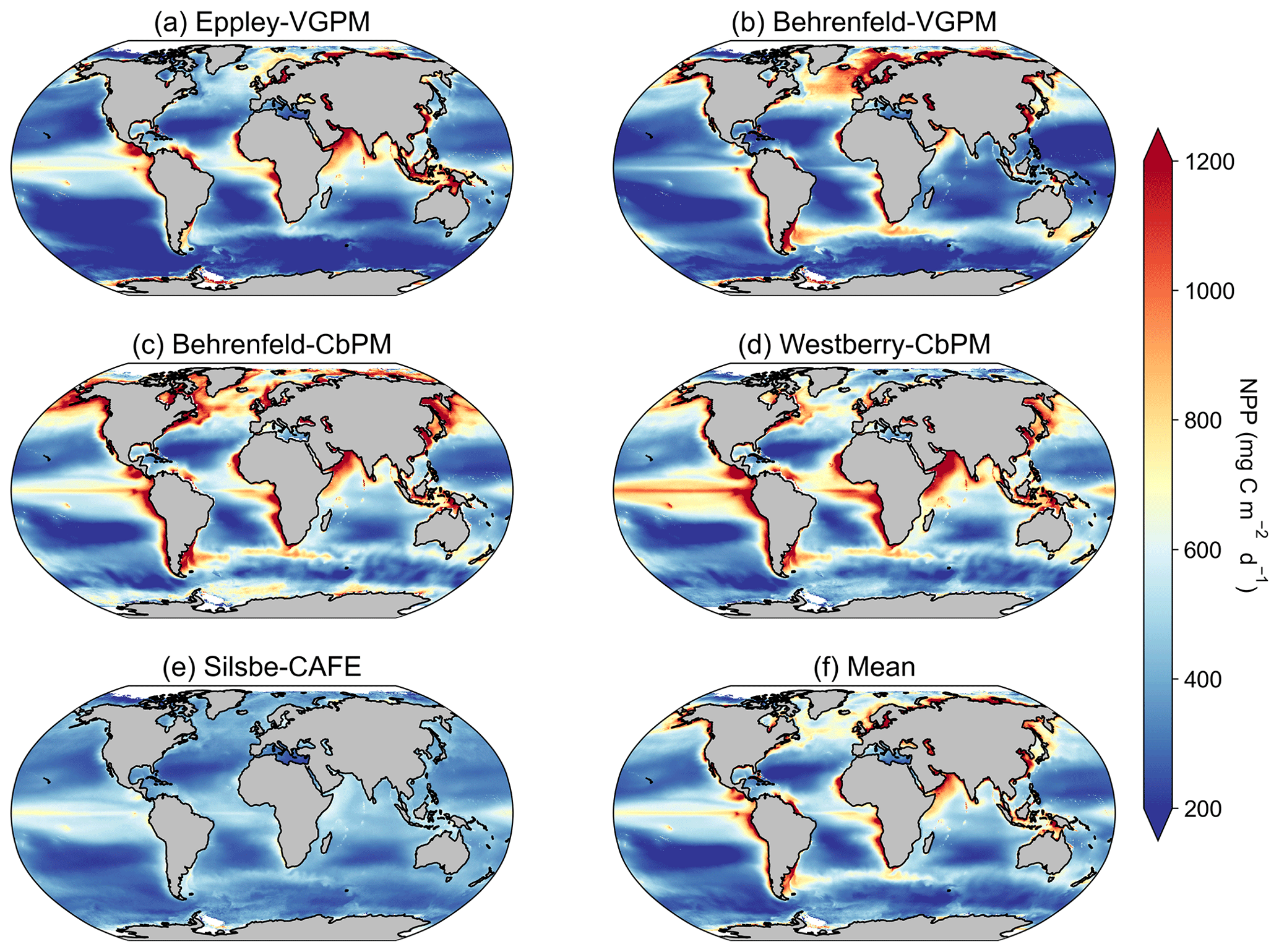
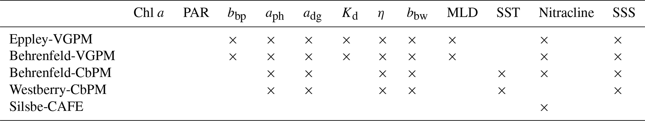
Figure 1Climatological means of net primary productivity (NPP) for the period of 1 January 1998 to 31 December 2022 for the (a) Eppley-VGPM, (b) Behrenfeld-VGPM, (c) Behrenfeld-CbPM, (d) Westberry-CbPM, and (e) Silsbe-CAFE model and (f) the mean of all models.
Figure 2The distribution of the model net primary production (NPP) values. (a) The coefficient of variation, calculated as the inter-model standard deviation normalized to the inter-model mean. (b) Probability distributions (PDFs) of the climatological mean NPP for each of the models. (c) Cumulative distributions (CDFs) of the climatological mean NPP for each of the models.
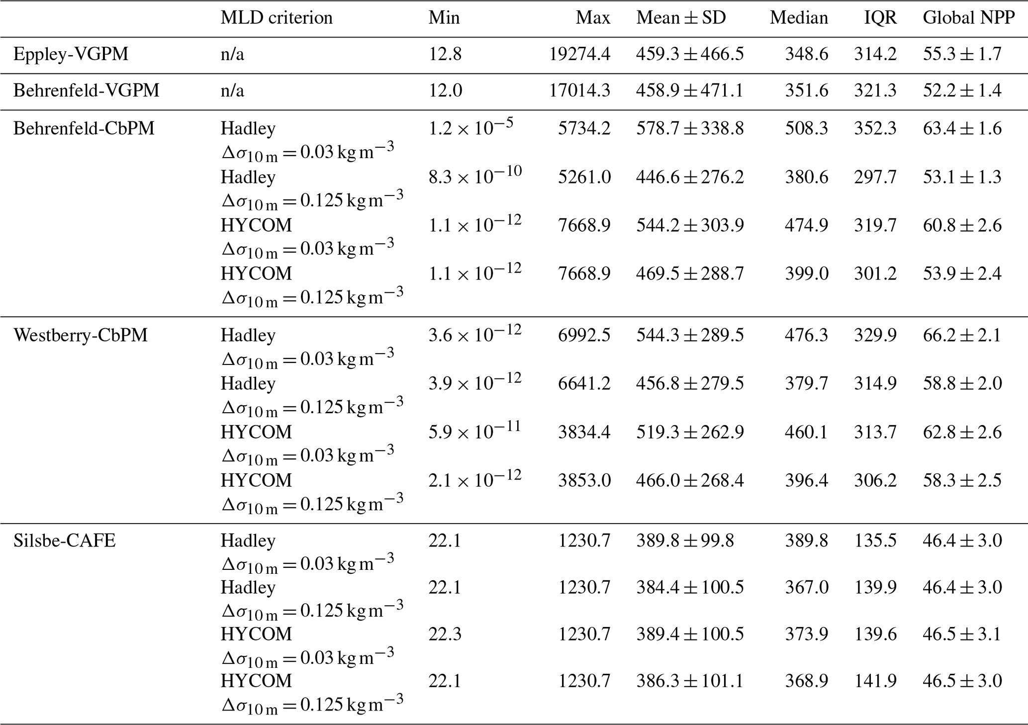
Table 2The climatological global minimum, maximum, mean ± standard deviation, median, and interquartile range (IQR: 75th–25th) for each net primary production model. Included is the sum of the global NPP () from each model (averaged for each year from 1998 to 2022, including the standard deviation), including the different MLD criteria used (where n/a means not applicable).
Comparing intra-model climatological means
The climatological means of each NPP model show a large degree of spatial heterogeneity, with higher values being associated with western boundary currents and the Equator (Fig. 1). The temperature based Eppley-VGPM and Behrenfeld-VGPM models (Fig. 1a and b) show good agreement in terms of their ranges and means (Table 2), but there are large differences, particularly in the North Atlantic and the Arabian Sea and equatorial Pacific. The carbon-based Behrenfeld-CbPM and Westberry-CbPM models (Fig. 1c and d) show very good agreement in terms of their climatological means, although discrepancies are nonetheless evident (e.g. higher NPP in the Southern Ocean and North Atlantic in the Behrenfeld-CbPM and higher NPP in the equatorial region in the Westberry-CbPM). The absorption-based Silsbe-CAFE model (Fig. 1e) has a much smaller range across the global ocean. A map of the coefficient of variation (CV = ; Fig. 2a) shows the highest values (depicting disagreement between models) in the high latitudes and in coastal regions. Unlike the comparison in Westberry et al. (2023) (which included Behrenfeld-VGPM, Westberry-CbPM, and Silsbe-CAFE applied to MODIS data from 2003 to 2019), we do not find lower CV values to be specifically associated with highly productive waters, nor do we find a similar distribution for very high CV values. The Silsbe-CAFE model has the most peaked probability distributions (PDFs) of all the models (Fig. 2b) with a narrow range, which is similar to that reported in Westberry et al. (2023). The other models show a much lower peak and broader range, with the two CbPM models centred around a lower median distribution of NPP (more similar to that of Silsbe-CAFE) than the slightly higher median NPP of the two VGPM models. When we examine the cumulative distributions (CDFs) of each model (Fig. 2c), the medians were 1 order of magnitude higher in the Eppley-VGPM (1019.5 ) and Behrenfeld-VGPM (1206.6 ) in comparison to the Behrenfeld-CbPM (298.2 ), Westberry-CbPM (531.1 ), and Silsbe-CAFE (495.5 ). Whilst the median values for both Westberry-CbPM and Silsbe-CAFE are similar to those reported in Westberry et al. (2023), the Behrenfeld-VGPM values are much higher than what was previously reported (332 ), which is not necessarily surprising when considering the fact that different SST, PAR, and Chl a products are being used in this analysis.
Investigating the difference in climatological means between each model and the ensemble model mean highlights the regional distribution of positive and negative biases relative to the ensemble model mean (Fig. A2). For example, the two VGPM models show an opposite distribution in their relative differences, with Behrenfeld-VGPM being higher in the North Atlantic, Arctic, and Antarctic Circumpolar Current (ACC) regions, while Eppley-VGPM is higher in the equatorial region. Both CbPM models show a tendency to overestimate NPP compared to other models, except in the Arctic, where the Westberry-CbPM is instead lower than the ensemble model mean. Interestingly, although the climatological mean of the Silsbe-CAFE appears to be lower than that of all other models (Fig. 1), this is not globally consistent when expressed as a difference, which instead highlights that the Silsbe-CAFE overestimates NPP relative to other models in the oligotrophic gyres and ACC region. Finally, if we compare global oceanic NPP from the models with previous IPCC estimates of 50 , all models have similar ranges (between 46.4–66.2 ) to those previously reported (32.0–70.7 ; Buitenhuis et al., 2013; Sathyendranath et al., 2019b).
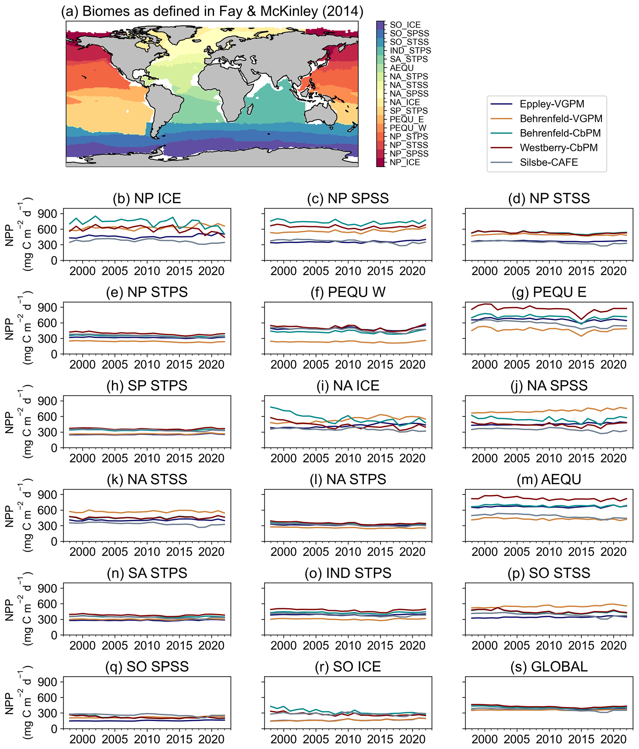
Figure 3(a) Map of the mean biomes from Fay and McKinley (2014), where white areas represent regions which do not fit into any biome classification. Annual means of net primary productivity (NPP, ) from the Eppley-VGPM, Behrenfeld-VGPM, Behrenfeld-CbPM, Westberry-CbPM, and Silsbe-CAFE models for the (b) North Pacific ice biome (NP ICE), (c) North Pacific subpolar seasonally stratified biome (NP SPSS), (d) North Pacific subtropical seasonally stratified biome (NP STSS), (e) North Pacific subtropical permanently stratified biome (NP STPS), (f) West Pacific equatorial biome (PEQU W), (g) East Pacific equatorial biome (PEQU E), (h) South Pacific subtropical permanently stratified biome (SP STPS), (i) North Atlantic ice biome (NA ICE), (j) North Atlantic subpolar seasonally stratified biome (NA SPSS), (k) North Atlantic subtropical seasonally stratified biome (NA STSS), (l) North Atlantic subtropical permanently stratified biome (NA STPS), (m) equatorial Atlantic biome (AEQU), (n) South Atlantic subtropical permanently stratified biome (SA STPS), (o) Indian subtropical permanently stratified biome (IND STPS), (p) South Ocean subtropical seasonally stratified biome (SO STSS), (q) Southern Ocean subpolar seasonally stratified biome (SO SPSS), (r) Southern Ocean ice biome (SO ICE), and (s) the global ocean.
Interrogating spatio-temporal patterns of NPP data products
Fay and McKinley (2014) classified the global ocean into 17 biomes (Fig. 3) according to distinct biological (Chl a concentrations) and physical characteristics (SST, MLD, and ice fraction). Splitting the NPP data according to these biomes allows a regional comparison of inter-model differences and similarities. The annual model means of each NPP product range from a minimum value of 212.15 ± 39.25 in the Southern Ocean subpolar seasonally stratified (SO SPSS) biomes (Fig. 3s) to a maximum value of 654.50 ± 141.18 in the East Pacific equatorial biome (PEQU E) biome (Fig. 3g). When globally averaged (Fig. 3s), the models appear to agree very well in their annual climatologies of NPP; however, when interrogated on a per-biome basis, some discrepancies emerge. For example, although there is particularly good agreement in NPP in the oligotrophic gyres (Fig. 3e, h, l, and n), large intra-model differences are particularly evident in the equatorial biomes (Fig. 3f, g, and m) and the high-latitude Atlantic and Pacific (Fig. 3b, c, i, and j). In some biomes, there is also a tendency for models to merge or diverge over time. For example, there is a large inter-model spread in the early 2000s in the North Atlantic and Southern Ocean ICE biomes (Fig. 3i and r), which narrows over time, while the opposite is apparent in the North Atlantic subpolar seasonally stratified biome (NA SPSS) biome (Fig. 3j). Also worth noting are regions where all models agree except one, for example, the comparatively lower NPP for the Behrenfeld-VGPM model in the West Pacific equatorial biome (PEQU W) (Fig. 3f).
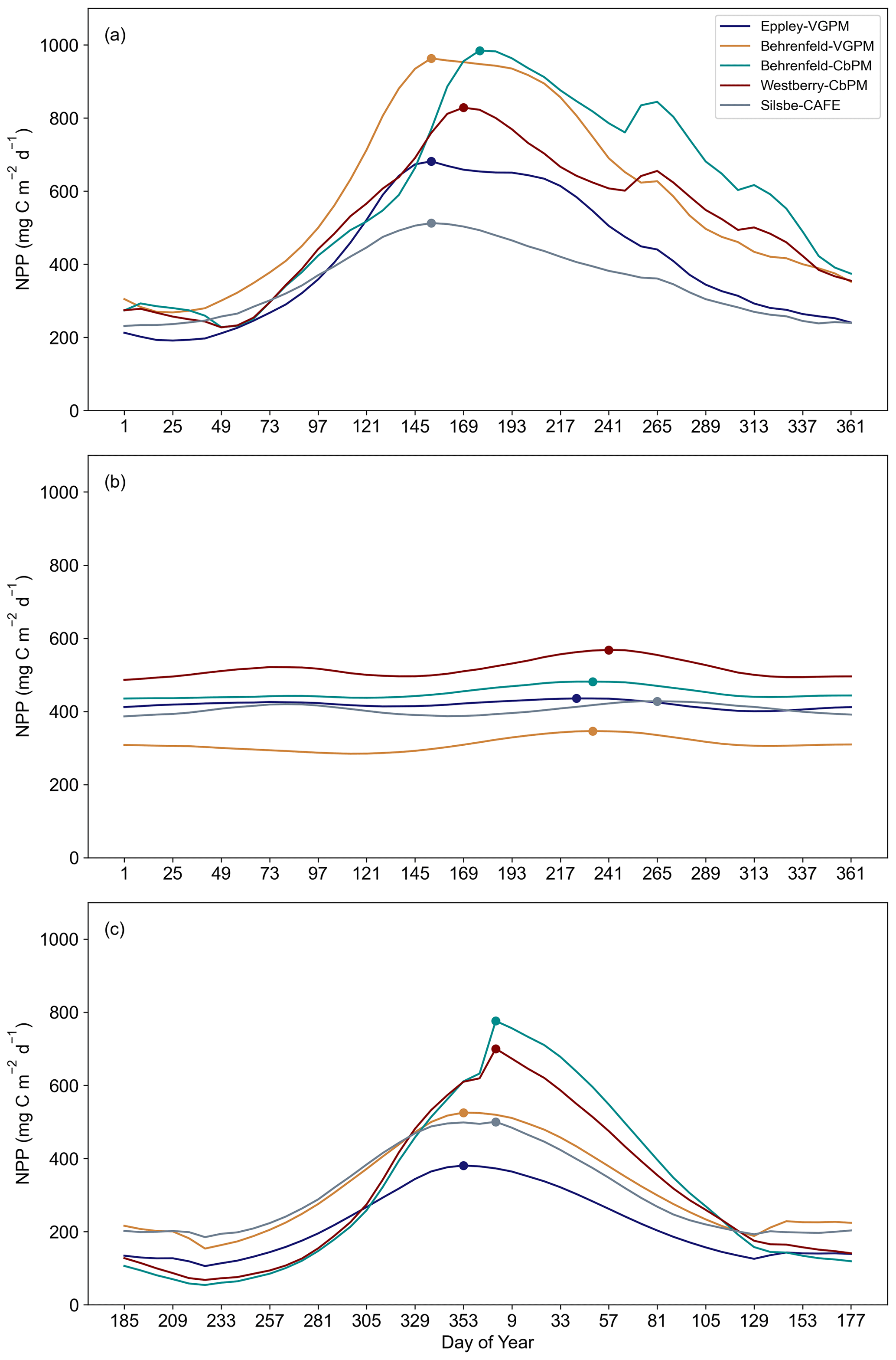
Figure 4The seasonal cycle of net primary productivity (NPP, ) from the Eppley-VGPM, Behrenfeld-VGPM, Behrenfeld-CbPM, Westberry-CbPM, and Silsbe-CAFE models for (a) the northern high-latitude regions (NA ICE, NP ICE, NA SPSS, NP SPSS, NA STSS, and NP STSS), (b) the equatorial and low-latitude regions (AEQU, PEQU E, PEQU W, IND STPS, NA STPS, SA STPS, NP STPS, and SP STPS), and (c) the southern high-latitude regions (SO ICE, SO SPSS, and SO STSS). Data are averaged across the time period 1998–2022. Please note that, for panel (c), the data have been shifted for the peak to appear in the centre of the plot. The circles represent the timing of the annual maximum.
In the next model comparison, we combine biomes into three regions, namely northern high latitude, equatorial, and southern high latitude, to examine the seasonal cycle in NPP across the five models. Here, inter-model differences become even more pronounced in terms of their minima, maxima, and phenology of the seasonal cycle (Fig. 4). In the Northern Hemisphere's biomes (Fig. 4a; North Pacific and North Atlantic ice, subpolar seasonally stratified, and subtropical seasonally stratified biomes), there is a large range of variability in maximum NPP, with the Behrenfeld-VGPM and Behrenfeld-CbPM exhibiting the highest peak values (963.08 and 984.36 , respectively) and the Silsbe-CAFE model exhibiting the lowest peak value (512.57 ). The timings of the peaks are also offset, with the earliest peak occurring in the Eppley-VGPM, Behrenfeld-VGPM, and Silsbe-CAFE models at the start of June, while the Behrenfeld-CbPM and Westberry-CbPM models put the timing of the peak a few weeks later in mid-June. The Southern Hemisphere's biomes (Fig. 4c; Southern Ocean ice, subpolar seasonally stratified, and subtropical seasonally stratified biomes) similarly express a large range in amplitude of the seasonal peak across all models, with both CbPM models exhibiting the highest values (776.17 and 700.27 , respectively), whereas the Eppley-VGPM exhibits the lowest peak value (380.82 ). The timing of the peak is similar for Behrenfeld-CbPM, Westberry-CbPM, and Silsbe-CAFE in January with the Eppley-VGPM and Behrenfeld-VGPM models placing the bloom peak earlier in December. The low-latitude and equatorial biomes (Fig. 4b; North South Pacific subtropical permanently stratified, North South Atlantic subtropical permanently stratified, Indian subtropical permanently stratified, and Atlantic and Pacific equatorial biomes) do not exhibit any clear seasonal cycle and have a lower range of variability across all the models. The range of divergence is more similar to that of the seasonal troughs of NPP in the northern and southern high-latitude regions, although rates of NPP are not as low (mean for all models for the time series = 420.69 ± 75.06 ).
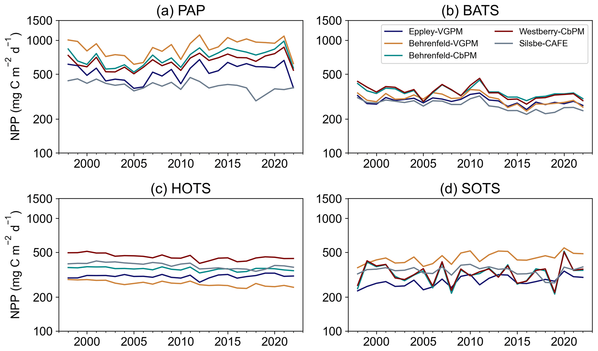
Figure 5Annual means of net primary productivity (NPP, ) from the Eppley-VGPM, Behrenfeld-VGPM, Behrenfeld-CbPM, Westberry-CbPM, and Silsbe-CAFE models for (a) the Porcupine Abyssal Plain (PAP) observatory, (b) the Bermuda Atlantic Time Series (BATS), (c) the Hawaii Oceanic Time Series (HOTS), and (d) the Southern Ocean Time Series (SOTS).
We further examined the variability between models by choosing four long-term observatory sites, namely the Porcupine Abyssal Plain observatory (PAP; Fig. 5a), the Bermuda Atlantic Time Series (BATS; Fig. 5b), the Hawaii Oceanic Time Series (HOTS; Fig. 5c), and the Southern Ocean Time Series (SOTS; Fig. 5d). The BATS site has the lowest range of NPP with the smallest inter-model differences (310.11 ± 35.37 ), while HOTS and SOTS express a similar range in NPP (352.86 ± 73.46 345.79 ± 62.22 , respectively), and the PAP site has the highest range in NPP and the greatest inter-model differences (632.00 ± 180.45 ).
Comparison with MODIS- and SeaWIFS-derived NPP
When first designed, these NPP models were originally implemented in both SeaWIFS and MODIS data products. As such, we are able to compare the new OC-CCI-derived NPP for all models presented here with the original NPP from both SeaWIFS and MODIS that is downloadable from the Ocean Productivity website (http://sites.science.oregonstate.edu/ocean.productivity/, last access: 1 September 2023). Spatial correlation maps were subsequently derived for the Eppley-VGPM, Behrenfeld-VGPM, Westberry-CbPM, and Silsbe-CAFE models using both SeaWIFS- and OC-CCI-derived NPP for the period of 1 January 1998 to 31 December 2007 (Fig. A3) and the MODIS- and OC-CCI-derived NPP for the period 1 January 2003 to 31 December 2019 (Fig. A4). Results show very good agreement for Eppley-VGPM (Figs. A3a, b and A4a, b) and Behrenfeld-VGPM (Figs. A3c, d and A4c, d) for both SeaWIFS (median R2 = 0.83 and 0.87, respectively) and MODIS (median R2 = 0.85 and 0.90, respectively), with some lower R2 values evident in the equatorial region. Correlations were generally poor for the Westberry-CbPM model for both SeaWIFS (median R2 = 0.41) and MODIS (median R2 = 0.52). Correlations against the Silsbe-CAFE model were good at higher latitudes for both SeaWIFS and MODIS but poor in the equatorial region, with the overall correlation being worse for MODIS (median R2 = 0.66) than for SeaWIFS (median R2 = 0.70). However, the NPP data products generated from SeaWIFS and MODIS for these respective time periods were derived using the HYCOM MLD data product and not Hadley (as per the OC-CCI NPP product), which may account for some of the observed variability and poor correlations. For consistency, we can instead similarly use the HYCOM MLD with a density criterion of Δσ10 m = 0.030 kg m−3 (Fig. A5) to derive the OC-CCI NPP product for comparison with SeaWIFS and MODIS products for the Westberry-CbPM and Silsbe-CAFE models (which both use MLD as input criteria, unlike the VGPM models) (Ryan-Keogh et al., 2023b). Here, we see an overall improvement in the spatial correlation maps and distribution of R2, which, for Westberry-CbPM, increased in both SeaWIFS and MODIS to R2 = 0.51 and 0.60, respectively, while for the Silsbe-CAFE model the correlation increased to R2 = 0.76 and 0.70 (for SeaWIFS and MODIS, respectively).
The reasons for discrepancies between NPP products derived from OC-CCI versus SeaWIFS and MODIS can culminate from differences in the satellite products themselves (which will not be investigated here) but also from additional sources of variability that stem primarily from differences in the criteria of input variables. For instance, the original Westberry-CbPM study used a mixed-layer definition of ΔT10 m = 0.5 ∘C, whereas the NPP products applied here use a density criteria of Δσ10 m = 0.030 kg m−3. If we instead derive NPP from an MLD that is defined with a density criteria of Δσ10 m = 0.125 kg m−3 (as per the alternative MLD criterion listed on the Ocean Productivity website, http://sites.science.oregonstate.edu/ocean.productivity/, last access: 1 September 2023) (Ryan-Keogh et al., 2023c), we see a further improvement in the spatial correlation of NPP for the Westberry-CbPM (Fig. A5a-d), for both SeaWIFS (R2 = 0.65) and MODIS time periods (R2 = 0.74), and for the Silsbe-CAFE model for both SeaWIFS (R2 = 0.83) and MODIS (R2 = 0.77), with poor agreement still persisting in the equatorial Atlantic and Arabian Sea.
Another potential source of variability for the Westberry-CbPM model specifically lies in the data source used for determining the nitracline depth. Westberry et al. (2008) originally used the WOA01 data product, whereas, here, we have used the updated WOA18 product. As a brief investigation into the differences between datasets, we looked at examples of the total number of nitrate data points in WOA09 and WOA13 (1186280 and 3603293, respectively) compared to WOA18 (4097914), representing increases of 203 % and 14 %, respectively. Further analysis investigated differences in the nitracline depth if derived using WOA13 versus WOA18 (Fig. A7); results show that differences occupy the same spatial extent as the areas of poor spatial correlation. Future versions of this product will need to incorporate updates to global nitrate climatologies, such as the planned release of WOA23, which will greatly improve estimates of the nitracline depth.
The remaining potential sources of variability, specific to the Silsbe-CAFE model, are the choice of salinity data for deriving the backscattering of pure water (bbw) and the derivation of the spectral slope of bbp (η). In Silsbe et al. (2016), they assumed a constant salinity of 32.5 for simplicity, whereas, here, we have used monthly means of salinity taken from WOA18. The difference between this reference value and the monthly means (Fig. A8) shows that areas such as the equatorial Pacific and Atlantic, which had the lowest spatial correlations for the Silsbe-CAFE model, have some of the biggest differences in salinity. A sensitivity analysis of the Zhang and Hu (2009) derivation of backscattering by pure water shows that the incorrect implementation of salinity can have significant implications for the final value (Fig. A9). As such, we recommend the use of monthly climatologies, but in the future, it will become necessary to account for changing salinities, particularly in polar regions where changes in sea ice extent are resulting in freshening (Haumann et al., 2020). One potential data product could be the climate change initiative satellite-based sea surface salinity product (Boutin et al., 2021), which has already shown strong promise for capturing variations in salinity that match in situ measurements from both Argo floats and ships. As OC-CCI does not release η as a standard product, we had to derive it using the Rrs data following Eq. (1) from Pitarch et al. (2019). However, the wavelengths required for this derivation are 443 and 555 nm, with OC-CCI having only 560 nm. Nevertheless, we find good agreement between MODIS-derived η and OC-CCI η across the global ocean (Fig. A10), with only a few areas in the Arctic that have very low agreement (median R2 = 0.78). The differences highlighted here between η and the inherent optical properties (IOPs), which are required for the derivation of each NPP algorithm, can be explained by the use of different ocean colour algorithms. For example, OC-CCI uses the QAA, which requires multiple Rrs bands (typically six or more) and can account for variability in the spectral shape of reflectance and the IOPs (i.e. bbp, aph, adg). This makes this algorithm suitable for multiple water types, from the open ocean to optically complex coastal waters. A different algorithm which is typically used to process data from MODIS is the Garvel–Siegel–Maritorena (GSM) (Garver and Siegel, 1997; Maritorena et al., 2002) algorithm, which only requires three Rrs bands and therefore does take into account spectral variability, meaning it is typically only suited for open-ocean waters. Indeed, some studies have highlighted how the GSM model can sometimes overestimate bbp (λ443) values (Brewin et al., 2015), which would directly impact the NPP algorithms here, which use this IOP to estimate phytoplankton carbon.
The primary paper data are available at https://doi.org/10.5281/ZENODO.8314348 (Ryan-Keogh et al., 2023d). The NPP products which used Hadley Δσ10 m = 0.125 kg m−3 data are available at https://doi.org/10.5281/ZENODO.8320875 (Ryan-Keogh et al., 2023a). The NPP products which used HYCOM Δσ10 m = 0.030 kg m−3 data are available at https://doi.org/10.5281/zenodo.7860491 (Ryan-Keogh et al., 2023b). The NPP products which used HYCOM Δσ10 m = 0.125 kg m−3 data are available at https://doi.org/10.5281/ZENODO.8320872 (Ryan-Keogh et al., 2023c). OC-CCI data were downloaded from https://www.oceancolour.org/ (Sathyendranath et al., 2019a). SeaWIFS and MODIS NPP data products used for the comparison were downloaded from the Ocean Productivity website (http://sites.science.oregonstate.edu/ocean.productivity/, O'Malley, 2023). The Hadley gridded temperature and salinity data were downloaded from https://www.metoffice.gov.uk/hadobs/en4/ (Good et al., 2013). The HYCOM MLD data were downloaded from the Ocean Productivity website (http://sites.science.oregonstate.edu/ocean.productivity/, O'Malley, 2023). PAR data were downloaded from http://www.globcolour.info/ (ACRI-ST, 2023). Sea surface temperature data were downloaded from https://www.ghrsst.org/ (National Centers for Environmental Information, 2023).
The data product presented here provides a continuous record of global satellite-derived NPP at 8 d and monthly resolution using multiple algorithms applied to the OC-CCI product as the longest continuing record of satellite ocean colour (Sathyendranath et al., 2019a). The purpose is not to advocate for the suitability of one NPP model over another as other studies have already highlighted the strengths and weaknesses of different satellite NPP algorithms' abilities to capture the appropriate range of in situ NPP measurements (Saba et al., 2011; Friedrichs et al., 2009; Carr et al., 2006; Campbell et al., 2002). Rather, the strength in this multi-model data product lies in its ability to offer a range of NPPs across different algorithms, either as a climatology or as a long-term climatic trend for a user's specific region of interest. Additionally, by providing multiple algorithms, the user can interrogate the distribution of NPPs across different models to identify consensus or outliers that can inform decisions on whether or not to retain or reject specific algorithms in their regional analysis. Flexibility also exists with regard decisions around the mixed-layer depth, with two different density criteria (Δσ10 m = 0.030 or 0.125 kg m−3) or products (HYCOM versus Hadley) that can be altered to ensure that the MLD input best reflects the user's region of interest. Currently the OC-CCI is released on an annual basis, with specific corrections and adjustments made based upon assessments of previous single-sensor data streams and any new data sources. The multi-model data product presented here will be updated on the same regular basis as and when OC-CCI data are updated, with backwards corrections similarly applied to prevent the retention of erroneous values in the data record. Future updates to this data product will similarly incorporate not only updated climatological mean values (i.e. the planned release of WOA2023) but will also incorporate additional NPP algorithms (i.e. SABPM; Tao et al., 2017) to provide the user with a wide range of options for assessing climatological seasonal cycles, as well as trends and trajectories of oceanic productivity.
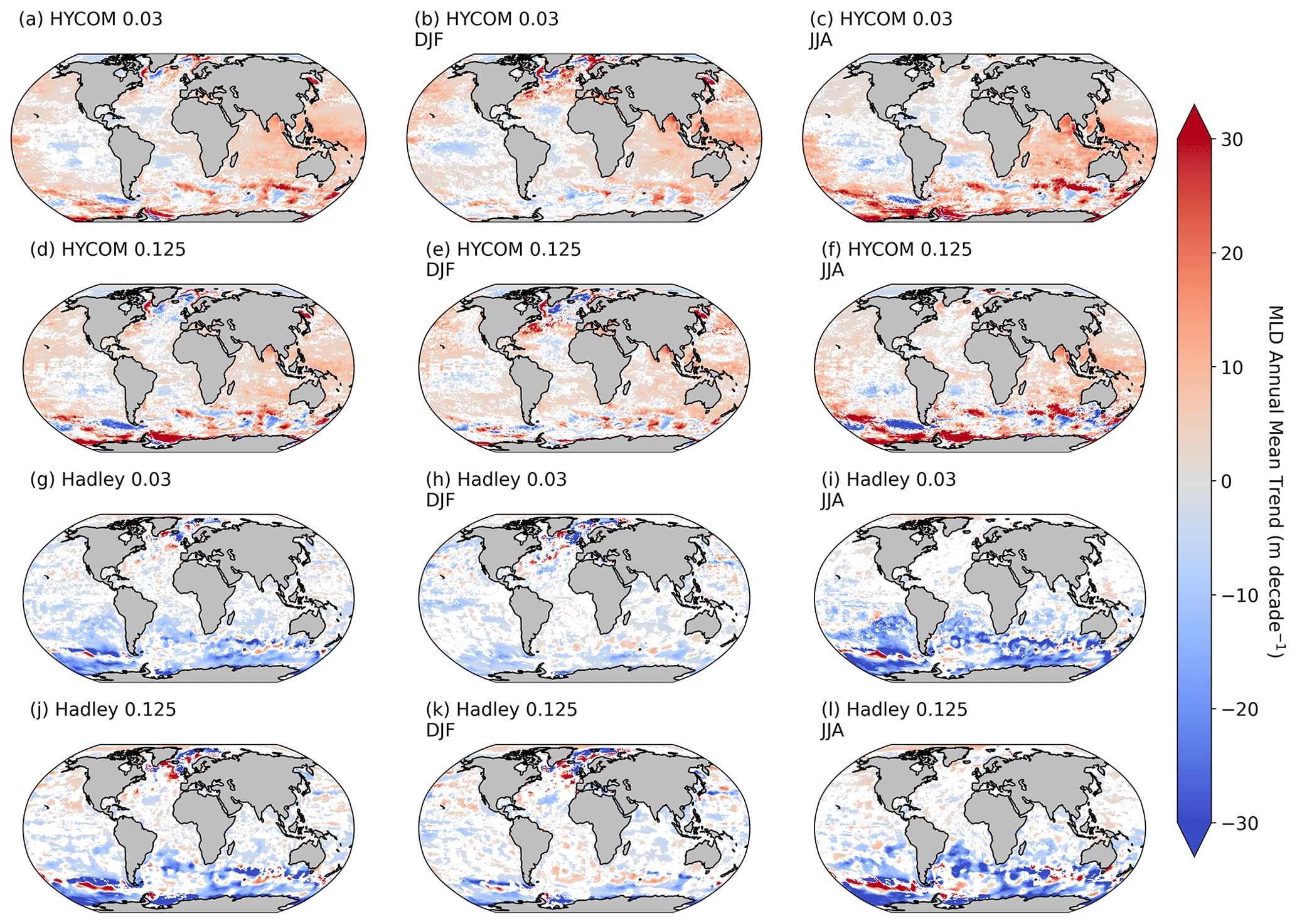
Figure A1The annual mean trends of the different MLD data products HYCOM (a–f) and Hadley (g–l) for the different criteria of Δσ10 m = 0.030 kg m−3 (a–c, g–i) and Δσ10 m = 0.125 kg m−3 (d–f, j–l), averaged for the whole year (a, d, g, j), December to February (b, e, h, k), and June to August (c, f, i, l). Trend analysis performed as described in Ryan-Keogh et al. (2023e).
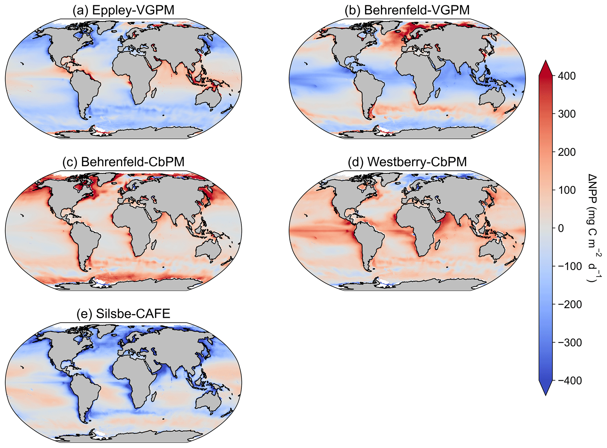
Figure A2The difference in climatological mean [1998–2022] NPPs between the inter-model mean and (a) Eppley-VGPM, (b) Behrenfeld-VGPM, (c) Behrenfeld-CbPM, (d) Westberry-CbPM, and (e) Silsbe-CAFE models.
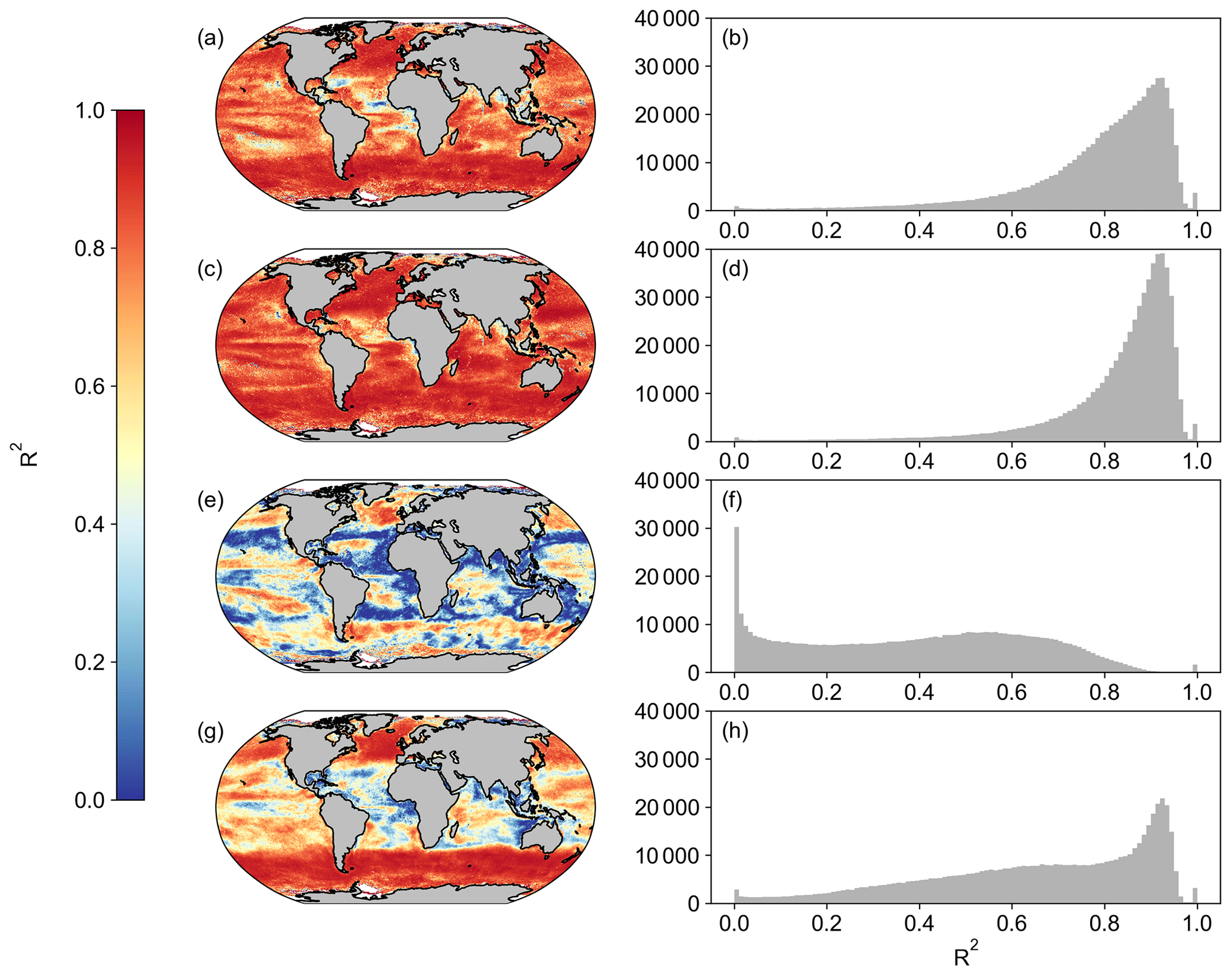
Figure A3Spatial correlation maps and histograms of Pearson's correlation coefficient R2 values between SeaWIFS and OC-CCI for the period of 1 January 1998 to 31 December 2007 for (a, b) Eppley-VGPM, (c, d) Behrenfeld-VGPM, (e, f) Westberry-CbPM, and (g, h) Silsbe-CAFE. Please note that for Westberry-CbPM and Silsbe-CAFE, the MLD product used for SeaWIFS is HYCOM, and the MLD product for OC-CCI is Hadley, both using the Δσ10 m = 0.030 kg m−3 criterion.
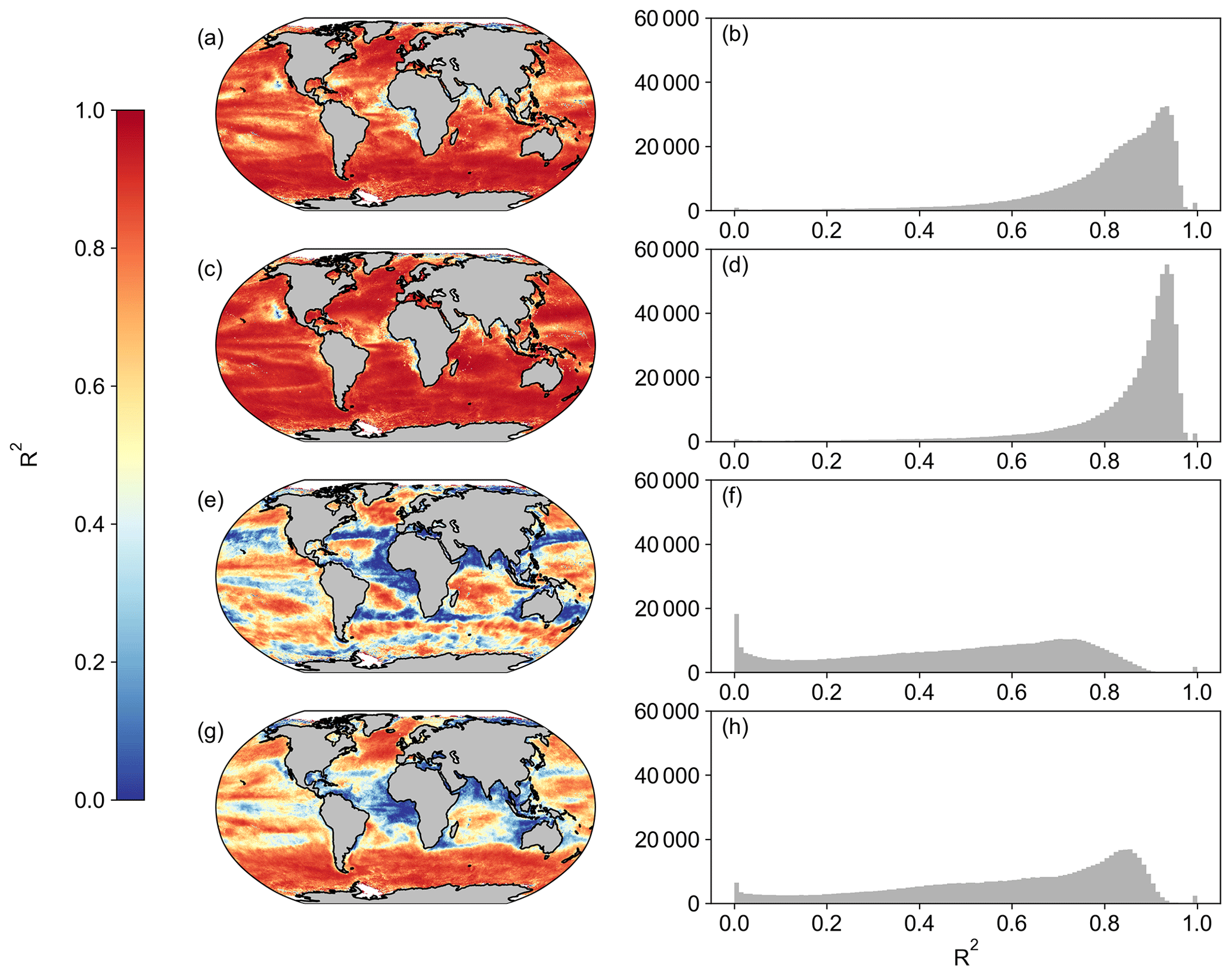
Figure A4Spatial correlation maps and histograms of Pearson's correlation coefficient R2 values between MODIS and OC-CCI for the period of 1 January 2003 to 31 December 2019 for (a, b) Eppley-VGPM, (c, d) Behrenfeld-VGPM, (e, f) Westberry-CbPM, and (g, h) Silsbe-CAFE. Please note that, for Westberry-CbPM and Silsbe-CAFE, the MLD product used for SeaWIFS is HYCOM, and the MLD product for OC-CCI is Hadley, both using the Δσ10 m = 0.030 kg m−3 criterion.
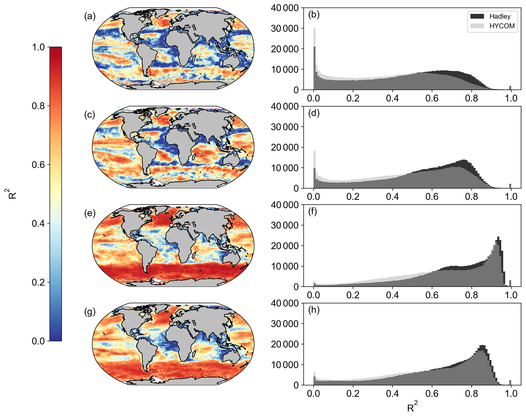
Figure A5Spatial correlation maps and histograms of Pearson's correlation coefficient R2 values between SeaWIFS (a, b, e, f), MODIS (c, d, g, h), and OC-CCI for (a–d) Westberry-CbPM and (e–h) Silsbe-CAFE. Please note that the MLD product used is HYCOM with the Δσ10 m = 0.030 kg m−3 criterion. Included in the histograms are the Pearson's correlation coefficient R2 values using the Hadley MLD data product (in black), as displayed in Figs. A3 and A4.
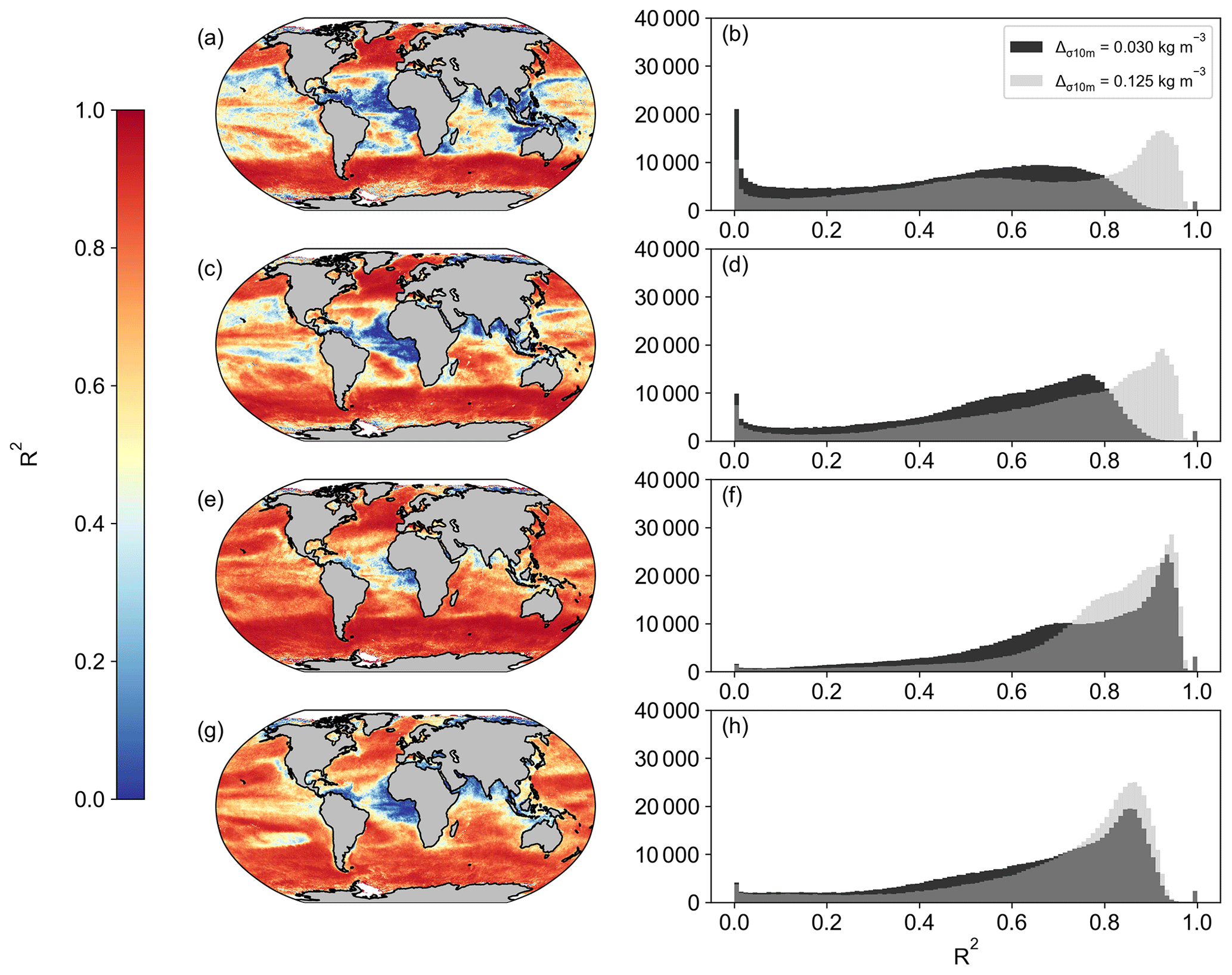
Figure A6Spatial correlation maps and histograms of Pearson's correlation coefficient R2 values using the MLD criterion of Δσ10 m = 0.125 kg m−3 (in grey) for (a, b) Westberry-CbPM SeaWIFS vs. OC-CCI, (c, d) Westberry-CbPM MODIS vs. OC-CCI, (e, f) Silsbe-CAFE SeaWIFS vs. OC-CCI, and (a, b) CAFE MODIS vs. OC-CCI. Included in the histograms are the Pearson's correlation coefficient R2 values using the MLD criterion of Δσ10 m = 0.030 kg m−3 (in black), as displayed in Figs. A3 and A4.
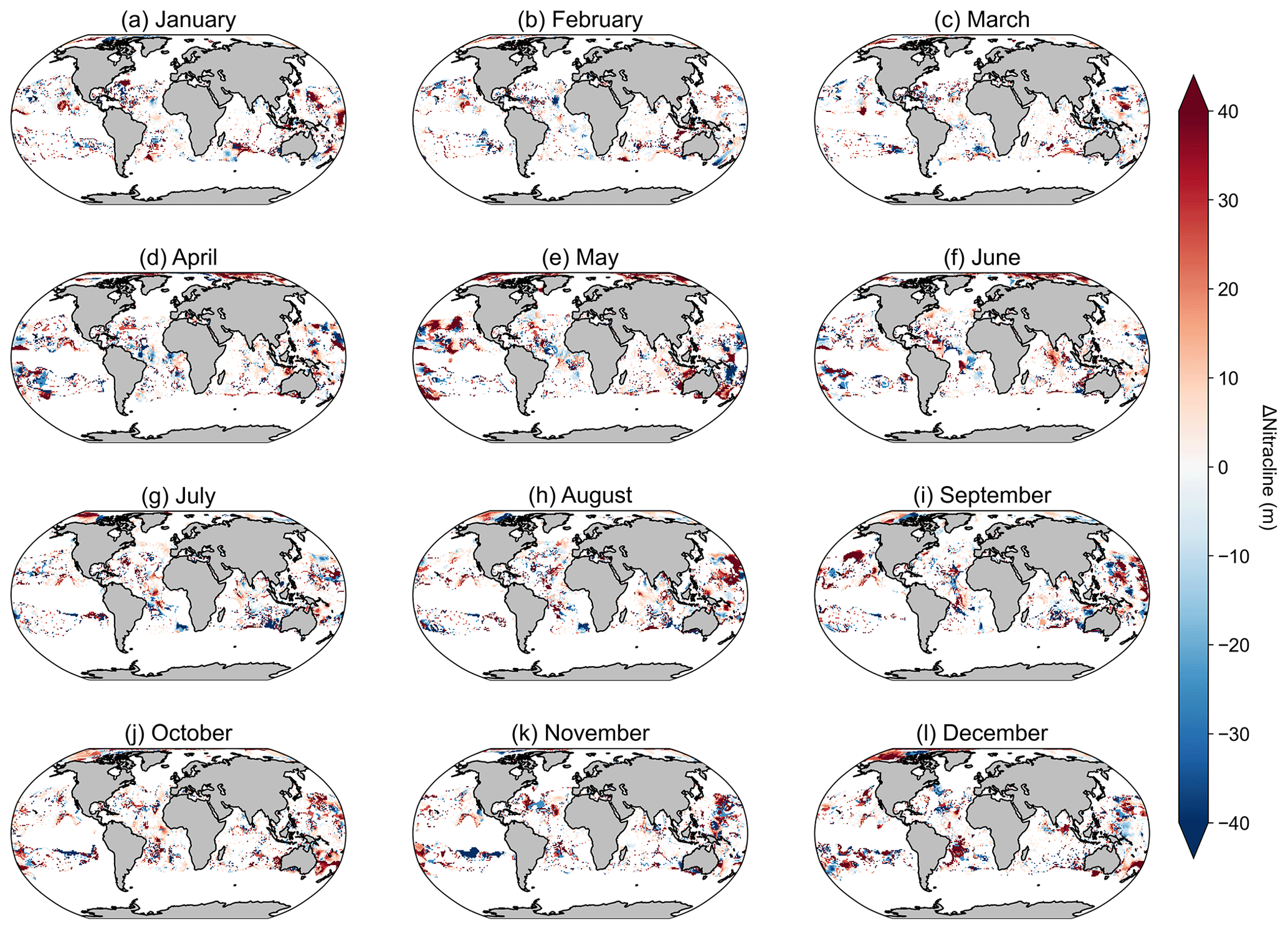
Figure A7Maps of the difference in nitracline depth, where the nitracline depth is calculated as the depth at which nitrate + nitrite is equal to 0.5 µM between monthly WOA2013 and WOA2018.
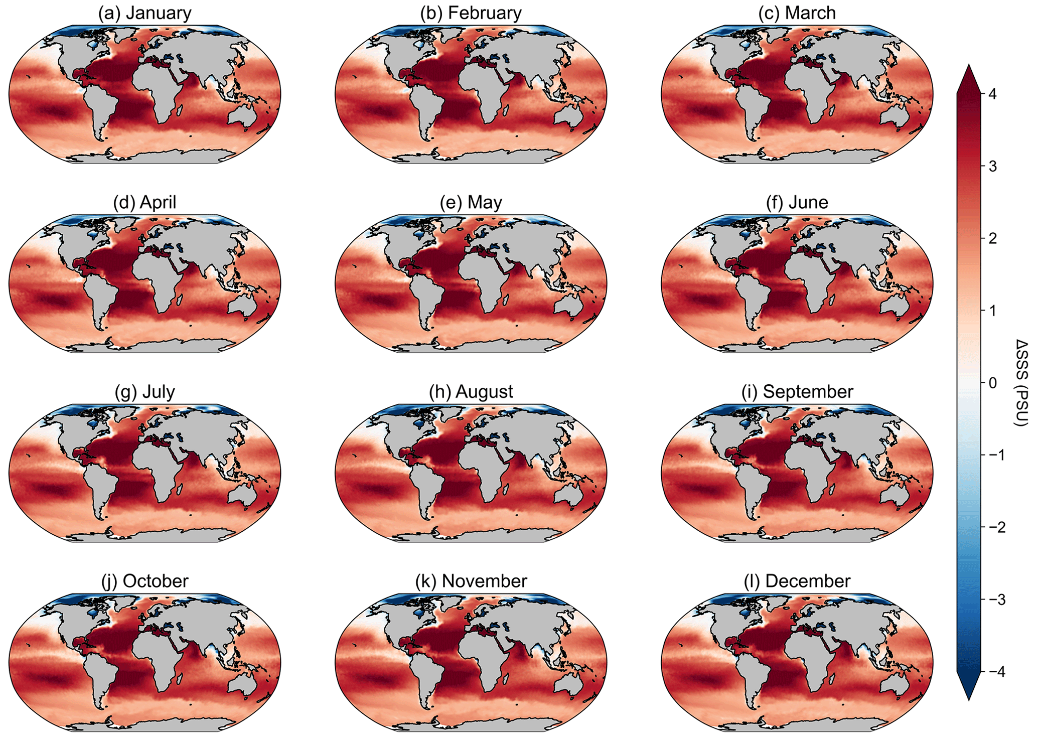
Figure A8Maps of the difference in sea surface salinity (SSS) from the WOA18 monthly climatology and the reference SSS value used in Silsbe et al. (2016) of 32.5 PSU.
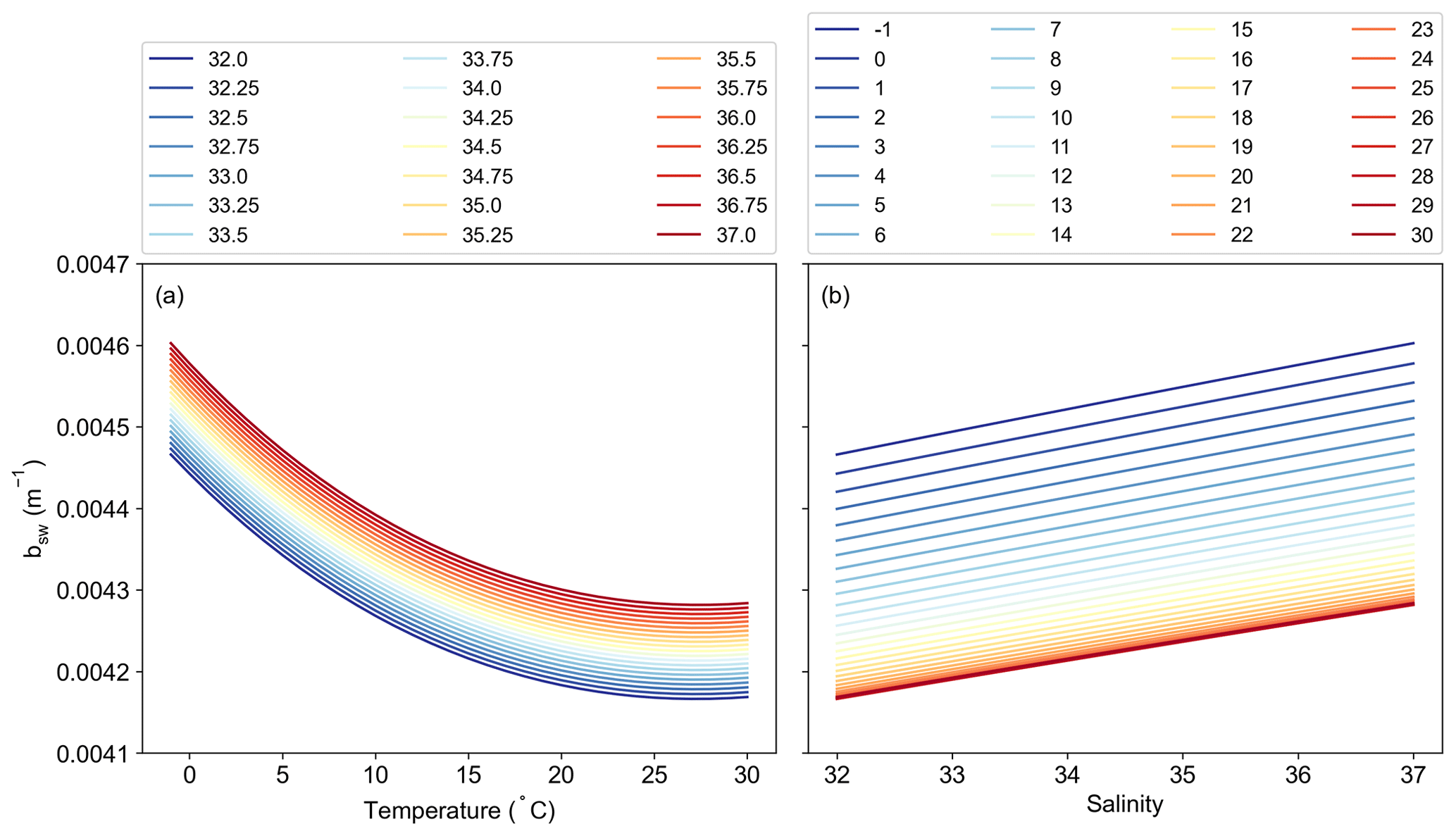
Figure A9Sensitivity analysis of the calculation of the total backscattering of pure seawater (bsw, m−1) as a function of both (a) temperature (∘C) (colour scale = salinity) and (b) salinity (colour scale = temperature, ∘C).
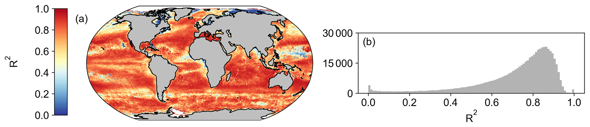
Figure A10A spatial correlation map (a) and a histogram of Pearson's correlation coefficient R2 values (b) between monthly MODIS- and OC-CCI-derived spectral slope of bbp (η) for the period of 1 January 2003 to 31 December 2019.
Conceptualization: TJRK, SJT. Formal analysis: TJRK. Methodology: TJRK. Software: TJRK, NC, TM. Visualization: TJRK. Writing – original draft: TJRK. Writing – reviewing and editing: TJRK, SJT, NC, TM.
The contact author has declared that none of the authors has any competing interests.
Publisher's note: Copernicus Publications remains neutral with regard to jurisdictional claims made in the text, published maps, institutional affiliations, or any other geographical representation in this paper. While Copernicus Publications makes every effort to include appropriate place names, the final responsibility lies with the authors.
We would like to acknowledge the OC-CCI group for providing the satellite data used in this paper. The authors acknowledge their institutional support from the CSIR Parliamentary Grant and the Department of Science and Innovation. We similarly acknowledge the Centre for High-Performance Computing (CSIR-CHPC) for the support and provision of the computational hours required for the analysis of this work. We would like to acknowledge Greg Silsbe for sharing the code for the CAFE algorithm.
This paper was edited by Salvatore Marullo and reviewed by Toby Westberry and one anonymous referee.
ACRI-ST: GlobColour data, http://globcolour.info, last access: 1 September 2023.
Antoine, D. and Morel, A.: Oceanic primary production: 1. Adaptation of a spectral light-photosynthesis model in view of application to satellite chlorophyll observations, Global Biogeochem. Cy., 10, 43–55, https://doi.org/10.1029/95GB02831, 1996.
Antoine, D., André, J.-M., and Morel, A.: Oceanic primary production: 2. Estimation at global scale from satellite (Coastal Zone Color Scanner) chlorophyll, Global Biogeochem. Cy., 10, 57–69, https://doi.org/10.1029/95GB02832, 1996.
Behrenfeld, M. J. and Falkowski, P. G.: Photosynthetic rates derived from satellite-based chlorophyll concentration, Limnol. Oceanogr., 42, 1–20, https://doi.org/10.4319/lo.1997.42.1.0001, 1997.
Behrenfeld, M. J., Boss, E., Siegel, D. A., and Shea, D. M.: Carbon-based ocean productivity and phytoplankton physiology from space, Global Biogeochem. Cy., 19, GB1006–GB1006, https://doi.org/10.1029/2004GB002299, 2005.
Behrenfeld, M. J., O'Malley, R. T., Siegel, D. A., McClain, C. R., Sarmiento, J. L., Feldman, G. C., Milligan, A. J., Falkowski, P. G., Letelier, R. M., and Boss, E. S.: Climate-driven trends in contemporary ocean productivity, Nature, 444, 752–755, https://doi.org/10.1038/nature05317, 2006.
Boalch, G. T.: Changes in the phytoplankton of the western English Channel in recent years, British Phycological J., 22, 225–235, https://doi.org/10.1080/00071618700650291, 1987.
Bopp, L., Resplandy, L., Orr, J. C., Doney, S. C., Dunne, J. P., Gehlen, M., Halloran, P., Heinze, C., Ilyina, T., Séférian, R., Tjiputra, J., and Vichi, M.: Multiple stressors of ocean ecosystems in the 21st century: projections with CMIP5 models, Biogeosciences, 10, 6225–6245, https://doi.org/10.5194/bg-10-6225-2013, 2013.
Boutin, J., Reul, N., Koehler, J., Martin, A., Catany, R., Guimbard, S., Rouffi, F., Vergely, J. L., Arias, M., Chakroun, M., Corato, G., Estella-Perez, V., Hasson, A., Josey, S., Khvorostyanov, D., Kolodziejczyk, N., Mignot, J., Olivier, L., Reverdin, G., Stammer, D., Supply, A., Thouvenin-Masson, C., Turiel, A., Vialard, J., Cipollini, P., Donlon, C., Sabia, R., and Mecklenburg, S.: Satellite-Based Sea Surface Salinity Designed for Ocean and Climate Studies, J. Geophys. Res.-Oceans, 126, e2021JC017676-e2021JC017676, https://doi.org/10.1029/2021JC017676, 2021.
Boyd, P. W., Lennartz, S. T., Glover, D. M., and Doney, S. C.: Biological ramifications of climate-change-mediated oceanic multi-stressors, Nat. Clim. Change, 5, 71–79, https://doi.org/10.1038/nclimate2441, 2015.
Brewin, R. J. W., Sathyendranath, S., Müller, D., Brockmann, C., Deschamps, P.-Y., Devred, E., Doerffer, R., Fomferra, N., Franz, B., Grant, M., Groom, S., Horseman, A., Hu, C., Krasemann, H., Lee, Z., Maritorena, S., Mélin, F., Peters, M., Platt, T., Regner, P., Smyth, T., Steinmetz, F., Swinton, J., Werdell, J., and White, G. N.: The Ocean Colour Climate Change Initiative: III. A round-robin comparison on in-water bio-optical algorithms, Remote Sens. Environ., 162, 271–294, https://doi.org/10.1016/j.rse.2013.09.016, 2015.
Buitenhuis, E. T., Hashioka, T., and Quéré, C. Le: Combined constraints on global ocean primary production using observations and models, Global Biogeochem. Cy., 27, 847–858, https://doi.org/10.1002/gbc.20074, 2013.
Campbell, J., Antoine, D., Armstrong, R., Arrigo, K., Balch, W., Barber, R., Behrenfeld, M., Bidigare, R., Bishop, J., Carr, M.-E., Esaias, W., Falkowski, P., Hoepffner, N., Iverson, R., Kiefer, D., Lohrenz, S., Marra, J., Morel, A., Ryan, J., Vedernikov, V., Waters, K., Yentsch, C., and Yoder, J.: Comparison of algorithms for estimating ocean primary production from surface chlorophyll, temperature, and irradiance, Global Biogeochem. Cy., 16, 9–1-9–15, https://doi.org/10.1029/2001GB001444, 2002.
Carr, M.-E., Friedrichs, M. A. M., Schmeltz, M., Noguchi Aita, M., Antoine, D., Arrigo, K. R., Asanuma, I., Aumont, O., Barber, R., Behrenfeld, M., Bidigare, R., Buitenhuis, E. T., Campbell, J., Ciotti, A., Dierssen, H., Dowell, M., Dunne, J., Esaias, W., Gentili, B., Gregg, W., Groom, S., Hoepffner, N., Ishizaka, J., Kameda, T., Le Quéré, C., Lohrenz, S., Marra, J., Mélin, F., Moore, K., Morel, A., Reddy, T. E., Ryan, J., Scardi, M., Smyth, T., Turpie, K., Tilstone, G., Waters, K., and Yamanaka, Y.: A comparison of global estimates of marine primary production from ocean color, Deep-Sea Res. Pt. II, 53, 741–770, https://doi.org/10.1016/j.dsr2.2006.01.028, 2006.
Chavez, F. P., Messié, M., and Pennington, J. T.: Marine Primary Production in Relation to Climate Variability and Change, Annu. Rev. Mar. Sci., 3, 227–260, https://doi.org/10.1146/annurev.marine.010908.163917, 2010.
de Boyer Montégut, C., Madec, G., Fischer, A. S., Lazar, A., and Iudicone, D.: Mixed layer depth over the global ocean: An examination of profile data and a profile-based climatology, J. Geophys. Res.-Oceans, 109, https://doi.org/10.1029/2004JC002378, 2004.
Eppley, R. W.: Temperature and phytoplankton growth in the sea, Fishery B.-NOAA, 70, 1063–1085, 1972.
Fay, A. R. and McKinley, G. A.: Global open-ocean biomes: mean and temporal variability, Earth Syst. Sci. Data, 6, 273–284, https://doi.org/10.5194/essd-6-273-2014, 2014.
IPCC: Climate Change 2014: Impacts, Adaptation, and Vulnerability. Part A: Global and Sectoral Aspects. Contribution of Working Group II to the Fifth Assessment Report of the Intergovernmental Panel on Climate Change, edited by: Field, C. B., Barros, V. R., Dokken, D. J., Mach, K. J., Mastrandrea, M. D., Bilir, T. E., Chatterjee, M., Ebi, K. L., Estrada, Y. O., Genova, R. C., Girma, B., Kissel, E. S., Levy, A. N., MacCracken, S., Mastrandrea, P. R., and White, L. L., Cambridge University Press, Cambridge, United Kingdom and New York, NY, USA, 1132 pp., 2014.
Field, C. B., Behrenfeld, M. J., Randerson, J. T., and Falkowski, P.: Primary production of the biosphere: Integrating terrestrial and oceanic components, Science (1979), 281, 237–240, https://doi.org/10.1126/science.281.5374.237, 1998.
Friedrichs, M. A. M., Carr, M.-E., Barber, R. T., Scardi, M., Antoine, D., Armstrong, R. A., Asanuma, I., Behrenfeld, M. J., Buitenhuis, E. T., Chai, F., Christian, J. R., Ciotti, A. M., Doney, S. C., Dowell, M., Dunne, J., Gentili, B., Gregg, W., Hoepffner, N., Ishizaka, J., Kameda, T., Lima, I., Marra, J., Mélin, F., Moore, J. K., Morel, A., O'Malley, R. T., O'Reilly, J., Saba, V. S., Schmeltz, M., Smyth, T. J., Tjiputra, J., Waters, K., Westberry, T. K., and Winguth, A.: Assessing the uncertainties of model estimates of primary productivity in the tropical Pacific Ocean, J. Marine Syst., 76, 113–133, https://doi.org/10.1016/j.jmarsys.2008.05.010, 2009.
Garcia, H., Weathers, K., Paver, C., Smolyar, I., Boyer, T., Locarnini, M., Zweng, M., Mishonov, A., Baranova, O., Seidov, D., and Reagan, J.: World Ocean Atlas 2018, Vol. 4, Dissolved Inorganic Nutrients (phosphate, nitrate and nitrate+nitrite, silicate), Technical Editor: Mishonov, A., NOAA Atlas NESDIS 84, 35 pp., https://www.ncei.noaa.gov/access/world-ocean-atlas-2018/ (last access: 1 September 2023), 2019.
Garver, S. A. and Siegel, D. A.: Inherent optical property inversion of ocean color spectra and its biogeochemical interpretation: 1. Time series from the Sargasso Sea, J. Geophys. Res.-Oceans, 102, 18607–18625, https://doi.org/10.1029/96JC03243, 1997.
Good, S. A., Martin, M. J., and Rayner, N. A.: EN4: Quality controlled ocean temperature and salinity profiles and monthly objective analyses with uncertainty estimates, J. Geophys. Res.-Oceans, 118, 6704–6716, https://doi.org/10.1002/2013JC009067, 2013.
Gregg, W. W. and Rousseaux, C. S.: Global ocean primary production trends in the modern ocean color satellite record (1998–2015), Environ. Res. Lett., 14, 124011, https://doi.org/10.1088/1748-9326/ab4667, 2019.
Gruber, N., Gloor, M., Mikaloff Fletcher, S. E., Doney, S. C., Dutkiewicz, S., Follows, M. J., Gerber, M., Jacobson, A. R., Joos, F., Lindsay, K., Menemenlis, D., Mouchet, A., Müller, S. A., Sarmiento, J. L., and Takahashi, T.: Oceanic sources, sinks, and transport of atmospheric CO2, Global Biogeochem. Cy., 23, GB1005, https://doi.org/10.1029/2008GB003349, 2009.
Haumann, F. A., Gruber, N., and Münnich, M.: Sea-Ice Induced Southern Ocean Subsurface Warming and Surface Cooling in a Warming Climate, AGU Advances, 1, e2019AV000132, https://doi.org/10.1029/2019AV000132, 2020.
Henson, S. A., Dunne, J. P., and Sarmiento, J. L.: Decadal variability in North Atlantic phytoplankton blooms, J. Geophys. Res.-Oceans, 114, C04013, https://doi.org/10.1029/2008JC005139, 2009.
Henson, S. A., Sanders, R., Madsen, E., Morris, P. J., Le Moigne, F., and Quartly, G. D.: A reduced estimate of the strength of the ocean's biological carbon pump, Geophys. Res. Lett., 38, L04606, https://doi.org/10.1029/2011GL046735, 2011.
Johnson, K. S. and Bif, M. B.: Constraint on net primary productivity of the global ocean by Argo oxygen measurements, Nat. Geosci., 14, 769–774, https://doi.org/10.1038/s41561-021-00807-z, 2021.
Kulk, G., Platt, T., Dingle, J., Jackson, T., Jönsson, B. F., Bouman, H. A., Babin, M., Brewin, R. J. W., Doblin, M., Estrada, M., Figueiras, F. G., Furuya, K., González-Benítez, N., Gudfinnsson, H. G., Gudmundsson, K., Huang, B., Isada, T., Kovač, Ž., Lutz, V. A., Marañón, E., Raman, M., Richardson, K., Rozema, P. D., Poll, W. H. van de, Segura, V., Tilstone, G. H., Uitz, J., Dongen-Vogels, V. V, Yoshikawa, T., and Sathyendranath, S.: Primary Production, an Index of Climate Change in the Ocean: Satellite-Based Estimates over Two Decades, Remote Sens., 12, 826, https://doi.org/10.3390/rs12050826, 2020.
Lee, Z., Carder, K. L., and Arnone, R. A.: Deriving inherent optical properties from water color: a multiband quasi-analytical algorithm for optically deep waters, Appl. Optics, 41, 5755–5772, https://doi.org/10.1364/AO.41.005755, 2002.
Lee, Z., Marra, J., Perry, M. J., and Kahru, M.: Estimating oceanic primary productivity from ocean color remote sensing: A strategic assessment, J. Marine Syst., 149, 50–59, https://doi.org/10.1016/j.jmarsys.2014.11.015, 2015.
Longhurst, A., Sathyendranath, S., Platt, T., and Caverhill, C.: An Estimate of Global Primary Production in the Ocean from Satellite Radiometer Data, J. Plankton Res., 17, 1245–1271, 1995.
Lurin, B.: Global terrestrial net primary production, Glob. Change News I. (IGPB), 19, 6–8, 1994.
Maritorena, S., Siegel, D. A., and Peterson, A. R.: Optimization of a semianalytical ocean color model for global-scale applications, Appl. Optics, 41, 2705–2714, https://doi.org/10.1364/AO.41.002705, 2002.
Mikaloff Fletcher, S. E., Gruber, N., Jacobson, A. R., Gloor, M., Doney, S. C., Dutkiewicz, S., Gerber, M., Follows, M., Joos, F., Lindsay, K., Menemenlis, D., Mouchet, A., Müller, S. A., and Sarmiento, J. L.: Inverse estimates of the oceanic sources and sinks of natural CO2 and the implied oceanic carbon transport, Global Biogeochem. Cy., 21, GB1010, https://doi.org/10.1029/2006GB002751, 2007.
Monteiro, P. M. S., Boyd, P., and Bellerby, R.: Role of the seasonal cycle in coupling climate and carbon cycling in the subantarctic zone, Eos T. Am. Geophys. Un., 92, 235–236, https://doi.org/10.1029/2011EO280007, 2011.
National Centers for Environmental Information: Daily L4 Optimally Interpolated SST (OISST) In situ and AVHRR Analysis, Ver. 2.0., National Centers for Environmental Information [data set], https://doi.org/10.5067/GHAAO-4BC02, 2023.
O'Malley, R.: Ocean Productivity – Oregon State University, http://orca.science.oregonstate.edu/npp_products.php, last access: 1 September 2023.
Pitarch, J., Bellacicco, M., Organelli, E., Volpe, G., Colella, S., Vellucci, V., and Marullo, S.: Retrieval of Particulate Backscattering Using Field and Satellite Radiometry: Assessment of the QAA Algorithm, Remote Sens.-Basel, 12, 77, https://doi.org/10.3390/rs12010077, 2019.
Polovina, J. J., Dunne, J. P., Woodworth, P. A., and Howell, E. A.: Projected expansion of the subtropical biome and contraction of the temperate and equatorial upwelling biomes in the North Pacific under global warming, ICES J. Mar. Sci., 68, 986–995, https://doi.org/10.1093/icesjms/fsq198, 2011.
Racault, M.-F., Sathyendranath, S., and Platt, T.: Impact of missing data on the estimation of ecological indicators from satellite ocean-colour time-series, Remote Sens. Environ., 152, 15–28, https://doi.org/10.1016/j.rse.2014.05.016, 2014.
Rhein, M., Rintoul, S. R., Aoki, S., Campos, E., Chambers, D., Feely, R., Gulev, S., Johnson, G. C., Josey, S., and Kostianoy, A.: Observations: Ocean, in: Climate Change 2013: The Physical Science Basis. Contribution of Working Group I to the Fifth Assessment Report of the Intergovernmental Panel on Climate Change, edited by: Stocker, T. F., Qin, D., Plattner, G.-K., Tignor, M., Allen, S. K., Boschung, J., Nauels, A., Xia, Y., Bex, V., and Midgley, P. M., Cambridge University Press, Cambridge, United Kingdom and New York, NY, USA, 255–316, https://doi.org/10.1017/CBO9781107415324.010, 2013.
Ryan-Keogh, T., Thomalla, S., Chang, N., and Moalusi, T.: Net primary production from the Behrenfeld-CbPM, Westberry-CbPM and Silsbe-CAFE algorithms – HADLEY MLD 0.125 Criterion, Zenodo [data set], https://doi.org/10.5281/ZENODO.8320875, 2023a.
Ryan-Keogh, T., Thomalla, S., Chang, N., and Moalusi, T.: Net primary production from the Behrenfeld-CbPM, Westberry-CbPM and Silsbe-CAFE algorithms – HYCOM MLD 0.030 Criterion, Zenodo [data set], https://doi.org/10.5281/ZENODO.8320872, 2023b.
Ryan-Keogh, T., Thomalla, S., Chang, N., and Moalusi, T.: Net primary production from the Behrenfeld-CbPM, Westberry-CbPM and Silsbe-CAFE algorithms – HYCOM MLD 0.125 Criterion, Zenodo [data set], https://doi.org/10.5281/ZENODO.8318272, 2023c.
Ryan-Keogh, T., Thomalla, S., Chang, N., and Moalusi, T.: Net primary production from the Eppley-VGPM, Behrenfeld-VGPM, Behrenfeld-CbPM, Westberry-CbPM and Silsbe-CAFE algorithms, Zenodo [data set], https://doi.org/10.5281/ZENODO.8314348, 2023d.
Ryan-Keogh, T. J., Thomalla, S. J., Monteiro, P. M. S., and Tagliabue, A.: Multidecadal trend of increasing iron stress in Southern Ocean phytoplankton, Science, 379, https://doi.org/10.1126/science.abl5237, 2023.
Saba, V. S., Friedrichs, M. A. M., Carr, M.-E., Antoine, D., Armstrong, R. A., Asanuma, I., Aumont, O., Bates, N. R., Behrenfeld, M. J., Bennington, V., Bopp, L., Bruggeman, J., Buitenhuis, E. T., Church, M. J., Ciotti, A. M., Doney, S. C., Dowell, M., Dunne, J., Dutkiewicz, S., Gregg, W., Hoepffner, N., Hyde, K. J. W., Ishizaka, J., Kameda, T., Karl, D. M., Lima, I., Lomas, M. W., Marra, J., McKinley, G. A., Mélin, F., Moore, J. K., Morel, A., O'Reilly, J., Salihoglu, B., Scardi, M., Smyth, T. J., Tang, S., Tjiputra, J., Uitz, J., Vichi, M., Waters, K., Westberry, T. K., and Yool, A.: Challenges of modeling depth-integrated marine primary productivity over multiple decades: A case study at BATS and HOT, Global Biogeochem. Cy., 24, GB3020, https://doi.org/10.1029/2009GB003655, 2010.
Saba, V. S., Friedrichs, M. A. M., Antoine, D., Armstrong, R. A., Asanuma, I., Behrenfeld, M. J., Ciotti, A. M., Dowell, M., Hoepffner, N., Hyde, K. J. W., Ishizaka, J., Kameda, T., Marra, J., Mélin, F., Morel, A., O'Reilly, J., Scardi, M., Smith Jr., W. O., Smyth, T. J., Tang, S., Uitz, J., Waters, K., and Westberry, T. K.: An evaluation of ocean color model estimates of marine primary productivity in coastal and pelagic regions across the globe, Biogeosciences, 8, 489–503, https://doi.org/10.5194/bg-8-489-2011, 2011.
Salgado-Hernanz, P. M., Racault, M.-F., Font-Muñoz, J. S., and Basterretxea, G.: Trends in phytoplankton phenology in the Mediterranean Sea based on ocean-colour remote sensing, Remote Sens Environ, 221, 50–64, https://doi.org/10.1016/j.rse.2018.10.036, 2019.
Sallée, J.-B., Pellichero, V., Akhoudas, C., Pauthenet, E., Vignes, L., Schmidtko, S., Garabato, A. N., Sutherland, P., and Kuusela, M.: Summertime increases in upper-ocean stratification and mixed-layer depth, Nature, 591, 592–598, https://doi.org/10.1038/s41586-021-03303-x, 2021.
Sathyendranath, S., Brewin, R. J. W., Brockmann, C., Brotas, V., Calton, B., Chuprin, A., Cipollini, P., Couto, A. B., Dingle, J., Doerffer, R., Donlon, C., Dowell, M., Farman, A., Grant, M., Groom, S., Horseman, A., Jackson, T., Krasemann, H., Lavender, S., Martinez-Vicente, V., Mazeran, C., Mélin, F., Moore, T. S., Müller, D., Regner, P., Roy, S., Steele, C. J., Steinmetz, F., Swinton, J., Taberner, M., Thompson, A., Valente, A., Zühlke, M., Brando, V. E., Feng, H., Feldman, G., Franz, B. A., Frouin, R., Gould, R. W., Hooker, S. B., Kahru, M., Kratzer, S., Mitchell, B. G., Muller-Karger, F. E., Sosik, H. M., Voss, K. J., Werdell, J., and Platt, T.: An Ocean-Colour Time Series for Use in Climate Studies: The Experience of the Ocean-Colour Climate Change Initiative (OC-CCI), Sensors, 19, 4285, https://doi.org/10.3390/s19194285, 2019a.
Sathyendranath, S., Platt, T., Brewin, R. J. W., and Jackson, T.: Primary Production Distribution?, in: Encyclopedia of Ocean Sciences (Third Edition), edited by: Cochran, J. K., Bokuniewicz, H. J., and Yager, P. L., Academic Press, Oxford, 635–640, https://doi.org/10.1016/B978-0-12-409548-9.04304-9, 2019b.
Silsbe, G. M., Behrenfeld, M. J., Halsey, K. H., Milligan, A. J., and Westberry, T. K.: The CAFE model: A net production model for global ocean phytoplankton, Global Biogeochem. Cy., 30, 1756–1777, https://doi.org/10.1002/2016GB005521, 2016.
Suga, T., Motoki, K., Aoki, Y., and Macdonald, A. M.: The North Pacific Climatology of Winter Mixed Layer and Mode Waters, J. Phys. Oceanogr., 34, 3–22, https://doi.org/10.1175/1520-0485(2004)034<0003:TNPCOW>2.0.CO;2, 2004.
Summer, U. and Lengfeller, K.: Climate change and the timing, magnitude, and composition of the phytoplankton spring bloom, Global Change Biol., 14, 1199–1208, https://doi.org/10.1111/j.1365-2486.2008.01571.x, 2008.
Tagliabue, A., Kwiatkowski, L., Bopp, L., Butenschön, M., Cheung, W., Lengaigne, M., and Vialard, J.: Persistent Uncertainties in Ocean Net Primary Production Climate Change Projections at Regional Scales Raise Challenges for Assessing Impacts on Ecosystem Services, https://doi.org/10.3389/fclim.2021.738224, 2021.
Tao, Z., Wang, Y., Ma, S., Lv, T., and Zhou, X.: A Phytoplankton Class-Specific Marine Primary Productivity Model Using MODIS Data, IEEE J. Sel. Top. Appl., 10, 5519–5528, https://doi.org/10.1109/JSTARS.2017.2747770, 2017.
Tilstone, G. H., Land, P. E., Pardo, S., Kerimoglu, O., and Van der Zande, D.: Threshold indicators of primary production in the north-east Atlantic for assessing environmental disturbances using 21 years of satellite ocean colour, Sci. Total Environ., 854, 158757, https://doi.org/10.1016/j.scitotenv.2022.158757, 2023.
Westberry, T., Behrenfeld, M. J., Siegel, D. A., and Boss, E.: Carbon-based primary productivity modeling with vertically resolved photoacclimation, Global Biogeochem. Cy., 22, GB2024, https://doi.org/10.1029/2007GB003078, 2008.
Westberry, T. K., Silsbe, G. M., and Behrenfeld, M. J.: Gross and net primary production in the global ocean: An ocean color remote sensing perspective, Earth-Sci. Rev., 237, 104322, https://doi.org/10.1016/j.earscirev.2023.104322, 2023.
Zhang, X. and Hu, L.: Estimating scattering of pure water from density fluctuation of the refractive index, Opt. Express, 17, 1671–1678, https://doi.org/10.1364/OE.17.001671, 2009.
Zhuang, J., dussin, raphael, Huard, D., Bourgault, P., Banihirwe, A., Raynaud, S., Malevich, B., Schupfner, M., Filipe, Levang, S., Jüling, A., Almansi, M., RichardScottOZ, RondeauG, Rasp, S., Smith, T. J., Stachelek, J., Plough, M., Pierre, Bell, R., and Li, X.: pangeo-data/xESMF: v0.7.1, Zenodo [code], https://doi.org/10.5281/ZENODO.7800141, 2023.