2.1 TM5-MP

The global chemical transport model TM5-MP (Tracer Model 5, Massively Parallel version; Krol et al., 2005; Huijnen et al., 2010; van Noije et al., 2014, 2021; Williams et al., 2017) has been applied in this study. It is driven by the input meteorological fields which are produced from ERA-Interim reanalysis datasets provided by the ECMWF (European Centre for Medium-range Weather Forecasts; Dee et al., 2011). The model accounts for gas-phase, aqueous-phase and heterogeneous chemistry. The gas-phase chemistry scheme is a modified version of the CB05 carbon bond mechanism (Yarwood et al., 2005), which was described in detail in Williams et al. (2017).

TM5-MP predicts aerosol dynamic processes using the two-moment modal model M7 (Vignati et al., 2004), which includes seven log-normally distributed modes with four water-soluble modes (nucleation, Aitken, accumulation and coarse) and three insoluble modes (Aitken, accumulation and coarse). Each mode corresponds to a specific dry diameter range: nucleation mode is less than 10 nm, Aitken mode ranges from 10 to 100 nm, accumulation mode from 100 nm to 1 µm and coarse mode is greater than 1 µm.

The current version of TM5-MP incorporates SOA into four soluble modes and the insoluble Aitken mode, resulting in a comprehensive aerosol model including SOA, sulfate, ammonium, nitrate, methane sulfonic acid (MSA), primary organic aerosol, black carbon, sea salt and mineral dust (Bergman et al., 2022). Isoprene and monoterpenes, acting as gaseous precursors of SOA, are from natural emissions calculated by MEGANv2.1 (Model of Emissions of Gases and Aerosols from Nature version 2.1; Guenther et al., 2012; Sindelarova et al., 2014) and biomass burning emissions based on van Marle et al. (2017). The isoprene and monoterpenes can be oxidized by OH and O₃ in the air to form extremely low-volatility organic compounds (ELVOCs) and semi-volatile organic compounds (SVOCs). The ELVOCs first participate in new particle formation and the rest condense onto existing aerosol particles. The SVOCs only condense due to their higher volatilities. The particle formation and condensation processes occur within one time step, so the transport of ELVOCs and SVOCs is not simulated. More details are described in Bergman et al. (2022).

The dust emissions are calculated online based on the method introduced in Tegen et al. (2002) and extended by Heinhold et al. (2007). New dust emission parameterization methods have also been developed (e.g., Leung et al., 2023) but have not been implemented into the current TM5-MP version. Only the features related to this study are described here. Firstly, we proportion dust emissions to the non-vegetated area within a grid cell, which is determined by the vegetation cover data (see Eq. 1 in Tegen et al., 2002). When dominated by shrubs, we apply the maximum annual vegetation cover, whereas when grass dominates, we use the monthly value. Secondly, Tegen et al. (2002) simulated the potential maximum extent of lakes, and determined preferential dust source regions from the difference between the maximum areas and actual present-day lakes. These regions are assumed to contain silt aggregates composed of finer particles with a median particle radius of 15 µm in the Northern Hemisphere (NH) and 27 µm in the Southern Hemisphere (SH), requiring a smaller wind stress threshold to lift, which is 30 and 20 cm s⁻¹ in the NH and SH, respectively. Moreover, the ratio between the vertical dust flux and horizontal soil particle flux is also assumed to be the largest among all regions, which is set to 10⁻⁵ cm⁻¹. All these factors have determined high dust emission fluxes over the preferential source regions. However, we should note that in TM5-MP, the threshold wind stress (u_min) is set to 13.75 cm s⁻¹ for all kinds of land covers, which reduce further when the cultivation cover exceeds 8% and the grid cell is dominated by either grass or shrub. For more details, see Tegen et al. (2002) and van Noije et al. (2021).

2.2 Model setup

Simulations have been conducted for five different cases: a PI control run (pi_ctrl), a PI run with the default TM5-MP configuration (pi_orig), a PI control run excluding anthropogenic emissions (pi_zero), a standard MH run (mh) and an MH run incorporating a Green Sahara and reduced dust (mh_gsrd) (Table 1). The model configuration for each case will be detailed subsequently. All simulations applied a horizontal resolution of 3^∘ in longitude and 2^∘ in latitude with 34 vertical hybrid-sigma levels. The base time step was set to 1 h. Each simulation ran for 2 years, with the first year serving as the spin-up and the results being analyzed from the second year. The 1-year spin-up in TM5-MP simulations was also applied in previous studies (e.g., Williams et al., 2017; Myriokefalitakis et al., 2020) and was validated here in a 12-year simulation test case (see Fig. S1 in the Supplement).

Table 1Model configurations of the simulation cases pi_ctrl, pi_orig, pi_zero, mh and mh_gsrd. The number 1850 and 2009 show the years that the input data are from. Here lsm means land–sea mask, PD is present-day lsm and MH is mid-Holocene lsm with paleo-lakes switched on as water surface. For vegetation, pi_mean, mh_mean and mh_gsrd_mean represent the 10-year mean of the simulation data from PI, MH and MH_gsrd cases in Lu et al. (2018), respectively. For the emissions of isoprene and monoterpenes, as well as the fraction of absorbed photosynthetically active radiation (FPAR), pi_mean, mh_mean and mh_gsrd_mean represent that the data are derived from their corresponding vegetation data. The “original” means using default original TM5-MP input data. The mixing ratios of CO₂ and CH₄ are fixed to 265.4 ppmv and 597.0 ppbv, respectively, for MH cases.

Download Print Version | Download XLSX

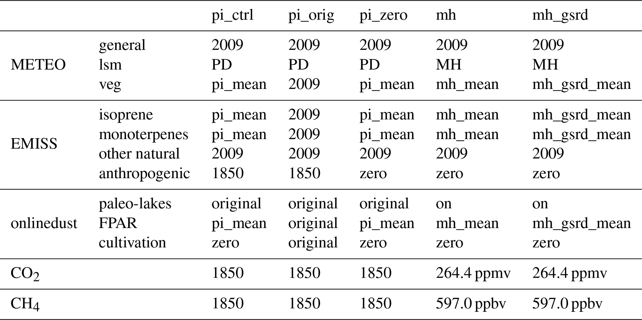
In all five simulation cases, the input meteorological data for spin-up simulations were derived from the year 2008, and the year 2009 was used for subsequent-year simulations, facilitating a focus on comparisons between individual cases. The vegetation cover data for pi_ctrl, mh and mh_gsrd cases were derived from respective PI, MH and MH_gsrd simulation results in Lu et al. (2018).

The anthropogenic emissions are set to 1850 levels for pi_orig and pi_ctrl cases and are switched off for mh and mh_gsrd cases. The natural emissions in 2009 are applied in pi_ctrl, pi_orig, mh and mh_gsrd cases, except that the emissions of isoprene and monoterpenes in pi_ctrl, mh and mh_gsrd cases are derived from the LPJ-GUESS (Lund-Potsdam-Jena General Ecosystem Simulator; Smith et al., 2001, 2014) simulation results of the PI, MH and MH_gsrd cases in Lu et al. (2018), respectively. Given that the simulation results from Lu et al. (2018) contained 10-year of equilibrium-state data, we applied the 10-year mean for both the vegetation and BVOC emission data (see Supplement). In mh and mh_gsrd cases, the mixing ratios of greenhouse gases CH₄ and CO₂ were set to 597.0 ppbv and 264.4 ppmv, respectively, according to the PMIP4-CMIP6 protocol for MH experiments (Otto-Bliesner et al., 2017). The configuration of natural emissions of isoprene and monoterpenes and the vegetation cover data in pi_ctrl, mh and mh_gsrd cases were applied globally.

The parameters used to calculate the dust emissions in pi_ctrl, mh and mh_gsrd cases are modified according to their input vegetation data and specific time period assumptions. Firstly, all preferential dust emission source areas, namely potential lake areas, within the region of northern Africa (20^∘ W to 40^∘ E and 10 to 30^∘ N) are switched off in the mh and mh_gsrd cases, since we assume that these areas were actual lakes during MH period. A similar assumption was also applied in Egerer et al. (2018). Secondly, the land–sea mask ratio over these areas has also been set to zero, representing lake surface within these grids. Thirdly, the cultivation cover was set to zero for the mh and mh_gsrd cases, and for comparison, we made the same settings for the pi_ctrl case. Fourthly, within the TM5-MP model, vegetation cover impacting the dust emission fluxes is indirectly represented by FPAR (the fraction of absorbed photosynthetically active radiation) according to Tegen et al. (2002). Here we applied the monthly vegetation cover directly from LPJ-GUESS output data within the northern Africa region, and set the corresponding values to the FPAR variable for pi_ctrl, mh and mh_gsrd cases. The pi_orig applied the original model setup for the PI but with present-day meteorological input data. The configuration of case pi_zero is the same as pi_ctrl except the anthropogenic emissions are switched off.

2.3 BVOC emission data from other sources

In order to compare our results with the simulated BVOC emissions from other models, we downloaded the model data from the midHolocene experiment in PMIP4-CMIP6, including emivoc (total emission rates of isoprene and monoterpenes) from NorESM2-LM and emiisop (emission rate of isoprene) from both NorESM2-LM and MRI-ESM2-0 (Zhang et al., 2019; Yukimoto et al., 2019). Currently, these are the only available BVOC emission data during MH published in PMIP4-CMIP6 database. The emission rate of monoterpenes from NorESM2-LM was calculated by subtracting emiisop from emivoc.

Furthermore, other available data from previous studies were also collected here (Table 2). Adams et al. (2001) estimated the global total annual emission rates of isoprene and monoterpenes in 5 ka, which were 666.5 and 137.6 Tg a⁻¹, respectively. Under the scenario of “present potential vegetation” (representing the PI vegetation), they estimated the isoprene emission rate as 561.4 Tg a⁻¹ and monoterpene emission rate as 116.5 Tg a⁻¹. Kaplan et al. (2006) simulated the emission rates of isoprene and monoterpenes as 516.4 Tg C a⁻¹ (585.3 Tg a⁻¹) and 117.6 Tg C a⁻¹ (133.3 Tg a⁻¹) for 6 ka, 540.7 Tg C a⁻¹ (612.8 Tg a⁻¹) and 121.3 Tg C a⁻¹ (137.5 Tg a⁻¹) for PI, respectively. Singarayer et al. (2011) calculated the time series of global isoprene emission rate over the last glacial cycle, and we estimated the value in 6 ka as about 860 Tg C a⁻¹ (974.7 Tg a⁻¹) and in present-day as about 950 Tg C a⁻¹ (1076.7 Tg a⁻¹) from their Fig. 1d.

Table 2Global- and regional-averaged values and summed values of different quantities for the simulation cases pi_ctrl, pi_zero (only for sconcccn020), mh and mh_gsrd, as well as other data sources, including noresm (NorESM2-LM PMIP4 midHolocene experiment), mriesm (MRI-ESM2-0 PMIP4 midHolocene experiment), A2001 (Adams et al., 2001), K2006 (Kaplan et al., 2006) and S2011 (Singarayer et al., 2011). The values listed are annual area-summed values of emiisop (isoprene emission rate, Tg a⁻¹), emiterp (emission rate of monoterpenes, Tg a⁻¹), emidust (dust emission rate, Tg a⁻¹) and depdust (dust deposition rate, Tg a⁻¹); annual area-summed values of loaddust (dust load, Tg) and loadsoa (SOA load, Tg); annual area-averaged mean values of sconcdust (surface mass concentration of dust, µg m⁻³), sconcsoa (surface mass concentration of SOA, µg m⁻³), sconcccn020 (surface concentration of CCN at supersaturation of 0.20 %, cm⁻³), od550aer (aerosol optical depth (AOD) at 550 nm), od550soa (SOA AOD at 550 nm) and od550dust (dust AOD at 550 nm).

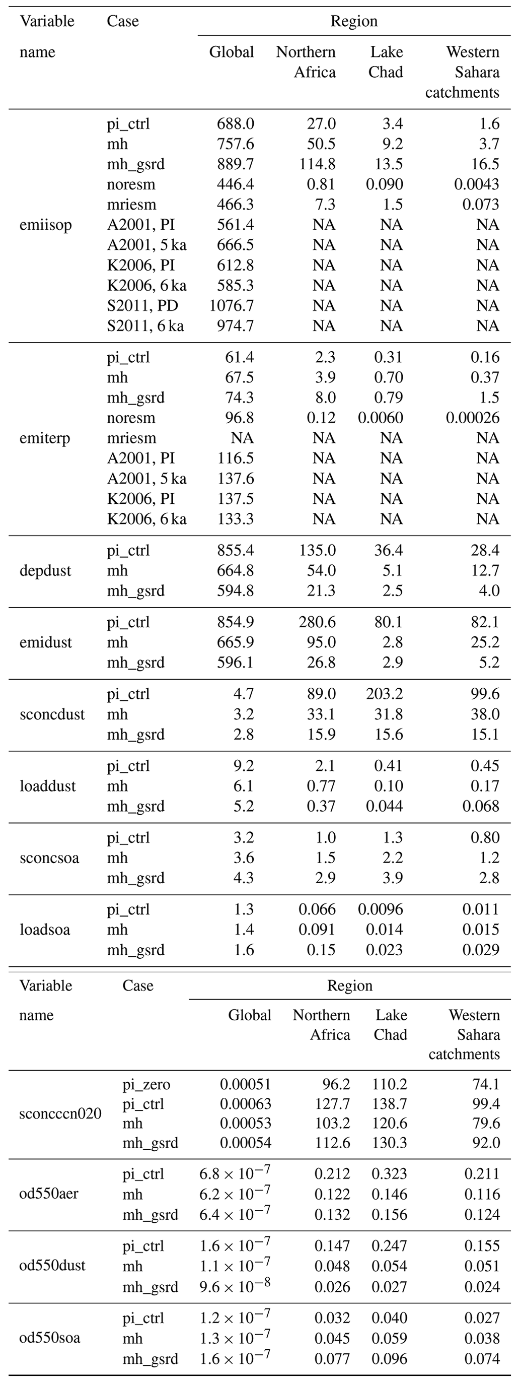
NA stands for not available.

Download XLSX

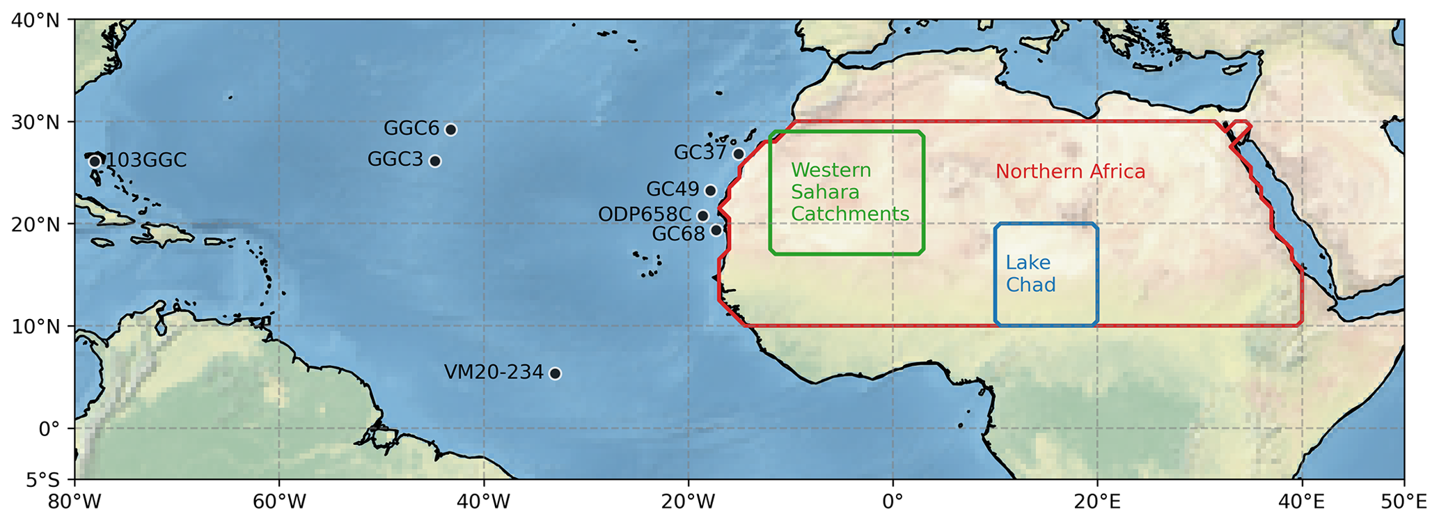
Figure 1The marine sediment sites and the regions. The exact location of the sites are listed in Table 3. The red line encloses the northern Africa (NA) region, which is defined as the African continent area within the region 20^∘ W to 40^∘ E and 10 to 30^∘ N. The blue box shows the Lake Chad (LC) region within 10–20^∘ E and 10–20^∘ N; the green box shows western Sahara catchments (WSC) region around the paleo-Lake Timbuktu area within 12^∘ W–3^∘ E and 17–29^∘ N. The map was plotted with the Python matplotlib package, and the data points were generated by the authors.

As a comparison, Arneth et al. (2008) summarized previous studies and showed that the estimated ranges of present-day global total annual emissions of isoprene and monoterpenes are from 412 Tg C a⁻¹ (467 Tg a⁻¹) to 601 Tg C a⁻¹ (681 Tg a⁻¹) and from 32 Tg C a⁻¹ (36 Tg a⁻¹) to 127 Tg C a⁻¹ (144 Tg a⁻¹), respectively. More recent studies, including the estimation of present-day global total annual BVOC emissions, present a varied picture. Hantson et al. (2017), for example, showed an estimate of 385 Tg C a⁻¹ (436 Tg a⁻¹) and 28.6 Tg C a⁻¹ (32.4 Tg a⁻¹) for isoprene and monoterpenes. Meanwhile, Cao et al. (2021) presented a range of 411 to 473 Tg C a⁻¹ (466 to 536 Tg a⁻¹) for isoprene emissions across all CMIP6 models. Sindelarova et al. (2022) modeled various BVOC species in different CAMS-GLOB-BIO inventory versions, showing an isoprene emission range of 299.1 to 440.5 Tg a⁻¹ and a monoterpene emission range of 63.2 to 82.7 Tg a⁻¹. In the unit conversion between Tg C and Tg, the molar masses of 12, 68 and 136 g mol⁻¹ are assigned to carbon, isoprene and monoterpenes.

2.4 Marine sediment record

The reconstructed dust mass deposition flux data at different marine sediment sites in North Atlantic were collected for the comparison with model results. The sediment sites are shown in Fig. 1 and Table 3 with GC37, GC49, GC68 and ODP658C along the northwest African coast, VM20-234, GGC3 and GGC6 in the remote Atlantic Ocean and 103GGC in the Bahamas. The ²³⁰Th (Thorium) normalization method was applied to calculate the dust fluxes at GC37, GC49, GC68 (McGee et al., 2013; Albani et al., 2015), ODP658C (Adkins et al., 2006), 103GGC and VM20-234 (Williams et al., 2016). The dust flux values at ODP658C were not given directly in the original references, so the terrigenous flux (F_terr) is calculated here with the original excess ²³⁰Th (Ex²³⁰Th) data according to the method in Adkins et al. (2006):

where β is the production rate of ²³⁰Th from ²³⁴U in the water column, equal to $\mathrm{2.63}\times {\mathrm{10}}^{-\mathrm{5}}$ dpm cm⁻³ ka⁻¹, and dpm represents disintegration per minute, which is a radioactive decay unit. Here z is the water depth of the sediment core location, which is 2263 m (deMenocal et al., 2000) and f_terr is the fraction of the terrigenous flux out of the total sediment flux, which is set to 45 % for MH period and 60 % for PI period (see Table 2 in deMenocal et al., 2000). It should be noted that the terrigenous flux, which includes both the fluvial/shelf-derived and the eolian terrigenous flux, typically exceeds the dust flux. Therefore, we only compared the eolian terrigenous flux with the modeled dust flux (McGee et al., 2013). Similarly, the dust flux values at GGC3 and GGC6 were also not provided directly in Middleton et al. (2018), so these values (F_dust) were calculated from the original data as

where [⁴He_terr] is the amount of terrigenous ⁴He (Helium) in the sediment in units of ncc g⁻¹ and ncc is equal to 10⁻⁹ cm³ at standard temperature and pressure. vsr is vertical sediment rain rate in units of g cm⁻² ka⁻¹; 5600 ncc g⁻¹ is applied to convert the ⁴He to ⁴He-based dust fluxes.

Table 3Reconstructed and modeled dust mass deposition fluxes (DMDF) at different sites. The references of reconstructed data are listed below the table. The estimated errors in reconstructed data are shown in the brackets if they are provided in the original references.

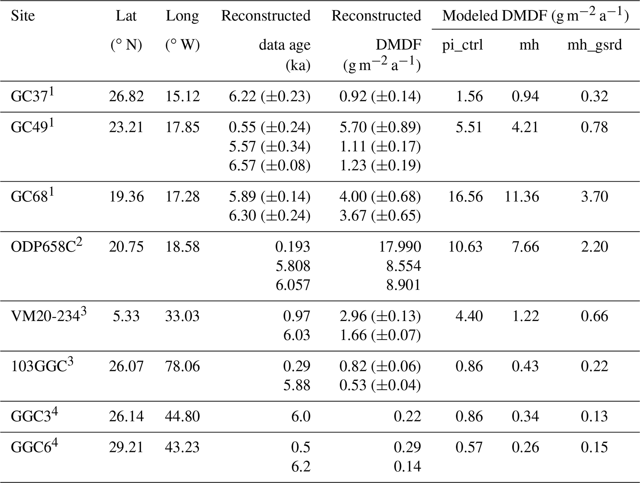
¹ McGee et al. (2013), Albani et al. (2015). ² deMenocal et al. (2000), Adkins et al. (2006). ³ Williams et al. (2016). ⁴ Middleton et al. (2018).

Download Print Version | Download XLSX

Since the reconstructed sample ages are not exactly at PI (0.1 ka, 1850 compared to 1950) or MH (in our model simulations assumed to be 6 ka), the data closest to 0.1 nd 6 ka were selected. For the PI period, only the data younger than 1 ka were selected. For example, for GC49, the data in 0.55 ka was selected for PI and the data in 5.57 ka and 6.57 were selected for the MH period. Moreover, the estimated errors of 1 standard deviation of age and dust flux data were also collected whenever they were available in the literature.

2.5 Study domains

In this study, we defined three regions for detailed analysis besides the globe scale. Firstly, northern Africa (NA) is defined as the African continent area within the region 20^∘ W to 40^∘ E and 10 to 30^∘ N. The other two regions are related to the paleo-waterbodies during MH where the dust emissions were reduced the most. One is the Lake Chad (LC) area within 10–20^∘ E and 10–20^∘ N and the other is the western Sahara catchments (WSC), centered around the paleo-Lake Timbuktu area within 12^∘ W–3^∘ E and 17–29^∘ N. The two paleo-lakes are selected because the Lake Chad has been suggested to have thrived between 11 and 5 ka (Armitage et al., 2015), and Lake Timbuktu is considered to have experienced a wet period between 9.5 and 3.5 ka (Drake et al., 2022). The regions are shown on the map in Fig. 1 and the regional-average and summed values in Table 2 refer to the regions defined here.

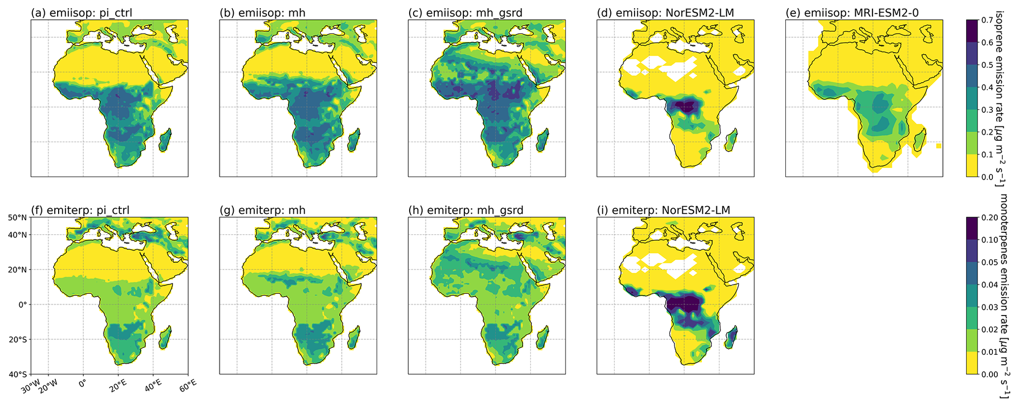
Figure 2Annual mean emission rates of isoprene (emiisop) over Africa from the simulation cases pi_ctrl (a), mh (b) and mh_gsrd (c), as well as the PMIP4 simulation results of NorESM2-LM (d) and MRI-ESM2-0 (e). The annual mean emission rates of monoterpenes (emiterp) are also shown for simulation cases pi_ctrl (f), mh (g) and mh_gsrd (h) and the simulation results of NorESM2-LM (i).

3.1 Surge in BVOC emissions

In the absence of available paleo-proxies to directly derive the BVOC emission data, we must rely on model simulations. Currently, the only available model results of BVOC emissions during MH from the PMIP4-CMIP6 midHolocene experiments come from NorESM2-LM and MRI-ESM2-0 simulations as mentioned above. Figure 2 shows the total annual emission rates of isoprene and monoterpenes from simulation cases pi_ctrl, mh and mh_gsrd in the present study, along with the results from NorESM2-LM and MRI-ESM2-0.

Due to the northward extension of vegetation cover over the NA region in the mh and mh_gsrd cases (elucidated in Lu et al., 2018), the emissions of both isoprene and monoterpenes increase compared to the pi_ctrl case (Fig. 2a–c and f–h). Notably, the BVOC emissions nearly cover the entire NA region in mh_gsrd (Fig. 2c and h). The total isoprene emissions over the NA region are 27.0, 50.5 and 114.8 Tg a⁻¹ in pi_ctrl, mh and mh_gsrd, respectively. Correspondingly, the monoterpene emission rate is 2.3, 3.9 and 8.0 Tg a⁻¹, respectively (Table 2). The relative increase in mh compared to pi_ctrl is 87 % for isoprene emissions and 70 % for monoterpene emissions, respectively. The mh_gsrd case, on the other hand, marks a more dramatic surge, with isoprene and monoterpene emissions increasing to 4.3 times and 3.5 times that of pi_ctrl, respectively.

Compared with the mh and mh_gsrd cases, the NorESM2-LM and MRI-ESM2-0 show lower isoprene emission rates over NA than the pi_ctrl case (Fig. 2a, d and e), which are 0.81 and 7.3 Tg a⁻¹, respectively. Moreover, the BVOC emissions in these two models are mostly centered over central Africa, encompassing the present-day Congolian rainforest (Fig. 2d, e and i). In contrast, in our cases pi_ctrl, mh and mh_gsrd, in which the vegetation cover was simulated by the vegetation dynamic model LPJ-GUESS, the BVOC emissions are more evenly distributed over central and southern Africa, and they remain substantial at the southern end of Africa, reaching 0.4 µg m⁻² s⁻¹ for isoprene emissions and 0.03 µg m⁻² s⁻¹ for monoterpene emissions.

Besides the PMIP4-CMIP6 midHolocene experiment results, several studies have also provided estimates of BVOC emissions during the MH, as mentioned in Sect. 2.3. Among them, only Adams et al. (2001) reported a rise in isoprene emissions during MH compared to PI or present-day levels, in which the global total annual emission rate of isoprene increased by 19 % and of monoterpenes by 18 %, given the reconstructed vegetation cover. Moreover, in Fig. 1a and d in Adams et al. (2001) we can see that the area with isoprene emission rates larger than 2 Tg M km⁻² a⁻¹ (about 0.06 µg m⁻² s⁻¹, here the unit in Fig. 1 in Adams et al. (2001) is Tg M ha⁻¹ a⁻¹, but this is a typo and the correct unit is Tg M km⁻² a⁻¹) moves northward over NA in 5 ka, and the area with emissions greater than 15 Tg M km⁻² a⁻¹ (about 0.48 µg m⁻² s⁻¹) increased in the Sahel region.

In this study, the total annual global emissions of isoprene and monoterpenes are 889.7 and 74.3 Tg a⁻¹ in the mh_gsrd case and 688.0 and 61.4 Tg a⁻¹ in the pi_ctrl case, respectively. These values align with the higher BVOC emissions during the MH similar with that in Adams et al. (2001). Conversely, Kaplan et al. (2006) noted lower BVOC emissions in 6 ka, with 585.3 Tg a⁻¹ for isoprene and 133.3 Tg a⁻¹ for monoterpenes compared to 612.8 and 137.5 Tg a⁻¹ during the PI period. They also specified that their vegetation simulations could not reproduce the northward shift of vegetation over Sahara region, likely due to their climate model (HC-UM, Hadley Centre Unified Model) unable to capture the interactive processes between land, atmosphere and ocean. Singarayer et al. (2011) also showed a decreasing trend of global isoprene emission rate from the PI period to the MH period. Moreover, to our knowledge, no recent studies have probed the BVOC emissions during the MH, despite Adams et al. (2001) proposing about 2 decades ago that such exploration could significantly enhance our understanding of past climate change.

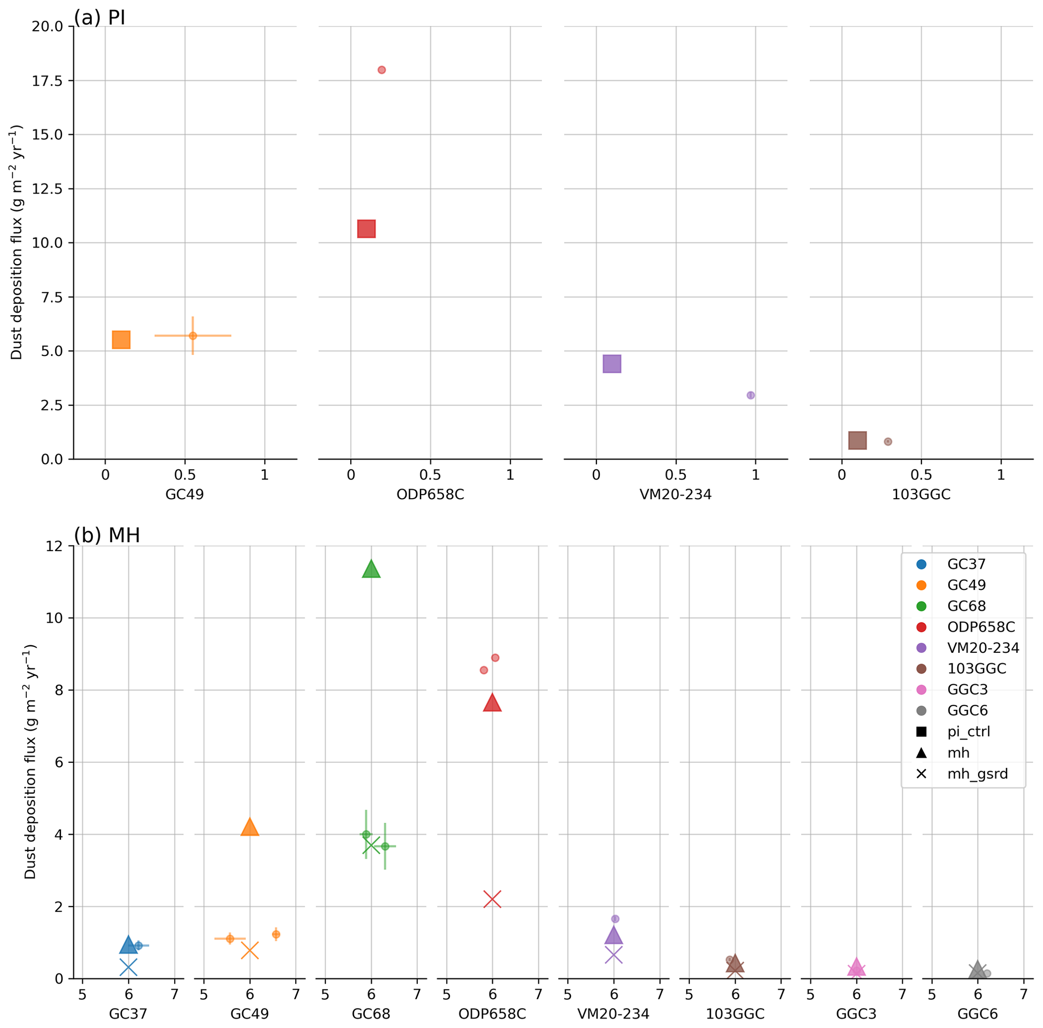
Figure 3Reconstructed (circles) and modeled (square for pi_ctrl, triangle for mh and cross for mh_gsrd) dust deposition fluxes during (a) PI and (b) MH periods. Different colors are set for different sediment sites which are shown in the legend. The x axis shows the age in units of ka. The error bars of dust fluxes are plotted for GC37, GC49, GC68, VM20-234 and 103GGC, and the age error bars are plotted for GC37, GC49 and GC68.

Download

3.2 Reduced dust emission

In order to verify our model simulation results, especially concerning new dust emission configurations, the modeled dust deposition fluxes were compared with the reconstructed data (Fig. 3). For the PI period, the model results agree well with the proxy data at GC49 and 103GGC (Fig. 3a). At ODP658C, the model result is only 59 % of the proxy data (Table 3). However, it should be noted that the dust flux at ODP658C may also include a fluvial/shelf-derived flux, estimated to be about 34 % of the actual dust flux as seen at the nearby site GC68 (see Fig. 3 in McGee et al., 2013). Consequently, the estimated actual dust flux at ODP658C during the PI is about 11.87 g m⁻² a⁻¹, closely aligning with our model result 10.63 g m⁻² a⁻¹. The model result at VM20-234 (Fig. 3a) should not be viewed as an overestimation but rather as consistent with the increasing trend of dust flux as we approach the PI era from 0.97 ka (see Fig. 2d in Williams et al., 2016).

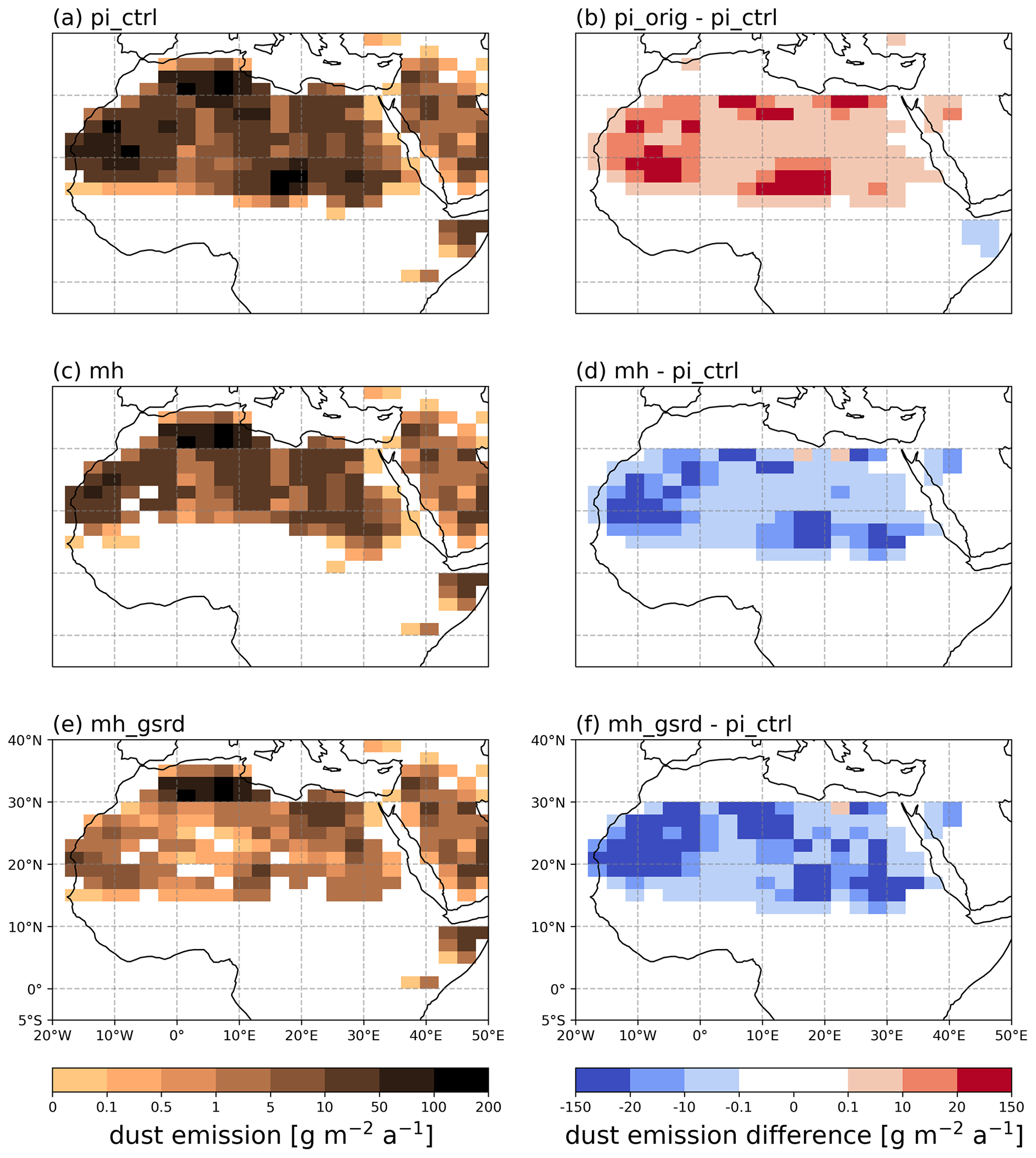
Figure 4Global annual dust emissions in units of g m⁻² a⁻¹ over central and northern Africa in the pi_ctrl (a), mh (c) and mh_gsrd (e) cases, as well as the dust emission differences between pi_orig and pi_ctrl (b), mh and pi_ctrl (d) and mh_gsrd and pi_ctrl (f), respectively.

During the MH period, the model results of both mh and mh_gsrd consistently reproduce the low dust fluxes at the remote sites, such as VM20-234, 103GGC, GGC3 and GGC6, despite underestimating the proxy data at VM20-234 (Fig. 3b). For the sites GC37, GC49 and GC68 along the northwest Africa coast, the model results in the mh case are consistent with the proxy data at GC37 but highly overestimate the values at GC49 and GC68 by about 3 to 4 times (Table 3). The mh_gsrd case, on the other hand, matches the proxy data at GC49 and GC68 but underestimates the value at GC37 (Fig. 3b). This indicates that the reduction in dust emissions due to the existence of waterbodies over the WSC region may be overestimated in the mh_gsrd simulation. As for ODP658C, as mentioned above, the reconstructed dust flux may exceed the actual value, and here the actual flux is estimated as $\mathrm{1}/\mathrm{2}$ to $\mathrm{1}/\mathrm{3}$ of the original value based on the observation at sites GC66 (19.944^∘ N, 17.860^∘ W) and GC68 (see Fig. 3 in McGee et al., 2013), yielding an estimate of about 2.91 to 4.36 g m⁻² a⁻¹. Therefore, based on the estimation, while the mh case drastically overestimates the proxy data, the mh_gsrd case underestimates the value but agrees better than mh (Table 3). The comparison results affirm that the new dust emission configuration in the model is able to predict the dust flux pattern during both PI and MH periods, as demonstrated by the pi_ctrl and mh_gsrd cases, respectively, across a substantial expanse stretching from the west Atlantic Ocean to the northwest coast of Africa.

Figure 4a shows that during the PI, the simulated dust emissions occur over the entire NA region, especially the Sahara region, reaching over 100 g m⁻² a⁻¹ in the regions such as LC, WSC and northern Algeria. However, during the MH the dust emissions decreased significantly, especially in the paleo-lake regions LC and WSC, where the total annual dust emissions are 2.9 and 5.2 Tg a⁻¹ in mh_gsrd and 2.8 and 25.2 Tg a⁻¹ in mh, respectively (Table 2).

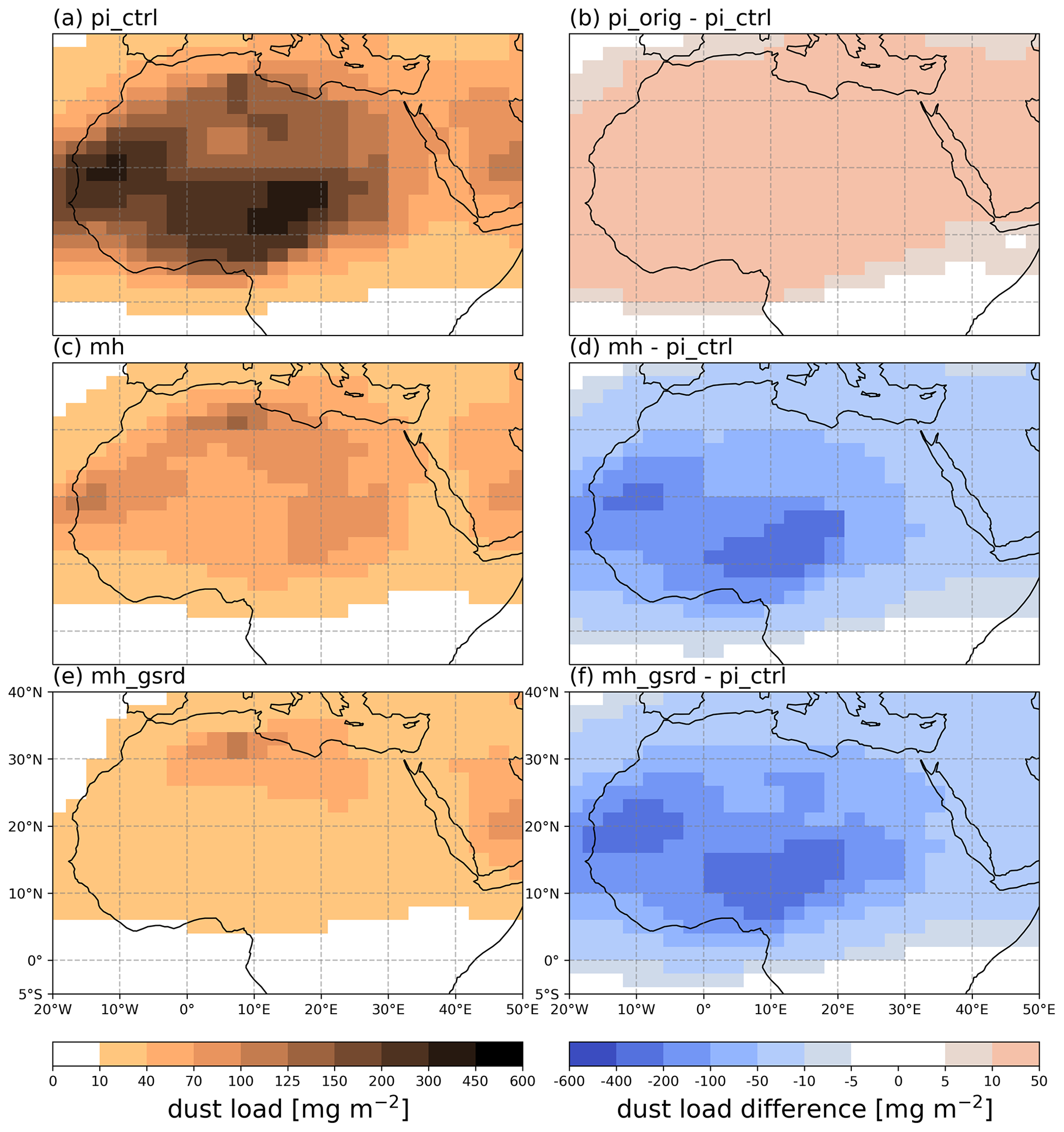
Figure 5Same as Fig. 4 but for dust load in units of mg m⁻².

The values of mh align closely in magnitude with the model results from Egerer et al. (2018) for 6 ka, but the annual dust emissions in the WSC region from the mh_gsrd case are only about 1 / 10 that over the similar western Sahara region in Egerer et al. (2018). This discrepancy could result from, besides the paleo-lake configuration, that we also set the FPAR values with reconstructed vegetation cover, which reduced the local dust emissions further. Later, when the paleo-lakes eventually dried out, the exposed slit material became vulnerable to surface wind, transforming the surrounding area into a major dust source (Tegen et al., 2002). This led to increased dust emissions during the PI period, resulting in 80.1 Tg a⁻¹ over the LC region and 82.1 Tg a⁻¹ over the WSC region under the pi_ctrl case (Table 2). Consequently, dust emissions are reduced by about 96 % and 94 % in the LC and WSC regions, respectively. Considering that the dust emissions in the default PI case pi_orig are even higher than in pi_ctrl (Fig. 4b), the relative reduction in dust emissions during the MH period compared to the PI period could be more pronounced.

The reduced dust emissions thus lead to a wide range of reduced surface dust concentration and dust load due to air-mass transport over NA during the MH period (Fig. 5). The most notable reduction in dust load in both the mh and mh_gsrd cases occurs over the LC and WSC regions, reflecting the dust emission differential pattern (Fig. 5d and f). The surface dust concentration closely correlated with dust load. When compared to pi_ctrl, the annual mean of these two variables over NA declined by 63 % in mh and 82 % in mh_gsrd, respectively. And interestingly, the relative reduction in dust load in the mh_gsrd case corresponds with the prescribed reduction percentage of dust mixing ratio below 150 hPa over NA in Pausata et al. (2016). This report provided the original MH climate forcing conditions for the dynamic vegetation simulations in Lu et al. (2018).

3.3 Increased SOA

In TM5-MP, isoprene and monoterpenes are the sole precursors of SOA formation (Bergman et al., 2022). Therefore, the modeled surface concentration of SOA mirrors the emission rates of isoprene and monoterpenes in individual cases (Fig. 6a, c and e).

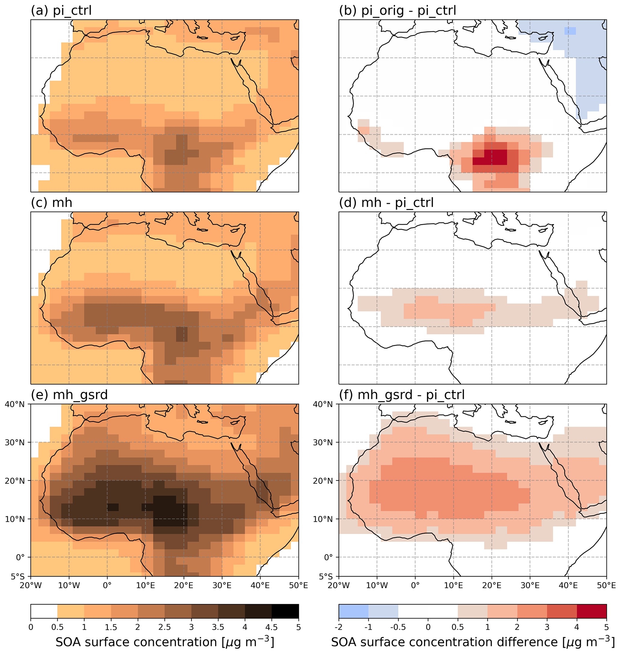
Figure 6Same as Fig. 4 but for SOA surface concentration in units of µg m⁻³.

In the pi_ctrl case, the peak SOA surface concentration appears in central Africa along the longitude 20^∘ E from around 0 to 10^∘ N, with the highest values exceeding 2.5 µg m⁻³ (Fig. 6a). In the mh case, SOA surface concentration increases due to higher BVOC emissions over the Sahel region with the highest recorded values exceeding 3.0 µg m⁻³ (Fig. 6c). Moreover, the northernmost region of maximum concentration extends further in this case compared to pi_ctrl, but it is primarily confined to a narrow belt between 10 and 20^∘ N, reflecting the less northward extension of BVOC emissions. Here the average relative increase in SOA surface concentration over the NA region is 50 % compared to pi_ctrl (Fig. 6d).

While in the mh_gsrd case, as the vegetation covers nearly the whole of Africa, especially the NA region compared to the other two cases, the SOA surface concentration is higher than 4.5 µg m⁻³ across western to central Africa (Fig. 6e). The significantly increased BVOC emissions due to northward extension of vegetation cover result in a more than 1 µg m⁻³ greater SOA surface concentration over nearly the entire NA region in mh_gsrd compared to pi_ctrl. The difference increases to over 2 µg m⁻³ across the western and central areas, resulting in a value 2.9 times greater than that in the pi_ctrl case over the NA region (Fig. 6f). Figure 6b shows that SOA surface concentration is lower in central Africa in pi_ctrl compared to original PI simulation case pi_orig. This indicates that over this area, the simulated SOA concentration during the MH period is lower than that in the pi_orig case due to lower vegetation cover.

3.4 Impact on size distributions and CCN

In order to estimate the potential impact of the increased SOA formation over NA region on cloud properties, we examined the CCN surface concentrations at supersaturations of 0.2 % (CCN0.2) (Fig. 7), which are roughly related to the number concentrations of particles larger than 100 to 200 nm (Jokinen et al., 2015). Within this size range, the CCN0.2 concentration is mainly determined by particles in the soluble accumulation (ACS) mode and soluble coarse (COS) mode (Figs. S3 and S4). Nevertheless, during the PI period, anthropogenic primary aerosol emissions from Europe enhanced the particle number concentration in ACS mode and consequently the CCN0.2 concentration (Fig. 7a and b), exceeding the impact of land cover change during the MH. Therefore, we conducted another simulation pi_zero which is the same as pi_ctrl but without any anthropogenic emissions. Compared to pi_zero, the average CCN0.2 surface concentration over NA in mh and mh_gsrd increased by about 7 % and 17 %, respectively.

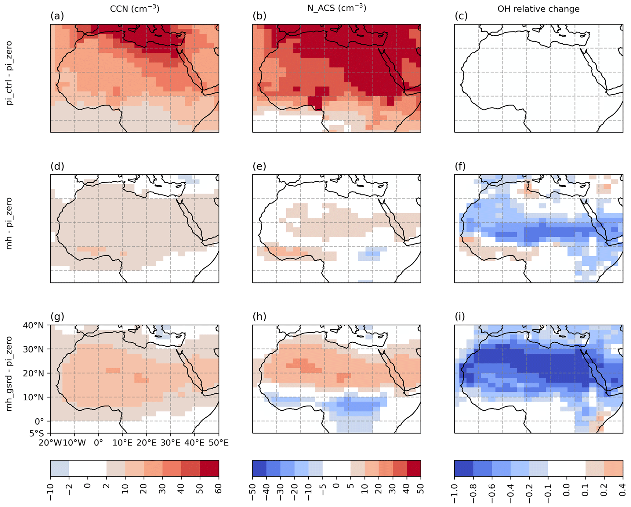
Figure 7The difference in (a) CCN at supersaturation of 0.2 % in units of cm⁻³, (b) number concentration of particles in the soluble accumulation mode (N_ACS) in units of cm⁻³ between pi_ctrl and pi_zero. (c) The relative change in OH surface number concentration in pi_ctrl compared to pi_zero. The same for (d, g) CCN, (e, h) N_ACS and (f, i) OH relative change but between mh and pi_zero, mh_gsrd and pi_zero, respectively.

The reduced dust emissions during the MH period decreased the mass concentration of COS mode over the NA region, but the number concentration was unaffected (Figs. S3 and S4). Concurrently, over the same region, the number concentration of ACS mode increased (Fig. 7e and h) due to the enhanced SOA concentration, which exceeded the impact of decreased sulfate concentration (Figs. S3 and S4), leading to increased CCN0.2 concentration (Fig. 7d and g). However, the hygroscopicity parameter of SOA is only 0.1 while for sulfate it is 0.6, so the CCN0.2 number concentration only increased by less than 10 and 20 cm⁻³ over the NA region in mh and mh_gsrd, respectively. It should be noted that the enhanced BVOC emissions not only increased SOA concentration but also consumed more OH (hydroxyl radical) via the oxidation reactions. Figure 7f and i show that the OH number concentration over the NA region in mh and mh_gsrd decreases more than 20 % and 60 % compared to the pi_zero case, respectively. This leads to reduced gas-phase sulfuric acid concentration which is produced mainly via the reaction between SO₂ (sulfur dioxide) and OH, and finally leads to lower sulfate concentration.

Figure 7e and h show a decrease in the ACS mode in central Africa in the mh and mh_gsrd cases, yet the CCN0.2 number concentration still shows positive change. The reduction in the number concentration of the ACS mode is mainly attributed to the decreased BC (black carbon) and POM (primary organic matter) (Figs. S3 and S4), which have hygroscopicity parameters of 0 and 0.1, respectively. Therefore, although the number concentration of ACS mode decreases, the average hygroscopicity of the particles could still increase due to the significant enhancement of SOA concentration over this region. Moreover, the average diameter of the ACS mode may not be affected due to the counteraction between the increased SOA concentration and the decreased concentrations of BC and POM.

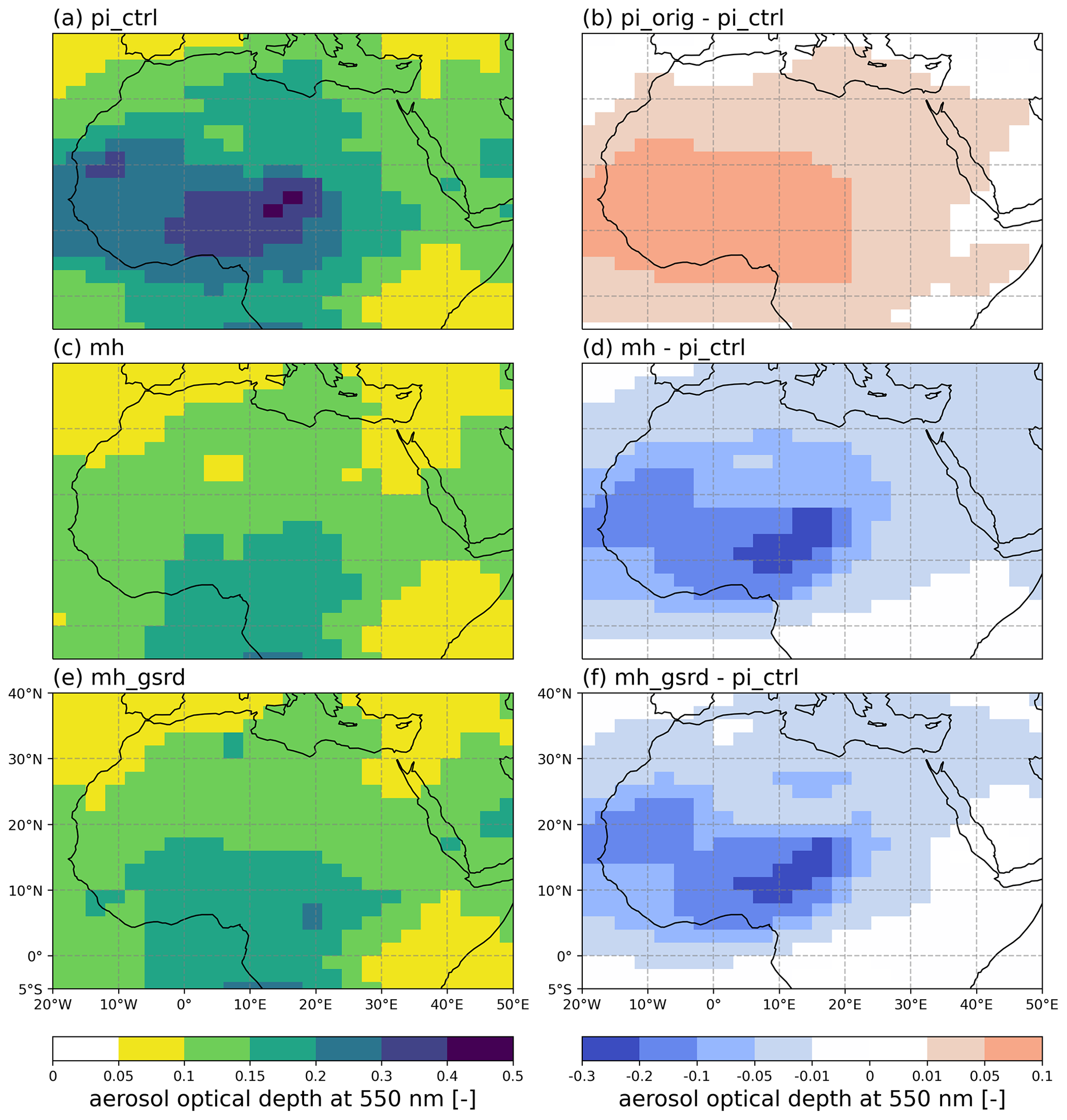
Figure 8Same as Fig. 4 but for aerosol optical depth at 550 nm.

In general, the enhanced BVOC emissions due to vegetation cover change are able to affect the cloud properties (e.g., reflectivity, lifetime and precipitation properties) via increasing CCN concentrations over the NA region, which needs to be kept in mind in future studies. Moreover, because of the complex consequences originating from the changed BVOC emissions as mentioned above, one should be careful when analyzing the aerosol–cloud interactions.

3.5 Reduction in AOD

During the PI period, the aerosol optical depth at 550 nm (AOD550) over NA is dominantly affected by the dust load (Figs. 8a and 5a). The dust emission source areas surrounding LC region show the highest aerosol optical depth, exceeding 0.3. During the MH, these areas along with their downwind locations show the largest reduction in AOD550 at around −0.3 in both mh and mh_gsrd cases (Fig. 8d and f). Both cases demonstrate similar patterns of AOD550 variation over NA. Interestingly, although the dust load in mh_gsrd is about 51.9 % lower than that in mh over NA region, the AOD550 in mh_gsrd remains 0.01 higher, which is about 8.2 % increase compared to that in mh. This suggests that the AOD550 increase due to the increasing of SOA surpasses the AOD550 reduction due to the decrease in dust. For example, in the mh case, the AOD550 over the NA region is split between 0.048 (51.6 %) for dust and 0.045 (48.4 %) for SOA, while in the mh_gsrd case, the values shift to 0.026 (25.2 %) and 0.077 (74.8 %), respectively. Given that mh_gsrd is the more realistic case, neglecting the AOD550 change due to the increased SOA over NA during the MH would result in underestimating the AOD550 by 0.045 (i.e., 0.077 minus 0.032). This accounts for about 21.2 % of AOD550 in pi_ctrl case. Our result of AOD550 for dust over the NA region in mh_gsrd is 0.026, which aligns with the simulation result of “MH control” (0.02 over Sahara) as presented in Thompson et al. (2019).