the Creative Commons Attribution 4.0 License.
the Creative Commons Attribution 4.0 License.
 | 21 Jul 2023
The effect of the Pliocene temperature pattern on silicate weathering and Pliocene–Pleistocene cooling
John C. H. Chiang
Nicholas L. Swanson-Hysell
The warmer early Pliocene climate featured changes to global sea surface temperature (SST) patterns, namely a reduction in the Equator–pole gradient and the east–west SST gradient in the tropical Pacific, the so-called “permanent El Niño”. Here we investigate the consequences of the SST changes to silicate weathering and thus to atmospheric CO2 on geological timescales. Different SST patterns than today imply regional modifications of the hydrological cycle that directly affect continental silicate weathering in particular over tropical “hotspots” of weathering, such as the Maritime Continent, thus leading to a “weatherability pattern effect”. We explore the impact of Pliocene-like SST changes on weathering using climate model and silicate weathering model simulations, and we deduce CO2 and temperature at carbon cycle equilibrium between solid Earth degassing and silicate weathering. In general, we find large regional increases and decreases in weathering fluxes, and the net effect depends on the extent to which they cancel. Permanent El Niño conditions lead to a small amplification of warming relative to the present day by 0.4 ∘C, suggesting that the demise of the permanent El Niño could have had a small amplifying effect on cooling from the early Pliocene into the Pleistocene. For the reduced Equator–pole gradient, the weathering increases and decreases largely cancel, leading to no detectable difference in global temperature at carbon cycle equilibrium. A robust SST reconstruction of the Pliocene is needed for a quantitative evaluation of the weatherability pattern effect.


Evidence has been accumulating that east–west (zonal) gradients of sea surface temperature (SST) and thermocline depth in the tropical Pacific were reduced during the warm early Pliocene (4.5–3 Ma) with respect to modern conditions (e.g., Cannariato and Ravelo, 1997; Ravelo, 2004; Wara et al., 2005; Fedorov et al., 2013). These features, resembling modern El Niño events, have led to the idea of a “permanent El Niño” climatic state during the Pliocene epoch, also named “El Padre” (Shukla et al., 2009). Paleoclimate proxy data also support the fact that the average Equator–pole (meridional) temperature gradient was reduced during the warm early Pliocene (Brierley et al., 2009; Brierley and Fedorov, 2010; Fedorov et al., 2013).
The transition between early Pliocene to modern climate conditions is thought to be linked to global cooling from the Pliocene (5.3 to 2.6 Ma) into the Pleistocene (2.6 to 0.01 Ma), as both a cause and a consequence. This global cooling since the Pliocene has occurred, while there is little evidence of significant change in CO2 outgassing (e.g., Herbert et al., 2022), suggesting another trigger. Molnar and Cronin (2015) argued that the onset of a modern tropical Pacific zonal SST gradient (due to the larger cooling of the eastern tropical Pacific) may have permitted the inception of the Laurentide ice sheet, promoting global cooling. In this hypothesis, teleconnection altered the atmospheric circulation over North America, thereby enabling accumulation of perennial snow in winter in northern North America. The authors developed the hypothesis that vigorous modern Pacific Walker circulation was caused by the restriction of the Indonesian seaway and the increased land area of emerged islands in the Maritime Continent, both due to tectonic processes associated with arc–continent collision. The Walker circulation is an east–west atmospheric overturning circulation near the Equator that interacts with an oceanic counterpart, setting up a zonal SST gradient across the ocean basin. On the other hand, Fedorov et al. (2006) proposed a feedback loop whereby shoaling of the thermocline with cooling climate activates the Bjerknes feedback – the amplification of the cooling of the eastern boundary of a equatorial basin through upwelling of cold water due to easterly winds. This feedback promotes easterlies, thus invigorating the Walker circulation and further enhancing climate cooling through cloud albedo and ice albedo feedback. The zonal tropical Pacific SST gradient has also been shown to be linked to the global meridional temperature gradient (Fedorov et al., 2015). Therefore, all the following elements, i.e., strengthening zonal and meridional gradients, intensification of the El Niño–Southern Oscillation (ENSO), the onset of a mean climate state closer to La Niña and global cooling, would be connected processes.
One element that has been largely overlooked in these considerations about regional climate changes is their effect on silicate weathering and the silicate weathering feedback. The so-called silicate weathering paleothermostat (Walker et al., 1981) is the hypothesis that long-term climate is controlled by the balance between deep Earth degassing of CO2 and its consumption by continental silicate weathering as well as associated oceanic carbonate precipitation (the Urey reaction, Urey, 1952). Weathering reactions are enhanced by a warmer climate, which introduces a negative feedback: atmospheric CO2 is stabilized at the level where its consumption balances its degassing (Walker et al., 1981; Berner et al., 1983). Continental runoff rate is a key factor controlling silicate weathering rate (Gaillardet et al., 1999; Dessert et al., 2003; Oliva et al., 2003; Maher and Chamberlain, 2014). The very existence of the silicate weathering paleothermostat relies to a large extent on the fact that runoff rates, on average, increase with rising CO2 and associated global warming (Kukla et al., 2022). Hence, processes that affect the distribution of continental runoff, even without direct effects on global temperature, have the potential to change the efficiency of silicate weathering and therefore equilibrium atmospheric CO2 level as well as global temperature. This phenomenon is analogous to the so-called “pattern effect” (Langenbrunner, 2020) in the Earth's temperature climate sensitivity to atmospheric CO2. As with climate sensitivity, SST patterns may have significant effects on the efficiency of silicate weathering – hereafter called “weatherability” – because they affect atmospheric convection, precipitation and runoff.
In that regard, reducing meridional or zonal SST gradients (with respect to modern climate) may decrease global weatherability by shifting rainfall away from tropical land masses. In the case of meridional gradient, Burls and Fedorov (2017) suggested a reduced equatorward moisture transport by the Hadley circulation with a flatter SST gradient. This feature can be summarized by “wet gets drier, dry gets wetter” (Burls and Fedorov, 2017). In the case of zonal gradients, a weaker Pacific gradient should lead to reduced Pacific Walker circulation, which is responsible for intense precipitation over the Maritime Continent in the modern climate. Indeed, El Niño events, wherein the Pacific Walker circulation collapses, lead to a drastic decrease in continental runoff on the Maritime Continent, as well as most of South America near the Equator (see Fig. 1 showing the climatology of precipitation and runoff for El Niño years). On average, runoff is reduced by ∼3 % on land during El Niño years. The key element here is that some tropical areas that are drier in El Niño years are known hotspots of silicate weathering – mainly the Southeast Asian islands known as the Maritime Continent (Figs. 1 and 2a). Another contribution to changes in silicate weathering should be expected from the Himalaya and the portion of the Andes north of the Equator, which also experience decreases in runoff during El Niño years.
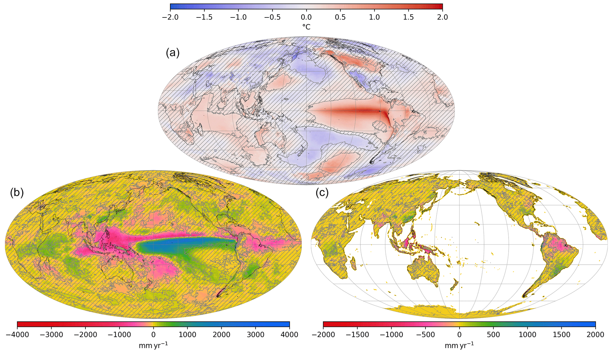
Figure 1Differences in climatology associated with El Niño years: the average of selected El Niño years minus the average of years selected neither as El Niño nor as La Niña. Each “year” considered here is from May to the following April. Data are from ERA5 reanalysis. See Methods, Sect. 2.2 and Appendix A for details. (a) 2 m temperature, (b) total precipitation and (c) continental runoff. In each panel, non-significant differences are hatched (p value of Welch's t test > 0.1, see Appendix C). The maps are Mollweide projections with graticules plotted every 30∘ of longitude and every 20∘ of latitude (both starting from 0∘). Note that it is significantly drier over the Southeast Asian islands in El Niño years with more precipitation falling over the tropical Pacific Ocean than over land.
The above text and associated hypothesis can be summarized as follows: with weaker meridional and zonal temperature gradients, the decrease in runoff over land, specifically on tropical weathering hotspots, would lead to reduced weatherability and, as a result, higher CO2 levels contributing to the warmer Pliocene climate. If we further assume that a colder climate favors stronger meridional and zonal gradients, the overall process of cooling would act as a positive feedback loop whereby increased cooling leads to increased precipitation on key land masses, which would lead to enhanced weatherability and increased cooling. This process has the potential to have amplified climate cooling from the warm early Pliocene into the Pleistocene.
In this contribution, we investigate the potential effect of meridional and zonal gradients on global climate through the silicate weathering feedback, without seeking to determine the cause of these regional climate features. We first provide an estimation of the silicate weathering anomaly using the climate fields from ERA5 reanalysis 1979–2020 (Muñoz Sabater, 2019; Hersbach et al., 2019), with the assumption that the average climate of El Niño events can be used as a proxy for Pliocene permanent El Niño. This method enables a qualitative assessment of whether the effect of a permanent El Niño state on global chemical weathering would generate a warmer or colder global climate (because of a decrease or increase in chemical weathering, respectively). However, one cannot quantitatively estimate this warming or cooling because the climate reanalysis only exists at the current CO2 level. Yet, any disturbance in the efficiency of silicate weathering – that is, an increase or decrease in silicate weathering flux at the current CO2 level – will change CO2 until the balance between CO2 degassing and its consumption by silicate weathering is restored. On the million-year timescale of the Pliocene to the modern, it is this equilibrium CO2 level that matters for climate evolution. Furthermore, it is possible that the average of El Niño years is not a perfect analog of a permanent El Niño because of the transient nature of those events and the fact that they are not bound to radiative balance, as is a long-term equilibrium climate state.
For these two reasons, we designed numerical climate experiments aimed at exploring Pliocene climate features with a climate model, focusing on the meridional and zonal tropical SST gradient. Doing so, we provide an initial quantitative estimation of the role of a weatherability pattern effect in climate evolution since the warm early Pliocene through the silicate weathering feedback.
2.1 Silicate weathering model
We use the silicate weathering model published in Park et al. (2020), hereafter referred to as GEOCLIM. This model represents the steady-state vertical profile of primary silicate mineral abundance in a regolith – the interface between unweathered bedrock and land surface. Minerals are progressively weathered until they are removed from the regolith through physical erosion of the surface. Hence, weathering profiles show a continuous depletion of primary minerals from bedrock to the surface. The vertically integrated weathering rate depends on the rate of physical erosion (which leads to upward advection of primary minerals), the efficiency of weathering chemical reactions (that depend on runoff and temperature) and the residence time of minerals in the regolith (that is also controlled by the physical erosion rate). The derivation of this model was carried out by Gabet and Mudd (2009) and West (2012), who parameterized the climatic control of weathering reactions (through temperature and runoff). The erosion rate is computed as a power law of topographic slope and runoff rate (Maffre et al., 2018; Park et al., 2020).
The value of interest computed by the weathering model is the amount of dissolved Ca and Mg released by weathering of silicate minerals (integrated over the regolith profile). This flux corresponds to long-term CO2 consumption in the geological carbon cycle through the eventual precipitation of marine carbonates. The weathering model is applied to every point of the continental mesh grid at the resolution of the climate fields used (see following sections). At each point, computation of the estimated weathering rate is done for five lithological classes of silicates (as in Park et al., 2020) that are simplified from the global lithological map of Hartmann and Moosdorf (2012). The slope field was derived from the elevation dataset of the Shuttle Radar Topography Mission (Farr et al., 2007) at 30 arcsec resolution. Both the lithological classes and the slope were interpolated on the desired mesh grids.
The model parameters are taken from Park et al. (2020), who provided an ensemble of 573 “best-fit” unique parameter combinations resulting from a comparison of model results to modern chemical weathering fluxes across watersheds. As in Park et al. (2020), the weathering model is run with all those unique parameter combinations. We present, for each model run, the ensemble of results (e.g., the ensemble of the global weathering flux). This approach allows us to quantify the uncertainties arising from the weathering parameters.
The silicate weathering model does not explicitly represent the role of vegetation as a weathering agent. Yet, because it is calibrated with data from natural systems, the parameters incorporate some of the vegetation effects embedded in the data. For instance, the values of parameters determining the sensitivity to the runoff (kd and kw) are influenced by the correlation between water availability and the presence of vegetation.
2.2 Climate reanalysis and selection of El Niño and La Niña years
The reanalysis climate fields used in this study are from ERA5-land 1981–2019 (Muñoz Sabater, 2019) for continental runoff and ERA5 1979–2020 (Hersbach et al., 2019) for 2 m temperature and SST. The monthly averaged fields at the native resolution (0.1∘ for ERA5-Land and 0.25∘ for ERA5) were interpolated on a longitude–latitude grid of 0.5∘ resolution.
To determine the climatology associated with El Niño and La Niña years, we generated an interannual index of ENSO and then used it to create selections of El Niño years, La Niña years, and neither El Niño nor La Niña years. The details of the calculation of this ENSO index can be found in Appendix A. Based on this index, we selected the years 1982, 1987, 1991, 1997, 2009 and 2015 as El Niño years and the years 1984, 1988, 1999, 2007 and 2010 as La Niña years (in each case, from May to April of the next calendar year).
2.3 Climate model
For the climate numerical experiments, we used the Community Earth System Model (CESM) version 1.2.2.1. The experiments were conducted using the components CAM4 (Community Atmospheric Mode version 4) for the atmospheric dynamics, CLM4.0-CN (Community Land Model version 4.0, Carbon–Nitrogen), RTM (River Transport Model) river runoff component, CICE (Community Ice CodE) prognostic sea ice, and, for the oceanic component, either fixed-SST DOCN (Data Ocean), slab ocean DOCN, or full ocean model POP2 (Parallel Ocean Program version 2). The slab ocean approximates a well-mixed ocean mixed layer with a fixed depth set to the annual mean; an ocean heat transport convergence (i.e., the Q flux) from a CESM1 pre-industrial fully coupled run is prescribed at each ocean grid point to achieve a simulated sea surface temperature close to the pre-industrial. The grids used are a regular (latitude × longitude) for atmosphere and land modules, a regular 0.5∘ for runoff routing, and a ∼1∘ “displaced” grid with Greenland pole (0.9×1.25_gx1v6) for the ocean models (both slab and full) and sea ice modules.
All experiments were conducted with permanent 1850 (pre-industrial) boundary conditions, with the exception of the few modifications discussed later in the article, which are atmospheric CO2 concentration, slab ocean Q flux and cloud albedo. Experiments were run for 40 years for the fixed-SST cases, 50 years for the slab ocean cases and 230 years (170 years for the control) for the coupled ocean–atmosphere cases. All experiments were initiated with a “cold start” (internally generated initial condition, corresponding to a pre-industrial climate). In all cases, the last 30 years of the model runs were used to compute the climatology average. See Table B1 and Appendix B for more information about the specific features of the climate simulations conducted here.
2.4 Geographic division of silicate weathering
To quantify the contributions of the different regions of Earth to the changes in silicate weathering flux due to perturbations of climate fields, we used the geographic division shown in Fig. 2a. This division is meant to isolate known weathering hotspots (e.g., Maritime Continent and East African Rift), major mountain ranges and, for the remaining regions, tropics versus subtropics. The boundaries of these regions are somewhat arbitrary, especially for the mountain ranges, and their naming should be considered a simplification of the broader regions. For instance, “Himalaya” refers to the merging of the Himalayan range and its extension over the Longmen Shan, Southeast Asia, the Tibetan plateau and the Tian Shan. Despite the subjectivity of those boundaries, these divisions give a sense of the different response of individual regions that are useful for summarizing results.
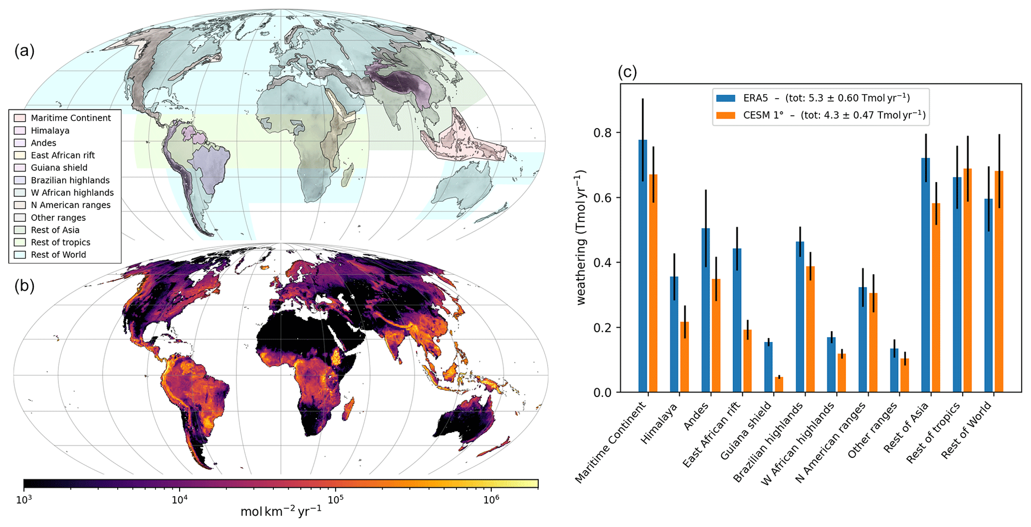
Figure 2(a) Map of the geographic division used to summarize results in this study (colored semi-transparent shades) superimposed on land topography. (b) Average chemical weathering rates (Ca and Mg from silicate minerals) over the parameter combinations (i.e., the weathering model is run for each of the 573 selected parameter combinations, and the 573 weathering fields are then averaged). Weathering is computed using climate fields from ERA5 reanalysis (climatology average 1981–2019) at 0.5∘ resolution. (c) Bar plot of chemical weathering fluxes integrated over the geographic regions (panel a) using ERA5 climate fields, as for panel (b) (blue bars), or using climate fields from the CESM1.2 climate model pre-industrial control simulation, with a slab ocean model, as performed in this study (average of the last 30 years of simulations; orange bars). The main colored bars denote the average weathering flux of the 573 parameterizations, whereas the black error bars denote the standard deviation over those parameterizations. The total (summed) weathering flux is indicated in the legend box, giving both the average and associated standard deviation resulting from the different weathering model parameterizations. The map projections and graticules (panels a and b) are similar to Fig. 1.
3.1 Weathering rates using ERA5 reanalysis
3.1.1 Control simulation
We first run the weathering model using ERA5 reanalysis of climate fields (1981–2019 climatology average) as a control simulation. The resulting weathering rates (averaged over the selected parameterizations) are presented on a map in Fig. 2b. The total CO2 consumption by weathering is 5.3 Tmol yr−1. This control weathering field is very similar to the one published in Park et al. (2020, Fig. S5 of their contribution), who used the same model, parameter combinations and slope fields, but different climate fields (CRU TS v.4.03 for the temperature, Harris et al., 2014, and UNH/GRDC Composite Runoff Fields V1.0, Fekete et al., 1999).
The contribution of the different regions of Earth to this control weathering flux is shown in Fig. 2c (blue bars). The weathering flux from the Maritime Continent is about 11 % of the total flux, which is consistent with previous estimates (e.g., Molnar and Cronin, 2015). The main mountain belts (broader Himalaya, the Andes, and North and Central American ranges, including the Rocky Mountains) together contribute ∼22 % of the total. Another significant weathering contributor is the East African Rift (∼8 % of the total) owing to relatively high runoff rates, the substantial amount mafic silicate rock exposed and the relatively steep topography that fosters physical erosion – and hence, elevated chemical weathering fluxes. Taiwan and New Zealand, which are known hotspots of physical erosion rates, do not contribute significantly to the total chemical weathering flux because of the limited areal extent of their orogens.
3.1.2 Climatologies of El Niño and La Niña years
We then recompute the weathering rates with the same dataset, but keeping only the years of the climate time series identified as “El Niño” or “La Niña” (average of May to April, see Methods, Sect. 2.2). The anomaly of Earth-integrated weathering flux is Gmol yr−1 for El Niño years and Gmol yr−1 for La Niña (with ± denoting the standard deviation of the weathering anomaly over the selected parameterizations). These calculations assume that these climatologies are imposed over a long timescale such that the chemical weathering profiles adjust to result in these fluxes. Assuming that CO2 degassing is constant, these weathering anomalies would in reality be compensated for by global warming or cooling so that the net silicate weathering flux anomaly is zero. If we extrapolate from the silicate weathering feedback computed with CESM climate simulations, indicating a global weathering flux increase of ∼0.4 Tmol yr−1 ∘C−1 of global warming by CO2 (Fig. 8b, solid black curve), the weathering anomalies should then be compensated for by global mean temperature anomalies of +0.23 ∘C for long-term El Niño conditions and −0.35 ∘C for long-term La Niña conditions. These relatively small values of weathering anomaly (1.7 % and 2.6 % of the total control flux, respectively) are the consequences of a local increase and decrease in weathering rates that compensate for each other (Fig. 3). Nevertheless, the differences from 0 are robust among all the selected parameterizations (the absolute anomaly of weathering flux is ∼4 times larger than the standard deviation due to the parameter uncertainties) and approximately symmetrical between El Niño and La Niña conditions. These results support our hypothesis of climate cooling caused by the progressive onset of La Niña-like mean climatic conditions, though the magnitude of this cooling may not have been substantial.
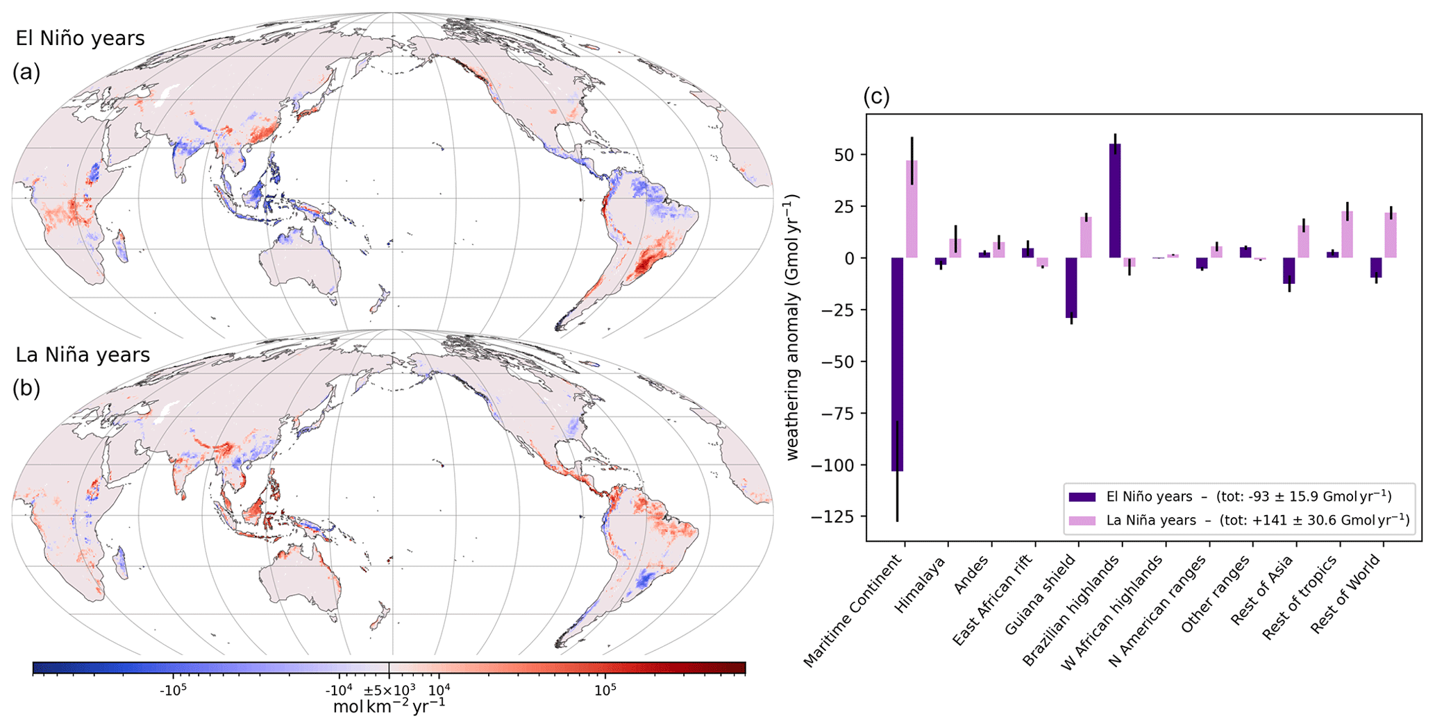
Figure 3(a, b) Anomaly of modeled weathering rate with respect to control weathering (i.e., the field shown in Fig. 2b) for climatology in El Niño years (a) and La Niña years (b). The weathering rate is averaged over the parameter combinations (as in Fig. 2b). The color bar scale is a “symmetric logarithm”, and any value lower than 5×10³ mol km−2 yr−1 (in absolute value) is approximated as 0. Map projection and graticules are as in Fig. 1. (c) Bar plot of the anomaly of weathering flux integrated over the geographic regions shown in Fig. 2a with respect to ERA5 control weathering (blue bars in Fig. 2c) for climatology in El Niño or La Niña years. The average (main colored bars) and standard deviation (error bars) refer to the parameterizations, as in Fig. 2c. There are many regional changes of note as discussed in the text. For example, there is enhanced weathering over the Maritime Continent during La Niña years relative to El Niño years. The change in weathering rate is most dramatic over the Maritime Continent due to increased precipitation over land during La Niña years compared to being over the Pacific Ocean during El Niño years.
Local weathering anomalies are largely driven by changes in runoff rates. Many regions display dipolar patterns under El Niño conditions (Fig. 3a). For example, weathering fluxes increase on the Ethiopian Traps associated with El Niño conditions but decrease on the southern part of the East African Rift. They increase in the Andes near the Equator but decrease in the northernmost part of the range, and they decrease on the central Himalaya but increase in the western part. Hence, the anomaly of weathering flux integrated over those regions is close to zero (Fig. 3c). Most of the negative anomaly of El Niño weathering comes from the Maritime Continent. The weathering integrated over this region is almost equal to the total anomaly (Fig. 3c, purple bars). This result highlights the key role this area has potentially played in cooling Earth's climate over the last few million years. The signal from the Maritime Continent is expanded by a weathering decrease on the Deccan Traps and the Guiana highlands associated with El Niño conditions and partially offset by an increase on the Brazilian highlands (Fig. 3).
It is interesting to note that although the sign of weathering anomalies under La Niña conditions is the opposite of the ones under El Niño conditions nearly everywhere, the magnitude of those anomalies is not perfectly symmetrical (Fig. 3c).
3.2 Exploring the consequences of Pliocene SST
We wish to take a step further here and investigate the consequence of Pliocene-like gradients of SST for silicate weathering and equilibrium temperature (i.e., the global mean temperature for which silicate weathering balances degassing). We rely on the work of Fedorov et al. (2015), demonstrating that the tropical zonal gradient of SST is linked to the meridional gradient of SST. This result indicates that Pliocene permanent El Niño could be a consequence of a weakened meridional gradient. Drawing from their work, we designed climate simulations aimed at mimicking Pliocene SST, following the method of Burls and Fedorov (2014).
The climate simulations presented in Burls and Fedorov (2014, 2017) and Fedorov et al. (2015) cannot be directly used because the simulations at resolution were only conducted at pre-industrial CO2. However, estimating carbon cycle equilibrium with GEOCLIM necessitates climate simulations at several CO2 levels. This cannot be done with fixed-SST simulations (such as from Fedorov et al., 2015) because it will miss the warming of the ocean surface with rising CO2. On the other hand, changing atmospheric CO2 in a coupled ocean–atmosphere model at would require a prohibitive computation time to let the full ocean be at equilibrium with the radiative forcing and get the correct atmospheric warming. Another issue is that Burls and Fedorov (2014) produced their Pliocene-like SST pattern by altering the cloud properties in the cloud parameterization; as such, the physics of that simulation differ from those of the pre-industrial control, and thus the two simulations are not directly comparable.
Because of these constraints, we designed slab ocean climate simulations that reproduce the Pliocene-like SST pattern of Burls and Fedorov (2014), simulations that can be run at many CO2 levels. We first followed the method of Burls and Fedorov (2014) of altering the cloud radiative properties with a coupled ocean–atmosphere model. From those simulations, we generated a Q flux field that we used to force the slab ocean version of the climate model and reproduce the SST pattern of the coupled ocean–atmosphere simulations. The generation of the Q flux field implied conducting intermediate atmosphere-only simulations; this is explained in detail in Appendix B.
Two Q flux fields were actually generated, one for reproducing the entire SST pattern (“full Pliocene SST”) and one for reproducing the SST pattern only between 10∘ S and 10∘ N (“10∘ SN Pliocene SST”). The motivation for isolating the SST pattern close to the Equator is that El Niño events consist of the collapse of the tropical Pacific zonal gradient of SST, without major changes in extratropical SST patterns – though extratropical teleconnections do modify local SST – while Pliocene climate proxies indicate a reduction of both zonal and meridional gradients. Yet, El Niño is viewed as an analogy for Pliocene climate; in particular, the same teleconnections are assumed to occur (Molnar and Cane, 2002). Also, this configuration allows us to compare the effects of a permanent El Niño to that of the long-term average of transient El Niños in Sect. 3.1.2. Isolating the 10∘ S–10∘ N SST pattern allows us to investigate the teleconnections caused to the tropical part of the Pliocene SST estimate, without the effects of the reduced meridional gradient, to better compare it to El Niño events.
Figure 4 shows the comparison of the SST anomaly (with respect to pre-industrial control) taken from the coupled ocean–atmosphere simulations and the SST anomaly from the slab ocean simulations for both the full and 10∘ SN cases. SST proxies from 10 Ocean Drilling Program (ODP) sites (see Appendix D) are also shown in Fig. 4a and b. The comparison to the proxies confirms the results of Fedorov et al. (2015) that the alteration of cloud radiative properties reproduces the middle- and high-latitude warming and the eastern tropical Pacific warming. This last warming, however, is not as pronounced (∼2.5 ∘C) as indicated by the proxies (∼4 ∘C; see Fig. 4b).
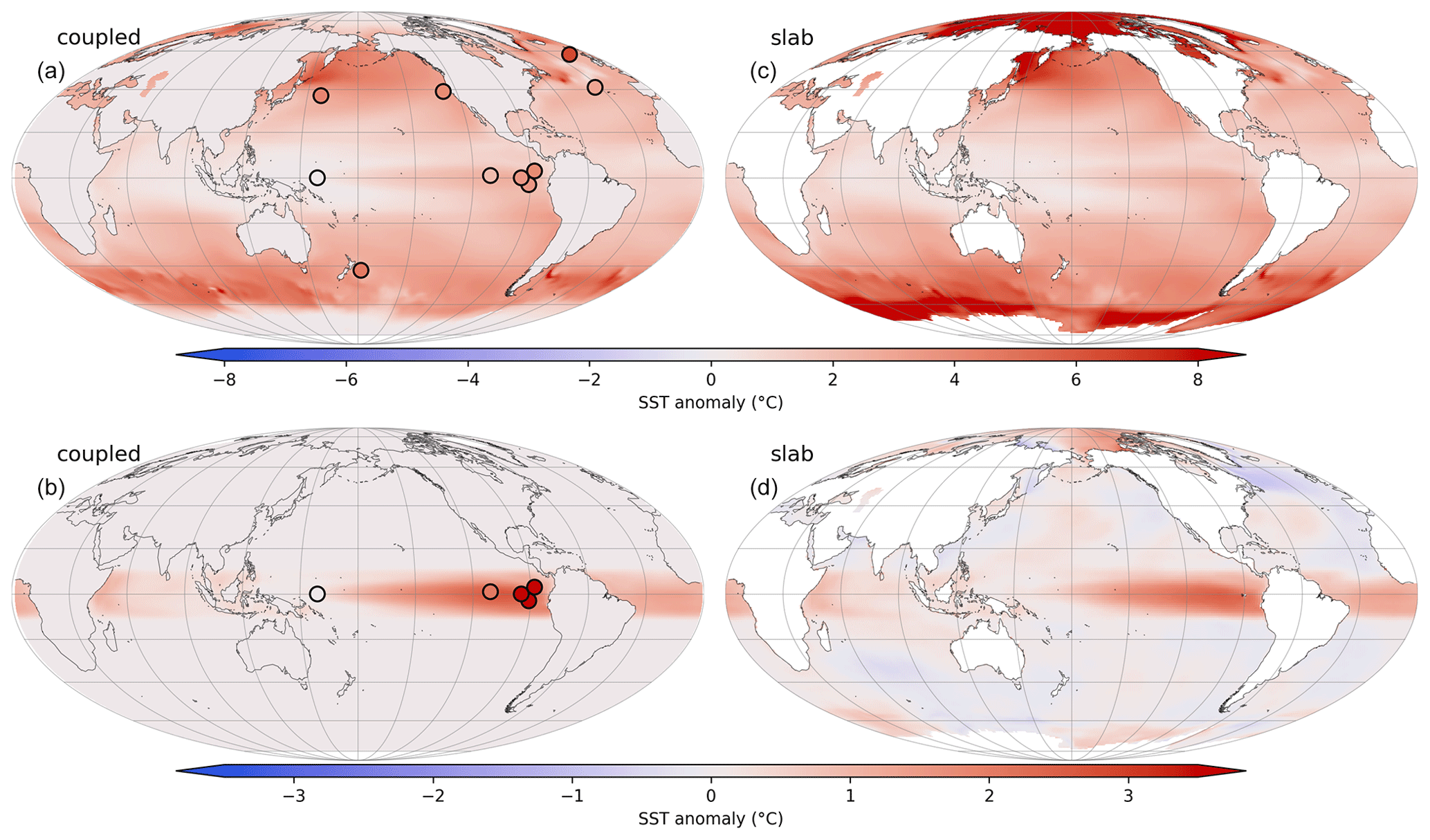
Figure 4Anomaly of SST (a, b) and ocean skin temperature – i.e., SST, except at grid points with sea ice (c, d). (a) Coupled ocean–atmosphere simulation with altered cloud properties (i.e., full Pliocene SST) for the pre-industrial CO2. (b) Same as (a) but the SST anomaly field is truncated at 10∘ N or S (i.e., 10∘ SN Pliocene SST). (c) Slab ocean simulation with Q flux derived to reproduce the full Pliocene SST (i.e., SST of panel a; CO2 at 300 ppmv). (d) Slab ocean simulation with Q flux derived to reproduce the 10∘ SN Pliocene SST (i.e., SST of panel b; CO2 at 299.4 ppmv). Note that the scale in (a) and (c) is different from (b) and (d). Colored dots in (a) and (b) are estimates of SST anomaly at 4.5–3.5 Ma from ODP proxies (see Appendix D). They follow the same color scale as their underlying map. Map projection and graticules are similar to Fig. 1. Large temperature anomalies (>8 ∘C) in (c) are found in regions influenced by sea ice and deviate from the original SST (panel a), which does not respond to the cloud albedo forcing (SST anomaly is 0 ∘C) because of the sea ice cover. Note that in (d), the temperature anomaly is not perfectly 0 ∘C outside 10∘ S–10∘ N because of inaccuracies in the derivation of the Q flux, but the amplitude of those anomalies is significantly less than within 10∘ S–10∘ N, with the exception of sea ice regions.
The slab ocean simulations reproduce the SST patterns well from the coupled ocean–atmosphere simulations, except in a few local spots. For instance, in Fig. 4b and d, it appears that the 10∘ SN Pliocene SST slab ocean simulation fails to generate a strictly null SST anomaly outside the 10∘ S–10∘ N band, but the magnitude of those subtropical anomalies is negligible compared to the expected ones within 10∘ S–10∘ N. Regions influenced by sea ice exhibit significant local differences, but they do not alter the global behavior of the simulations.
3.2.1 Weathering and equilibrium temperature with reduced zonal gradient
In this section, we examine the simulations where the Pliocene SST field is applied in the 10∘ S–10∘ N band (10∘ SN Pliocene SST) with the slab ocean version of CESM.
The standard CO2 experiment for this configuration (299.4 ppmv, see Appendix B, Sect. B2) has a global mean 2 m temperature of 13.67 ∘C, which is 0.25 ∘C warmer than the pre-industrial control (at 284.7 ppmv). The precipitation anomaly (Fig. 5a) exhibits a large increase in the eastern Pacific, similar to El Niño events. This increase does not extend southward as much as for observed El Niño conditions (Fig. 1b), likely because we imposed SST perturbation only in the 10∘ S–10∘ N band. Instead of drier conditions around the Maritime Continent and wetter conditions in the western Indian Ocean characteristic of El Niño, precipitation increases along the Equator (∘) across the Indian ocean and extends up to the eastern coast of Borneo over the Maritime Continent. The islands of Borneo, Sulawesi and New Guinea show a similar pattern of wetter conditions except on their western edge. The tropical Atlantic also shows significant differences with El Niño because the imposed SST in the Atlantic is warmer almost uniformly along the Equator (Fig. 4 b and d), which favors atmospheric convection. The runoff anomaly (Fig. 5a) reveals some similarities with the El Niño case (Fig. 1c): a decrease over India and Southeast Asia, an increase over China and the eastern side of the Himalaya, an increase in the Andes around the Equator, a decrease in the rest of equatorial South America (though the enhanced convection in the Atlantic generates wetter conditions along the Atlantic coast), an increase in the southeast part of South America, and an increase over the Congo basin. The largest discrepancies are found on the Maritime Continent and the East African Rift.
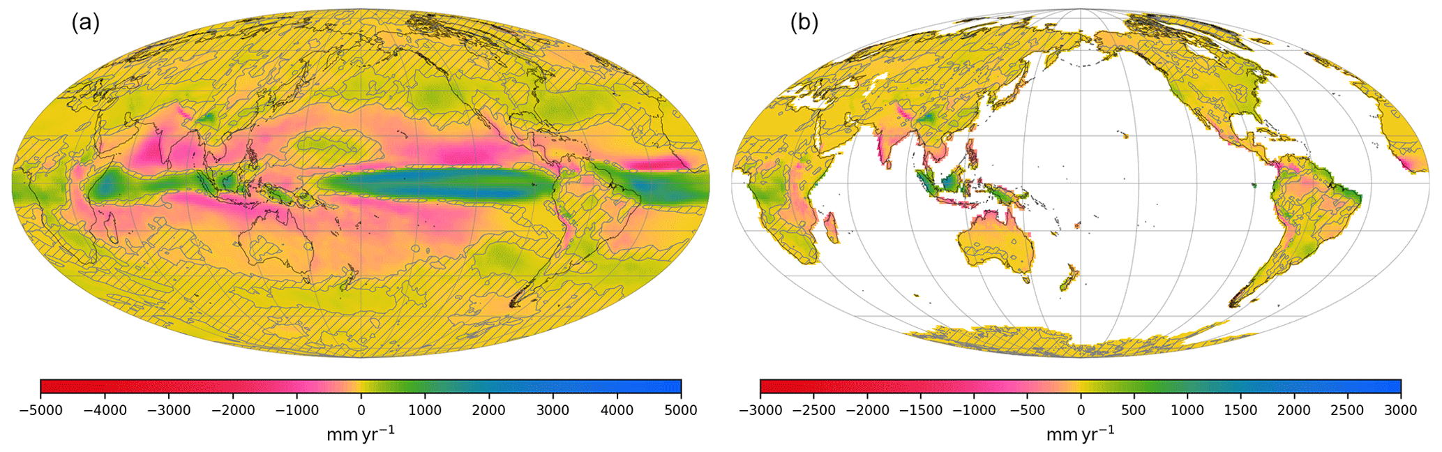
Figure 5Annual mean climatology of the slab ocean simulation with 10∘ SN Pliocene SST at 299.4 ppmv anomaly with respect to the pre-industrial control. (a) Total precipitation and (b) continental runoff. Map projection and graticules as in Fig. 1. In each panel, non-significant differences are hatched (p value of Welch's t test > 0.1, see Appendix C).
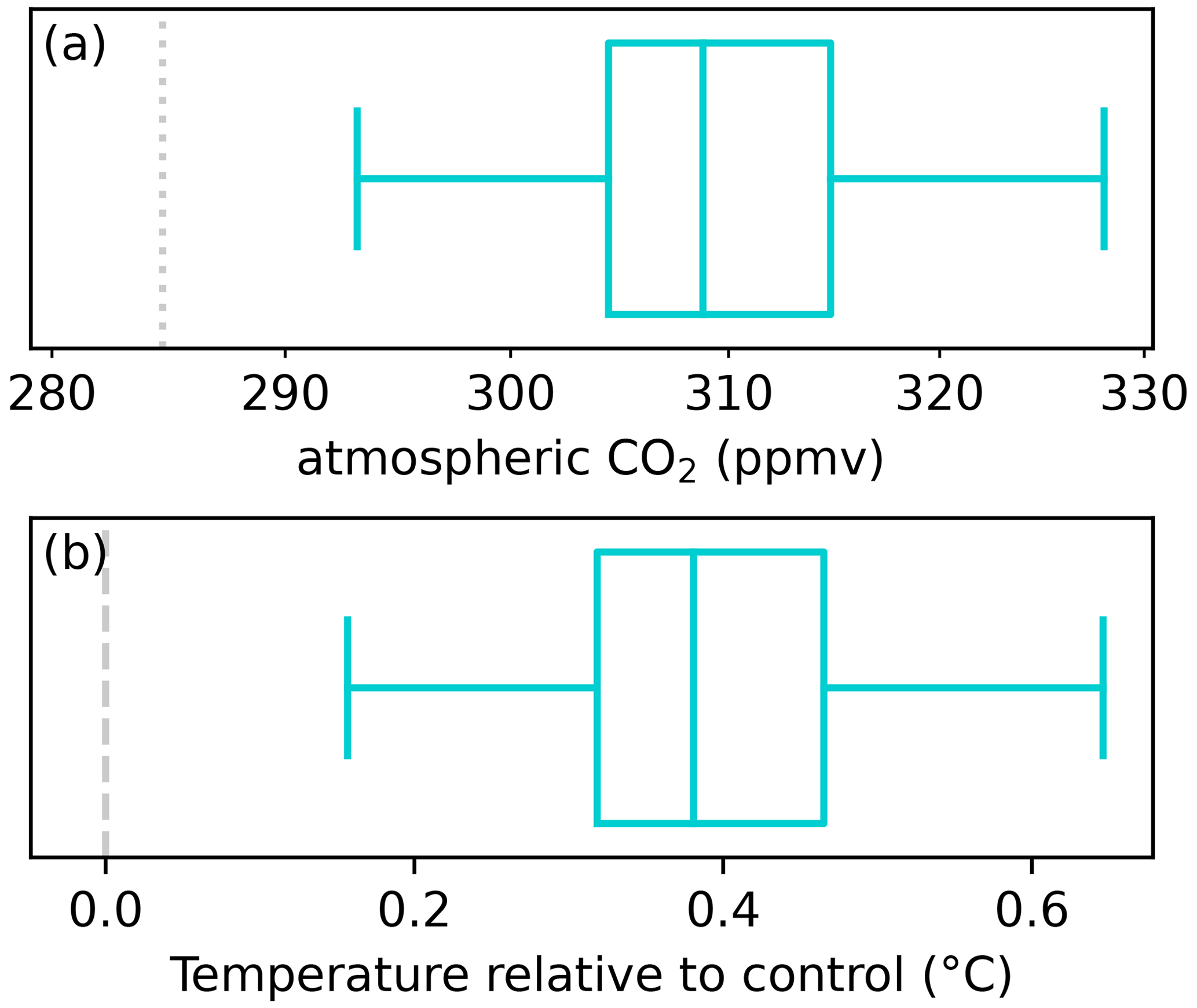
Figure 6Results for the 10∘ SN Pliocene SST GEOCLIM simulation at C cycle equilibrium (i.e., with silicate weathering flux balancing control degassing). (a) Atmospheric CO2 level (logarithmic axis) and (b) anomaly (with respect to pre-industrial simulation) of global mean 2 m temperature. The distribution – shown as a box plot – represents the ensemble of GEOCLIM parameterizations (similarly to Figs. 2c and 3c). The x axis of panel (a) is bounded so that a given CO2 in panel (a) corresponds to the aligned global temperature in panel (b). This is with the approximation that the CO2 is continuously logarithmic (from lower to upper bound), whereas GEOCLIM log(CO2) interpolates climate fields between the CO2 levels – the ones considered here being 250, 299.4 and 427.1 ppmv. Because of this approximation, the box plots in (a) and (b) are not perfectly aligned, but this misalignment is negligible. The pre-industrial CO2 level and the 0 ∘C anomaly are highlighted by the thin grey dashed or dotted vertical lines. Note that those two lines do not align because of the offset in the CO2–temperature relationship of the 10∘ SN Pliocene SST simulation with respect to the pre-industrial one.
We then used the 10∘ SN Pliocene SST simulations at several CO2 levels to compute the equilibrium CO2, which is the value at which the silicate weathering flux with 10∘ SN Pliocene SST balances CO2 degassing. More precisely, we consider control CO2 degassing to be equal to the pre-industrial silicate weathering flux. Therefore, for each selected combination of GEOCLIM parameters (see Methods, Sect. 2.1), we imposed the silicate weathering flux with 10∘ SN Pliocene SST as equal to the silicate weathering flux with the same parameter combination in the pre-industrial control simulation (i.e., computed with climate fields from pre-industrial slab simulation; this “control” weathering is shown in Fig. 2c, orange bars). Figure 6 shows this equilibrium CO2 (Fig. 6a) and the global mean 2 m temperature corresponding to that CO2 concentration (Fig. 6b). The Pliocene SST (within 10∘ S–10∘ N) generates climatic conditions less favorable for weathering, causing CO2 to increase and global temperature to rise by ∼0.4 ∘C, which is about twice that estimated using ERA5 reanalysis of El Niño years. This result is consistent with the fact that, in the 10∘ SN Pliocene SST simulation, the west-to-east Pacific SST difference is reduced by more (∼2.5∘) than in the climatology of El Niño years (∼1.5∘). Note that though the climate sensitivity (global temperature difference for a CO2 doubling) stays the same, there is an offset in the CO2–temperature relationship, meaning that CO2 of 284.7 ppmv does not correspond to a 0 ∘C temperature anomaly (see also Fig. 8a).
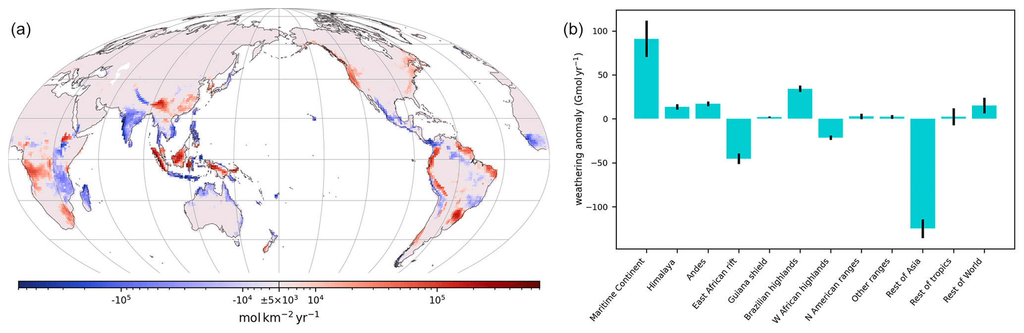
Figure 7(a) Anomaly of the weathering rate of the slab ocean climate simulation with 10∘ SN Pliocene SST at 299.4 ppmv with respect to pre-industrial control (averaged over the parameter combinations, similar to Fig. 3). (b) Bar plot of the anomaly of weathering flux from panel (a) integrated over the geographic regions (similar to Fig. 3c).
This decrease in weatherability (or weathering efficiency) can be investigated by looking at the anomaly of the silicate weathering rate of 10∘ SN Pliocene SST at 299.4 ppmv with respect to the pre-industrial control weathering rate (Fig. 7). Though the global temperature is not the same (10∘ SN Pliocene SST is 0.25∘ C warmer), it still illustrates the causes of this decrease in weatherability. Similar to what was observed with El Niño and La Niña composites (Fig. 3), several positive and negative regional anomalies of weathering, driven by runoff changes, compensate for each other, leading to a weak warming. Nevertheless, this warming is consistent over the whole ensemble of parameter combinations. Figure 7b shows the integration of the weathering rate anomaly from Fig. 7a over the geographic regions presented in Fig. 2a. Unlike the El Niño case, the weathering anomaly integrated over the Maritime Continent is positive, thereby not contributing to the warming. Indeed, there are more increases than decreases in runoff on the Maritime Continent in the 10∘ SN Pliocene SST simulation. The East African Rift also has an opposite behavior, with a decrease in weathering instead of a slight increase with El Niño. The last main difference concerns the category “the rest of Asia”, showing a large decrease in weathering. The decrease in runoff in India and associated weathering decrease overwhelm the increase in China, whereas those two balance out under modern El Niño conditions.
The weatherability decrease in the 10∘ SN Pliocene SST simulation can also be appreciated by looking at the global temperature–total weathering flux relationship (Fig. 8b). The 10∘ SN Pliocene SST curve (dashed blue) is systemically beneath the pre-industrial one (solid black) for any given global temperature. This means that regardless of the chosen background CO2 degassing flux, the simulation with 10∘ SN Pliocene SST will be warmer.
In summary, applying our estimation of Pliocene SST in the 10∘ S–10∘ N band – whose main feature is a flattening the tropical Pacific zonal gradient – generates a similar weatherability decrease and global warming to that estimated from El Niño (Sect. 3.1.2), though it is approximately twice as large. However, the mechanisms of that weatherability decrease are different due to differences in the regional patterns of simulated runoff.
3.2.2 Simulation with full Pliocene sea surface temperature
We now examine the slab ocean climate simulations wherein the full Pliocene SST field is applied. The most noticeable feature of the full Pliocene SST simulation is its mean temperature anomaly. As shown in Fig. 8a, for any given CO2 level, the full Pliocene SST slab ocean simulation is about 2.5 ∘C warmer than its counterpart with pre-industrial boundary conditions.
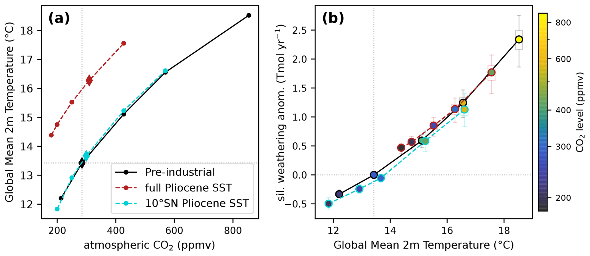
Figure 8(a) Global mean 2 m temperature (GMST) plotted against atmospheric CO2 level for the three series of slab ocean general circulation model (GCM) simulations: pre-industrial boundary conditions, full Pliocene SST and 10∘ SN Pliocene SST. Each dot represents an actual simulation, and the diamonds correspond to the “standard” CO2 levels (284.7 ppmv for pre-industrial; see the previous section for Pliocene SST). (b) Total silicate weathering flux anomaly (with respect to pre-industrial) plotted against GMST for the same three series of slab ocean GCM simulations (same color code as panel a). Each circle represents a single simulation at fixed CO2, with its level indicated by the color scale. The semi-transparent box plots show, for each simulation, the variability of weathering across the parameter combinations. In each panel, null weathering anomaly, pre-industrial GMST and pre-industrial CO2 level are highlighted by the vertical and horizontal thin grey dotted lines.
These warmer conditions at a given CO2 level can be explained by analyzing the components of the radiative budget. Figure 9 shows the comparison between the full Pliocene SST simulation and pre-industrial simulations interpolated at 309.4 ppmv (same CO2 level as Pliocene SST simulation) and at 538.3 ppmv (CO2 level at which the global mean 2 m temperature equals the one of the Pliocene SST simulation). A significant signal of the full Pliocene SST simulation can be found in the net solar radiative flux at the top of the atmosphere (Fig. 9a and e). There are two peaks of incoming radiation in the tropics (around 5∘ N and 10∘ S, Fig. 9e), which do not appear just by raising CO2 with pre-industrial boundary conditions. Such tropical peaks are caused by reduced cloudiness (Fig. 9d and h) due to less intense convection because of the reduced zonal temperature gradient, lowering Earth's shortwave albedo. Indeed, the cloud contribution to the peaks, estimated by the difference “full sky” minus “clear sky” (dashed lines in Fig. 9e), is almost 100 % of the signal. The SST pattern effect on global cloud radiative feedback has indeed been recognized (e.g., Zhou et al., 2017). Another peak in incoming solar radiation can be seen around 40∘ N or S Fig. 9e and corresponds to a poleward shift in cloudiness at those latitudes (Fig. 9d), mostly discernable in the Southern Hemisphere. This feature, however, is also found in the pre-industrial simulation at 538.3 ppmv and may be a mere consequence of rising global temperature, though its amplitude is higher in the full Pliocene SST simulation. More solar radiation also enters at high latitude in the Pliocene simulations relative to the pre-industrial control due to the retreat of sea ice, also lowering shortwave albedo. Though it is countered by an increase in cloudiness (Fig. 9d and h), as can be seen in the cloud contribution in Fig. 9e, the net effect is still positive. Similar to the peak at 40∘ N or S, this phenomenon is also present in the pre-industrial 538.3 ppmv simulation but is strengthened in the Pliocene SST simulation. On global average, the net solar radiation forcing of the full Pliocene simulation (with respect to pre-industrial at same CO2) is +3.9 W m−2, the tropical part alone being equivalent to +1.0 W m−2 (equivalent if spread over the whole Earth). The latitude profile of downwelling longwave radiation at Earth's surface also shows some variations (Fig. 9 b and f), essentially following the anomaly of water vapor (Fig. 9c and g). The reduced meridional temperature gradient in the full Pliocene SST simulation is responsible for less water vapor in the tropics and more water vapor in the extratropics compared to the pre-industrial simulation at the same mean temperature (Fig. 9g), though it is mostly visible in the Southern Hemisphere. The downwelling longwave radiation at the surface exhibits the same behavior. The more significant drops in the tropics (still compared to the pre-industrial simulation at the same mean temperature) are likely due to the reduced Hadley circulation. The averaged downwelling longwave flux anomaly is not so different between the Pliocene SST simulation and the pre-industrial one at 538.3 ppmv (+14.0 and +15.8 W m−2, respectively); both seem to be a consequence of a warmer atmosphere (and amplifier through a positive feedback loop). In summary, we can conclude that the main warming cause of the full Pliocene SST simulation is the decrease in cloudiness in the tropics due to a weaker convection and Hadley circulation, combined with a decrease in cloudiness around 40∘ N and S and of sea ice at high latitude, these last two also being part of a positive feedback enhancing the “initial” warming.
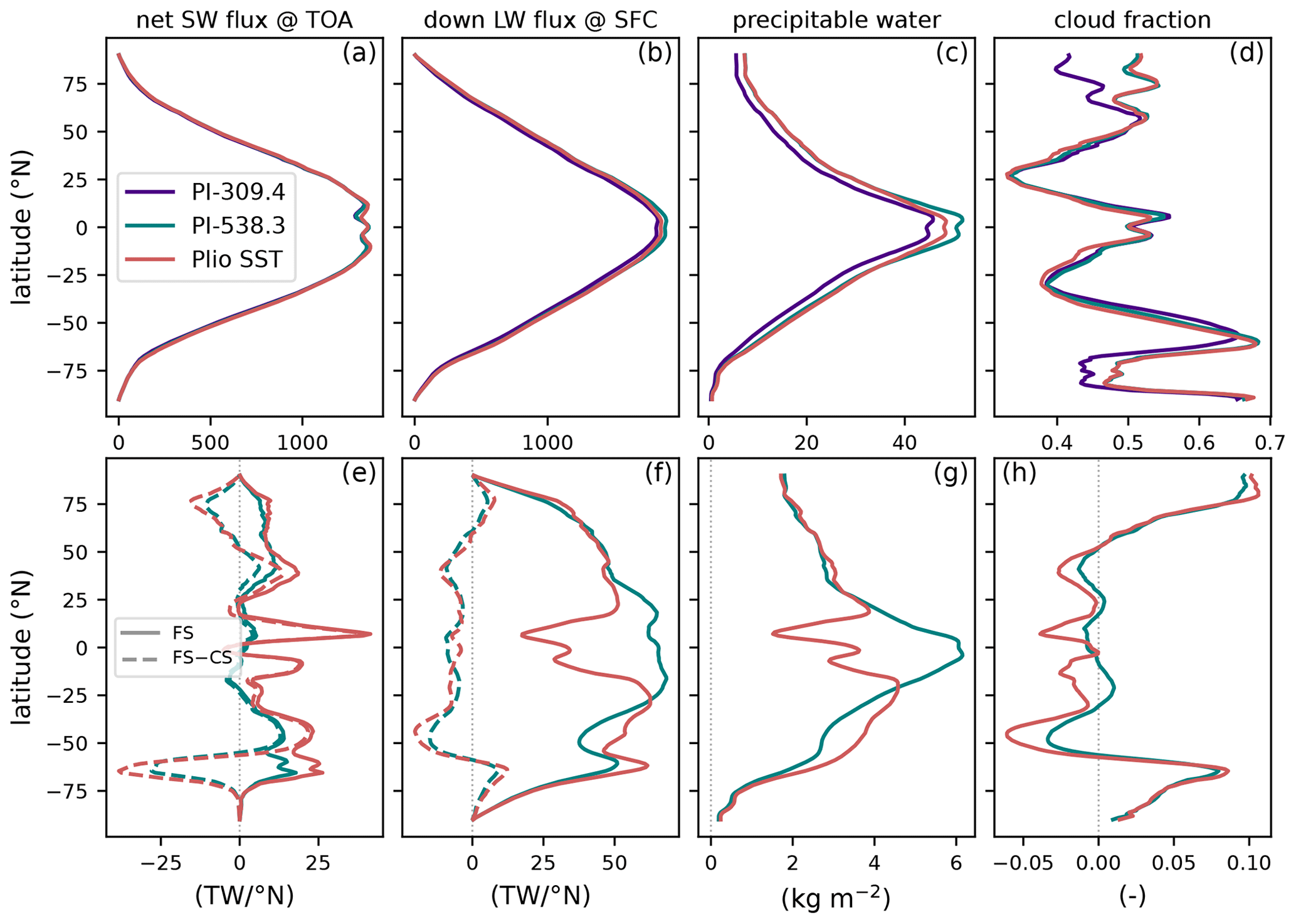
Figure 9Comparison of zonal annual mean fluxes and climatology for the three simulations, which are pre-industrial boundary conditions log (CO2 interpolated at 309.4 ppmv (indigo) or at 538.3 ppmv (teal) and full Pliocene SST (at 309.4 ppmv). (a) Zonally integrated net (incoming minus outgoing) solar (SW) radiative flux at the top of the atmosphere (TOA), (b) zonally integrated downwelling longwave (LW) radiative flux at the Earth's surface (SFC), (c) zonally averaged total precipitable water (vertically integrated) and (d) zonally averaged total cloud fraction (vertically integrated). All variables are annual mean climatology. Panels (e, f, g, h) are similar to (a–d) (respectively) but with 309.4 ppmv pre-industrial subtracted; the thin vertical grey dashed line highlights zero anomaly. The dashed color lines in (e) and (f) show the difference of full sky (SF) minus clear sky (CS), illustrating the contribution from clouds. The solid lines (full sky) are the regular values, as in (a) and (b). The “0 anomaly” in panels (e)–(h) is highlighted by a thin grey dotted vertical line. The color code holds for the entire figure.
In term of precipitation, it is easier to compare the full Pliocene SST simulation with the pre-industrial simulation log(CO2)-interpolated at the same global temperature to cancel the effect of increased precipitation with global warming. This precipitation (and runoff) difference is shown in Fig. 10. A redistribution of precipitation, with a decrease in the tropics and an increase in the extratropics, can be observed, superimposed on the anomalies already observed in the 10∘ SN Pliocene SST simulation (Fig. 5): an increase in the eastern tropical Pacific and on the western boundaries of the tropical Indian and Atlantic oceans. The results are different for land precipitation. Despite the reduced meridional temperature gradient, precipitation and runoff mostly increase in tropical Africa and South America, with the exception of the western part of the Amazon basin and the East African Rift, where a drying tendency was already observed in the 10∘ SN Pliocene SST simulation. This goes against our initial hypothesis based on the “wet gets drier, dry gets wetter” feature from Burls and Fedorov (2017). The Maritime Continent exhibits contrasting behavior, with wetter conditions on the western sides of the most equatorial islands and drier conditions on their eastern side. Such behavior was also present in the 10∘ SN Pliocene SST simulation, with a larger precipitation increase on the western sides, but is highlighted here because the anomaly is computed with respect to the pre-industrial simulation at 538.3 ppmv instead of 284.7 ppmv: the increase on the eastern sides is less than the roughly uniform increase due to higher CO2, whereas the increase on the western sides is larger. On global average, precipitation increases by 15 mm yr−1 and continental runoff increases by 16 mm yr−1.
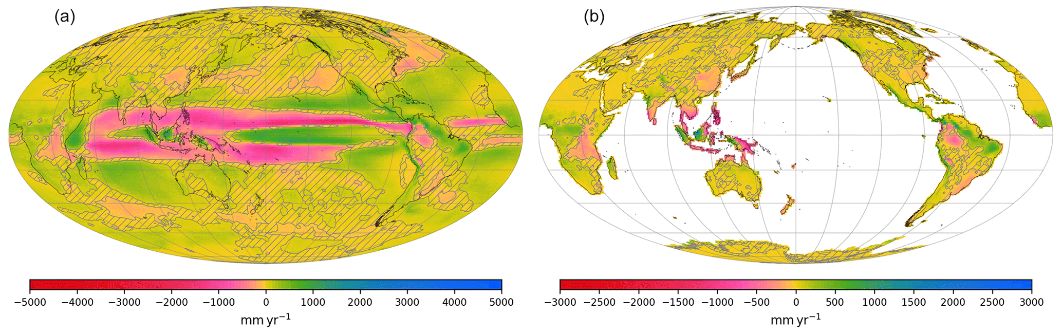
Figure 10Annual mean climatology of the slab ocean simulation with full Pliocene SST at 309.4 ppmv with respect to the pre-industrial control log (CO2)-interpolated at 358.3 ppmv. This last CO2 level was chosen so that the two simulations in the difference have the same global mean 2 m temperature. (a) Total precipitation and (b) continental runoff. Map projection and graticules are as in Fig. 1. In each panel, non-significant differences are hatched (p value of Welch's t test > 0.1, see Appendix C).
The offset in global temperature for a given CO2 level (in full Pliocene SST simulations with respect to pre-industrial ones) poses a technical problem: to go back down to pre-industrial temperature, with full Pliocene SST, CO2 needs to be lowered to ∼140 ppmv. Such CO2 levels are unrealistically low and are even lower than those during Pleistocene glacial maxima. Moreover, at this CO2 level, plant stomates cease to operate normally in the land model of CESM, with huge consequences for the hydrologic cycle. Shut stomate behavior contrasts with the regular tendency for stomates, which is to be more open at lower CO2, and severely reduces transpiration, eventually leading to increased global runoff, though the mean temperature is lower. Therefore, it is not possible to properly simulate silicate weathering with GEOCLIM. Increased runoff would lead to increased weathering at lower CO2 (thereby killing the negative feedback). This effect is likely responsible for the “flattening” of the temperature–weathering curve at the lowest tested CO2 levels (dashed red curve in Fig. 8b). On the other hand, the fact that plants cannot survive would undermine weathering, as plant roots are a major weathering agent. One may expect this second effect to be stronger and hence to see a collapse of total weathering flux with even lower CO2. For this reason, we cannot perform the inversion to compute the equilibrium CO2 wherein silicate weathering flux balances pre-industrial degassing. We instead analyze the weathering fluxes at fixed CO2.
Figure 8b illustrates the silicate weathering fluxes of the pre-industrial (solid black curve) and full Pliocene SST (dashed red curve) simulations. Despite the higher continental runoff compared to the pre-industrial simulation at the same global temperature, the full Pliocene SST temperature–weathering curve and the pre-industrial curve are superimposed, except for very low CO2 (<200 ppmv) Pliocene simulations. This result means that Pliocene SST does not generate any significant increase or decrease in weatherability – except at low CO2, but this is likely due to CO2–plant interaction and stomate closure that generates higher runoff. If the carbon cycle was left to reach balance, with pre-industrial degassing, CO2 would decrease, but it is not possible to determine what would be the equilibrium temperature. The dashed red curves in Fig. 8b cannot be extrapolated to the lower bound because it would fall outside the range of validity of the weathering model.
The fact that higher mean runoff does not lead to higher weatherability means that the regions where runoff decreases matter more in terms of weathering. Comparing the full Pliocene SST simulation to the pre-industrial interpolated at the same global temperature (538.3 ppmv) reveals weathering decreases in the almost all of Southeast Asia, India, China, the East African Rift, and even the Brazilian highlands and the Himalaya (Fig. 11). The combined decrease in those regions – mostly the first four – is enough to counteract the increase in the rest of the tropical land masses (Africa and South America) and along most of the American Cordillera (from the Andes to the Cascade Range, Fig. 11a) as shown in Fig. 11b.
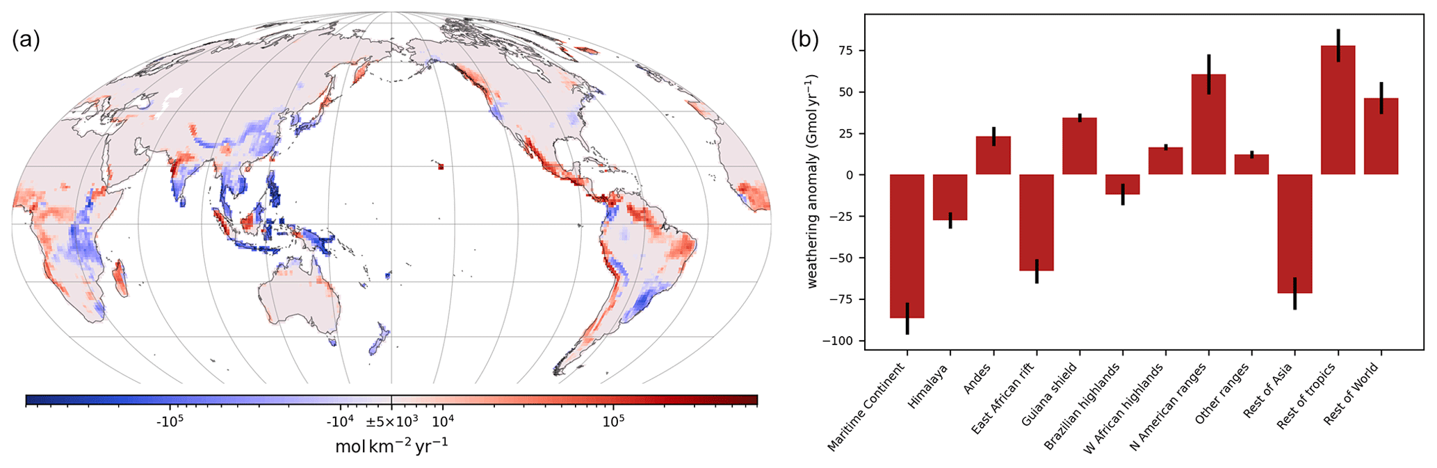
Figure 11(a) Anomaly of the weathering rate of the slab ocean climate simulation with full Pliocene SST at 309.4 ppmv; anomaly computed with respect to the pre-industrial simulation interpolated at 358.3 ppmv (see Fig. 10); (b) bar plot of the anomaly of weathering flux from panel (a).
Our results emphasize the different effects on silicate weathering of meridional and tropical zonal temperature gradients that are characteristic of Pliocene warmth, according to temperature proxies and the mechanistic connection between meridional and zonal SST gradients (Fedorov et al., 2015).
An estimate of the consequences of Pliocene permanent El Niño using reanalysis of modern El Niño events suggests a reduction of global weatherability by 1.7 %, which would correspond to a ∼0.23 ∘C warming relative to today (assuming a simple linear weathering feedback of ∼0.4 Tmol yr−1 ∘C−1 of global warming by CO2 that compensates for the +1.7 % weathering anomaly). Climate simulations with a permanent El Niño reconstruction of Pliocene SST in the 10∘ S–10∘ N band indicate a ∼0.4 ∘C warming relative to present-day conditions, but arising from different mechanisms. While El Niño reanalysis emphasized the role of the Maritime Continent in this warming through reduced weathering fluxes, climate simulations suggest, in contrast, a higher weathering flux in the Maritime Continent, offsetting the warming generated by the weathering decrease in mainland Southeast Asia, India and the East African Rift. Determining which of the two scenarios is the most reliable is not an easy task. Climate models contain biases, in particular for simulating precipitation. The way precipitation on the Maritime Continent is affected by SST changes in the CESM may not be accurate. Indeed, the fully coupled version of the climate model we used simulates rainfall increases in the winter and spring months over the Southeast Asian islands following peak El Niño, unlike the weak drying seen in observations (Deser et al., 2012, compare their Figs. 9 and 10). On the other hand, modern El Niño consists of transient events evolving over a period of a year with a peak in winter, not subject to the constraint of balancing Earth's radiative budget. These features differ from stationary (permanent) El Niño conditions, wherein the anomalously warm SSTs over the eastern equatorial Pacific occur for all months. Thus, modern-day El Niño events and their teleconnected impacts are likely to be quite different from those of a Pliocene permanent El Niño.
Nonetheless, the results agree on a modest warming effect (∼0.4 ∘C) of permanent El Niño resulting from a reduced global weatherability relative to the present day. Though its amplitude is small, this warming is robust across all weathering model parameterizations. However, this effect is not seen when the entire estimation of Pliocene SST is applied to the climate model. Further complications arise from the radiative budget of the Pliocene SST simulation that is ∼2.5 ∘C warmer than pre-industrial for a given CO2 level. This temperature shift is mostly caused by lower shortwave albedo due to fewer clouds in the tropics, as well as a poleward shift in the midlatitude peak of cloudiness, and reduced sea ice. If a flatter meridional temperature gradient is the result of warmer global temperature (due to higher CO2), a direct consequence would be that climate sensitivity to CO2 is much higher than current estimates. This raises the question of how representative of Pliocene SST our reconstruction is using the Burls and Fedorov (2014) method – modifying cloud shortwave albedo – though it is globally in agreement with SST proxies.
The larger lesson we learn from our simulations is that SST pattern changes result in large regional changes in weathering of both signs. They tend to cancel each other out, but depending on the SST pattern there can still be a significant warming effect, as seen in the permanent El Niño and 10∘ S–10∘ N Pliocene SST cases. While the effect of reduced meridional SST gradient seems to cancel the reduced tropical zonal SST gradient in our Pliocene SST simulation by increasing mean precipitation and continental runoff, this cancellation could be seen as fortuitous, and a different magnitude of the reduced meridional SST gradient could give rise to a net effect. A proper evaluation of the weatherability pattern effect for the Pliocene thus requires a robust SST reconstruction for that time period.
Long-term cooling of Earth's climate from the mid-Miocene to the present associated with decreasing CO2 likely resulted from increased weatherability (e.g., Park et al., 2020), decreased outgassing (e.g., Herbert et al., 2022, though no clear change is noted since the Pliocene) or a combination of the two. Superimposed on this long-term trend are large changes in climate dynamics whose impacts on regional climatology could play an important role in processes such as the growth of Northern Hemisphere ice sheets (e.g., Molnar and Cronin, 2015). Additionally, regional changes in precipitation and runoff could alter silicate weathering with resulting implications for geologic carbon sequestration and steady-state CO2 levels. We coin this phenomenon the “weatherability pattern effect”, analogous to the pattern effect in climate sensitivity. In this contribution, we investigated the weatherability pattern effect due to SST gradients. We both put forward and evaluate the hypothesis that the transition from a Pliocene permanent El Niño climate to a modern El Niño–Southern Oscillation climate could be associated with an increase in weatherability due to shifts in precipitation to or from chemical weathering hotspots. We explored this hypothesis by running a chemical weathering model with El Niño climate as found in reanalysis data and by climate model simulations imposing Pliocene-like SST changes. Significant regional changes in both signs are found in the weathering patterns of the different experiments, particularly in tropical weathering hotspots. These changes largely cancel but can produce a modest but significant weatherability increase should they not entirely compensate. These results highlight the potential importance of the weatherability pattern effect on Earth's long-term carbon cycle, though a proper evaluation requires a robust reconstruction of the relevant SST patterns.
We generated the ENSO index from the climate fields from ERA5 reanalysis (1979–2020 time series) as follows: we used the detrended monthly SST average for the Niño 3 region, which is 5∘ N–5∘ S, 150–90∘ W (Trenberth and Stepaniak, 2001). We detrended the time series by performing a linear regression with respect to time and subtracted the “time” term from the original time series. We grouped the monthly time series in “year” vectors of 12 elements, corresponding to the 12 months, from May to April of the next calendar year. We subtracted from each year vector the average of all years to center the vectorial time series. We then performed a principal component analysis. We identified the first eigenvector (or EOF for empirical orthogonal function) as the signature of El Niño events. We projected the detrended, centered, vectorial time series on this first EOF (scalar product of the two 12-element vectors for each year). We normalized the scalar time series obtained in this way by dividing it by its standard deviation (across the years). This normalized time series can be interpreted as a time series of the El Niño index for each year. We selected the El Niño years as the years having an index > 0.9 and for the La Niña years.
The resulting ENSO index yearly time series is shown in Fig. A1.
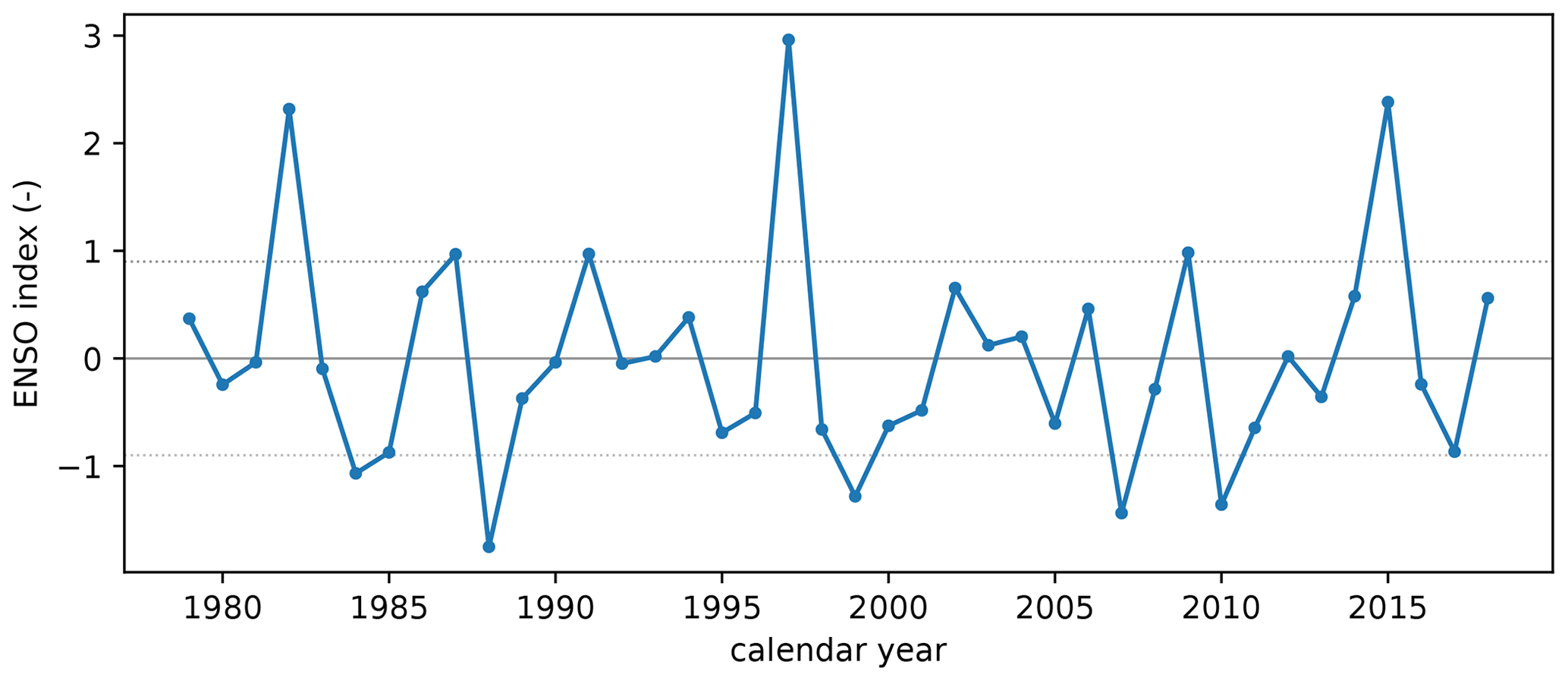
Figure A1Time series of the calculated ENSO index. The horizontal lines highlight the 0 value as well as the threshold values of 0.9 and −0.9 chosen for El Niño and La Niña years, respectively.
The aim of the following procedure is to generate slab ocean climate simulations – at several CO2 levels – with SST patterns that replicate the meridional and tropical zonal gradients presented in Burls and Fedorov (2014, 2017) and Fedorov et al. (2015). We proceeded in three steps.
B1 Full ocean simulations at pre-industrial CO2
For this step, we strictly applied the method of Burls and Fedorov (2014) in an attempt to reproduce Pliocene SST. From this simulation, we will only consider the SST field.
In the ocean–atmosphere coupled version of CESM1.2, we modified the cloud shortwave albedo by changing the value of the water path in the radiative code of CAM4. The cloud liquid and solid water path was multiplied by 3.4 between 15∘ N north and south, and the cloud liquid water path was multiplied by 0.4 for the rest of the Earth. We ran those simulations for 230 years, which is sufficient for the surface ocean to respond to the perturbation (Fedorov et al., 2015). At this point, we are not interested in accurately reaching the radiative equilibrium. The last 30 years of simulation were used to extract the SST field. This field exhibits the features of reduced zonal and meridional gradients, in accordance with Burls and Fedorov (2014). We refer to this SST field as the full Pliocene SST. We also ran a pre-industrial control simulation for 170 years, taking the last 30 years to extract the pre-industrial control SST field. Finally, in order to create a Pliocene SST field for the tropics only, we merged the full Pliocene SST in the tropics with the pre-industrial control SST in the extratropics using
where
with latitude in degrees. We refer to this SST field as the 10∘ SN Pliocene SST.
B2 Fixed-SST simulations with zero-integral net ocean–atmosphere heat flux
In this second step, we took the pre-industrial control SST, the full Pliocene SST and the 10∘ SN Pliocene SST fields and ran atmosphere-only (i.e., fixed-SST) simulations for each of those fields.
Table B1Summary of all the climate simulations used for the present study (including “intermediate” simulations) and the specificity of their design.
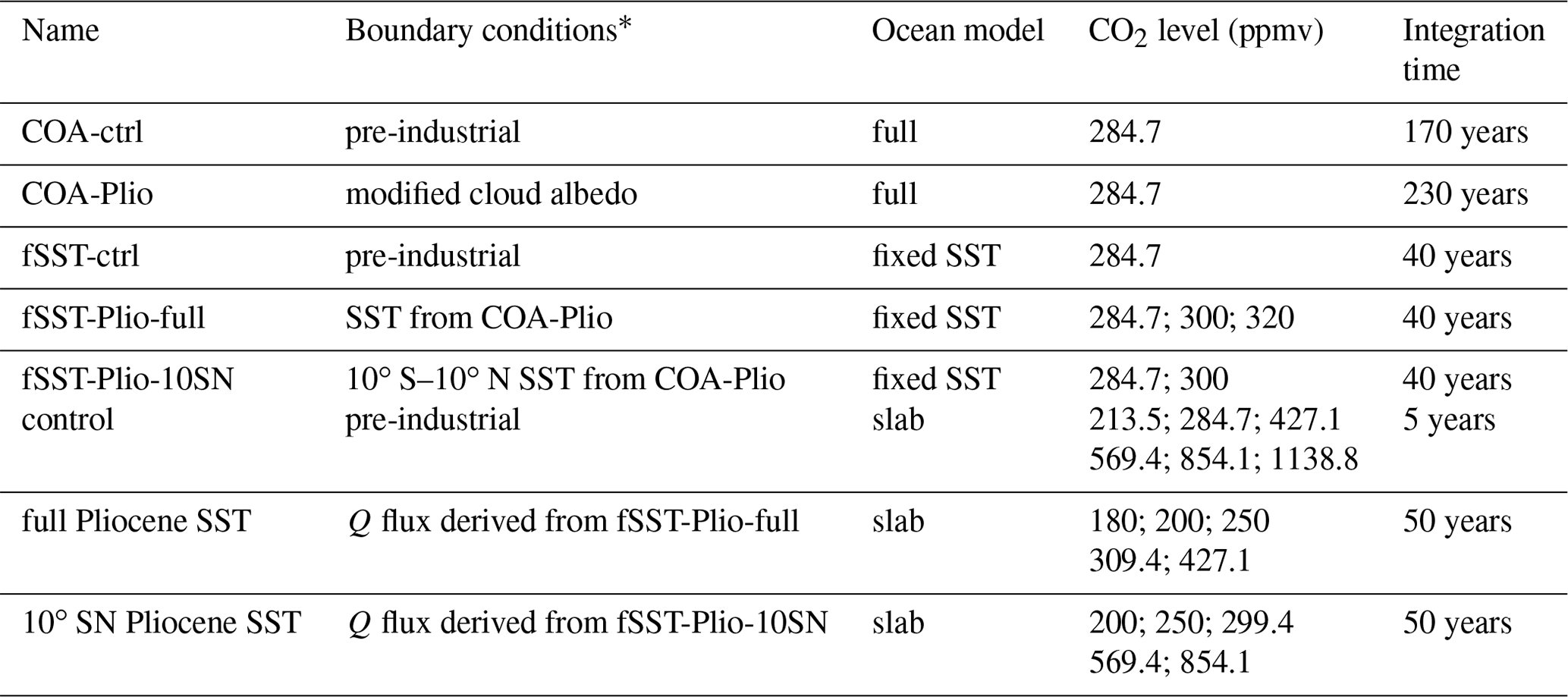
* Refers to all climate model boundary conditions except atmospheric CO2. Anything other than the indicated modifications is pre-industrial
Note that we use the standard CAM4 model for each simulation (i.e., we do not alter the cloud properties) so that the climate model physics are consistent. Those simulations were run at several CO2 levels (284.7, 300 and 320 ppmv for the full Pliocene SST; 284.7 and 300 ppmv for the 10∘ SN Pliocene SST). We did so in order to estimate at which CO2 level the atmosphere is in equilibrium with the SST, meaning that the net surface heat flux (Fnet, Eq. B3) sums at zero. We estimated those CO2 levels as 309.4 ppmv for the full Pliocene SST and 299.4 ppmv for the 10∘ SN Pliocene SST by linearly interpolation Fnet as a function of log (CO2). Fnet is computed as
where FSW is the net (downward) solar flux, FLW is net (upward) longwave flux, FL is the latent heat flux and FS the sensible heat flux, which are all fluxes at the Earth's surface. These atmosphere-only simulations were run for 40 years, and the last 30 years were used to extract Fnet.
B3 Slab ocean simulations with Pliocene SST
In this last step, we used zero-sum Fnet from the full and 10∘ SN Pliocene SST atmosphere-only simulations to derive oceanic Q flux: Q. The Q flux refers to the forcing term of a slab ocean model. It represents the divergence of oceanic heat transport and directly controls the warming or cooling of the surface ocean in a slab model.
We computed the Q flux for each month of the annual cycle with the following equation:
where ρwat is the seawater density, is the seawater heat capacity, hml is the depth of ocean mixed layer, ρice is the density of sea ice, Lfus is the latent heat of fusion of water, hice is the thickness of sea ice and xice is the fraction of each oceanic grid covered by sea ice. The time derivative was approximated here as the month-by-month finite difference. The mixed layer depth hml was taken from the default pre-industrial Q flux forcing (see Methods, Sect. 2.3) and is time-invariant. The SST and ice fraction (xice) were taken from the Pliocene SST atmosphere-only simulations (full or 10∘ SN).
More precisely, we computed the anomaly of SST, xice and Fnet by subtracting the fields taken from Pliocene SST atmosphere-only simulations from the fields from the pre-industrial control atmosphere-only climate run. Noting this subtraction Δ, we actually computed ΔQ as
With ΔQ thus calculated, the Pliocene Q flux was computed as Qcontrol+ΔQ (for both full SST and 10∘ SN SST fields). Using this generated Q flux, we ran climate simulations with the slab ocean version of CESM1.2 at the “standard” CO2 level (309.4 or 299.4 ppmv, see previous paragraph) and at higher or lower CO2 (180, 200, 250, 427.1 and 569.4 ppmv) to encompass the full range of climate warming or cooling, as CO2 must adjust to balance the geological C cycle. Here again, the standard CAM4 model is used in all instances so that the climate model physics are consistent.
The least-constrained variable here is the sea ice thickness (hice). In the absence of information, as it cannot be retrieved from the atmosphere-only simulations, we assumed a constant, uniform thickness of 1 m. Despite this crude assumption, the slab ocean simulations (at standard CO2) reproduce the SST fields from the original ocean–atmosphere coupled model well (see Fig. 4).
We note that these estimated CO2 levels that balance the heat flux in the atmosphere-only simulations are different from the C cycle equilibrium CO2 levels computed by GEOCLIM. The former is done so that the derived Q flux change does not artificially introduce heat into or out of the ocean. With a slab ocean model, the null Fnet condition is verified for any CO2 level because it is imposed by the Q flux. The latter CO2 levels computed by GEOCLIM are the ones that balance the geologic C cycle.
Finally, we ran full Pliocene SST and 10∘ SN Pliocene SST slab ocean simulations at several CO2 levels using the Q fluxes thus generated. Table B1 summarizes all the climate simulations that were conducted for this study. The slab ocean simulations (last two entries of Table B1) are the main focus of the article; the other simulations are intermediate simulations needed to design the slab ocean simulations.
Figures 1, 5 and 10 include statistical tests to determine statistically significant patterns in the anomalies. In every case, a Welch's t test was performed to compare the control and the perturbed fields (temperature, precipitation or runoff). For those tests, we considered samples of annual means (i.e., 1-year average), where every year is assumed to be an independent observation. Hence, the variance estimates used for the tests are the empirical variance between the years. The null hypothesis of the test is that the control and perturbed averages (i.e., average of all the 1-year annual means) are equal.
For the CESM simulations, the control population is the 30-year climatology of the pre-industrial simulation, and the perturbed populations are the 30-year climatology of either the 10∘ SN Pliocene SST (Fig. 5) or full Pliocene SST (Fig. 10) simulations. The sample size N is 30 for both the control and perturbed populations.
For the ERA5 reanalysis (Fig. 1), the test we performed is meant to compare the selected El Niño years and the regular years. Therefore, the control population is the sample of all the years (from May to the following April) whose ENSO index exceeds neither the El Niño nor the La Niña threshold (sample size N=29) and the perturbed population is the sample of El Niño years (sample size N=6).
We used an alkenone SST proxy (U) from ODP sites 1125 (Fedorov et al., 2015), 850, 806 (Zhang et al., 2014), 1208, 1021 (LaRiviere et al., 2012), 607, 856, 847, 982 and 1241 (Brierley et al., 2009). For each site, we averaged the available SST estimates between 4.5 and 3.5 Ma as “Pliocene” SST. In the case of Brierley et al. (2009) (sites 607, 856, 847, 982 and 1241), we took the SST already averaged in Table S1 of their contribution (local SST without correction). For the control SST values, we used the modern SST from Fedorov et al. (2015) in Table S1 of their contribution. There are two exceptions: for sites 1021 and 806, we considered the near-modern interglacial SST of the time series to be the modern SST because they significantly differ from the actual modern SST (Fedorov et al., 2015, Table S1).
Fedorov et al. (2015)Zhang et al. (2014)Zhang et al. (2014)LaRiviere et al. (2012)LaRiviere et al. (2012)Brierley et al. (2009)Brierley et al. (2009)Brierley et al. (2009)Brierley et al. (2009)Brierley et al. (2009)Table D1Details of SST proxies shown in the present study.
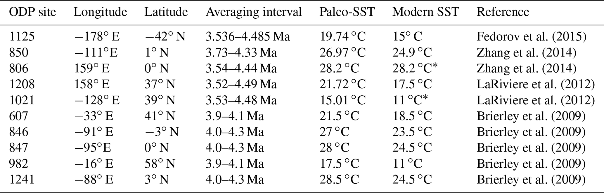
* Taken from the SST proxy time series (see text).
All code associated with this study is archived on Zenodo (https://doi.org/10.5281/zenodo.8013407, Maffre et al., 2023a).
All climate and GEOCLIM simulations used for this study are available in the following dataset: Maffre et al. (2023b) (https://doi.org/10.6078/D11H7D).
PM and JCHC conceived the experiments and ran the climate simulations. PM ran the GEOCLIM simulations, wrote the original paper draft, and drafted the figures. JCHC and NLSH contributed to paper writing. JCHC and NLSH acquired funding and supervised project research.
The contact author has declared that none of the authors has any competing interests.
Publisher's note: Copernicus Publications remains neutral with regard to jurisdictional claims in published maps and institutional affiliations.
Research was supported by NSF Frontier Research in Earth Science grant EAR-1925990 awarded to Nicholas L. Swanson-Hysell and John C. H. Chiang. We thank Natalie Burls for useful discussions on climate dynamics and guidance on the design and interpretation of the climate simulations. We dedicate this work to the memory of our dear colleague and friend Sarah White, whose work on permanent El Niño and its impacts inspired this paper.
This research has been supported by the National Science Foundation (grant no. EAR-1925990).
This paper was edited by Yannick Donnadieu and reviewed by three anonymous referees.
Berner, R. A., Lasaga, A. C., and Garrels, R. M.: The carbonate-silicate geochemical cycle and its effect on atmospheric carbon dioxide over the past 100 million years, Am. J. Sci., 283, 641–683, https://doi.org/10.2475/ajs.283.7.641, 1983. a
Brierley, C. M. and Fedorov, A. V.: Relative importance of meridional and zonal sea surface temperature gradients for the onset of the ice ages and Pliocene-Pleistocene climate evolution: SST GRADIENTS AND ICE AGES, Paleoceanography, 25, PA2214, https://doi.org/10.1029/2009PA001809, 2010. a
Brierley, C. M., Fedorov, A. V., Liu, Z., Herbert, T. D., Lawrence, K. T., and LaRiviere, J. P.: Greatly Expanded Tropical Warm Pool and Weakened Hadley Circulation in the Early Pliocene, Science, 323, 1714–1718, https://doi.org/10.1126/science.1167625, 2009. a, b, c, d, e, f, g, h
Burls, N. J. and Fedorov, A. V.: What Controls the Mean East–West Sea Surface Temperature Gradient in the Equatorial Pacific: The Role of Cloud Albedo, J. Climate, 27, 2757–2778, https://doi.org/10.1175/JCLI-D-13-00255.1, 2014. a, b, c, d, e, f, g, h, i
Burls, N. J. and Fedorov, A. V.: Wetter subtropics in a warmer world: Contrasting past and future hydrological cycles, P. Natl. Acad. Sci. USA, 114, 12888–12893, https://doi.org/10.1073/pnas.1703421114, 2017. a, b, c, d, e
Cannariato, K. G. and Ravelo, A. C.: Pliocene-Pleistocene evolution of eastern tropical Pacific surface water circulation and thermocline depth, Paleoceanography, 12, 805–820, https://doi.org/10.1029/97PA02514, 1997. a
Deser, C., Phillips, A. S., Tomas, R. A., Okumura, Y. M., Alexander, M. A., Capotondi, A., Scott, J. D., Kwon, Y.-O., and Ohba, M.: ENSO and Pacific Decadal Variability in the Community Climate System Model Version 4, J. Climate, 25, 2622–2651, https://doi.org/10.1175/JCLI-D-11-00301.1, 2012. a
Dessert, C., Dupré, B., Gaillardet, J., François, L. M., and Allègre, C. J.: Basalt weathering laws and the impact of basalt weathering on the global carbon cycle, Chem. Geol., 202, 257–273, https://doi.org/10.1016/j.chemgeo.2002.10.001, 2003. a
Farr, T. G., Rosen, P. A., Caro, E., Crippen, R., Duren, R., Hensley, S., Kobrick, M., Paller, M., Rodriguez, E., Roth, L., Seal, D., Shaffer, S., Shimada, J., Umland, J., Werner, M., Oskin, M., Burbank, D., and Alsdorf, D.: The Shuttle Radar Topography Mission, Rev. Geophys., 45, RG2004, https://doi.org/10.1029/2005RG000183, 2007. a
Fedorov, A. V., Dekens, P. S., McCarthy, M., Ravelo, A. C., deMenocal, P. B., Barreiro, M., Pacanowski, R. C., and Philander, S. G.: The Pliocene Paradox (Mechanisms for a Permanent El Niño), Science, 312, 1485–1489, https://doi.org/10.1126/science.1122666, 2006. a
Fedorov, A. V., Brierley, C. M., Lawrence, K. T., Liu, Z., Dekens, P. S., and Ravelo, A. C.: Patterns and mechanisms of early Pliocene warmth, Nature, 496, 43–49, https://doi.org/10.1038/nature12003, 2013. a, b
Fedorov, A. V., Burls, N. J., Lawrence, K. T., and Peterson, L. C.: Tightly linked zonal and meridional sea surface temperature gradients over the past five million years, Nat. Geosci., 8, 975–980, https://doi.org/10.1038/ngeo2577, 2015. a, b, c, d, e, f, g, h, i, j, k, l
Fekete, B. M., Vörösmarty, C. J., and Grabs, W.: Global, composite runoff fields based on observed river discharge and simulated water balances, Global Runoff Data Centre Koblenz, Germany, https://www.compositerunoff.sr.unh.edu/ (last access: 1 December 2019), 1999. a
Gabet, E. J. and Mudd, S. M.: A theoretical model coupling chemical weathering rates with denudation rates, Geology, 37, 151–154, https://doi.org/10.1130/G25270A.1, 2009. a
Gaillardet, J., Dupré, B., Louvat, P., and Allègre, C. J.: Global silicate weathering and CO2 consumption rates deduced from the chemistry of large rivers, Chem. Geol., 159, 3–30, https://doi.org/10.1016/S0009-2541(99)00031-5, 1999. a
Harris, I., Jones, P., Osborn, T., and Lister, D.: Updated high-resolution grids of monthly climatic observations - the CRU TS3.10 Dataset: Updated High-Resolution Grids Of Monthly Climatic Observations, Int. J. Climatol., 34, 623–642, https://doi.org/10.1002/joc.3711, 2014. a
Hartmann, J. and Moosdorf, N.: The new global lithological map database GLiM: A representation of rock properties at the Earth surface, Geochem. Geophy. Geosy., 13, Q12004, https://doi.org/10.1029/2012GC004370, 2012. a
Herbert, T. D., Dalton, C. A., Liu, Z., Salazar, A., Si, W., and Wilson, D. S.: Tectonic degassing drove global temperature trends since 20 Ma, Science, 377, 116–119, https://doi.org/10.1126/science.abl4353, 2022. a, b
Hersbach, H., Bell, B., Berrisford, P., Biavati, G., Horányi, A., Muñoz Sabater, J., Nicolas, J., Peubey, C., Radu, R., Rozum, I., Schepers, D., Simmons, A., Soci, C., Dee, D., and Thépaut, J.-N.: ERA5 monthly averaged data on single levels from 1979 to present, CDS, https://doi.org/10.24381/CDS.F17050D7, 2019. a, b
Kukla, T., Ibarra, D., Lau, K. V., and Rugenstein, J. K. C.: All aboard! Earth system investigations with the CH2O-CHOO TRAIN v1.0, EGUsphere [preprint], https://doi.org/10.5194/egusphere-2022-1000, 2022. a
Langenbrunner, B.: The pattern effect and climate sensitivity, Nat. Clim. Change, 10, 977–977, https://doi.org/10.1038/s41558-020-00946-y, 2020. a
LaRiviere, J. P., Ravelo, A. C., Crimmins, A., Dekens, P. S., Ford, H. L., Lyle, M., and Wara, M. W.: Late Miocene decoupling of oceanic warmth and atmospheric carbon dioxide forcing, Nature, 486, 97–100, https://doi.org/10.1038/nature11200, 2012. a, b, c
Maffre, P., Ladant, J.-B., Moquet, J.-S., Carretier, S., Labat, D., and Goddéris, Y.: Mountain ranges, climate and weathering. Do orogens strengthen or weaken the silicate weathering carbon sink?, Earth Planet. Sc. Lett., 493, 174–185, https://doi.org/10.1016/j.epsl.2018.04.034, 2018. a
Maffre, P., Swanson-Hysell, N., and Park, Y.: piermafrost/GEOCLIM-dynsoil-steady-state: version compatible with Maffre et al. (2023) Clim Past, Zenodo [code], https://doi.org/10.5281/zenodo.8013407, 2023a. a
Maffre, P., Chiang, J., and Swanson-Hysell, N.: Data for: The effect of Pliocene regional climate changes on silicate weathering, Dryad [data set], https://doi.org/10.6078/D11H7D, 2023b. a
Maher, K. and Chamberlain, C. P.: Hydrologic Regulation of Chemical Weathering and the Geologic Carbon Cycle, Science, 343, 1502–1504, https://doi.org/10.1126/science.1250770, 2014. a
Molnar, P. and Cane, M. A.: El Niño's tropical climate and teleconnections as a blueprint for pre-Ice Age climates., Paleoceanography, 17, 11-1–11-11, https://doi.org/10.1029/2001PA000663, 2002. a
Molnar, P. and Cronin, T. W.: Growth of the Maritime Continent and its possible contribution to recurring Ice Ages: Maritime Continent Growth and Ice Ages, Paleoceanography, 30, 196–225, https://doi.org/10.1002/2014PA002752, 2015. a, b, c
Muñoz Sabater, J.: ERA5-Land monthly averaged data from 2001 to present, CDS, https://doi.org/10.24381/CDS.68D2BB30, 2019. a, b
Oliva, P., Viers, J., and Dupré, B.: Chemical weathering in granitic environments, Chem. Geol., 202, 225–256, https://doi.org/10.1016/j.chemgeo.2002.08.001, 2003. a
Park, Y., Maffre, P., Goddéris, Y., Macdonald, F. A., Anttila, E. S. C., and Swanson-Hysell, N. L.: Emergence of the Southeast Asian islands as a driver for Neogene cooling, P. Natl. Acad. Sci. USA, 117, 25319–25326, https://doi.org/10.1073/pnas.2011033117, 2020. a, b, c, d, e, f, g
Ravelo, A. C.: The Role of the Tropical Oceans on Global Climate During a Warm Period and a Major Climate Transition, Oceanography, 17, 32–41, https://doi.org/10.5670/oceanog.2004.28, 2004. a
Shukla, S. P., Chandler, M. A., Jonas, J., Sohl, L. E., Mankoff, K., and Dowsett, H.: Impact of a permanent El Niño (El Padre) and Indian Ocean Dipole in warm Pliocene climates, Paleoceanography, 24, PA2221, https://doi.org/10.1029/2008PA001682, 2009. a
Trenberth, K. E. and Stepaniak, D. P.: Indices of El Niño Evolution, J. Climate, 14, 1697–1701, https://doi.org/10.1175/1520-0442(2001)014<1697:LIOENO>2.0.CO;2, 2001. a
Urey, H. C.: On the Early Chemical History of the Earth and the Origin of Life, P. Natl. Acad. Sci. USA, 38, 351–363, https://doi.org/10.1073/pnas.38.4.351, 1952. a
Walker, J. C. G., Hays, P. B., and Kasting, J. F.: A negative feedback mechanism for the long-term stabilization of Earth's surface temperature, J. Geophys. Res., 86, 9776, https://doi.org/10.1029/JC086iC10p09776, 1981. a, b
Wara, M. W., Ravelo, A. C., and Delaney, M. L.: Permanent El Niño-Like Conditions During the Pliocene Warm Period, Science, 309, 758–761, https://doi.org/10.1126/science.1112596, 2005. a
West, A. J.: Thickness of the chemical weathering zone and implications for erosional and climatic drivers of weathering and for carbon-cycle feedbacks, Geology, 40, 811–814, https://doi.org/10.1130/G33041.1, 2012. a
Zhang, Y. G., Pagani, M., and Liu, Z.: A 12-Million-Year Temperature History of the Tropical Pacific Ocean, Science, 344, 84–87, https://doi.org/10.1126/science.1246172, 2014. a, b, c
Zhou, C., Zelinka, M. D., and Klein, S. A.: Analyzing the dependence of global cloud feedback on the spatial pattern of sea surface temperature change with a Green's function approach, J. Adv. Model. Earth Syst., 9, 2174–2189, https://doi.org/10.1002/2017MS001096, 2017. a
- Abstract
- Introduction
- Methods
- Results
- Discussion
- Conclusions
- Appendix A: Calculation of ENSO index in ERA5 reanalysis
- Appendix B: Design of slab ocean simulations with Pliocene SST
- Appendix C: Statistical significance tests
- Appendix D: Pliocene SST proxies
- Code availability
- Data availability
- Author contributions
- Competing interests
- Disclaimer
- Acknowledgements
- Financial support
- Review statement
- References