the Creative Commons Attribution 4.0 License.
the Creative Commons Attribution 4.0 License.
 | 17 Apr 2024
Technical note: Preventing CO2 overestimation from mercuric or copper(II) chloride preservation of dissolved greenhouse gases in freshwater samples
Jan Erik Thrane
Kuria Ndungu
Andrew King
Peter Dörsch
Thomas Rohrlack
The determination of dissolved gases (O2, CO2, CH4, N2O, N2) in surface waters allows the estimation of biological processes and greenhouse gas fluxes in aquatic ecosystems. Mercuric chloride (HgCl2) has been widely used to preserve water samples prior to gas analysis. However, alternates are needed because of the environmental impacts and prohibition of mercury. HgCl2 is a weak acid and interferes with dissolved organic carbon (DOC). Hence, we tested the effect of HgCl2 and two substitutes (copper(II) chloride – CuCl2 – and silver nitrate – AgNO3), as well as storage time (24 h to 3 months) on the determination of dissolved gases in low-ionic-strength and high-DOC water from a typical boreal lake. Furthermore, we investigated and predicted the effect of HgCl2 on CO2 concentrations in periodic samples from another lake experiencing pH variations (5.4–7.3) related to in situ photosynthesis. Samples fixed with inhibitors generally showed negligible O2 consumption. However, effective preservation of dissolved CO2, CH4 and N2O for up to 3 months prior to dissolved gas analysis was only achieved with AgNO3. In contrast, HgCl2 and CuCl2 caused an initial increase in CO2 and N2O from 24 h to 3 weeks followed by a decrease from 3 weeks to 3 months. The CO2 overestimation, caused by HgCl2 acidification and a shift in the carbonate equilibrium, can be calculated from predictions of chemical speciation. Errors due to CO2 overestimation in HgCl2-preserved water, sampled from low-ionic-strength and high-DOC freshwater, which is common in the Northern Hemisphere, could lead to an overestimation of the CO2 diffusion efflux by a factor of > 20 over a month or a factor of 2 over the ice-free season. The use of HgCl2 and CuCl2 for freshwater preservation should therefore be discontinued. Further testing of AgNO3 preservation should be performed under a large range of freshwater chemical conditions.
- Article
(3502 KB) - Full-text XML
-
Supplement
(604 KB) - BibTeX
- EndNote


The determination of dissolved gases by gas chromatography from water samples collected in the field allows the estimation of biological processes in aquatic ecosystems such as photosynthesis and oxic respiration (O2, CO2), denitrification (N2, N2O), and methanogenesis (CH4). This technique is also useful to test the calibration of in situ sensors in long-term deployment. However, the accuracy of this approach largely depends on the effectiveness of sample fixation. In fact, the partial pressure of the dissolved gases will continue to evolve in the water sample from the time of collection to the time of analysis unless biological activity is prevented. This is an issue when field sites are far from laboratory facilities and when samples need to be stored until the end of the field season for more efficient processing in large batches. Hence, before using a given chemical to preserve water samples, it must be ensured that it is efficient in inhibiting biological activity without changing the sample's chemistry.
Mercury(II) chloride (HgCl2) has been widely used as an inhibitor of the above-mentioned biological processes to preserve water samples for the determination of dissolved CO2 in seawater (e.g. Dickson et al., 2007) and several dissolved gases in natural and artificial freshwater bodies (e.g. O2, CO2, CH4, N2 and/or N2O; Guérin et al., 2006; Hessen et al., 2017; Hilgert et al., 2019; Okuku et al., 2019; Schubert et al., 2012; Xiao et al., 2014; Yan et al., 2018; Yang et al., 2015) because it proved effective at very low concentrations compared to other reagents (e.g. Horvatić and Peršić, 2007; Hassen et al., 1998). Worldwide efforts have sought to reduce the use of mercury because it is considered toxic to the environment and exposure can severely affect human health (Chen et al., 2018). Therefore, alternative preservation techniques to HgCl2 treatment have been tested for dissolved inorganic carbon (DIC) and δ13C-DIC such as acidification with phosphoric acid (Taipale and Sonninen, 2009) or a combination of filtration and exposure to benzalkonium chloride or sodium chloride (Takahashi et al., 2019). Previous studies have shown that simple filtration (and cooling), fixation (precipitation) or acidification was effective in preserving water samples (Wilson et al., 2020). An alternative to using preservatives is to collect in situ water samples, extract the headspace in the field and analyse the headspace in a laboratory (e.g. Cole et al., 1994; Karlsson et al., 2013; Kling et al., 1991). However, these techniques were not tested for the simultaneous determination of several dissolved gases, including CH4, which is subject to rapid degassing during handling or storage if samples are not preserved because of its low solubility in water (Duan and Mao, 2006). In addition, some of the existing alternatives, such as filtration or field headspace equilibration, are difficult to operate in remote areas in the field under harsh weather conditions and are prone to potential ambient air contamination. Solutions for water sample preservation should therefore involve a minimum of manipulation steps in the field to avoid gas exchange with ambient air. Preservative amendments into sealed water bottles appears to comprise of the most efficient methods. Copper(II) chloride (CuCl2) and silver nitrate (AgNO3), the most toxic form of silver, are relevant alternatives to HgCl2 given their known toxicity (e.g. Ratte, 1999; Amorim and Scott-Fordsmand, 2012) and wide application in water treatments and water purification (Larrañaga et al., 2016; Nowack et al., 2011; NPIRS, 2023; Ullmann et al., 1985). Nevertheless, the efficiency of these alternative preservatives has never been tested for dissolved gas sample preservation.
The addition of HgCl2 to water is known to produce hydrochloric acid through hydrolysis (Ciavatta and Grimaldi, 1968) and to form complexes with many environmental ligands, both inorganic (Powell et al., 2005) and organic (Tipping, 2002; Foti et al., 2009; Liang et al., 2019; Chen et al., 2017). The complexation of Hg+ with the carboxyl or thiol groups of dissolved organic carbon (DOC) in oxic environments could further increase the concentration of H+ (Khwaja et al., 2006; Skyllberg, 2008). This acidification can be an issue in poorly buffered water (low ionic strength) with a high concentration of DOC where a shift in the pH and carbonate equilibrium can be induced. In that case, the estimated CO2 concentration would be higher after HgCl2 fixation than the in situ concentration and, if the shift in pH is not accounted for, can result in an overestimation of dissolved CO2 and bicarbonate concentrations. A similar acidification effect is also expected with CuCl2 treatments (Rippner et al., 2021) but not with AgNO3 treatments. Such effects would not be expected in marine water due to the high ionic strength of the water (Chou et al., 2016) or freshwater with low pH (< 5.5), under which conditions nearly all dissolved inorganic carbon is CO2 (Stumm and Morgan, 1981). Thus, there are clear limits of the application of HgCl2, and possibly CuCl2, for freshwater sample preservation given its risk of leading to overestimation of CO2 and bicarbonate concentrations, in addition to exposing field workers to the risks of its high toxicity.
Here we combine data from (i) laboratory experiments and (ii) fieldwork to illustrate risks of misestimation of dissolved gas concentrations in freshwater with some preservatives and provide recommendations for best practices in the field. First, we (i) performed some short-term and long-term incubations of water from a typical heterotrophic unproductive boreal lake with circumneutral pH, low ionic strength (poor buffering capacity) and high DOC concentration to test the effect of storage time and different preservative treatments on the determination of five dissolved gases (O2, CO2, CH4, N2 and N2O) by headspace equilibration and gas chromatography. The preservatives were mercuric chloride (HgCl2) and two alternative inhibitors, chosen for their wide and effective application in water treatments and water purification (copper(II) chloride – CuCl2 – and silver nitrate – AgNO3; Xu and Imlay, 2012; Rai et al., 1981). Unamended water samples, where only ultrapure water was added, were also included for comparison. In addition, we (ii) analysed dissolved CO2 concentration data obtained from a typical productive boreal lake using two independent methods, one by gas chromatography following HgCl2 fixation and one through dissolved inorganic carbon determination without fixation. We show that the overestimation of dissolved CO2 concentrations caused by HgCl2 fixation can be predicted based on chemical equilibria.
The detailed experimental procedures for investigating (i) the effects of storage time and different inhibitors on dissolved gas concentrations as well as (ii) the effects of HgCl2 on dissolved CO2 analyses over a range of pH values are summarized in Fig. 1 and described below.

Figure 1Overview of experimental procedures. Several graphic items in this figure have been generated with the help of Adobe® Firefly™ artificial intelligence generator.
2.1 Effects of storage time and inhibitors on the quantification of dissolved gases
Study site and sampling
Surface water was collected from Lake Svartkulp (59.9761313° N, 10.7363544° E; southeast Norway) north of Oslo, Norway, on 4 September 2019. A 5 L plastic bottle was gently pushed into the water and progressively tilted to let the water flow into the bottles without bubbling. The bottle aperture was covered with a 90 µm plankton net to avoid sampling large particles. This procedure was repeated five times to yield a total water volume of 25 L. The 5 L water bottles were immediately brought back to the lab. Upon arrival at the laboratory, after temperature equilibration, water from the 5 L bottles was slowly poured, to limit gas exchange with the ambient air, into a 25 L tank to provide a single bulk sample to start the incubation experiment. Filtration, e.g. with 0.45 or 0.2 µm filters, was avoided to minimize changes in dissolved gas concentrations (e.g. Magen et al., 2014). The mixed water sample (25 L) was sub-sampled (0.5 L) for the determination of alkalinity (127 µmol L−1), pH (6.73), ammonium (3 µg N L−1), nitrate (5 µg N L−1), total N (230 µg N L−1), phosphate (1 µg P L−1), total P (9 µg P L−1) and total organic carbon (TOC; 8.9 mg C L−1), all analysed by standard methods at the accredited Norwegian Institute for Water Research (NIVA) lab (see Table S1 in the Supplement). The in situ temperature of the lake water was measured with a handheld thermometer and was 18.5 °C. Note that particulate organic carbon is a negligible fraction of TOC in Norwegian lake waters, representing on average less than 3 % (de Wit et al., 2023).
Lake Svartkulp was selected for this experiment because it is representative of low-ionic-strength Northern Hemisphere lakes, typically found in granitic bedrock regions in northeast America and Scandinavia. It is a typical low-productivity, heterotrophic, slightly acidic to neutral, moderately humic lake. Similar lakes are found in southern Norway (de Wit et al., 2023), large parts of Sweden (Valinia et al., 2014), Finland, Atlantic Canada (Houle et al., 2022), Ontario, Quebec and northeast USA (Skjelkvåle and de Wit, 2011; Weyhenmeyer et al., 2019).
Laboratory incubation experiment with different preservatives and storage times
The experimental design involved incubating 72 borosilicate glass bottles (120 mL) filled with lake water from our 25 L bulk sample subjected to four different treatments: addition of 240 µL of a preservative solution of (i) HgCl2, (ii) CuCl2 or (iii) AgNO3 or addition of 240 µL of (iv) Milli-Q water. The bottles amended with Milli-Q water are hereafter referred to as “unfixed”. The 72 bottles were divided into three groups which were incubated cold (+4 °C) and dark for 24 h, 3 weeks or 3 months, respectively, before being processed for dissolved gas analysis by gas chromatography. These incubation times were selected to represent situations where samples are processed directly upon return to the laboratory (24 h) or after medium-term (3 weeks) to long-term (3 months) storage. At each time point and for each treatment, a group of six bottles were further processed for dissolved gas analysis. Concentrations of O2, N2, N2O, CO2 and CH4 were determined by gas chromatography (see below) using the headspace technique following Yang et al. (2015). The pH was not measured at the end of the storage period.
In detail, within 3 h of lake water sampling, the 120 mL bottles were gently filled with water from the mixed sample (25 L). Each 120 mL bottle was slowly lowered into the water and progressively tilted to let the water flow into the bottle without bubbling. The bottle was then capped under water with a gastight butyl rubber stopper after ensuring that there were no air bubbles in the bottle. The bottles were randomized prior to preservative or Milli-Q treatment. The preservative or Milli-Q amendment was pushed in each bottle with a syringe and needle through the rubber septum. To avoid overpressure, another needle was placed through the septum at the same time, at least 2 cm above the other needle, to allow an equivalent volume of clean water to be released.
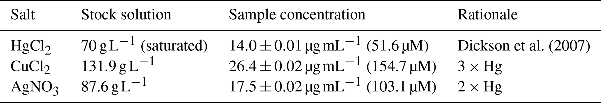
Stock solutions of HgCl2, CuCl2 and AgNO3 were prepared according to Table 1 using high-accuracy chemical equipment (e.g. high-accuracy scale, volumetric flasks). The Ag (silver nitrate EMSURE® ACS; Merck KGaA, Germany) Cu (copper(II) chloride dihydrate; Merck Life Science ApS, Norway) and Hg (mercury(II) chloride; undetermined) salts were dissolved in Milli-Q ultrapure water (> 18 MΩ cm). For measurement of CO2 in seawater samples, the standard method involves poisoning the samples by adding a saturated HgCl2 solution in a volume equal to 0.05 %–0.02 % of the total volume (Dickson et al., 2007). We used this as a starting point and added 0.02 % saturated HgCl2 solution to 18 bottles (240 µL of HgCl2 10× diluted saturated solution), resulting in a sample concentration of 14 µg HgCl2 mL−1 (51.6 µM; Table 1). Based on estimated toxicity relative to Hg (Deheyn et al., 2004; Halmi et al., 2019), the silver and copper salts were added in molar concentrations equal to 2 and 3 times the molar concentration of HgCl2, respectively (Table 1), although this varies between species of microorganisms and environmental matrices (Hassen et al., 1998; Rai et al., 1981).
Table 1Stock and sample concentrations of HgCl2, CuCl2 and AgNO3.
Additional 24 h incubation experiment with different preservatives for pH measurements
Since pH was not measured at the end of the first incubation experiment, we performed an additional experiment to document any potential rapid (within 24 h) impacts of preservative on pH. A total of 48 borosilicate glass bottles (120 mL) filled with lake water were subjected to the same four different treatments as the first experiment described above: HgCl2, CuCl2, AgNO3 or Milli-Q water amendments. To this end, a 20 L water tank was filled with surface water from Lake Svartkulp on 14 December 2023. The water tank was immediately returned to the laboratory and left for 24 h to equilibrate to the room temperature. On 15 December, 120 mL bottles were gently filled with water from the bulk 20 L sample, as described above. The bottles were randomized prior to preservative or Milli-Q treatment performed as described above. The bottles were then incubated at room temperature for 2 or 24 h. The pH was measured in the initial unamended lake water, in 24 bottles opened after 2 h incubation, and in 24 bottles opened after 24 h incubation. The pH measurements were performed with a WTW Multi 3620 pH meter calibrated using a two-point calibration at pH 4 and 7. All pH measures were corrected for temperature. The water temperature of the water samples during pH measurements ranged between 19.1 and 21.2 °C.
2.2 Effects of HgCl2 on dissolved CO2 analyses over a range of pH values
Study site and sampling
Water samples were collected from Lake Lundebyvannet located southeast of Oslo (59.54911° N, 11.47843° E; southeast Norway). Two sets of samples were taken from 1, 1.5, 2 and 2.5 m depth using a water sampler once or twice a week between April 2020 and January 2021 for the determination of (i) dissolved CO2 by gas chromatography (GC) analysis following fixation with HgCl2 and (ii) DIC analysis with a TOC analyser. Samples for GC analysis were filled into 120 mL glass bottles (as described above for the 72 incubation bottles), which were sealed with rubber septa under water without air bubbles. Samples for GC analysis were preserved in the field by adding a half-saturated (at 20 °C) solution of HgCl2 (150 µL) through the rubber seal of each bottle using a syringe, as described above the 72 incubation bottles, resulting in a concentration of 161 µM similar to previous studies (Clayer et al., 2021; Hessen et al., 2017; Yang et al., 2015). Samples for DIC analysis were filled without bubbles in 100 mL Winkler glass bottles that were sealed airtight directly after sampling. These samples were not fixed in any way and were analysed by a TOC analyser within 2 h. Note that estimation of dissolved CO2 concentrations from pH and DIC is the least uncertain method of indirect CO2 concentration with estimated relative error of 6 % or less (Golub et al., 2017). Lake water temperature and pH were measured in situ using HOBO pH data loggers placed at 1, 1.5, 2 and 2.5 m (Elit, Gjerdrum, Norway).
Lake Lundebyvannet has a surface area of 0.4 km2 and a maximum depth of 5.5 m. It often experiences large blooms of Gonyostomum semen over the summer between May and September (Hagman et al., 2015; Rohrlack et al., 2020). The lake water is characterized by high and fluctuating concentrations of humic substances (with DOC concentrations ranging from 8 to 28 mg C L−1), ammonium (5 to 100 µg N L−1), nitrate (20 to 700 µg N L−1), total N (average of 612 µg N L−1), phosphate (2 to 4 µg P L−1), total P (average of 28 µg P L−1; Rohrlack et al., 2020; Hagman et al., 2015), a fluctuating pH (from 5.5 to 7.3), weak ionic strength with alkalinity ranging between 30 and 150 µmol L−1, and electric conductivity varying from 40 to 70 µS cm−1. For more details, see Rohrlack et al. (2020).
Lake Lundebyvannet was selected for this experiment because it is representative of productive, low-ionic-strength Northern Hemisphere lakes typically found in the southern part of granitic bedrock regions in northeast America and Scandinavia.
2.3 Analytical chemistry
Gas chromatography
Headspace was prepared by gently backfilling sample bottles with 20–30 mL helium (He; 99.9999 %) into the closed bottle while removing a corresponding volume of water. Care was taken to control the headspace pressure within 5 % of ambient air, and a slight He overpressure was released before equilibration. The bottles were shaken horizontally at 150 rpm for 1 h to equilibrate gases between the sample and headspace. The temperature during shaking was recorded by a data logger. Immediately after shaking, the bottles were placed in an autosampler (GC-Pal, CTC, Switzerland) coupled to a GC instrument with He back-flushing (model 7890A, Agilent, Santa Clara, CA, USA). Headspace gas was sampled (approx. 2 mL) by a hypodermic needle connected to a peristaltic pump (Gilson MINIPULS 3), which connected the autosampler with the 250 µL heated sampling loop of the GC instrument.
The GC instrument was equipped with a 20 m wide-bore (0.53 mm) PoraPLOT Q column for separation of CH4, CO2 and N2O and a 60 m wide-bore Molsieve 5 Å PLOT column for separation of O2 and N2, both operated at 38 °C and with He as the carrier gas. N2O and CH4 were measured with an electron capture detector run at 375 °C with () as makeup gas and a flame ionization detector, respectively. CO2, O2 and N2 were measured with a thermal conductivity detector (TCD). Certified standards of CO2, N2O and CH4 in He were used for calibration (AGA, Germany), whereas air was used for calibrating O2 and N2. The analytical error for all gases was lower than 2 %. For the Lake Lundebyvannet time series, CO2 was separated from other gases using the 20 m wide-bore (0.53 mm) PoraPLOT Q column, while the other gases were not measured.
The results from gas chromatography give the relative concentration of dissolved gases (in ppm) in the headspace in equilibrium with the water. For the lab experiment with Svartkulp samples (Sect. 2.1), the concentration of dissolved gases in the water at equilibrium with the headspace was calculated from the temperature-corrected Henry constant in water using Carroll et al. (1991) for CO2, Weiss and Price (1980) for N2O, Yamamoto et al. (1976) for CH4, Millero (2002) for O2, and Hamme and Emerson (2004) for N2. For the Lake Lundebyvannet time series (Sect. 2.2), the concentration of CO2 in the water samples was determined using temperature-dependent Henry's law constants given by Wilhelm et al. (1977). The quantities of gases in the headspace and water were summed to find the concentrations and partial pressures of dissolved gases from the water collected in the field as follows:
where [gas] is the gas aqueous concentration, pgas is the gas partial pressure, H is the Henry constant, Vwater is the volume of water sample during headspace equilibration, Vheadspace is the headspace gas volume during equilibration, R is the gas constant and T is the temperature during headspace equilibration (recorded during shaking). The calculations were similar to those of Yang et al. (2015).
DIC analyses
DIC analysis was performed for the Lake Lundebyvannet time series using a Shimadzu TOC-V CPN (Oslo, Norway) instrument equipped with a non-dispersive infrared (NDIR) detector with O2 as a carrier gas at a flow rate of 100 mL min−1. Two to three replicate measurements were run per sample. The system was calibrated using a freshly prepared solution containing different concentrations of NaHCO3 and Na2CO3, and standards were measured in between each sixth sample. CO2 concentrations in water samples ([CO2]) were calculated on the bases of temperature, pH and DIC concentrations as follows (Rohrlack et al., 2020):
where [H+] is the proton concentration (10−pH), CT is the dissolved inorganic carbon concentration and Z is given by
Here K1 and K2 are the first and second carbonic acid dissociation constants adjusted for temperature (pK1=6.41 and pK2=10.33 at 25 °C; Stumm and Morgan, 1996).
2.4 Data analysis
pCO2 and saturation deficit
Lake Lundebyvannet CO2 concentrations provided by GC and DIC analyses were converted to pCO2 (in µatm) as follows:
where KH is the Henry constant for CO2 adjusted for the in situ water temperature (Stumm and Morgan, 1996) and Patm is the atmospheric pressure in bar approximated by
Here altitude is the altitude above sea level of Lake Lundebyvannet (158 m). Finally, the CO2 saturation deficit ( in µatm) was given by
where [CO2]air is the pCO2 in the air (416 µatm for 2020 in southern Norway retrieved from the EBAS database; NILU, 2022; Tørseth et al., 2012). gives the direction of CO2 flux at the water–atmosphere interface, and its product with gas transfer velocity determines the CO2 flux at the water–atmosphere interface, i.e. whether lake ecosystems are sinks () or sources () of atmospheric CO2.
Statistical analyses
The effect of storage time and treatment on five dissolved gases (O2, N2, CO2, CH4, N2O) from the Lake Svartkulp samples was tested with a two-way ANOVA at an alpha level adapted using the Bonferroni correction for multiple testing; i.e. . To evaluate the impact of Hg fixation on Lake Lundebyvannet samples, [CO2] values determined by headspace equilibration and GC analysis of HgCl2-fixed samples were compared with those calculated from DIC measurements of unfixed samples with a paired t test.
A regression analysis was performed to describe the overestimation of CO2 concentrations caused by HgCl2 fixation in Lake Lundebyvannet samples as a function of pH. The total CO2 concentration in the HgCl2-fixed samples () can be expressed as
where [CO2]i is the initial CO2 concentration prior to HgCl2 fixation, i.e. CO2 concentration in the unfixed samples, and [CO2]ex is the excess CO2 concentration caused by a decrease in pH following HgCl2 fixation. The relative CO2 overestimation (E in %) is given by
The impact of pH (or [H+]) on E was mathematically described by running a regression analysis using MATLAB®. The fminsearch MATLAB function from the Optimization Toolbox was used to find the minimum sum of squared residuals (SSR) for functions of the form of or . For each optimal solution, the root-mean-square error (RMSE) and coefficient of determination (R2) were calculated against observed values of E, i.e. values of E determined empirically from observed [CO2]i and [CO2]ex.
Chemical speciation, saturation index calculations and prediction of CO2 overestimation
The speciation of solutes and saturation index (SI) values of selected minerals were calculated with the program PHREEQC developed by the USGS (Parkhurst and Appelo, 2013), neglecting the effect of dissolved organic matter. This was used to assess the impact of the addition of preservative on pH and shifting the carbonate equilibrium as well as dissolved inorganic carbon losses due to carbonate mineral precipitation. PHREEQC is commonly used to calculate the speciation of inorganic carbon and the SI of carbonate minerals and to help estimate the fate of inorganic carbon in carbon-cycling studies (Atekwana et al., 2016; Clayer et al., 2016; Klaus, 2023). For each PHREEQC simulation, two files, the database (with input reactions) and input files, respectively, were used to define the thermodynamic model and the type of calculations to perform. The database of MINTEQA2 (i.e. minteq.dat; Allison et al., 1991) was used to describe the chemical system because it includes, inter alia, reactions and constants for Ag, Cu and Hg complexation with Cl, NO3 and carbonates.
Three PHREEQC simulations were run representing the addition of each preservative solution to sample water from Lake Svartkulp. The input files described the composition of two aqueous solutions: (i) the preservative solution assumed to contain only the preservative (i.e. HgCl2 solution) and (ii) sample water from Lake Svartkulp with observed major element concentrations (pH, Al, Ca, Cl, Cu, Fe, Mg, Mn, N as nitrate, K, Na, S as sulfate, Zn; Table S1) and Hg and Ag natural concentration assumed to be 10−5 mg L−1. The output file provided the activities of the various solutes in the preserved samples, i.e. simulating the mixing of 120 mL of lake water with 240 µL of the AgNO3, CuCl2 and HgCl2 preservative solutions, as described in Sect. 2.1. This procedure allows the estimation of the pH of the preserved samples as well as the SI for various mineral phases. The SI is calculated by PHREEQC comparing the chemical activities of the dissolved ions of a mineral (ion activity product, IAP) with their solubility product (Ks). When SI>1, precipitation is thermodynamically favourable. Note however that PHREEQC does not give information about precipitation kinetics.
Similarly, PHREEQC was used to estimate the decrease in pH caused by adding 150 µL of a half-saturated HgCl2 solution to Lake Lundebyvannet samples prior to GC analyses, as described in Sect. 2.2. In the absence of data on the chemical composition of Lake Lundebyvannet, we assumed that it had the same composition as Lake Svartkulp water samples. This assumption is supported by the fact that waters from both lakes have circumneutral pH, low ionic strength (poor buffering capacity) and high DOC concentration and would therefore behave similarly in the presence of acids. Briefly, for each 0.1 pH value between a pH of 5.4 and 7.3, the carbonate alkalinity was first adjusted by increasing HCO3 concentrations in the input files for PHREEQC to confirm that the water was at equilibrium at the given pH value. Then, the effect of adding 150 µL of a half-saturated HgCl2 solution was simulated as described above for Lake Svartkulp. Knowing the new equilibrated pH, after addition of HgCl2, the overestimation of CO2 concentration in Hg-fixed samples relative to unfixed samples (E, described in Eq. 8 above) can be predicted as described below.
Adapting Eq. (2), we obtain
and
where [H+]i is the proton concentration measured in the initial water samples prior to HgCl2 fixation and is the proton concentration estimated by PHREEQC following HgCl2 fixation, and a similar definition applies for Zi and from Eq. (3). Combining Eqs. (7), (9) and (10), we obtain
Hence
Alternatively, E can also simply be predicted based on the carbonic acid dissociation:
At equilibrium, we have
When pH is decreased upon addition of HgCl2, a fraction (α) of the initial bicarbonate concentration is turned into CO2. This fraction, expressed as [CO2]ex in Eq. (7) above, can be estimated with Eq. (13) as follows:
Introducing the expression of [CO2]ex from Eq. (14) into Eq. (8) yields
When the decrease in pH, or acidification, is greater than the buffering capacity of the water, α=1. The value of α cannot exceed 1 because the amount of CO2 produced by a decrease in pH cannot exceed the amount of initially present. In all the other cases, we have α<1. For both predictions of E, i.e. with Eqs. (12) and (15), the root-mean-square error (RMSE) and coefficient of determination (R2) were calculated.
Finally, additional sources of CO2 overestimation were investigated by analysing the residuals of the model described by Eq. (12), i.e. the difference between E predicted with Eq. (12) and E determined empirically with Eq. (8). Briefly, residuals were plotted against pH and in situ temperature. Residuals were separated into two groups based on the empirical value of ; i.e. the first group had values of , while the second group had values of , where different values for a were used: 20, 10 or 5 µM. The justification for separating residuals into two groups is that (i) the first group represents samples for which bicarbonate alkalinity in the original sample is, as expected, higher than CO2 overestimation after HgCl2 fixation, while (ii) the second group represents samples for which bicarbonate alkalinity is not sufficient to explain CO2 overestimation after HgCl2 fixation.
CO2 diffusion fluxes from Lake Lundebyvannet
The diffusive flux of CO2 ( in ) from Lake Lundebyvannet surface water was estimated according to
where is the CO2 transfer velocity (m d−1), [CO2] is the surface water CO2 concentration (µM), 1000 is a factor to ensure consistency in the units, and [CO2]eq is the theoretical water CO2 concentration (µM) in equilibrium with atmospheric CO2 concentration calculated with Eq. (3) and a pCO2 of 416 µatm (see above).
The CO2 transfer velocity () was estimated as follows (Vachon and Prairie, 2013):
where k600 is the gas transfer velocity (m d−1) estimated from empirical wind-based models and is the CO2 Schmidt number for in situ water temperature (unitless; Wanninkhof, 2014). We used n values of 0.5 or when wind speed was below or above 3.7 m s−1, respectively (Guérin et al., 2007). Empirical k600 models included those from Cole and Caraco (1998; ), Vachon and Prairie (2013; ), and Crusius and Wanninkhof (2003; power model: in cm h−1). U10 and LA refer to mean wind speed at 10 m in m s−1 and lake area in km2, respectively. Sub-hourly U10 data for 2020 were retrieved from a weather station of the Norwegian Meteorological Institute located 1.5 km west of Lake Lundebyvannet (station name: E18 Melleby; ID: SN 3480; 59.546° N, 11.4535° E) using the Frost application programming interface (Frost API, 2022). Daily, monthly and yearly (only covering the ice-free season: April–November) was estimated using Eq. (12). Daily [CO2] was interpolated from weekly data using a modified Akima spline (makima spline in MATLAB® based on Akima, 1974). This interpolation method is known to avoid excessive local undulations.
3.1 Effects of preservatives and storage time on dissolved gases
In the unfixed samples from Lake Svartkulp, the concentration of O2 declined while CO2 increased over time in a close to 1:1 molar ratio, likely reflecting the effect of microbial respiration activity and mineralization of organic matter (Fig. 2 and Table S2 in the Supplement). The concentration of O2 in the unfixed samples decreased from near 300 to below 200 µM (Fig. 2). In the presence of inhibitors, O2 concentrations tended to be slightly higher at t=24 h and remained constant or declined only slightly over time to generally remain at or above saturation (280 to 300 µM). Thus, the inhibitors were effective in reducing oxic respiration.
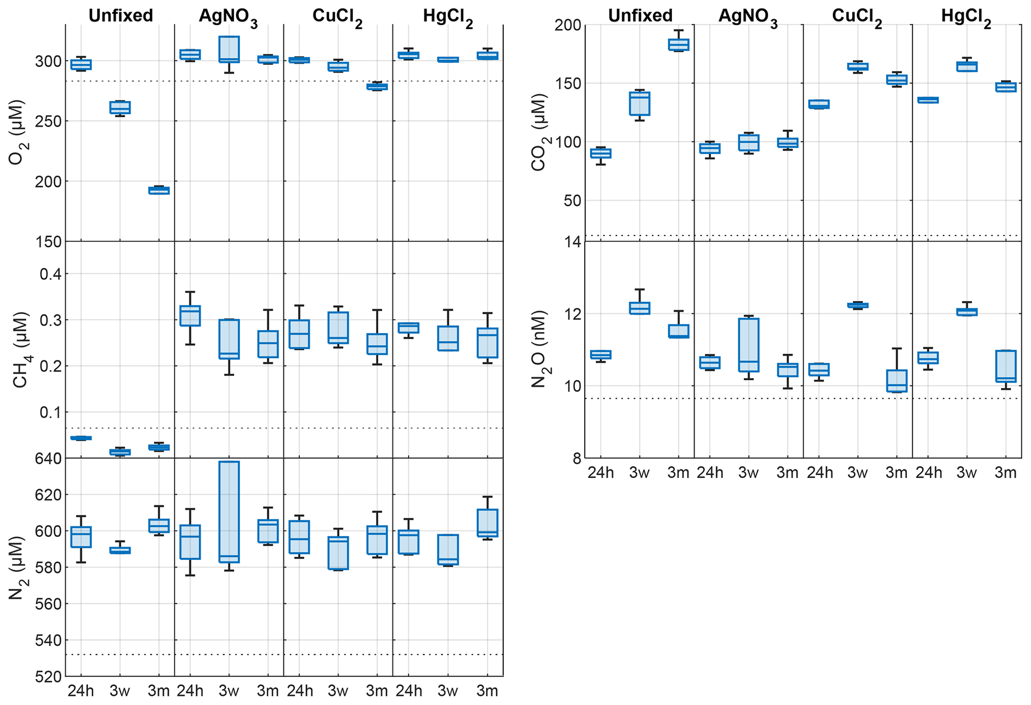
Figure 2Changes in dissolved O2, CO2, CH4, N2O and N2 concentrations (nM or µM) in the absence (unfixed) and presence of different preservatives (AgNO3, CuCl2, HgCl2) at three different times (24h, 24 h after incubation start; 3w, 3 weeks after collection; 3m, 3 months after collection). The horizontal dotted line is the saturated gas concentration corresponding to 100 % gas saturation at in situ lake temperature. Box plots show the median and 25th and 75th percentiles, and the whiskers display the minimum and maximum.
The concentration of CO2 in the presence of AgNO3 at t=24 h was not significantly different to the unfixed at t=0 (Fig. 2; paired t test, P>0.1). At t=24 h, CO2 concentrations were however much higher in the presence of HgCl2 (135 µM) or CuCl2 (131 µM) than in the unfixed (89 µM; Fig. 2 and Table S2). The CO2 further increases from 130 to ∼ 160 µM after 3 weeks in both sample sets preserved with HgCl2 and CuCl2, while a decrease in O2 is less pronounced for samples fixed with CuCl2 and completely absent for samples fixed with HgCl2. Overall, the addition of HgCl2 or CuCl2 following sampling increased CO2 concentrations by 47 % after 24 h compared to the unfixed and caused further changes over the 3-month storage time, while preservation with AgNO3 yielded CO2 concentrations consistent with the unfixed and caused negligible changes over time (Fig. 2; paired t test, P>0.1).
The concentration of CH4 across all samples ranged between 0.017 and 0.377 µM (Fig. 2), as expected 2 orders of magnitude smaller than CO2. At t=24 h, the concentration of CH4 was over 0.2 µM in the presence of inhibitors, while it was below saturation in the unfixed (0.03 µM; Fig. 2). CH4 oversaturation in the preserved samples persisted after 3 weeks and 3 months of storage, and CH4 concentration remained unchanged (Fig. 2 and Table S2).
The concentration of N2O ranged between 9.8 and 12.7 nM with only samples preserved with AgNO3 showing negligible changes over time (Fig. 2; paired t test, P>0.1). All the other samples showed consistent patterns with storage time. N2O concentrations initially increased within the first 3 weeks, followed by a decrease after 3 months.
The changes in N2 were likely within handling and analytical errors and not different in the presence or absence of inhibitors (Fig. 2 and Table S2; paired t test, P>0.1).
3.2 Effects of preservatives on pH
In the samples amended with ultrapure water or AgNO3, the pH did not show any significant changes after 2 or 24 h. In contrast, both groups with HgCl2 and CuCl2 treatments show significant decreases in pH after 2 h, −0.12 and −0.19, respectively, and 24 h, −0.16 and −0.21, respectively. In addition, they showed a significant decrease in pH from 2 to 24 h. Samples amended with CuCl2 show the strongest decrease in pH.
3.3 Contrasting impacts of HgCl2, CuCl2 and AgNO3 on dissolved CO2 estimation revealed by chemical speciation modelling
The PHREEQC simulation of unpreserved samples, based on concentrations of all major elements (Table S1), predicted a pH of 6.72 (Table 2), which is very close to the measured pH of 6.73 (Table S1). This suggests that chemical information provided to PHREEQC is likely sufficient to describe the system, without having to invoke more complex reactions with dissolved organic matter. The addition of HgCl2 and CuCl2 both caused a significant decrease in pH to 6.40 and 6.45, respectively (Table 2), which is similar to the decrease observed at the end of the 24 h short-term incubation (Fig. 3).
Table 2The pH and saturation indices of selected carbonate minerals estimated by PHREEQC for the unpreserved and preserved samples.
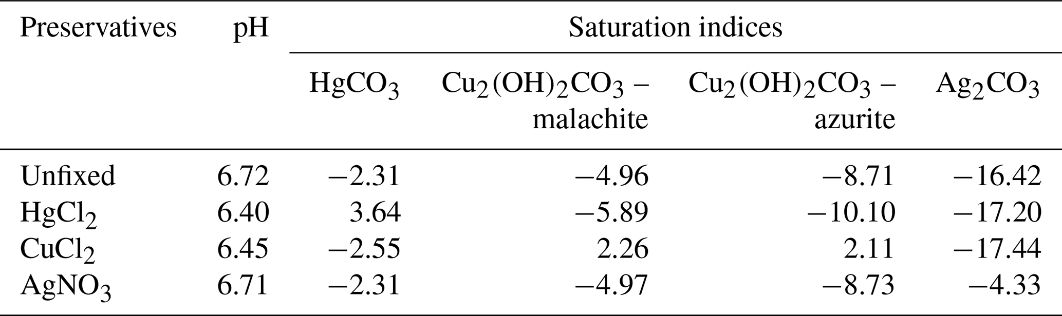
In the absence of preservatives, none of the common carbonate minerals, including calcite, were associated with a saturation index higher than 1; i.e. dissolution was thermodynamically favourable for all these minerals and no DIC loss was expected (Table 2). However, upon addition of HgCl2 or CuCl2, some carbonate minerals, e.g. HgCO3 or malachite and azurite, respectively, were expected to spontaneously precipitate given their relatively high saturation index values.
3.4 Effects of HgCl2 on dissolved CO2 concentration under a range of pH values
CO2 concentrations in unfixed water samples from Lake Lundebyvannet were significantly lower than in the HgCl2-fixed samples (mean difference: 52 µM; paired t test; P<0.0001; Table 3). Fixation with HgCl2 caused a general overestimation of CO2 concentration and the saturation deficit (Fig. 4), thus missing out events of CO2 influx (carbon sink) under conditions of high photosynthesis activity (high pH; Fig. 4). In parallel, PHREEQC predicted a decrease of 0.6 to 1.8 units of pH related to HgCl2 addition (Fig. S1 in the Supplement).
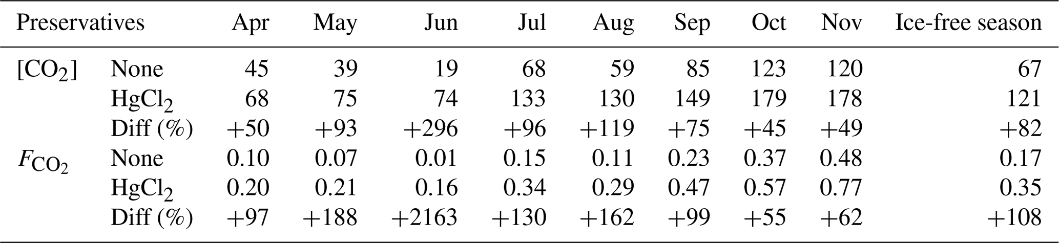
Table 3CO2 concentrations ([CO2], µM) and diffusion fluxes (, ) from Lake Lundebyvannet estimated from HgCl2-fixed and unfixed samples following Cole and Caraco (1998). The ice-free season spans April to November. Data are also shown in Fig. 6.
The pH value of water samples from Lake Lundebyvannet varied between 5.4 and 7.3 (Figs. 4 and 5), mainly due to marked variations in phytoplankton photosynthetic activity (Rohrlack et al., 2020). The relative overestimation of CO2 (E) follows an exponential increase with pH and is well reproduced by a simple exponential function (, RMSE=44 %, R2=0.81, p<0.0001; Fig. 5).
Prior to using dissolved gas concentrations in freshwater to estimate the magnitude of biological aquatic processes such as photosynthesis and oxic respiration, denitrification, and methanogenesis, we must ensure that biological activity between sampling and laboratory analyses was efficiently inhibited without significant impacts on the sample's chemistry. Here we report a unique dataset on the impact of three preservatives on water samples from a typical low-ionic-strength, unproductive boreal lake to give information on potential risks of misestimation of dissolved gas concentrations. We further show, using CO2 concentration data from a typical productive boreal lake, that using HgCl2 can lead to negligence of the role of photosynthesis in lake C cycling.
4.1 Best preservative for the determination of dissolved gas concentrations
Given that none of the four treatments (unfixed, HgCl2, CuCl2 or AgNO3) applied to Lake Svartkulp water samples during the 3-month incubation offer an independent control, a first challenge is to determine which of the treatments represent the most realistic dissolved gas concentrations close to real conditions. For CO2 and O2, a few studies have used unfixed samples (only preserved dark at +4 °C) up to 48 h after sampling to determine CO2 or DIC concentrations (e.g. Sobek et al., 2003; Kokic et al., 2015). Therefore, the CO2 and O2 concentrations in the unfixed samples collected after 24 h incubation are the most representative of the initial real concentrations. Biological activity might have had an impact, but this is likely negligible over the first 24 h. In addition, the fact that the CO2 and O2 concentrations in the samples fixed with AgNO3 after 24 h, 3 weeks and 3 months are equal to those from unfixed samples after 24 h (Fig. 2) confirms that the unfixed samples after 24 h can be used as a control. In fact, only samples fixed with AgNO3 are reliable given the expected toxicity of Ag, the absence of an impact on pH (Fig. 3) and unchanged concentrations over the 3-month experiment for all gases. Similarly, N2O and N2 concentrations in the unfixed samples after 24 h can be used as a control. However, for CH4, Fig. 2 shows that after only 24 h, the CH4 concentration in the unfixed samples is below atmospheric saturation while it is consistently much higher in all three sets of fixed samples. Boreal lakes are typically oversaturated with respect to CH4 (Valiente et al., 2022), and it is very unlikely that CH4 could have been produced in lake water incubated under high concentrations of oxygen and toxic preservatives. Hence, unfixed samples do not represent real CH4 concentrations. These observations are all consistent with the fact that the three preservatives were effective in preserving CH4 from oxidation. Even over 24 h, preservatives need to be added to oxic water samples to preserve CH4 from oxidation. In fact, oxic methanotrophy typically shows rates on the order of µM d−1 (Thottathil et al., 2019; van Grinsven et al., 2021). Hence, a CH4 consumption of 0.3 µM within 24 h in the unfixed water samples is realistic (Fig. 2).
In summary, preservation with AgNO3 is the only method that offered robust determination of all five dissolved gases with negligible changes in concentration over time.

Figure 3Observed changes in pH in the absence (unfixed) and presence of different preservatives (AgNO3, CuCl2, HgCl2) at two different times, 2 and 24 h after the start of the incubation. The horizontal dotted line represents the initial pH of the bulk water sample. Box plots show the median and 25th and 75th percentiles, and the whiskers display the minimum and maximum of the six replicates. Stars indicate groups that are significantly different from each other and from the initial pH (two-way ANOVA).

Figure 4CO2 saturation deficit () in Lake Lundebyvannet as a function of in situ pH for all unfixed (obtained from DIC analysis) and HgCl2-fixed (obtained from GC analysis) samples (a). Time series of the pH and CO2 saturation deficit of surface water (1 m deep) for unfixed and HgCl2-fixed samples (b).

Figure 5Comparison of observed (circles) and predicted (blue line) relative overestimation (E) of CO2 concentrations caused by HgCl2 fixation in Lake Lundebyvannet samples as a function of pH (a) or proton concentration (b). The black line shows the best fit of the regression analysis. Yellow symbols represent samples for which the bicarbonate concentration in the unfixed samples () is nearly equal to CO2 overestimation ([CO2]ex), i.e. ±20 µM (equivalent to a pH error of 0.05), while red and blue symbols represent samples for which initial bicarbonate concentration was lower and higher, respectively, than the CO2 overestimation.
4.2 Risks of misestimating dissolved gas concentration with HgCl2 and CuCl2 preservation
Both sets of samples preserved with either HgCl2 or CuCl2 showed CO2 concentrations that were much higher than the unfixed (after 24 h) or the AgNO3-fixed samples. This is due to an acidification of the poorly buffered (alkalinity 127 µM) and near-neutral water (pH=6.73), shifting the carbonate equilibrium from HCO3 to CO2 as also shown by Borges et al. (2019). In fact, a rapid decrease in pH was observed upon HgCl2 and CuCl2 treatments (Fig. 3). The increase in CO2 from about 130 to ∼ 160 µM after 3 weeks in both sample sets preserved with HgCl2 and CuCl2 is not mirrored by a similar decrease in O2 (Fig. 2). This suggests that oxic respiration is not the main source for this additional 30 µM of CO2 but rather points towards additional acidification of the samples caused, for example, by kinetically controlled complexation of Hg2+ with dissolved organic matter (Miller et al., 2009). In fact, the relatively slow complexation of Hg2+ with organic thiol groups can release two protons (Skyllberg, 2008) and up to three, with some participation of a third weak-acid group (Khwaja et al., 2006). The transient nature of acidification caused by HgCl2 and CuCl2 is also evident in the pH impacts showing higher acidification after 24 h than after 2 h incubation (Fig. 3). The following decrease in CO2 after 3 months (down to ∼ 145 µM) points to other processes. The precipitation of Hg and Cu carbonates, given their high saturation index values (Table 2), would be consistent with the decrease in CO2 concentrations observed between 3 weeks and 3 months. Calcite precipitation is typically observed in supersaturated solutions within 48 h (Kim et al., 2020). Hence, it is realistic to assume that Hg and Cu carbonate precipitation influenced the CO2 concentration within the preserved samples over the 3 months of storage time. Impacts of Hg or Cu carbonate precipitation are not evident after 3 weeks, likely because of slow but persistent CO2 production in the presence of HgCl2 and CuCl2 related to acidification as described above (Fig. 2). However, after 3 weeks, this production likely weakens and is counterbalanced by increasing carbonate precipitation.
Overall, the addition of HgCl2 or CuCl2 following sampling increased CO2 concentrations by 47 % within the first 24 h compared to the unfixed, consistent with the acidification of −0.16 to −0.21 pH units observed over the same time in the pH incubation experiment (Fig. 3) and the pH estimated with PHREEQC without the interaction with dissolved organic matter (Table 2). In fact, introducing pH and CO2 concentration values of 6.40–6.45 and 130 µM, respectively, for the samples preserved with HgCl2 and CuCl2 into Eqs. (1) and (2) yields DIC concentrations (CT) of about 270 µM at t=24 h. These DIC concentrations are almost equal to those calculated for the unfixed samples and those preserved with AgNO3 at t=24 h, i.e. with a pH of 6.73 and CO2 concentration of 88 µM. Interestingly, the concentration of CO2 in the samples preserved with HgCl2 and CuCl2 continues to increase up to ∼ 160 µM after 3 weeks. Given that oxic respiration is inhibited (Fig. 2), this additional CO2 is believed to originate from the progressive release of protons following the relatively slow complexation of Hg2+ with dissolved organic matter (Khwaja et al., 2006; Miller et al., 2009; Skyllberg, 2008). Note however that this process could not be predicted with PHREEQC given that it neglected the effect of dissolved organic matter.
Unlike the AgNO3-fixed samples, all the other samples showed an initial increase in N2O concentration from 24 h to 3 weeks, followed by a decrease from 3 weeks to 3 months. Similar patterns of net N2O production followed by net consumption were also reported in short-term incubations of seawater from the high-latitude Atlantic Ocean, although over much shorter timescales, i.e. 48 and 96 h (Rees et al., 2021). The large difference in kinetics between the latter experiment (Rees et al., 2021) and our incubation might be attributable to differences in incubation temperature, where the seawater from the high-latitude Atlantic Ocean was incubated at ambient temperatures while our samples were kept at +4 °C. Other differences in the experimental setup might have also played a role. The lack of inhibition of N2O production and consumption in the samples preserved with HgCl2 and CuCl2 can be attributed to the fact that N2O production tends to increase under increasing acidic conditions (Knowles, 1982; Mørkved et al., 2007; Seitzinger, 1988). In fact, the mole fraction of N2O produced during denitrification increases compared to N2 as pH decreases (Knowles, 1982).
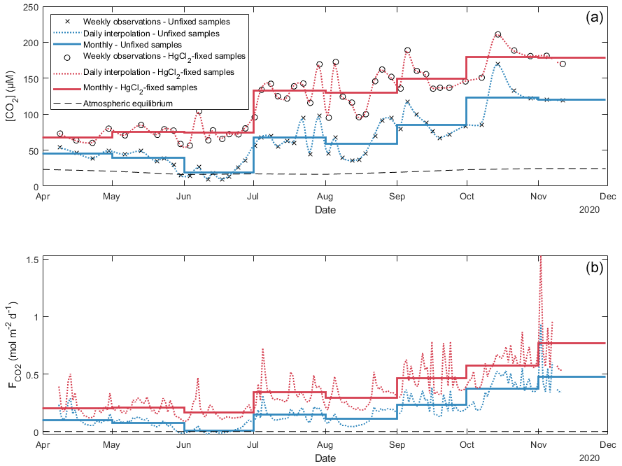
Figure 6Daily and monthly surface CO2 concentrations ([CO2]; a) and diffusion fluxes (; b) at the water–atmosphere interface from Lake Lundebyvannet (also in Table 3). Unfixed samples were obtained by DIC analysis. Daily [CO2] was interpolated from weekly data using a modified spline (see text for details). Diffusion fluxes were calculated following Cole and Caraco (1998).
4.3 Using PHREEQC to estimate acidification caused by HgCl2 in samples from Lake Lundebyvannet
As for the samples from Lake Svartkulp as described above, the overestimation of CO2 concentration in the samples from Lake Lundebyvannet fixed with HgCl2 (161 µM added; Fig. 4) likely stems from the acidification shifting the carbonate equilibrium from bicarbonate to CO2. In fact, PHREEQC predicted a decrease of 0.6 to 1.8 units of pH related to HgCl2 addition in these samples (Fig. S1).
The relative overestimation of CO2 (E in Fig. 5) followed a typical exponential increase reflecting the decrease in absolute CO2 concentration with increasing pH (Stumm and Morgan, 1981), caused here by phytoplankton photosynthesis. In fact, the exponential increase in CO2 overestimation is easily predicted by Eq. (9) with an equivalent level of accuracy to the optimized exponential function (Fig. 5). Consistently, the relative overestimation of CO2 (E) shows an inverse decrease with [H+] that is well reproduced by a simple inverse function (; RMSE=44 %, R2=0.81, p<0.0001; Fig. 5) and predicted by Eq. (15), with an α value of 1. Combining Eqs. (8) and (15) and solving this with pH values estimated from PHREEQC (Fig. S1) for α yields values ranging between 0.72 and 0.89 with an average of 0.85. Unexpectedly, this average α value is almost equal to the ratio of the inverse function coefficient and K1; i.e. . Hence, the relative overestimation of CO2 (E) caused by HgCl2 fixation is easily predicted by the change in bicarbonate equilibrium knowing the proton release from HgCl2 addition, here estimated with PHREEQC.
Hence, PHREEQC can be used to predict a decrease in pH caused by HgCl2 fixation if sufficient knowledge is gathered on the ionic water composition. Proton release during HgCl2 fixation can be represented by the following reaction:
From Reaction (R2), it becomes evident that the initial concentration of chloride in the water samples will likely limit HgCl2 dissociation and proton release. This is a mechanism that is likely to occur in seawater where HgCl2 has been shown to cause a decrease in pH, although at a negligible level with a maximum decrease in pH of −0.01 (Chou et al., 2016).
Figure 5 shows that a range of water samples were associated with a relative CO2 overestimation (E) that substantially deviated from the overestimation predicted with Eq. (12) (red and blue symbols in Fig. 5). In fact, some samples had a higher initial bicarbonate content () than the excess CO2 concentration ([CO2]ex), while others showed the opposite. The former case (blue symbols in Fig. 5) can easily be explained by a higher buffering capacity of the sampled water, i.e. a higher pH after HgCl2 fixation than that predicted by PHREEQC related to a different water composition. Indeed, the concentration of major elements in the water from Lake Lundebyvannet may vary significantly over time, and in the absence of data, we considered that the water composition, except for DIC, pH and HgCl2, was constant over time. By contrast, samples associated with [CO2]ex being larger than are more enigmatic. In order to shed light on possible explanations, we visually inspected trends between empirical deviations from predictions, i.e. residuals, and in situ temperature or pH. Absolute values of residuals showed a progressive increase with pH and in situ temperature, which is in agreement with decreasing precision of the headspace method with increasing temperature and pH (Koschorreck et al., 2021). In fact, CO2 is less soluble at higher temperature; hence there can be more gas evasion during sampling, and thus the error increases with in situ temperature. In addition, at higher pH, CO2 concentration decreases, and consequently the absolute error in CO2 quantification becomes larger relative to measured CO2 concentration. Interestingly, many of the high residual values were not evenly distributed across the year or across the summer and instead were associated with only a few specific sampling events during summer (Fig. S2 in the Supplement). This suggests that degassing could have occurred due to high ambient temperature in the field. Water associated with [CO2]ex being larger than (red symbols in Figs. 5 and S4 in the Supplement) could have been subject to larger degassing in the samples collected for DIC analysis than the samples for GC analysis. On the other hand, degassing was likely larger for samples for GC analysis than for DIC analysis for water associated with being larger than [CO2]ex (blue symbols in Figs. 5 and S2). In addition to degassing and temperature effects, errors in pH measurements can also cause a large misestimation of CO2 concentration from DIC analysis, and this error increases exponentially with pH following the shift in the carbonate equilibrium. In summary, our analysis is consistent with that of Koschorreck et al. (2021), showing that errors in the determination of CO2 concentrations are smaller at lower pH values and lower temperature (Fig. S2).
4.4 Implications for the estimation of lake and reservoir C cycling and recommendations
Using HgCl2 or CuCl2 to preserve dissolved gas samples in poorly buffered water samples has large impacts on CO2 concentrations with considerable risk of leading to incorrect interpretations. The risk of misestimating CO2 concentration due to HgCl2 and CuCl2 preservation is the highest when the pH of the unfixed water is close to the first carbonic acid dissociation constant (pK1=6.41 at 25 °C; Stumm and Morgan, 1996). This implies that any small shift in pH will have a significant impact on the carbonate equilibrium between bicarbonate and CO2. The risk is also the highest in the lowest-ionic-strength waters. In that respect, low-ionic-strength, slightly acidic to neutral, moderately humic lakes commonly found in Norway (de Wit et al., 2023); large parts of Sweden (Valinia et al., 2014); Finland and Atlantic Canada (Houle et al., 2022); and Ontario, Quebec and northeast USA (Skjelkvåle and de Wit, 2011; Weyhenmeyer et al., 2019) are the most prone to errors in CO2 concentrations related to HgCl2 or CuCl2 preservation. Through a preliminary literature search, we found several studies not only from boreal lakes (Jonsson et al., 2001; Urabe et al., 2011; Yang et al., 2015; Hessen et al., 2017) but also from circumneutral-pH sub-tropical to tropical aquatic environments (Jeffrey et al., 2018; Webb et al., 2018; Ray et al., 2021) where preservation with HgCl2 may have caused biases in the quantification of CO2 concentrations as was the case for samples from the Congo River (Borges et al., 2019). A significant part of the low-ionic-strength boreal lakes are becoming increasingly sensitive to changes in nutrients with strong impacts on their role in carbon cycling (Myrstener et al., 2022). In this context, it is crucial to avoid misestimation of CO2 concentrations and thus avoid use of HgCl2 or CuCl2 to ensure a robust understanding of the role of autotrophic processes in lake C cycling. Below we describe the implications for the lake C budget of Lundebyvannet as an example of a misestimation of the role of photosynthesis in a typical productive boreal lake.
In Lake Lundebyvannet, over the ice-free season, average CO2 concentrations determined following HgCl2 fixation and GC analysis were 82 % higher than those obtained from DIC analyses (Table 3; Figs. 6 and S3 in the Supplement). CO2 concentrations obtained from HgCl2-fixed samples created the illusion that Lake Lundebyvannet was a steady net source of CO2 to the atmosphere over the ice-free season with a large CO2 saturation deficit (Fig. 4), while, in reality, the lake switched from being a net source in May to a net sink over a few weeks in Jun, and to a net source again in July (Figs. 6 and S3). Indeed, monthly CO2 overestimation related to HgCl2 fixation reached about 300 % in June (Table 3). Propagating this overestimation into the estimates of CO2 diffusion fluxes with typical wind-based models yields an overestimation of CO2 fluxes of 108 %–112 % over the ice-free season and up to 2100 % in June (Tables 3 and S3 in the Supplement). Hence, interpreting CO2 data without correcting for CO2 overestimation caused by HgCl2 fixation leads to negligence of the role of photosynthesis in lake C cycling, with major implications for current and future predictions of lake CO2 emissions.
The use of HgCl2 to preserve water samples prior to dissolved gas analyses is part of current guidelines for greenhouse gas measurements in freshwater reservoirs (Machado Damazio et al., 2012; UNESCO/IHA, 2008, 2010). Hence, there is a risk of overestimating CO2 concentrations and emissions, in the absence of the discrete measurement of emissions, from hydropower reservoirs, with consequences for the present and expected greenhouse gas footprint from hydroelectricity. To ensure precise estimation of greenhouse gas concentration and, possibly, emission from hydropower, the use of HgCl2 should therefore be discontinued.
Mercury is a potent neurotoxin for humans and toxic for the environment, and its use should be discouraged, notably following the Minamata Convention on Mercury, a global treaty ratified by 126 countries (16 December 2020) to protect human health and the environment from the adverse effects of mercury. This study further questions the use of HgCl2 for preservation of poorly buffered (low-ionic-strength) water samples with high DOC concentration for analysis of dissolved gases in the laboratory. Although CuCl2 is less toxic, it behaved similarly to HgCl2 and cannot be recommended. In fact, both chlorinated inhibitors caused a significant decrease in pH, shifting the carbonate equilibrium towards CO2, and are also suspected to promote carbonate precipitation over long-term storage. The only promising inhibitor tested in this study was AgNO3, notably for dissolved CO2, CH4 and N2O. Silver nitrate is a suitable substitute for HgCl2 in low-ionic-strength waters; further tests should be carried out with a range of inhibitor concentration and more diverse water samples. The use of chemical inhibitors may not be the best approach. Alternatives exist, such as directly measuring gas concentrations in situ with sensors; sampling the headspace out in the field; and bringing back gas samples (e.g. Cole et al., 1994; Karlsson et al., 2013; Kling et al., 1991; Valiente et al., 2022), rather than water samples, to the lab for gas chromatography analyses. However, care must be taken to know the exact equilibration temperature (Koschorreck et al., 2021) and to avoid gas exchange with the atmosphere as well as to use a clean background gas during headspace equilibration, which can be challenging in remote environments under harsh meteorological conditions.
We further advise against interpretation of CO2 concentration data from low-ionic-strength, circumneutral water samples preserved with HgCl2 or CuCl2. The overestimation of CO2 concentration caused by HgCl2 can mask the effect of photosynthesis on lake carbon balance, creating the illusion that lakes are net CO2 sources when they are net CO2 sinks. Our analysis from Lake Lundebyvannet shows that HgCl2 fixation led to an overestimation of the CO2 concentration by a factor of 1.8, on average, but approaching a factor of 4 during the peak photosynthetic period. An even larger impact is expected on CO2 diffusive fluxes, which were overestimated by a factor of 2 on average and up to a factor of > 20 during peak photosynthesis. Interpreting such data would have underestimated the current and future role of aquatic photosynthesis.
All data supporting this study are available at https://doi.org/10.4211/hs.436be40748a246269102b20211b49762 (Clayer et al., 2024).
The supplement related to this article is available online at: https://doi.org/10.5194/bg-21-1903-2024-supplement.
JET, AK and TR supervised and PD, KN and FC contributed to the study design. JET, KN and TR carried out the experiments. PD and TR performed the chemical analyses. JET and FC wrote the first draft. FC performed the modelling and data and statistical analyses and drafted the figures. All co-authors edited the manuscript.
The contact author has declared that none of the authors has any competing interests.
Publisher's note: Copernicus Publications remains neutral with regard to jurisdictional claims made in the text, published maps, institutional affiliations, or any other geographical representation in this paper. While Copernicus Publications makes every effort to include appropriate place names, the final responsibility lies with the authors.
We are grateful to Benoît Demars for research assistance, coordination, and useful comments and discussions on an earlier version of this paper and to Heleen de Wit for discussions. Research was funded by NIVA and through the Global Change at Northern Latitude (NoLa) project.
This research has been supported by the Norsk Institutt for Vannforskning (grant no. 200033).
This paper was edited by Tyler Cyronak and reviewed by Judith Vogt and Sigrid van Grinsven.
Akima, H.: A method of bivariate interpolation and smooth surface fitting based on local procedures, Commun. ACM, 17, 18–20, https://doi.org/10.1145/360767.360779, 1974.
Allison, J., Brown, D., and Novo-Gradac, K.: MINTEQA2/PRODEFA2, a geochemical assessment model for environmental systems: Version 3. 0 user's manual, US Environmental Protection Agency, GA, PB-91-182469/XAB; EPA-600/3-91/021, https://www.osti.gov/biblio/5673069 (last access: 15 April 2024), 1991.
Amorim, M. J. B. and Scott-Fordsmand, J. J.: Toxicity of copper nanoparticles and CuCl2 salt to Enchytraeus albidus worms: Survival, reproduction and avoidance responses, Environ. Pollut., 164, 164–168, https://doi.org/10.1016/j.envpol.2012.01.015, 2012.
Atekwana, E. A., Molwalefhe, L., Kgaodi, O., and Cruse, A. M.: Effect of evapotranspiration on dissolved inorganic carbon and stable carbon isotopic evolution in rivers in semi-arid climates: The Okavango Delta in North West Botswana, J. Hydrol. Reg. Stud., 7, 1–13, https://doi.org/10.1016/j.ejrh.2016.05.003, 2016.
Borges, A. V., Darchambeau, F., Lambert, T., Morana, C., Allen, G. H., Tambwe, E., Toengaho Sembaito, A., Mambo, T., Nlandu Wabakhangazi, J., Descy, J.-P., Teodoru, C. R., and Bouillon, S.: Variations in dissolved greenhouse gases (CO2, CH4, N2O) in the Congo River network overwhelmingly driven by fluvial-wetland connectivity, Biogeosciences, 16, 3801–3834, https://doi.org/10.5194/bg-16-3801-2019, 2019.
Carroll, J. J., Slupsky, J. D., and Mather, A. E.: The Solubility of Carbon Dioxide in Water at Low Pressure, J. Phys. Chem. Ref. Data, 20, 1201–1209, https://doi.org/10.1063/1.555900, 1991.
Chen, C. Y., Driscoll, C. T., Eagles-Smith, C. A., Eckley, C. S., Gay, D. A., Hsu-Kim, H., Keane, S. E., Kirk, J. L., Mason, R. P., Obrist, D., Selin, H., Selin, N. E., and Thompson, M. R.: A Critical Time for Mercury Science to Inform Global Policy, Environ. Sci. Technol., 52, 9556–9561, https://doi.org/10.1021/acs.est.8b02286, 2018.
Chen, H., Johnston, R. C., Mann, B. F., Chu, R. K., Tolic, N., Parks, J. M., and Gu, B.: Identification of Mercury and Dissolved Organic Matter Complexes Using Ultrahigh Resolution Mass Spectrometry, Environ. Sci. Tech. Let., 4, 59–65, https://doi.org/10.1021/acs.estlett.6b00460, 2017.
Chou, W.-C., Gong, G.-C., Yang, C.-Y., and Chuang, K.-Y.: A comparison between field and laboratory pH measurements for seawater on the East China Sea shelf, Limnol. Oceanogr.-Meth., 14, 315–322, https://doi.org/10.1002/lom3.10091, 2016.
Ciavatta, L. and Grimaldi, M.: The hydrolysis of mercury(II) chloride, HgCl2, J. Inorg. Nucl. Chem., 30, 563–581, https://doi.org/10.1016/0022-1902(68)80483-X, 1968.
Clayer, F., Gobeil, C., and Tessier, A.: Rates and pathways of sedimentary organic matter mineralization in two basins of a boreal lake: Emphasis on methanogenesis and methanotrophy: Methane cycling in boreal lake sediments, Limnol. Oceanogr., 61, S131–S149, https://doi.org/10.1002/lno.10323, 2016.
Clayer, F., Thrane, J.-E., Brandt, U., Dörsch, P., and de Wit, H. A.: Boreal Headwater Catchment as Hot Spot of Carbon Processing From Headwater to Fjord, J. Geophys. Res.-Biogeo., 126, e2021JG006359, https://doi.org/10.1029/2021JG006359, 2021.
Clayer, F., Thrane, J.-E., Dörsch, P., and Rohrlack, T.: Dataset for “Technical Note: Preventing CO2 overestimation from mercuric or copper (II) chloride preservation of dissolved greenhouse gases in freshwater samples”, https://doi.org/10.4211/hs.436be40748a246269102b20211b49762, 2024.
Cole, J. J. and Caraco, N. F.: Atmospheric exchange of carbon dioxide in a low-wind oligotrophic lake measured by the addition of SF6, Limnol. Oceanogr., 43, 647–656, https://doi.org/10.4319/lo.1998.43.4.0647, 1998.
Cole, J. J., Caraco, N. F., Kling, G. W., and Kratz, T. K.: Carbon Dioxide Supersaturation in the Surface Waters of Lakes, Science, 265, 1568–1570, https://doi.org/10.1126/science.265.5178.1568, 1994.
Crusius, J. and Wanninkhof, R.: Gas transfer velocities measured at low wind speed over a lake, Limnol. Oceanogr., 48, 1010–1017, https://doi.org/10.4319/lo.2003.48.3.1010, 2003.
de Wit, H. A., Garmo, Ø. A., Jackson-Blake, L. A., Clayer, F., Vogt, R. D., Austnes, K., Kaste, Ø., Gundersen, C. B., Guerrerro, J. L., and Hindar, A.: Changing Water Chemistry in One Thousand Norwegian Lakes During Three Decades of Cleaner Air and Climate Change, Global Biogeochem. Cy., 37, e2022GB007509, https://doi.org/10.1029/2022GB007509, 2023.
Deheyn, D. D., Bencheikh-Latmani, R., and Latz, M. I.: Chemical speciation and toxicity of metals assessed by three bioluminescence-based assays using marine organisms, Environ. Toxicol., 19, 161–178, https://doi.org/10.1002/tox.20009, 2004.
Dickson, A. G., Sabine, C. L., and Christian, J. R.: Guide to best practices for ocean CO2 measurements, North Pacific Marine Science Organization, https://doi.org/10.25607/OBP-1342, 2007.
Duan, Z. and Mao, S.: A thermodynamic model for calculating methane solubility, density and gas phase composition of methane-bearing aqueous fluids from 273 to 523 K and from 1 to 2000 bar, Geochim. Cosmochim. Ac., 70, 3369–3386, https://doi.org/10.1016/j.gca.2006.03.018, 2006.
Foti, C., Giuffrè, O., Lando, G., and Sammartano, S.: Interaction of Inorganic Mercury(II) with Polyamines, Polycarboxylates, and Amino Acids, J. Chem. Eng. Data, 54, 893–903, https://doi.org/10.1021/je800685c, 2009.
Frost API: https://frost.met.no/index.html (last access: 15 April 2024), 2022.
Golub, M., Desai, A. R., McKinley, G. A., Remucal, C. K., and Stanley, E. H.: Large Uncertainty in Estimating pCO2 From Carbonate Equilibria in Lakes, J. Geophys. Res.-Biogeo., 122, 2909–2924, https://doi.org/10.1002/2017JG003794, 2017.
Guérin, F., Abril, G., Richard, S., Burban, B., Reynouard, C., Seyler, P., and Delmas, R.: Methane and carbon dioxide emissions from tropical reservoirs: Significance of downstream rivers, Geophys. Res. Lett., 33, L21407, https://doi.org/10.1029/2006GL027929, 2006.
Guérin, F., Abril, G., Serça, D., Delon, C., Richard, S., Delmas, R., Tremblay, A., and Varfalvy, L.: Gas transfer velocities of CO2 and CH4 in a tropical reservoir and its river downstream, J. Marine Syst., 66, 161–172, https://doi.org/10.1016/j.jmarsys.2006.03.019, 2007.
Hagman, C. H. C., Ballot, A., Hjermann, D. Ø., Skjelbred, B., Brettum, P., and Ptacnik, R.: The occurrence and spread of Gonyostomum semen (Ehr.) Diesing (Raphidophyceae) in Norwegian lakes, Hydrobiologia, 744, 1–14, https://doi.org/10.1007/s10750-014-2050-y, 2015.
Halmi, M. I. E., Kassim, A., and Shukor, M. Y.: Assessment of heavy metal toxicity using a luminescent bacterial test based on Photobacterium sp. strain MIE, Rend. Lincei-Sci. Fis., 30, 589–601, https://doi.org/10.1007/s12210-019-00809-5, 2019.
Hamme, R. C. and Emerson, S. R.: The solubility of neon, nitrogen and argon in distilled water and seawater, Deep-Sea Res., 51, 1517–1528, https://doi.org/10.1016/j.dsr.2004.06.009, 2004.
Hassen, A., Saidi, N., Cherif, M., and Boudabous, A.: Resistance of environmental bacteria to heavy metals, Bioresource Technol., 64, 7–15, https://doi.org/10.1016/S0960-8524(97)00161-2, 1998.
Hessen, D. O., Håll, J. P., Thrane, J.-E., and Andersen, T.: Coupling dissolved organic carbon, CO2 and productivity in boreal lakes, Freshwater Biol., 62, 945–953, https://doi.org/10.1111/fwb.12914, 2017.
Hilgert, S., Scapulatempo Fernandes, C. V., and Fuchs, S.: Redistribution of methane emission hot spots under drawdown conditions, Sci. Total Environ., 646, 958–971, https://doi.org/10.1016/j.scitotenv.2018.07.338, 2019.
Horvatić, J. and Peršić, V.: The Effect of Ni2+, Co2+, Zn2+, Cd2+ and Hg2+ on the Growth Rate of Marine Diatom Phaeodactylum tricornutum Bohlin: Microplate Growth Inhibition Test, B. Environ. Contam. Tox., 79, 494–498, https://doi.org/10.1007/s00128-007-9291-7, 2007.
Houle, D., Augustin, F., and Couture, S.: Rapid improvement of lake acid–base status in Atlantic Canada following steep decline in precipitation acidity, Can. J. Fish. Aquat. Sci., 79, 2126–2137, https://doi.org/10.1139/cjfas-2021-0349, 2022.
Jeffrey, L. C., Santos, I. R., Tait, D. R., Makings, U., and Maher, D. T.: Seasonal Drivers of Carbon Dioxide Dynamics in a Hydrologically Modified Subtropical Tidal River and Estuary (Caboolture River, Australia), J. Geophys. Res.-Biogeo., 123, 1827–1849, https://doi.org/10.1029/2017JG004023, 2018.
Jonsson, A., Meili, M., Bergström, A.-K., and Jansson, M.: Whole-lake mineralization of allochthonous and autochthonous organic carbon in a large humic lake (örträsket, N. Sweden), Limnol. Oceanogr., 46, 1691–1700, https://doi.org/10.4319/lo.2001.46.7.1691, 2001.
Karlsson, J., Giesler, R., Persson, J., and Lundin, E.: High emission of carbon dioxide and methane during ice thaw in high latitude lakes, Geophys. Res. Lett., 40, 1123–1127, https://doi.org/10.1002/grl.50152, 2013.
Khwaja, A. R., Bloom, P. R., and Brezonik, P. L.: Binding Constants of Divalent Mercury (Hg2+) in Soil Humic Acids and Soil Organic Matter, Environ. Sci. Technol., 40, 844–849, https://doi.org/10.1021/es051085c, 2006.
Kim, D., Mahabadi, N., Jang, J., and van Paassen, L. A.: Assessing the Kinetics and Pore-Scale Characteristics of Biological Calcium Carbonate Precipitation in Porous Media using a Microfluidic Chip Experiment, Water Resour. Res., 56, e2019WR025420, https://doi.org/10.1029/2019WR025420, 2020.
Klaus, M.: Decadal increase in groundwater inorganic carbon concentrations across Sweden, Commun. Earth Environ., 4, 1–10, https://doi.org/10.1038/s43247-023-00885-4, 2023.
Kling, G. W., Kipphut, G. W., and Miller, M. C.: Arctic Lakes and Streams as Gas Conduits to the Atmosphere: Implications for Tundra Carbon Budgets, Science, 251, 298–301, https://doi.org/10.1126/science.251.4991.298, 1991.
Knowles, R.: Denitrification, Microbiol. Rev., 46, 43–70, https://doi.org/10.1128/mr.46.1.43-70.1982, 1982.
Kokic, J., Wallin, M. B., Chmiel, H. E., Denfeld, B. A., and Sobek, S.: Carbon dioxide evasion from headwater systems strongly contributes to the total export of carbon from a small boreal lake catchment, J. Geophys. Res.-Biogeo., 120, 13–28, https://doi.org/10.1002/2014JG002706, 2015.
Koschorreck, M., Prairie, Y. T., Kim, J., and Marcé, R.: Technical note: CO2 is not like CH4 – limits of and corrections to the headspace method to analyse pCO2 in fresh water, Biogeosciences, 18, 1619–1627, https://doi.org/10.5194/bg-18-1619-2021, 2021.
Larrañaga, M., Lewis, R., and Lewis, R.: Hawley's Condensed Chemical Dictionary, 16th Edn., i–xiii, https://doi.org/10.1002/9781119312468.fmatter, 2016.
Liang, X., Lu, X., Zhao, J., Liang, L., Zeng, E. Y., and Gu, B.: Stepwise Reduction Approach Reveals Mercury Competitive Binding and Exchange Reactions within Natural Organic Matter and Mixed Organic Ligands, Environ. Sci. Technol., 53, 10685–10694, https://doi.org/10.1021/acs.est.9b02586, 2019.
Machado Damazio, J., Cordeiro Geber de Melo, A., Piñeiro Maceira, M. E., Medeiros, A., Negrini, M., Alm, J., Schei, T. A., Tateda, Y., Smith, B., and Nielsen, N.: Guidelines for quantitative analysis of net GHG emissions from reservoirs: Volume 1: Measurement Programmes and Data Analysis. International Energy Agency (IEA), https://www.ieahydro.org/media/992f6848/GHG_Guidelines_22October2012_Final.pdf (last access: 15 April 2024), 2012.
Magen, C., Lapham, L. L., Pohlman, J. W., Marshall, K., Bosman, S., Casso, M., and Chanton, J. P.: A simple headspace equilibration method for measuring dissolved methane, Limnol. Oceanogr.-Meth., 12, 637–650, https://doi.org/10.4319/lom.2014.12.637, 2014.
Miller, C. L., Southworth, G., Brooks, S., Liang, L., and Gu, B.: Kinetic Controls on the Complexation between Mercury and Dissolved Organic Matter in a Contaminated Environment, Environ. Sci. Technol., 43, 8548–8553, https://doi.org/10.1021/es901891t, 2009.
Millero, F.: Speciation of metals in natural waters, Geochem. T., 2, 57, https://doi.org/10.1186/1467-4866-2-57, 2001.
Mørkved, P. T., Dörsch, P., and Bakken, L. R.: The N2O product ratio of nitrification and its dependence on long-term changes in soil pH, Soil Biol. Biochem., 39, 2048–2057, https://doi.org/10.1016/j.soilbio.2007.03.006, 2007.
Myrstener, M., Fork, M. L., Bergström, A.-K., Puts, I. C., Hauptmann, D., Isles, P. D. F., Burrows, R. M., and Sponseller, R. A.: Resolving the Drivers of Algal Nutrient Limitation from Boreal to Arctic Lakes and Streams, Ecosystems, 25, 1682–1699, https://doi.org/10.1007/s10021-022-00759-4, 2022.
NILU: EBAS, https://ebas-data.nilu.no/Default.aspx (last access: 15 April 2024), 2022.
Nowack, B., Krug, H. F., and Height, M.: 120 Years of Nanosilver History: Implications for Policy Makers, Environ. Sci. Technol., 45, 1177–1183, https://doi.org/10.1021/es103316q, 2011.
NPIRS: Purdue University, https://www.npirs.org/public (last access: 15 April 2024), 2023.
Okuku, E. O., Bouillon, S., Tole, M., and Borges, A. V.: Diffusive emissions of methane and nitrous oxide from a cascade of tropical hydropower reservoirs in Kenya, Lakes Reserv. Sci. Policy Manag. Sustain. Use, 24, 127–135, https://doi.org/10.1111/lre.12264, 2019.
Parkhurst, D. L. and Appelo, C. A. J.: Description of input and examples for PHREEQC version 3 – A computer program for speciation, batch-reaction, one-dimensional transport, and inverse geochemical calculations: U. S. Geological Survey Techniques and Methods, Book 6, Chap. A43, USGS, 497, http://pubs.usgs.gov/tm/06/a43/ (last access: 15 April 2024), 2013.
Powell, K. J., Brown, P. L., Byrne, R. H., Gajda, T., Hefter, G., Sjöberg, S., and Wanner, H.: Chemical speciation of environmentally significant heavy metals with inorganic ligands. Part 1: The Hg2+ – Cl−, OH−, , , and aqueous systems (IUPAC Technical Report), Pure Appl. Chem., 77, 739–800, https://doi.org/10.1351/pac200577040739, 2005.
Rai, L. C., Gaur, J. P., and Kumar, H. D.: Phycology and Heavy-Metal Pollution, Biol. Rev., 56, 99–151, https://doi.org/10.1111/j.1469-185X.1981.tb00345.x, 1981.
Ratte, H. T.: Bioaccumulation and toxicity of silver compounds: A review, Environ. Toxicol. Chem., 18, 89–108, https://doi.org/10.1002/etc.5620180112, 1999.
Ray, R., Miyajima, T., Watanabe, A., Yoshikai, M., Ferrera, C. M., Orizar, I., Nakamura, T., San Diego-McGlone, M. L., Herrera, E. C., and Nadaoka, K.: Dissolved and particulate carbon export from a tropical mangrove-dominated riverine system, Limnol. Oceanogr., 66, 3944–3962, https://doi.org/10.1002/lno.11934, 2021.
Rees, A. P., Brown, I. J., Jayakumar, A., Lessin, G., Somerfield, P. J., and Ward, B. B.: Biological nitrous oxide consumption in oxygenated waters of the high latitude Atlantic Ocean, Commun. Earth Environ., 2, 1–8, https://doi.org/10.1038/s43247-021-00104-y, 2021.
Rippner, D. A., Margenot, A. J., Fakra, S. C., Aguilera, L. A., Li, C., Sohng, J., Dynarski, K. A., Waterhouse, H., McElroy, N., Wade, J., Hind, S. R., Green, P. G., Peak, D., McElrone, A. J., Chen, N., Feng, R., Scow, K. M., and Parikh, S. J.: Microbial response to copper oxide nanoparticles in soils is controlled by land use rather than copper fate, Environ. Sci.-Nano, 8, 3560–3576, https://doi.org/10.1039/D1EN00656H, 2021.
Rohrlack, T., Frostad, P., Riise, G., and Hagman, C. H. C.: Motile phytoplankton species such as Gonyostomum semen can significantly reduce CO2 emissions from boreal lakes, Limnologica, 84, 125810, https://doi.org/10.1016/j.limno.2020.125810, 2020.
Schubert, C. J., Diem, T., and Eugster, W.: Methane Emissions from a Small Wind Shielded Lake Determined by Eddy Covariance, Flux Chambers, Anchored Funnels, and Boundary Model Calculations: A Comparison, Environ. Sci. Technol., 46, 4515–4522, https://doi.org/10.1021/es203465x, 2012.
Seitzinger, S. P.: Denitrification in freshwater and coastal marine ecosystems: Ecological and geochemical significance, Limnol. Oceanogr., 33, 702–724, https://doi.org/10.4319/lo.1988.33.4part2.0702, 1988.
Skjelkvåle, B. L., and de Wit, H. A.: Trends in precipitation chemistry, surface water chemistry and aquatic biota in acidified areas in Europe and North America from 1990 to 2008, ICP Waters report 106/2011, In 126. Norsk institutt for vannforskning, https://niva.brage.unit.no/niva-xmlui/handle/11250/215591 (last access: 15 April 2024), 2011.
Skyllberg, U.: Competition among thiols and inorganic sulfides and polysulfides for Hg and MeHg in wetland soils and sediments under suboxic conditions: Illumination of controversies and implications for MeHg net production, J. Geophys. Res.-Biogeo., 113, G00C03, https://doi.org/10.1029/2008JG000745, 2008.
Sobek, S., Algesten, G., Bergström, A.-K., Jansson, M., and Tranvik, L. J.: The catchment and climate regulation of pCO2 in boreal lakes, Global Change Biol., 9, 630–641, https://doi.org/10.1046/j.1365-2486.2003.00619.x, 2003.
Stumm, W. and Morgan, J. J.: Aquatic Chemistry: An introduction emphasizing chemical equilibria in natural waters, Wiley Interscience, New York, ISBN-10: 0471091731, ISBN-13: 978-0471091738, 1981.
Stumm, W. and Morgan, J. J.: Aquatic chemistry: Chemical equilibria and rates in natural waters, 3rd edn., Wiley, ISBN-10: 0471511854, ISBN-13: 978-0471511854, 1996.
Taipale, S. J. and Sonninen, E.: The influence of preservation method and time on the δ13C value of dissolved inorganic carbon in water samples, Rapid Commun. Mass Sp., 23, 2507–2510, https://doi.org/10.1002/rcm.4072, 2009.
Takahashi, H. A., Handa, H., Sugiyama, A., Matsushita, M., Kondo, M., Kimura, H., and Tsujimura, M.: Filtration and exposure to benzalkonium chloride or sodium chloride to preserve water samples for dissolved inorganic carbon analysis, Geochem. J., 53, 305–318, https://doi.org/10.2343/geochemj.2.0570, 2019.
Thottathil, S. D., Reis, P. C. J., and Prairie, Y. T.: Methane oxidation kinetics in northern freshwater lakes, Biogeochemistry, 143, 105–116, https://doi.org/10.1007/s10533-019-00552-x, 2019.
Tipping, E.: Cation binding by humic substances, Cambridge University Press, ISBN: 9780511535598, https://doi.org/10.1017/CBO9780511535598, 2002.
Tørseth, K., Aas, W., Breivik, K., Fjæraa, A. M., Fiebig, M., Hjellbrekke, A. G., Lund Myhre, C., Solberg, S., and Yttri, K. E.: Introduction to the European Monitoring and Evaluation Programme (EMEP) and observed atmospheric composition change during 1972–2009, Atmos. Chem. Phys., 12, 5447–5481, https://doi.org/10.5194/acp-12-5447-2012, 2012.
Ullmann, F., Gerhartz, W., Yamamoto, Y. S., Campbell, F. T., Pfefferkorn, R., and Rounsaville, J. F.: Ullmann's encyclopedia of industrial chemistry, 5th, completely rev. edn., VCH, Weinheim, Federal Republic of Germany, 584 pp., ISBN: 0895731541, 9780895731548, 1985.
UNESCO/IHA: Assessment of the GHG status of freshwater reservoirs: Scoping paper, IHP/GHG-WG/3, p. 28, UNESCO/IHA, International Hydropower Association – International Hydrological Programme, Working Group on Greenhouse Gas Status of Freshwater Reservoirs, https://unesdoc.unesco.org/ark:/48223/pf0000181713 (last access: 15 April 2024), 2008.
UNESCO/IHA: GHG Measurement Guidelines for Freshwater Reservoirs, p. 154, UNESCO/IHA, International Hydropower Association, https://www.hydropower.org/publications/ghg-measurement-guidelines-for-freshwater-reservoirs (last access: 15 April 2024), 2010.
Urabe, J., Iwata, T., Yagami, Y., Kato, E., Suzuki, T., Hino, S., and Ban, S.: Within-lake and watershed determinants of carbon dioxide in surface water: A comparative analysis of a variety of lakes in the Japanese Islands, Limnol. Oceanogr., 56, 49–60, https://doi.org/10.4319/lo.2011.56.1.0049, 2011.
Vachon, D. and Prairie, Y. T.: The ecosystem size and shape dependence of gas transfer velocity versus wind speed relationships in lakes, Can. J. Fish. Aquat. Sci., 70, 1757–1764, https://doi.org/10.1139/cjfas-2013-0241, 2013.
Valiente, N., Eiler, A., Allesson, L., Andersen, T., Clayer, F., Crapart, C., Dörsch, P., Fontaine, L., Heuschele, J., Vogt, R. D., Wei, J., de Wit, H. A., and Hessen, D. O.: Catchment properties as predictors of greenhouse gas concentrations across a gradient of boreal lakes, Front. Environ. Sci., 10, 880619, https://doi.org/10.3389/fenvs.2022.880619, 2022.
Valinia, S., Englund, G., Moldan, F., Futter, M. N., Köhler, S. J., Bishop, K., and Fölster, J.: Assessing anthropogenic impact on boreal lakes with historical fish species distribution data and hydrogeochemical modeling, Global Change Biol., 20, 2752–2764, https://doi.org/10.1111/gcb.12527, 2014.
van Grinsven, S., Oswald, K., Wehrli, B., Jegge, C., Zopfi, J., Lehmann, M. F., and Schubert, C. J.: Methane oxidation in the waters of a humic-rich boreal lake stimulated by photosynthesis, nitrite, Fe(III) and humics, Biogeosciences, 18, 3087–3101, https://doi.org/10.5194/bg-18-3087-2021, 2021.
Wanninkhof, R.: Relationship between wind speed and gas exchange over the ocean revisited, Limnol. Oceanogr.-Meth., 12, 351–362, https://doi.org/10.4319/lom.2014.12.351, 2014.
Webb, J. R., Santos, I. R., Maher, D. T., Macdonald, B., Robson, B., Isaac, P., and McHugh, I.: Terrestrial versus aquatic carbon fluxes in a subtropical agricultural floodplain over an annual cycle, Agr. Forest Meteorol., 260–261, 262–272, https://doi.org/10.1016/j.agrformet.2018.06.015, 2018.
Weiss, R. F. and Price, B. A.: Nitrous oxide solubility in water and seawater, Mar. Chem., 8, 347–359, https://doi.org/10.1016/0304-4203(80)90024-9, 1980.
Weyhenmeyer, G. A., Hartmann, J., Hessen, D. O., Kopáček, J., Hejzlar, J., Jacquet, S., Hamilton, S. K., Verburg, P., Leach, T. H., Schmid, M., Flaim, G., Nõges, T., Nõges, P., Wentzky, V. C., Rogora, M., Rusak, J. A., Kosten, S., Paterson, A. M., Teubner, K., Higgins, S. N., Lawrence, G., Kangur, K., Kokorite, I., Cerasino, L., Funk, C., Harvey, R., Moatar, F., de Wit, H. A., and Zechmeister, T.: Widespread diminishing anthropogenic effects on calcium in freshwaters, Sci. Rep.-UK, 9, 10450, https://doi.org/10.1038/s41598-019-46838-w, 2019.
Wilhelm, E., Battino, R., and Wilcock, R. J.: Low-pressure solubility of gases in liquid water, Chem. Rev., 77, 219–262, https://doi.org/10.1021/cr60306a003, 1977.
Wilson, J., Munizzi, J., and Erhardt, A. M.: Preservation methods for the isotopic composition of dissolved carbon species in non-ideal conditions, Rapid Commun. Mass Sp., 34, e8903, https://doi.org/10.1002/rcm.8903, 2020.
Xiao, S., Yang, H., Liu, D., Zhang, C., Lei, D., Wang, Y., Peng, F., Li, Y., Wang, C., Li, X., Wu, G., and Liu, L.: Gas transfer velocities of methane and carbon dioxide in a subtropical shallow pond, Tellus B, 66, 23795, https://doi.org/10.3402/tellusb.v66.23795, 2014.
Xu, F. F. and Imlay, J. A.: Silver(I), Mercury(II), Cadmium(II), and Zinc(II) Target Exposed Enzymic Iron-Sulfur Clusters when They Toxify Escherichia coli, Appl. Environ. Microb., 78, 3614–3621, https://doi.org/10.1128/AEM.07368-11, 2012.
Yamamoto, S., Alcauskas, J. B., and Crozier, T. E.: Solubility of methane in distilled water and seawater, J. Chem. Eng. Data, 21, 78–80, https://doi.org/10.1021/je60068a029, 1976.
Yan, F., Sillanpää, M., Kang, S., Aho, K. S., Qu, B., Wei, D., Li, X., Li, C., and Raymond, P. A.: Lakes on the Tibetan Plateau as Conduits of Greenhouse Gases to the Atmosphere, J. Geophys. Res.-Biogeo., 123, 2091–2103, https://doi.org/10.1029/2017JG004379, 2018.
Yang, H., Andersen, T., Dörsch, P., Tominaga, K., Thrane, J.-E., and Hessen, D. O.: Greenhouse gas metabolism in Nordic boreal lakes, Biogeochemistry, 126, 211–225, https://doi.org/10.1007/s10533-015-0154-8, 2015.