2.1 Study site description

The Dehtář fishpond (49^∘00^′24.4^′′ N, 14^∘7^′39.3^′′ E) is a shallow artificial lake (average and maximum depth: 2.4 and 6 m, respectively) constructed in 1479 (Potužák et al., 2016). It is used for polycultural, semi-intensive production of common carp, which account for 90 %–95 % of the fish biomass (Rutegwa et al., 2019). The pond is stocked with 2-year-old carp harvested at the end of a 2-year production cycle. To increase fish production, the original management based mainly on natural processes, has been intensified, and today manuring and supplementary feeding in the form of grain or fish pellets, are common practices (Pechar, 2000).The pond lies in a flat agricultural landscape at 406.4 m  (a.s.l. (above sea level) in the upper Vltava River basin in South Bohemia (Czech Republic) which is characteristic with its network of fishponds (Fig. 1b). Due to the orography of the landscape, the Dehtář fishpond, surrounded by narrow belts of littoral vegetation and adjacent to grassland and arable land, is exposed to wind, mainly from the northwest (for aerial photograph, see Fig. S1 in the Supplement). The catchment area is 91.4 km². The main inflow is the Dehtářský stream in the south, while several smaller tributaries flow in from the west (Fig. 1c). The fishpond has a dam 234 m long and 10 m high, with two outlets and a safety spillway. Covering 2.28 km², the Dehtář fishpond is among the 10 largest fishponds in the Czech Republic, holding a volume of 4.71×10³ m³ and having a water residence time of 146–445 d (Potužák et al., 2016).

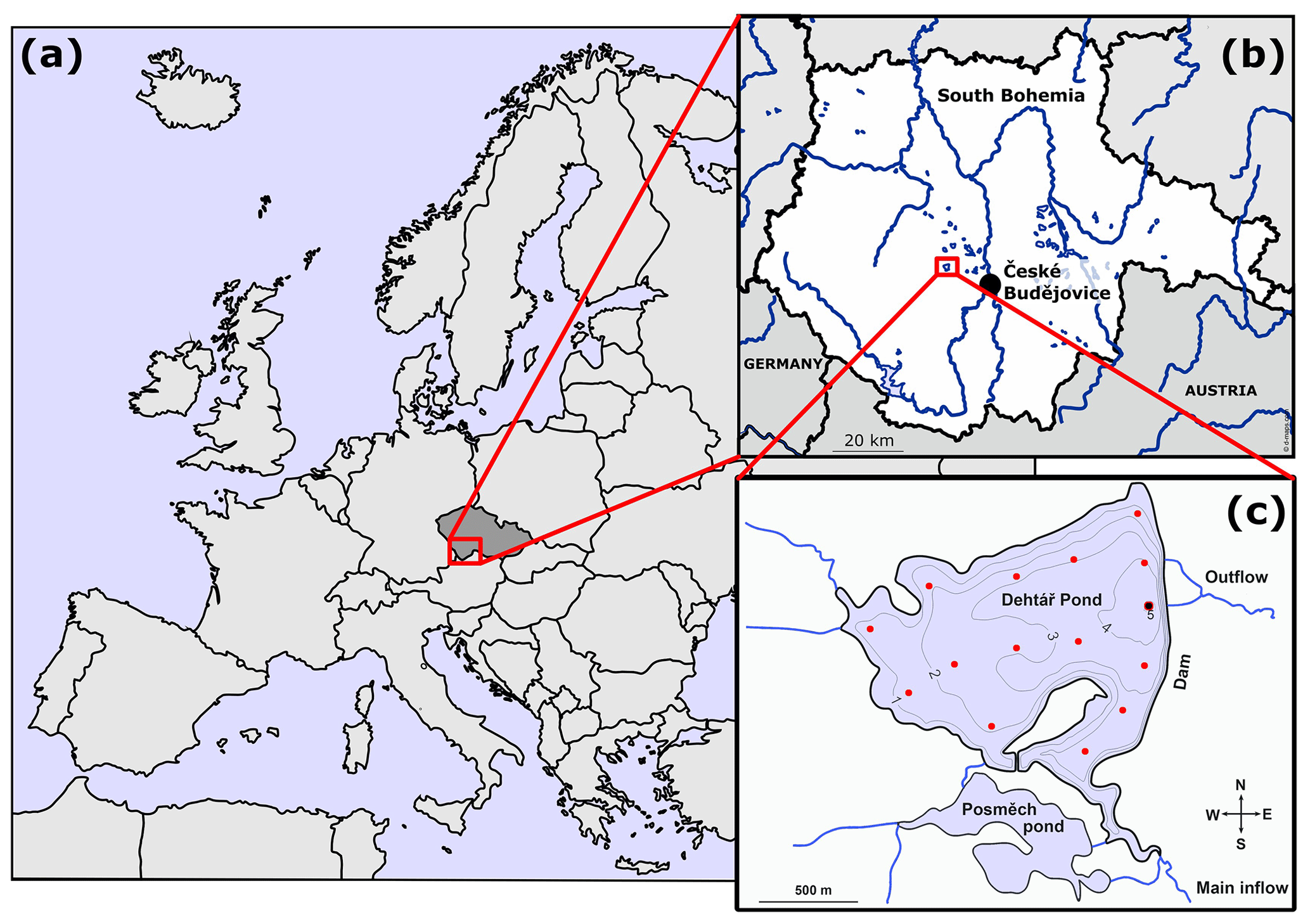
Figure 1Location (a, b; © D-maps.com, 2013a, b; modified) and bathymetric map (c; credited to Jiří Jarošík) of the sampled Dehtář fishpond: blue lines indicate hydrological connections; red dots represent the sampling points. Highlighted sampling point at the dam depicts the deepest site where vertical profiles were measured. Numbers indicate isobath depth.

2.2 Sampling design and measurement

To measure spatial heterogeneity and temporal changes in limnological parameters and methane fluxes, we conducted three surveys each of 36 h in summer 2019 (2–3 July, 13–14 August, 19–20 September). In the morning (between 05:00–06:00 LT), we first measured surface values and vertical profiles of temperature, oxygen, and chlorophyll a concentration at the deepest point (see later for details). We subsequently installed 15 floating polyethylene chambers (as shown in Fig. 1c), serving as fixed sampling sites and at the same time for accumulation of CH₄ fluxes (see further), starting in the western part of the fishpond. During installation (and during each sampling), temperature, pH, and oxygen concentrations were measured at 0.3 m depth using the WTW 330i pH meter, and oximeter (WTW, Weilheim, Germany). Vertical chlorophyll a profiles were measured at each sampling site using a submersible fluorescence probe (FluoroProbe, bbe Moldaenke, Kiel, Germany). From each site, the average chlorophyll a concentration in the surface layer (0–1 m depth) was used to assess the phytoplankton spatial heterogeneity.

To minimise the chance that the differences observed among sites were due to the time of day, we conducted repeated measurements at the deepest point at the end of each sampling. This was relevant mainly to the initial measurement, when the installation of all floating chambers took a total of 3 h and 50 min. All other measurements, i.e. the interval between the first and last sampling point, required approximately 2 h each. If there was a change all values were corrected for the sampling time by linear interpolation:

where P_corr is the corrected value of a parameter, P_t is its value measured at the time t, P₀ and P_end are parameter values measured at the deepest point at the start (time t₀) and at the end (t_end) of the sampling. In the evening and morning of the second day (roughly a 12 h interval), we performed additional measurements of spatial heterogeneity, allowing us to assess diurnal and nocturnal changes. In addition, samples for measuring CH₄ concentration in the surface water were collected at each site and analysed as described later. To assess diurnal variations in thermal structure and oxygen concentration in the water column, we made vertical profile measurements at the deepest point (Fig. 1c) at 3–6 h intervals using the YSI EXO 2 multiparametric probe (YSI Inc., Yellow Springs, USA).

2.3 Methane measurements

Water samples for determining CH₄ concentrations in the surface water were collected at all 15 sampling sites in triplicate into 20 mL glass bottles. The bottles were capped bubble-free under water with black butyl rubber stoppers (Ochs, Germany) and sealed with aluminium crimps. Immediately after sampling, the water samples were preserved by injecting 100 µL of concentrated sulfuric acid to stop the microbial activity (Bussmann et al., 2015). The samples were processed within one week in the laboratory using a headspace technique according to McAuliffe (1971). The methane concentration in the headspace was measured using an HP 5890 Series II gas chromatograph (Agilent Technologies, USA) and calculated with the solubility coefficient given by Yamamoto et al. (1976).

Methane diffusive fluxes (F) were then calculated for each sampling site indirectly using the two-layer model with the equation:

where C_sur is the CH₄ concentration in surface water in µmol L⁻¹, C_eq is the CH₄ concentration in surface water in equilibrium with the atmosphere in µmol L⁻¹, and k is the CH₄ exchange constant (cm h⁻¹). The atmospheric partial pressure of CH₄ was set to 1.8 ppm. To compute k values, we first derived k₆₀₀ estimates using a wind speed-based relationship according to Crusius and Wanninkhof (2003):

where U₁₀ represents the wind speed at a height of 10 m (in m s⁻¹; obtained from the nearby gauging station) approximated by U₁₀=1.22 U, where U is the wind speed at 1.5 m height. We then converted k₆₀₀ to k using the Eq. (4) according to Crusius and Wanninkhof (2003):

where k₆₀₀ is the gas transfer velocity for a Schmidt number (Sc) of 600; n is a wind speed-dependent conversion factor, for which we used $-\mathrm{2}/\mathrm{3}$ for U₁₀<3.7 m s⁻¹ (Jähne et al., 1987). The Schmidt number for CH₄ was calculated according to Wanninkhof (2014):

where t (^∘C) is the water temperature at the time of CH₄ extraction. The parameter C_eq in Eq. (1) was determined from the equation:

where β is the solubility coefficient of CH₄ as a function of temperature according to Wiesenburg and Guinasso (1979), and pCH₄ is the partial pressure of CH₄ in the atmosphere.

To estimate total CH₄ fluxes from the water column to the atmosphere (i.e. diffusive and ebullitive fluxes), we measured CH₄ accumulation in open-bottomed floating polyethylene chambers (volume 3.1 L, area 0.024 m²). Each gas chamber was anchored at 15 individual fixed sampling sites but allowed to float freely on the water surface. Gas was allowed to accumulate for approximately 12 h (each incubation had a starting and end point) during a particular sampling period, i.e. during the day and night periods. Afterwards, 30 mL of gas was carefully taken from each chamber, after mixing the headspace in the chamber, and stored in evacuated Exetainers^® (Labco Limited, UK). Chambers were ventilated after each sampling period to reset the incubation conditions. Methane fluxes were calculated as the difference between initial background and final concentrations in the chamber headspace and expressed as the 1 m² area of the surface level per day according to Bastviken et al. (2004).

2.4 Background limnological parameters

During each campaign water samples for analysis of nutrient concentration and phytoplankton composition were collected from the surface at the deepest point using a Friedinger sampler. Water transparency was measured using a Secchi disc. Total phosphorus (TP) and soluble reactive phosphorus (SRP) were analysed spectrophotometrically according to Kopáček and Hejzlar (1993) and Murphy and Riley (1962), respectively. Concentrations of NH${}_{\mathrm{4}}^{+}$ and NO${}_{\mathrm{3}}^{-}$ were determined according to the procedure of Kopáček and Procházková (1993) and Procházková (1959), respectively. Phytoplankton samples were preserved with Lugol's solution and examined for species composition with an inverted microscope (Olympus IMT-2). Weather data were obtained from the gauging station at the fishpond dam.

2.5 Statistical analyses

Two-tailed paired Student's t tests and two-way ANOVA with post hoc Tukey's multiple comparison test (Prism 9.3, GraphPad Software Inc., La Jolla, CA, USA) were used to test for differences between diffusive and total CH₄ fluxes between day and night and among three sampling campaigns. The percentage of data variability explained by different factors (daytime, month and site) was calculated with the two-way repeated measures (RM) ANOVA. Contour graphs illustrating changes in spatial heterogeneity of measured parameters were constructed in Surfer 10 (Golden Software Inc., CO, USA) using the kriging contouring method. Spatial heterogeneity was quantified for each sampling by calculating the spatial variance (i.e. coefficient of variation of values measured at 15 sampling sites; see, e.g. Fig. 2):

Higher spatial variance indicates increasing ecosystem patchiness. Linear mixed-effects models were used to analyse the effects of O₂, pH, temperature, and water depth on the CH₄ diffusive fluxes with the random effect of time of day nested within the effect of the sampling date. The most parsimonious model was obtained by a manual backward selection, where we sequentially removed all insignificant predictors (p>0.05) using likelihood ratio tests implemented in the drop1 function (Zuur et al., 2009). We also compared the slopes of the month-specific regression lines produced by the model using analysis of covariance (Zar, 1984). Linear mixed-effects models were implemented in the lme4 package version 1.1-21 (Bates et al., 2015), and Kenward–Roger F tests were computed using the ANOVA Type II function from the pbkrtest package version 0.4-7 (Halekoh and Hojsgaard, 2014). The prediction of the resulting final model was visualised in the package ggeffects version 0.14.1 (Lüdecke, 2018). Package performance version 0.4.4 (Lüdecke et al., 2020) was used to calculate Nakagawa's R² of the linear model. The statistical analyses were performed using R software (v. 3.5.2, R Core Team, 2018).

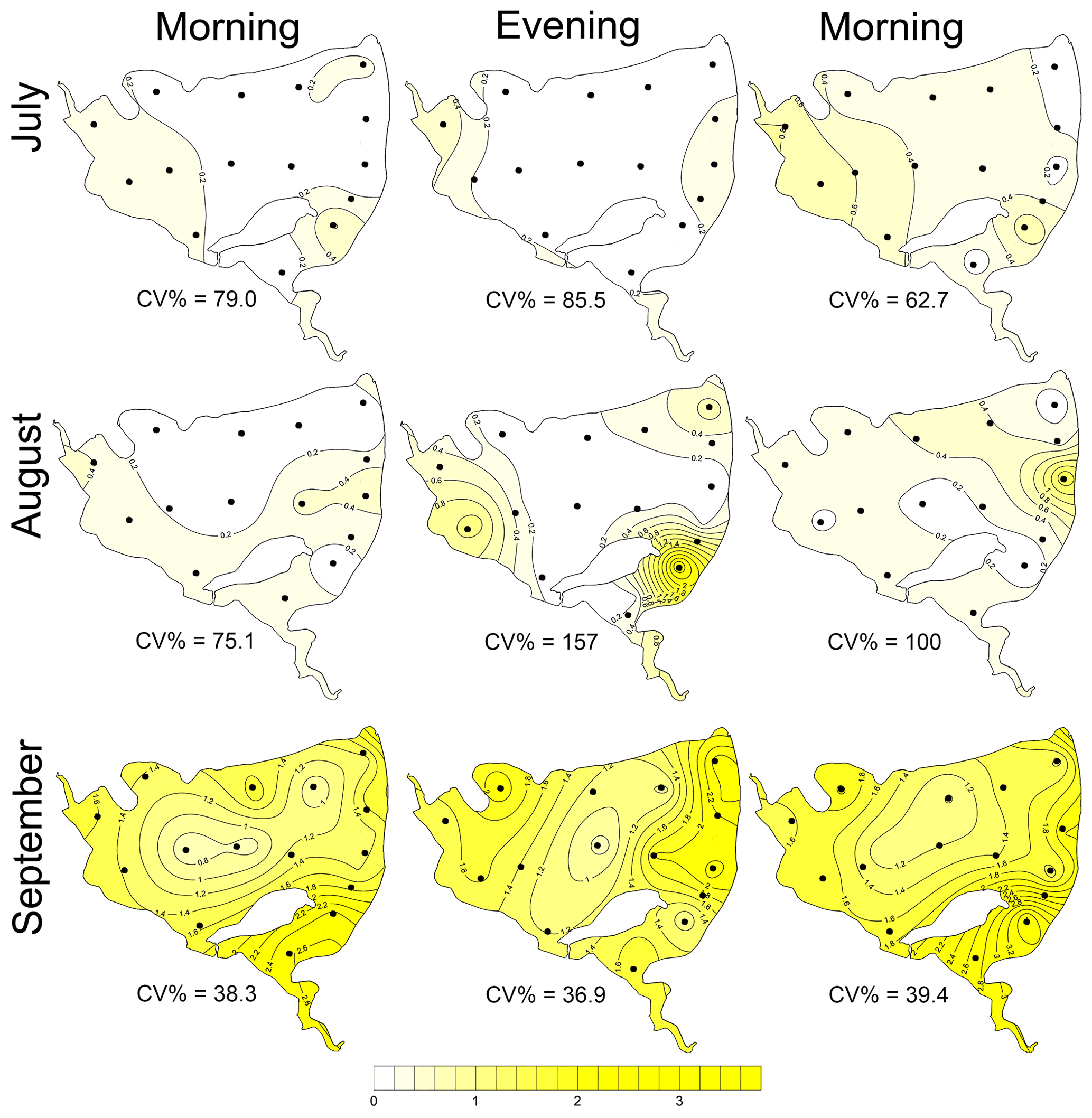
Figure 2Surface methane concentrations (µmol L⁻¹). Contour graphs illustrating both seasonal and daily changes in spatial heterogeneity (indicated by the coefficient of variation, CV %) in the Dehtář fishpond. Black dots represent the sampling sites.

3.1 Weather and background fishpond characteristics

Weather parameters varied among sampling campaigns. In July, clear skies prevailed with the daily air temperature above 30 ^∘C (Table 1). During the August and September measurements it was very cloudy and daily air temperatures decreased to 22 and 18 ^∘C, respectively. The water level was stable during the whole study period with a monthly fluctuation of ∼10 cm. Water transparency was low (15–40 cm), with an increasing trend towards the end of summer (Table 1). Concentrations of total phosphorus and soluble reactive phosphorus were high (Table 1), consistent with a hyper-eutrophic state of the fishpond. In contrast, nitrogen concentrations were relatively low, with ammonium nitrogen being the predominant form of inorganic N in the water (Table 1).

Table 1Basic characteristics of the Dehtář fishpond during the studied period, measured at the surface at the deepest point.

Download Print Version | Download XLSX

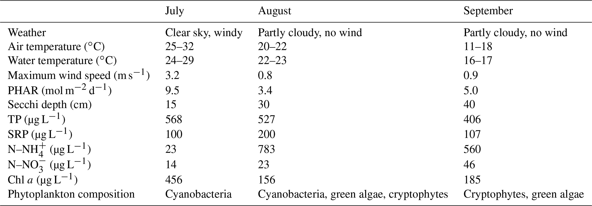
Chlorophyll a concentrations were highest in July due to the dense cyanobacterial bloom accumulated at the surface (Table 1). The phytoplankton consisted of only three cyanobacterial taxa: Dolichospermum flos-aquae, Planktothrix agardhii, and Raphidiopsis mediterranea, and Cuspidothrix issatschenkoi. In August, the phytoplankton was more diverse but also dominated by cyanobacteria: P. agardhii, Aphanizomenon issatschenkoi, and D. flos-aquae. In September, cyanobacteria were absent and instead, cryptophytes (Cryptomonas reflexa), green algae (Pediastrum, Coelastrum and Desmodesmus) and dinoflagellates (Ceratium hirundinella) prevailed.

3.2 Methane concentration and fluxes

The CH₄ concentration in surface water was highly supersaturated over the whole study period. The values obtained varied from 0.003 up to 3.75 µmol L⁻¹ (Fig. 2), which corresponded to saturation levels of 108 %–12 834 %. It is obvious that the obtained data showed remarkable variance: the mean (± SD) values were 0.22±0.18 for July, 0.34±0.45 for August, and 1.61±0.61 µmol L⁻¹ for September (Fig. S11).

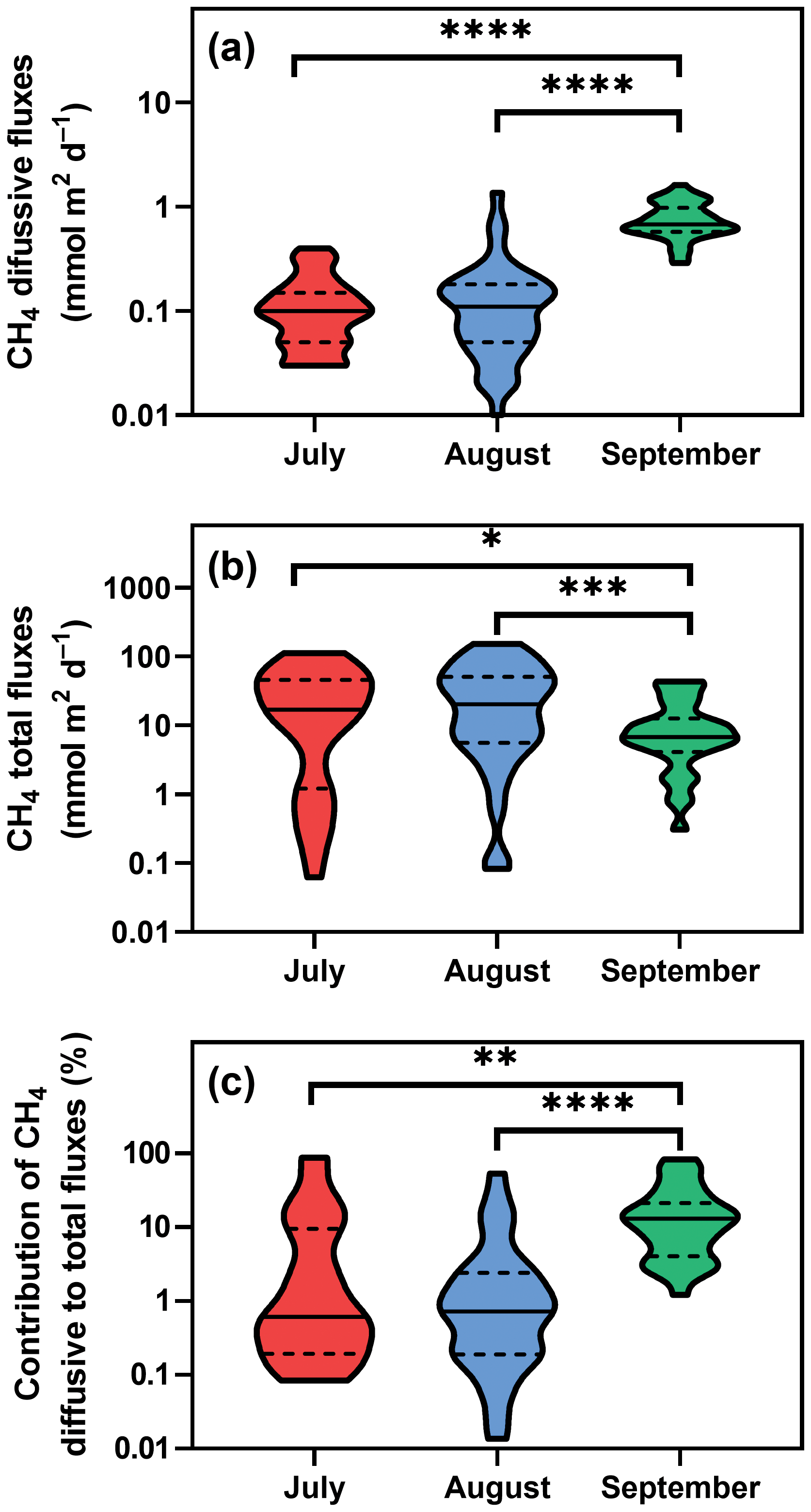
Figure 3Violin plots of CH₄ diffusive (a) and total fluxes (b) during the studied period. Panel (c) depicts differences in the percentage contribution of diffusive to total fluxes. Solid lines are medians, and dashed lines denote quartiles. Asterisks indicate significant differences (^* p<0.05, ${}^{**}$ p<0.01, ${}^{***}$ p<0.001, ${}^{****}$ p<0.0001) between sampling dates determined by two-way ANOVA with Tukey's multiple comparison test. Note that a log scale is used here for clarity.

Download

Diffusive fluxes (i.e. calculated from CH₄ concentration, see Eq. 2) showed the lowest values in July and August (average 0.12 and 0.16 mmol m⁻² d⁻¹, respectively) and pronouncedly peaked in September (average 0.78 mmol m⁻² d⁻¹, Fig. 3a). By contrast, in July and August, the average total CH₄ fluxes (obtained with floating chambers) showed the highest values (average 31.8 mmol m⁻² d⁻¹; ranging from 0.08 to 152 mmol m⁻² d⁻¹) while in September, total CH₄ fluxes were 3 times lower than before (average 11.8 mmol m⁻² d⁻¹, range 0.3–43.5 mmol m⁻² d⁻¹, Fig. 3b). As a result, diffusive fluxes accounted for only a minor fraction of total CH₄ fluxes to the atmosphere (on average, 9.2 % in July, 4.1 % in August and 18.5 % in September, Fig. 3c).

The total CH₄ fluxes showed spatial variability within the fishpond that ranged over four orders of magnitude (Figs. 3, 4 and S11; Table S1 in the Supplement). The observed spatial pattern showed high temporal variability on both daily and monthly scales (Figs. 2 and 4, Table S1). Most of the variability in CH₄ diffusive fluxes was explained by the sampling date (62.4 %), while for the total CH₄ fluxes, spatial heterogeneity accounted for 87.2 % of data variability (Table 2). Using linear mixed-effects models, we identified water depth as the only significant predictor of total CH₄ fluxes (df=1, p<0.0001, marginal Nakagawa's R²=0.348; Fig. 5).

Table 2The percentage of data variability explained by different factors (daytime, month = sampling date, and site) calculated with the two-way repeated measures ANOVA. Statistically significant values (p<0.01) are in bold type.

Download Print Version | Download XLSX

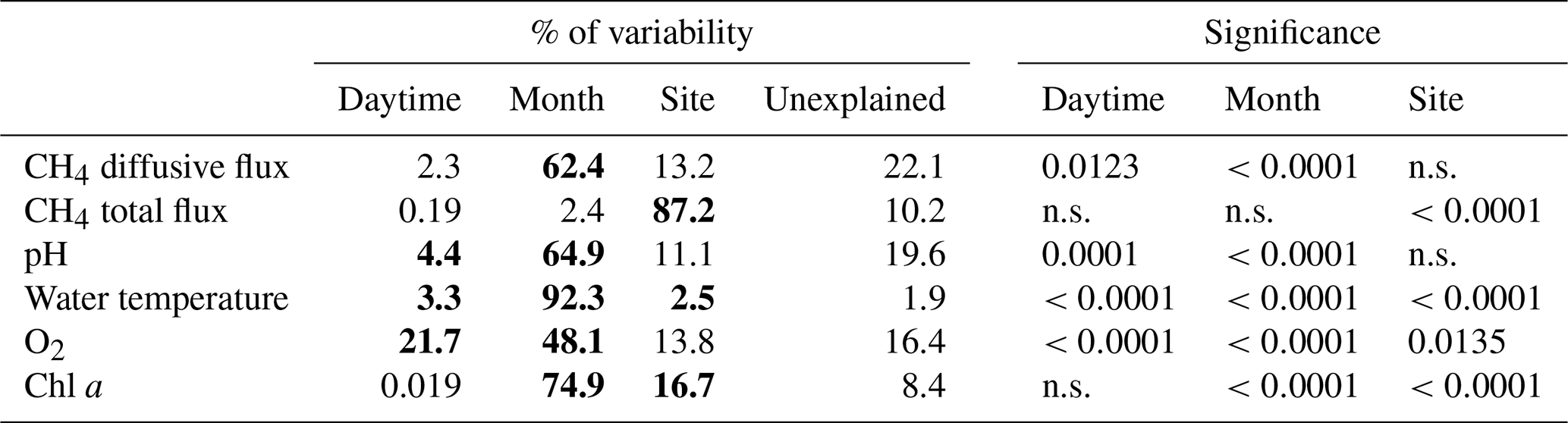
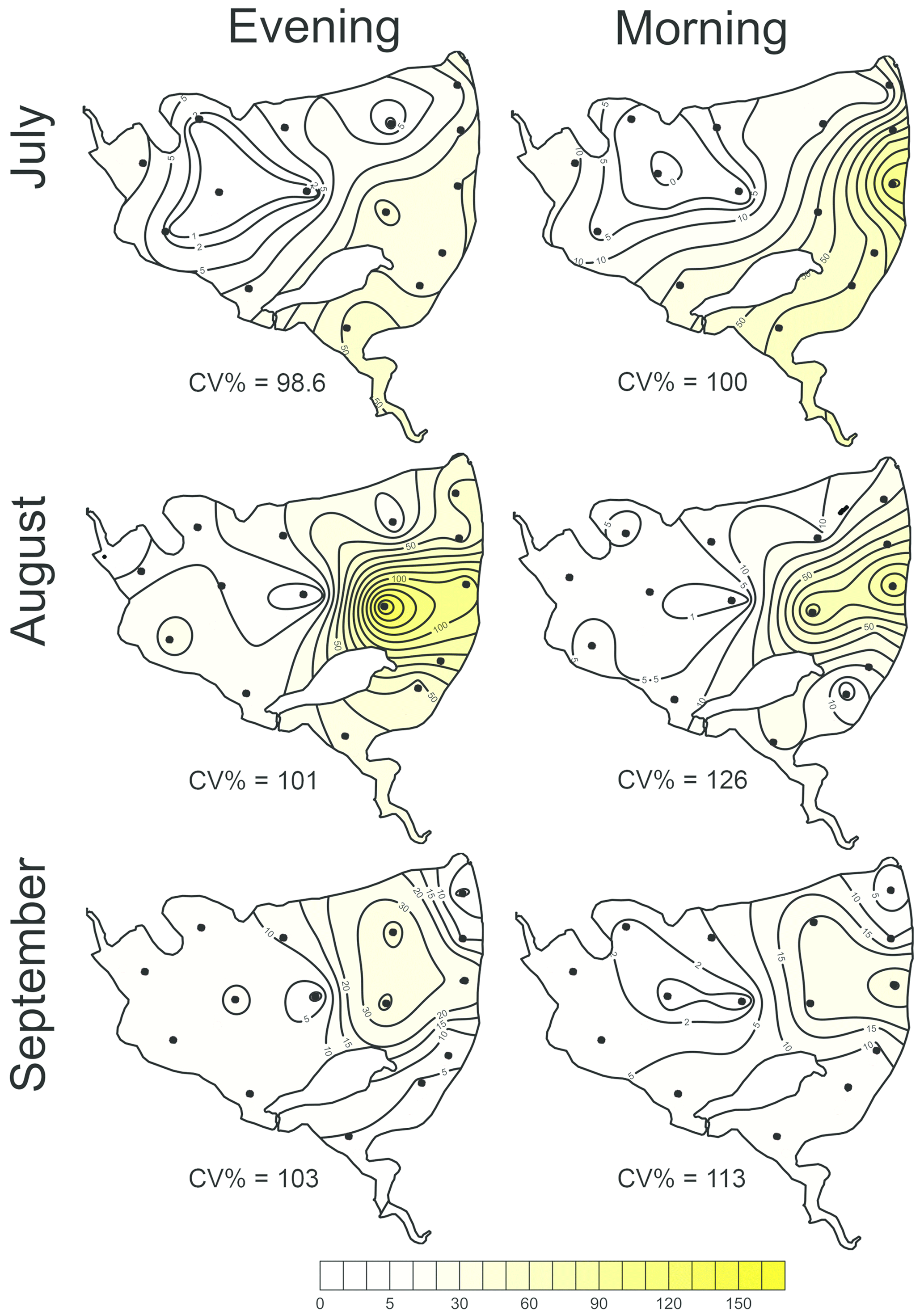
Figure 4Contour graphs of methane total fluxes in the Dehtář fishpond. Isopleths connect sites with the same value of methane fluxes (mmol m⁻² d⁻¹). CV % is a measure of spatial heterogeneity. Black dots representing the sampling sites.

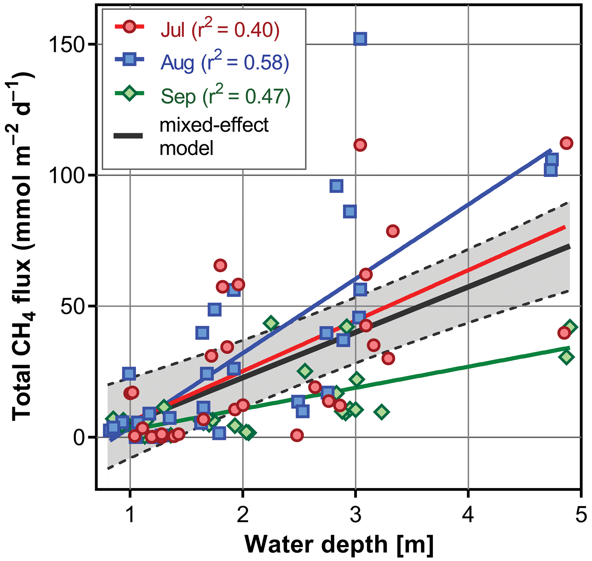
Figure 5The most parsimonious linear mixed-effect model of methane total fluxes showing the water depth as the only significant predictor. Symbols are the measured values, the solid black line is the prediction, and dashed lines are 95% confidence intervals. Colours indicate the month-specific relationship between total methane fluxes and water depth. Differences in slopes were tested using the F test. In September the slope of the regression line was significantly different from those in July and August.

Download

Interestingly, the slopes of the linear regressions differed significantly among individual sampling campaigns (Fig. 5), indicating an additional season-related factor that affects CH₄ fluxes in the fishpond. Calculated CH₄ diffusive fluxes were not correlated with total fluxes. Linear mixed-effects models did not identify any significant predictor of the fluxes, indicating that factors and processes out of the study's scope are involved. We found no significant difference in either diffusive or total CH₄ fluxes between day and night.

3.3 Diurnal changes in vertical profiles of oxygen and temperature

Several contrasting patterns of vertical temperature and oxygen profiles occurred during summer 2019. Diurnal changes were most pronounced in July (Fig. 6). Surface temperatures varied from 25 ^∘C in the morning to nearly 30 ^∘C in the afternoon. Thermal stratification of the water column was weak in the morning but became strongest at 14:30 LT with a thermocline at 0.5 m depth (Fig. 6). Later in the afternoon, the water column began to be mixed by wind. The morning vertical oxygen profile was characterised by a surface value of 4.3 mg L⁻¹, corresponding to 51 % saturation and anoxia below 3 m.

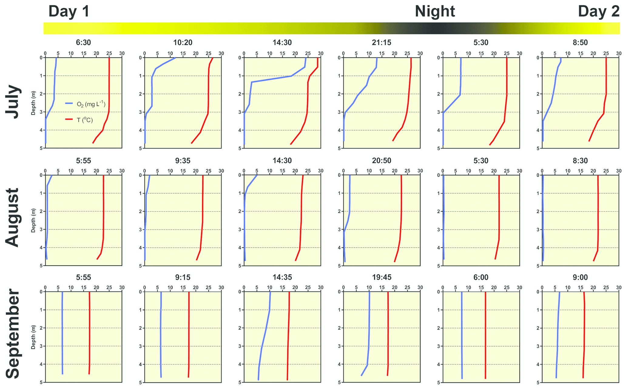
Figure 6Diurnal changes in vertical profiles of temperature and oxygen concentration measured at the deepest point of the fishpond. Numbers above each graph indicate the time of measurement.

Download

Due to the high photosynthetic activity of cyanobacteria, the surface oxygen concentration increased to 24 mg L⁻¹ (320 % saturation, Fig. 6), and a steep oxycline was established at a depth of 0.5–1.5 m with no effect on the anoxic conditions at the deeper layers. Wind action eroded both the oxyclines and thermoclines in the evening, and by the next morning, the vertical profiles were similar to those at the beginning.

In August the water column was almost entirely mixed and low in oxygen in the morning, with only 2.6 mg L⁻¹ (30 % saturation) of oxygen at the surface. Due to cloudy weather, the daily photosynthetic activity of phytoplankton resulted in only a slight increase in oxygen concentration at 0–1.5 m depth (4 mg L⁻¹, 47 % saturation). By the morning of the next day, the entire water column turned very close to anoxic (0.4 mg L⁻¹, 4 % saturation; Fig. 6), which in turn affected the spatial distribution of zooplankton, as evidenced by the formation of dense zooplankton clouds accumulated in the thin layer just at the surface (see Fig. S3). In September, the water column was completely mixed, and we observed only weak daily changes in thermal and oxygen vertical structures (Fig. 6).

3.4 Effect of wind on spatial heterogeneity of temperature, oxygen and chlorophyll a

During the summer all measured parameters showed remarkable within-lake spatial heterogeneity (Figs. S5–S8). In July meteorological conditions enabled demonstration of the effect of wind on fishpond spatial heterogeneity. In the morning, there were no substantial differences in the surface temperature and oxygen concentrations (Fig. 7a and b). The phytoplankton biomass was accumulated mostly in the shallow western part, with the maximum in the centre (Fig. 7c). At 14:00 LT a light breeze started to blow from the northwest, achieving a maximum of 3.2 m s⁻¹ (Fig. S9). This episode lasted until the evening measurement, and the wind ceased by 21:00 LT. The wind was strong enough to substantially change the spatial distribution (Figs. 7d–f and S4). In the evening, the surface water temperature on the windward (south) side of the fishpond was ∼4 ^∘C higher than on the north side (Fig. 7d). The wind also induced order of magnitude differences in oxygen concentration along the north–south axis of the fishpond (3 mg L⁻¹ of O₂ at the north, 24 mg L⁻¹ of O₂ at the south; Fig. 7e) and affected the phytoplankton distribution in the fishpond, resulting in remarkable bloom accumulation in the south (Figs. 7f and S8). During the calm night after the disturbance, the north–south gradient substantially weakened. In August and September the thermal heterogeneity of the pond was relatively low, but the spatial distribution of oxygen and chlorophyll a remained highly variable (Figs. S5–S8, Table S1).

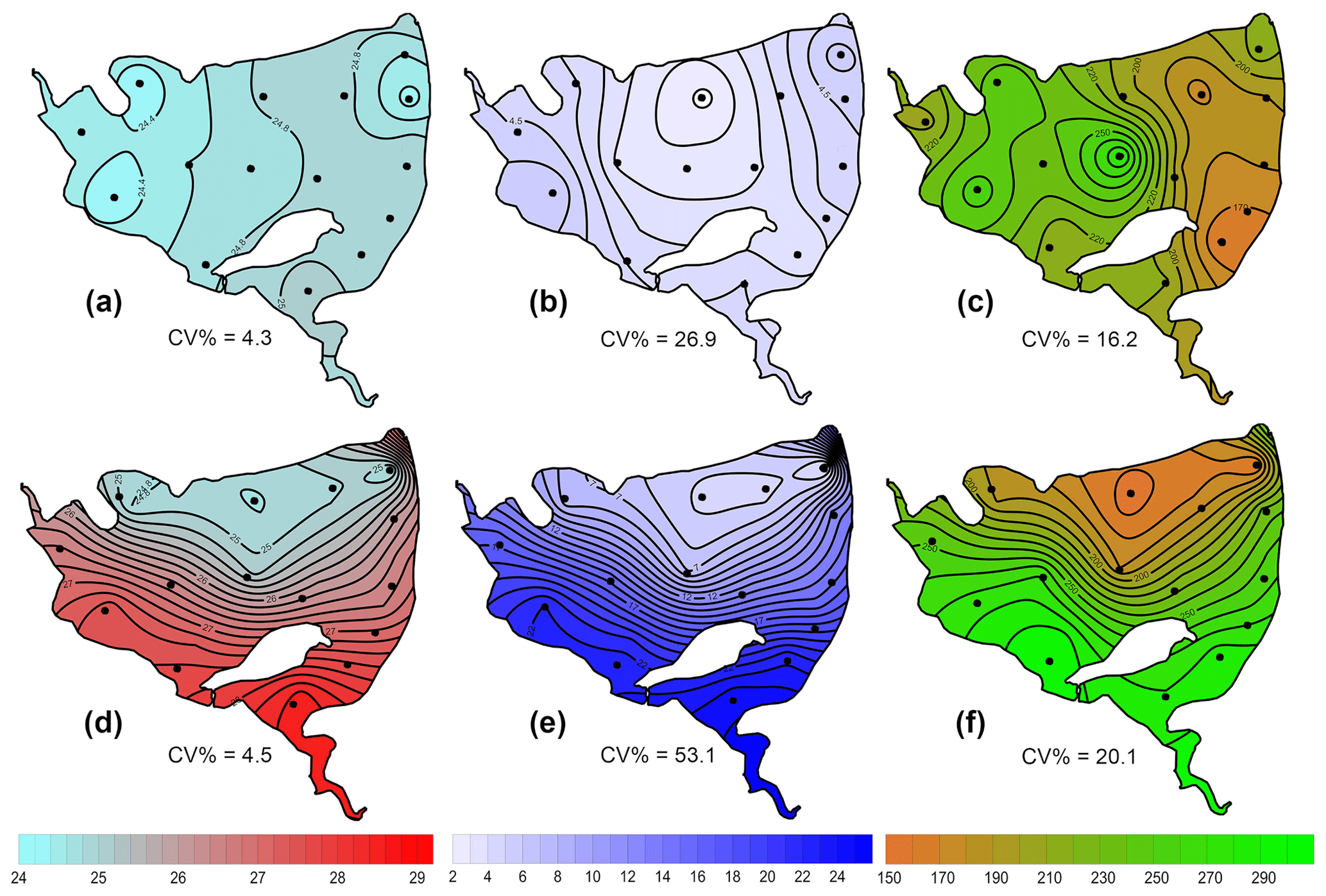
Figure 7Contour graphs of surface temperature (a, d; ^∘C), oxygen concentration (b, e; mg L⁻¹) and chlorophyll a concentration (c, f; µg L⁻¹) measured on 2 July at different times of day: (a)–(c) are the morning measurements; (d)–(f) are evening measurements following a wind disturbance. Coefficient of variation (CV %) is a measure of spatial heterogeneity of measured parameters. Black dots representing the sampling sites.

4.1 Methane fluxes

Assessing the spatial heterogeneity of the CH₄ fluxes within a fishpond is critical for a reliable estimate of its contribution to the global CH₄ budget. In our study, the variability in total CH₄ fluxes spanned several orders of magnitude (ranging from 0.06 up to 1121.3 mmol m⁻² d⁻¹), which is in agreement with similar studies (Casper et al., 2000; DelSontro et al., 2016; Natchimuthu et al., 2016). However, most system-specific CH₄ flux estimates relied on upscaling from a limited number of sites (Bastviken et al., 2004; Rasilo et al., 2015; Wik et al., 2016) because obtaining spatial variability in CH₄ emission is methodologically challenging. In general, spatial heterogeneity may reflect differences in water sources, physical mixing, local transformations and biogeochemical processes and rates among lake habitats (Loken et al., 2019). In deep lakes littoral areas can contribute disproportionately to total lake CH₄ fluxes (Hofmann et al., 2010; Hofmann, 2013; Natchimuthu et al., 2016; Schilder et al., 2013) and are often missed by traditional sampling approaches (Wik et al., 2016). According to Wik et al. (2016), low temporal and spatial resolutions are unlikely to cause overestimates. On the other hand, DelSontro et al. (2018b) suggested that horizontal transport of CH₄ produced in littoral zones and the interaction between physical and biological processes (e.g. air–water gas exchange, water column mixing, the interplay between CH₄ production and microbial oxidation) may result in an underestimation of whole-lake CH₄ fluxes based on centre samples. Similarly, Natchimuthu et al. (2016) found that up to 78 % underestimation would occur if samples obtained only from the lake centre are used to extrapolate the total CH₄ flux. However, extrapolating our data from the deepest point of the Dehtář fishpond would lead to an overestimation of the CH₄ fluxes by a factor of 2.9 (Fig. S12).

The bias introduced by the deepest point measurement appears to be highly variable among systems with different morphology, geographical location, mixing regimes or trophic states. For instance, analysis of 22 European lakes during late summer has shown that spatially resolved CH₄ diffusive fluxes were highly variable for individual lakes, yielding 55 %–300 % differences in the whole-lake estimates (Schilder et al., 2013). Schmiedeskamp et al. (2021) observed an increase in CH₄ fluxes from the shore towards the centre in response to increasing sediment C-content in two shallow German lakes. In line with these findings, our results provide further evidence that spatially resolved data are needed to validate the uncertainties that come from using single-point samples to represent whole-lake processes in hyper-eutrophic systems. As stated by Loken et al. (2019) rather than assuming spatial homogeneity, scaling-up exercises of global carbon budgets should acknowledge the uncertainty that comes from extrapolating from spatially limited data sets.

In the Dehtář fishpond, the total CH₄ fluxes increased with water depth, and this relationship was month-specific. The highest CH₄ fluxes at the deepest points may seem contradictory to previous studies, in which the highest fluxes were typically observed in littoral areas (e.g. DelSontro et al., 2018b; Hofman et al., 2010; Natchimuthu et al., 2016; Schilder et al., 2013). However, these findings are based on studying mostly large, shallow to medium deep oligotrophic lakes where the morphology, trophic state or oxygen regime sharply contrast with the hyper-eutrophic Dehtář fishpond, where the upper 2 m of the water column were oxygen-saturated while the deepest strata were mostly anoxic, i.e. the extent and duration of bottom anoxia could be the most influential factor contributing to the highest methane fluxes at the deepest point of the pond. In hyper-eutrophic systems high nutrient loading increases autochthonous primary production (Potužák et al., 2007; Rutegwa et al., 2019) and promotes oxygen consumption and anaerobic decomposition in the sediments (Baxa et al., 2021), leading to enhanced CH₄ production (Bastviken et al., 2004; Grasset et al., 2018). In aquaculture ponds in southeast China, CH₄ fluxes exhibited considerable spatial variations and peaked in the relatively deep feeding zone, where the large loads of sediment organic matter fuelled CH₄ production (Yang et al., 2020). Furthermore, sediment temperature was the strongest predictor of CH₄ fluxes in shallow ponds with an anoxic hypolimnion (DelSontro et al., 2016; Yang et al., 2020). It is, therefore, reasonable to assume that both temperature and oxygen concentration in the sediment likely contributed to changes in observed CH₄ fluxes during the studied period in our study. Although both parameters were not directly measured in the sediment, it can be deduced from their vertical profiles that the probability of sediment anoxia was highest in August and lowest in September, and the sediment temperature was lowest in September (see Fig. 5).

Our results agree with the generally accepted view that processes other than diffusive fluxes, most likely ebullition, represent the major CH₄ pathway to the atmosphere in hyper-eutrophic ponds used for intensive fish production (Kosten et al., 2020). Although freshwater lakes with high primary production are more likely to have high CH₄ ebullition rates (DelSontro et al., 2016), the dominant role of ebullition was also found across lentic systems differing in size, trophic status and geographical location (Aben et al., 2017). Ebullition accounted on average for 56 % of total CH₄ fluxes in northern ponds in Canada (DelSontro et al., 2016), 49 % and 71 % in two different zones of Lake Taihu (Xiao et al., 2017) and 48–83 % in three Swedish lakes (Natchimuthu et al., 2016; Jansen et al., 2019). The highest contribution was found in the small hyper-eutrophic Priest Pot (UK), where ebullition represented 96 % of the total CH₄ flux from the pond (Casper et al., 2000). Apparently, the contribution of ebullition can vary among systems and will remain uncertain until measurement designs cover enough spatiotemporal variability to yield representative values for the whole ecosystem.

In shallow water bodies, a semi-stable flux of microbubbles was suggested to account for a significant portion of the total CH₄ flux (Prairie and del Giorgio, 2013). When the CH₄ concentration in the water column is above a certain threshold of microbubble density, these microbubbles likely aggregate, fuse, and escape to the atmosphere due to buoyancy (Prairie and del Giorgio, 2013). Even a small fluctuation in hydrostatic pressure (e.g. due to changes in atmospheric pressure) or lake water level was shown to trigger enhanced CH₄ ebullition (Bastviken et al., 2004; Casper et al., 2000; Varadharajan and Hemond, 2012). As ebullition rates increase exponentially with temperature, CH₄ fluxes tend to peak in warm summer months (van Bergen et al., 2019). In our study, the 1 % lower air pressure in July and August than in September, along with bottom anoxia and higher water temperature, could account for the enhanced release of CH₄ bubbles from the sediment (31.7 mmol m⁻² d⁻¹, >90 % of total CH₄ fluxes; Fig. S2). In September, when we observed the lowest water temperatures from the studied period and the oxygen profile was relatively uniform, ebullition accounted for 81 % (11 mmol m⁻² d⁻¹) of the total CH₄ fluxes. The spatially pooled data of the total CH₄ fluxes measured in the Dehtář fishpond varied from 11.8 to 34.5 mmol m⁻² d⁻¹, which is comparable with similar systems elsewhere (e.g. Bastviken et al., 2010; van Bergen et al., 2019; Baron et al., 2022). To sum up, both diffusive fluxes and ebullition must be addressed to understand the magnitude of total aquatic CH₄ fluxes and how their relative contributions vary across and within aquatic systems (Kosten et al., 2020). Moreover, with an improved determination of CH₄ hot spots and the causes, the management of ponds could be changed accordingly and so the overall emissions reduced for example by decreasing P-availability and dredging (Nijman et al., 2022).

4.2 Effect of wind event on ecosystem spatial structure

Sudden changes in ecosystem spatial structure in response to meteorological forcing have rarely been documented (Loken et al., 2019) as they are hard to predict. Research into them using traditional methods requires intensive effort or expensive instrumentation (Ortiz and Wilkinson, 2021), and it remains a matter of luck to obtain a relevant dataset. In the July sampling campaign, we observed a strong impact of the wind on environmental heterogeneity in the fishpond, which was apparent at a sub-daily timescale. Due to the methodological constraints, i.e. lack of initial measurement, we can only speculate about the effect of wind on the total CH₄ fluxes. The northwest wind during the day advected warmed surface water with cyanobacterial bloom from the north basin to the south. In the evening, it resulted in bloom accumulation on the upward side and a north–south gradient of more than 4 ^∘C and 20 mg L⁻¹ oxygen. After the winds dropped the observed gradients declined during cooling at night. We assume that the wind blowing across the pond surface drove buoyant cyanobacteria and surface water downwind and caused an upwelling of deeper, colder, and hypoxic water on the upwind side. This wind-related circulation pattern has been described as a “conveyer belt” in classical textbooks (Reynolds, 2006), held responsible for a disruption of the thermal structure of the water column and the non-uniform spatial distribution of pH, oxygen, CO₂ or CH₄ and also plankton assemblages (e.g. Loken et al., 2019; Natchimuthu et al., 2016; Rinke et al., 2009; Ortiz and Wilkinson, 2021).

Similar to our study, mild winds (∼4 m s⁻¹) were strong enough to redistribute heat and induce lake-wide circulation driving upwelling and downwelling in the 24 m deep Lake Pleasant (Czikowsky et al., 2018). As the wind blows harder and lasts longer, the effects on ecosystem functioning may target higher trophic levels and become more complex (Rinke et al., 2009). In Lake Constance, a 3 d storm event with wind velocities of ∼10 m s⁻¹ resulted in a lake-wide displacement of water masses and the formation of the 6–15 ^∘C horizontal surface water gradient, which in turn changed the spatial distribution of phytoplankton, zooplankton and juvenile fish (Rinke et al., 2009). After several stormy days (wind velocities of 12–15 m s⁻¹), Čech et al. (2011) observed negative effects of wind-driven changes in water temperature and wave action on perch (Perca fluviatilis) spawning in Lake Milada. Although wind events affect shallow and deep lakes differently, there is growing evidence that they can have far-reaching consequences on the functioning of aquatic ecosystems by disrupting energy flows, nutrient fluxes, productivity and reproduction, and consequently altering community composition and trophic interactions in the short and long terms (Stockwell et al., 2020). As the frequency, intensity, spatial extent and duration of these extreme meteorological events are projected to increase due to ongoing climate change (Comou and Rahmstorf, 2012), there is an urgent need for a better understanding of the mechanisms underlying their impacts on the maintenance of the ecosystem services.

4.3 Summer changes in the oxygen regime

Our data demonstrate that shallow, hyper-eutrophic ponds have disrupted oxygen regimes (Baxa et al., 2021) with anoxic hypolimnion and may experience severe whole-water column hypoxia critical for aquatic biota (Miranda et al., 2001). The hypoxic periods may result, for example, from sudden weather change (Jeppesen et al., 1990) and last several days, during which physical processes and phytoplankton photosynthesis cannot compensate for intense community respiration (Baxa et al., 2021). This became obvious in August when severe oxygen depletion was measured at the surface across the whole pond, mostly far below a critical level of 4.5 mg L⁻¹, when adverse effects came into play (Banerjee et al., 2019). However, oxygen surface concentrations in shallow parts of the pond were substantially higher regardless of the time of day, which contrasts with findings of Miranda et al. (2001), who emphasised shallow waters as the most sensitive parts of lakes, where hypoxic events can occur due to the respiration of sediment biota. The observed spatial gradients of oxygen may create temporal refugia which allow fish to survive harsh conditions that occur in the deepest part of the pond. To minimise economic losses and negative impacts on the ecosystem, future research should identify the interplay between meteorological forcing, trophic status and anthropogenic pressures (e.g. management practices) that affect oxygen fluctuations at various timescales.

4.4 Study limitations

Like in other research, there are some limitations in the current study. As our measurement had only a limited temporal resolution (three samplings during the summer season), it is not appropriate to extrapolate CH₄ emissions for annual values. Noticeably, future research must increase the frequency of the sampling and also include innovative techniques to measure CH₄ fluxes at multiple fishponds, with different management regimes. In our study, the 12 h deployment time of the floating chambers could have led to extensive gas accumulation, which in turn might have resulted in an underestimation of the total CH₄ fluxes due to the dissolution of the CH₄ from the chamber into the water once the equilibrium concentration in the chamber is overcome (Bastviken et al., 2010). However, CH₄ concentrations in water corresponded to a supersaturation of several orders of magnitude, so the introduced bias appears to be of minor importance. In any case, our daily spatially pooled total CH₄ fluxes (11.8–34.5 mmol m⁻² d⁻¹) represent a rather conservative estimate for the global methane budget. In our study, we also did not address the important processes that could shed light on the lake CH₄ budget, such as CH₄ oxidation rates (Bastviken et al., 2008) or biological interaction (e.g. protistan grazing on CH₄ oxidising bacteria) in aquatic food webs (Sanseverino et al., 2012) that can affect the overall CH₄ fluxes. We also lack information about spatial differences in sediment microbiota and organic carbon content and compositions, which were found to affect CH₄ production rates (Berberich et al., 2020; Emerson et al., 2021). Despite the limitation mentioned, our results show that complementary spatial surveys help contextualise the fixed station dynamics and provide additional, management-relevant information about the fishpond.

For improved monitoring strategies, however, a continuous measurement approach, such as eddy covariance would be generally more efficient than traditional sampling at regular intervals. Eddy covariance accounts for temporal variability and provides high temporal resolution data by continuously measuring wind speed, gas concentration, and vertical turbulent fluxes to estimate methane emissions (Erkkilä et al., 2018). More importantly, it also offers spatially integrated measurements, averaging emissions over a larger area and therefore accounts for pond spatial heterogeneity. However, it is worth noting that the choice of monitoring approach depends on various factors, including the specific objectives, available resources, and the characteristics of the emission sources. To accurately capture both short-term variability and lake spatial heterogeneity of methane ebullition and diffusion fluxes, the most efficient approach was found to be a combination of continuous measurements with traditional methods including floating chambers, anchored funnels and boundary model calculations (Schubert et al., 2012; Podgrajsek et al., 2014; Erkkilä et al., 2018). This integrated approach would provide a comprehensive understanding of methane emissions, enabling better estimation and more effective mitigation efforts.