2.1 Field site description

Three peatland locations affected by permafrost conditions – the Tourist Station, Storflaket, and Stordalen wetlands (Fig. 1) – situated to the south of Torneträsk Lake near Abisko, northern Sweden (68^∘12^′ N, 19^∘03^′ E; 351 m a.s.l.), were the focus of study. The study sites are in the sub-Arctic climatic zone; the mean annual temperature (MAT) was 0.3 ^∘C, and the mean annual precipitation (MAP) was 347.2 mm between 1990–2020 (http://www.smhi.se, last access: 31 January 2023). The study sites comprise areas of raised palsas (i.e. relatively dry peat plateaus) and waterlogged areas with fen or birch forest vegetation. All three sites show signs of active permafrost thaw indicated by a lowering of the ground surface (i.e. ground subsidence), high soil moisture levels and areas of palsa collapse (i.e. complete permafrost degradation and transition from palsas to wetland) (Åkerman and Johansson, 2008). The raised-palsa parts of the sites tend to get snow free in April–May, but snow can remain in hollows into June.

Previous mapping of the vegetation at these sites using unoccupied aerial vehicles (UAVs) and subsidence estimated using ASPIS InSAR (de la Barreda-Bautista et al., 2022) show the vegetation on the palsas to be composed of bryophytes (e.g. Sphagnum fuscum), lichens and dwarf shrubs (Empetrum nigrum, Andromeda polifolia and Betula nana; (Sjögersten et al., 2016)). The most common herbaceous species was Rubus chamaemorus. Recently collapsed areas adjacent to and within the plateau areas tended to be vegetated by Sphagnum sp. and Eriophorum vaginatum and E. angustifolium. Extensively collapsed and subsequently flooded areas tended to be vegetated by graminoids, mainly Carex and Eriophorum species; herbaceous plants, mainly Menyanthes trifoliata and Comarum palustre; and deciduous shrubs, such as Salix laponica, Salix spp. and Betula nana. Forested-wetland areas tended to be located adjacent to streams and at the perimeters of the wetland areas. The mean peat depth was ca. 60, 94, 50 and 40 cm on palsas, Sphagnum sp., sedge and forested-wetland areas, respectively; the mean soil C storage in the top 100 cm was 52, 34, 33 and 40 kg SOC m⁻² for palsas (soil organic carbon), Sphagnum sp., sedge and forested wetland, respectively (Siewert, 2018). The depth of the active layer (the seasonally thawed upper part of the soil) varies between drier areas, which have a shallower (ca. 30–60 cm) active layer, and wetter areas, where the active layer is deeper or where there is no permafrost at all in the upper 1.5 m. In the Torneträsk area, the active-layer depths have increased, between 0.2 and 2.0 cm yr⁻¹ over 1978–2006, with a higher rate in more recent years (Åkerman and Johansson, 2008).

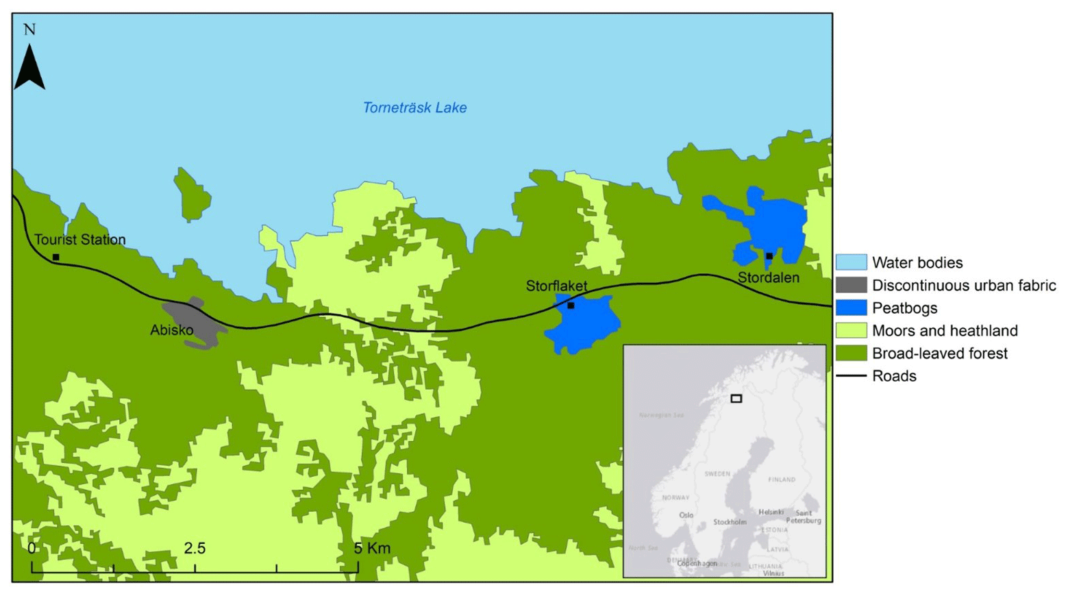
Figure 1Map showing the location of the three permafrost peatland study sites: Tourist Station, Storflaket and Stordalen. The inset is the location of Abisko in northern Sweden. The land cover classes were based on the CORINE (Coordination of information on the environment) land cover classification.

2.2 Experimental design

The fieldwork to measure CH₄ emissions at the three study sites was carried out across the dates of 8–15 June, 18–29 July and 8–12 September 2021. At each site, we targeted six common vegetation types. The vegetation types dry lichen, dwarf shrub, moist moss, Sphagnum wetland, sedge wetland and willow wetland along with the dry lichen, dwarf shrub and moist moss occurred on the drier parts on the palsa. The vegetation types Sphagnum wetland, sedge wetland and willow wetland occurred in waterlogged fen or thermokarst areas. We also measured CH₄ emissions from subsiding areas with the vegetation types dry lichen, dwarf shrub and moist moss subsiding. Areas were identified visually based on changes in topography, subsidence and waterlogging. Measurements in each vegetation type were carried out in blocks of ca. 10 m diameter with three to five sampling points in each block. Sampling blocks were distributed across the sites, and for the majority of vegetation type data from at least two spatially separate (i.e. >100 m apart) blocks were collected. As the vegetation type dry lichen subsiding was not common, this vegetation was sampled less than the other classes. To facilitate the collection of spatially distributed data from the common vegetation types, we selected sites with relatively easy access (e.g. sampling of waterlogged areas was completed in parts of the sites accessible by boardwalks). This approach allowed us to collect CH₄ flux data from a large number of sampling points with the aim of generating scalable data from each vegetation type. A total of 502 measurements were collected across the three sites and the three dates, with all vegetation types measured in several locations at each site. Specifically, on the raised palsas and subsiding-palsa areas, the total number of measurements were 47 and 9 for dry lichen (DL) and dry lichen subsiding (DLS), respectively; 42 and 68 for dwarf shrub (DS) and dwarf shrub subsiding (DSS), respectively; and 50 and 56 for moist moss (MM) and moist moss subsiding (MMS), respectively. In the flooded fen vegetation areas, 102, 78 and 50 measurements were made in Sphagnum wetland (SW), sedge wetland (SE) and willow wetland (WW), respectively. A detailed description of the vegetation types are in de la Barreda-Bautista et al. (2022). Additional measurements of soil temperature and moisture using a Theta probe connected to a Theta-Meter (Delta-T Devices, Cambridge, UK) were carried out at each point where methane emissions were measured. The active-layer depths were determined using a graded metal pole in a subset of plots (ca. 10 of each vegetation type in each of the three mires in June, July and September 2021; de la Barreda-Bautista et al., 2022).

2.3 CH₄ emission measurements

Methane flux measurements were conducted using a dynamic closed chamber connected to a Los Gatos ultraportable greenhouse gas (GHG) analyser (San Jose, California, USA). The Los Gatos analyser uses a cavity ring laser spectroscopy system for detecting CH₄ and allows for the detection of CH₄ in the field. It also has the advantage of being stable over time and not requiring regular calibration. Two types of chambers were used, one 15 and one 40 cm tall; the diameter was 40 cm. The chambers were equipped with two push-fit connectors that acted as an inlet and outlet allowing for the gas to flow from the chamber to the analyser and then to flow back into the chamber. After the chamber was placed on the measuring point, it was gently pushed on a 5 cm deep groove in the peat to create an airtight headspace between the ground surface and the chamber walls. To reduce problems with bubbles being released into the chamber, the chamber was first placed on the ground and then lifted and allowed to vent. The chambers were then placed back on the ground, and the sampling tubes were connected. The soil CH₄ concentration (in ppm) increment inside the chamber was measured every 4 to 6 min, with data automatically recorded every 20 s. If the change in CH₄ concentrations was not linear, the measurement was stopped, chambers were lifted from the soil and a new measurement was taken after CH₄ readings had stabilized.

Trace gas concentrations, determined by the Los Gatos instrument, were converted to mass units using the ideal gas law (Eq. 1). Thereafter, using the slope of the linear change in gas concentration over time and Eq. (2), CH₄ fluxes were calculated. Positive fluxes indicated GHG emissions from the soil into the atmosphere, and negative fluxes indicated uptake of atmospheric GHG by the soil.

where n is the number moles of trace gas (mol L⁻¹), P is the atmospheric pressure (Pa), V is the volume of trace gas per litre of air (L L⁻¹), R is the gas law constant (8314.46 L Pa K⁻¹ mol⁻¹) and T is the temperature (K). F is the calculated flux for either CH₄ (mol m⁻² h⁻¹), slope is the slope of the linear regression (mol L⁻¹ h⁻¹), volume_chamber is the chamber headspace volume (L) and area_chamber is the area of the chamber (m²). Fluxes were converted to µg m⁻² h⁻¹ using the molecular weight of CH₄ (i.e. 16.04 g mol⁻¹, respectively). To avoid excluding very low CH₄ fluxes from the seasonal calculations, fluxes with low r² values were used in the calculation of cumulative emissions. By contrast, high CH₄ fluxes with r²<0.7 were discarded as these fluxes were considered to be either affected by CH₄ ebullition or gas leakage. Seasonal fluxes were calculated to the thaw period (i.e. spring–autumn) by scaling the CH₄ flux measurements made in June, July and September to the length of the spring season, summer season and autumn season, respectively, and then summing these. The length of the three seasons follows a rapid transition due to the high latitude. A typical range was estimated using a combination of the seasonal NDVI (normalized difference vegetation index) and air temperature data. The NDVI data from the Torneträsk valley are available from a 6-year UAV time series (Siewert and Olofsson, 2020; Matthias Siewert, unpublished data), indicating the typical trajectory of rising and falling values during spring and autumn of the snow-free season and an NDVI peak plateau (summer) (see Siewert and Olofsson, 2020). Long-term air temperature data from Abisko are monitored by the Swedish meteorological and hydrological service (http://www.smhi.se, last access: 31 January 2023). We defined the spring period as starting from when the ground became snow free, air temperature rose above 5 ^∘C and soil temperatures at 5 cm depth rose to above zero while the NDVI remained low (<0.25); this coincided with the month of June. We defined the summer growing season as the periods from the start of July when the NDVI increased from the NDVI of the non-growing season of <0.25 to >0.5, soil temperatures were consistently over 5 ^∘C and daily mean air temperatures were mostly 10 ^∘C or above. The NDVI peaked in mid-August with values around 0.7. The summer period included July and August. We identified the onset of autumn by a drop in the NDVI at the end of August that occurred in parallel with a drop in the daily mean air temperature which fell below 10 ^∘C at this time. By the end of September, the vegetation had senesced and the mean daily air temperatures started reaching freezing conditions.

2.4 UAV-captured data for digital elevation models (DEMs) and vegetation mapping

Multispectral and true-colour RGB ultra-high-resolution (UHR) data were captured across Storflaket and Stordalen in 2020 and from the Tourist Station site in 2021 from ca. 106 and 100 m height using a fixed-wing UAV – Sensefly eBee fitted with a Parrot Sequoia multispectral sensor. Imagery was collected during the peak vegetation season in the last week of July and first week of August approximately at noon. The Parrot Sequoia obtained spectral measurements across four bands: green (550 nm ± 40 nm), red (660 nm ± 40 nm), red edge (735 nm ± 10 nm) and near infrared (790 nm ± 40 nm). The images, ranging between ∼ 1300–2000 per flight, were processed using Pix4D version 4.6.4 (Berlin, Germany) to produce an orthomosaic for each spectral band. Radiometric calibration was performed using spectral reflectance targets (MosaicMill). This resulted in a ground resolution of ∼ 11–13 cm for the multispectral and 2–3 cm for the RGB data. To ensure the orthomosaic and DEM generated from the UAV data were accurately geolocated, we collected ca. 50 ground control points using a differential GPS (dGPS; Trimble R8s) across all three sites. Further details on the UAV data collection are in de la Barreda-Bautista et al. (2022).

The multispectral UAV data were resampled to 0.5 m spatial resolution and then classified to produce a vegetation type map for the three study sites using the same nine classes (i.e. the dominant vegetation types found on raised-palsa plateaus, dry lichen, dwarf shrub and moist moss, and vegetation and areas covered by those vegetation types impacted by subsidence plus three vegetation types which dominate the flooded areas, Sphagnum moss, sedge and willow wetland) as those for which in situ CH₄ flux data were measured. A support vector machine classification approach (Foody and Mathur, 2004) was used in ArcMap 10.4 (Esri) using the Train Support Vector Machine Classifier in the Spatial Analyst package, with simple random sampling of ground data in June 2021 for the Storflaket (n=258) and Stordalen (n=395) sites and August 2021 for the Tourist Station (n=657) site. The ground points from each site were randomly split into training and validation datasets of 70 % and 30 % proportions. A cutoff of 70 % was used to determine a sufficient level of accuracy for the vegetation mapping. We decided on this threshold because it is high enough to ensure good overall accuracy, whilst it is not so high as to account for the difficulty of mapping classes with very similar spectral signatures, e.g. non-subsiding vegetation classes and their subsiding counterparts. Furthermore, it is also important to note that ground data are never perfect. Indeed, the level of error can be quite large even when arising from authoritative sources. For example, trained aerial-photograph interpreters are known to differ in their labelling of forest classes by up to 30 % in some studies (Powell et al., 2004).

2.5 Sentinel-2 remotely sensed data for vegetation mapping

We used a neural network classification approach (Xie et al., 2008) within R using the “neuralnet” package (https://github.com/bips-hb/neuralnet, last access: 15 May 2023) to predict vegetation cover over the three sites of interest using Sentinel-2 data (wavebands B2, B3, B4, B5, B6, B7, B8a, B11 and B12) and elevation, slope and roughness data derived from the ArcticDEM, an optical stereo imagery model at 2 m spatial resolution (Morin et al., 2016). Cloud-free Sentinel-2 reflectance data from 27 July 2019 were used to produce vegetation maps for the sites of interest. Reflectance data were atmospherically corrected using Sen2Cor in the ESA Sentinel Application Platform (SNAP). Only one image was required to cover the wider study domain. To match the 20 m × 20 m resolution of the Sentinel-2 pixels, average elevation was computed for each pixel. Sentinel-2 wavebands 2, 3 and 4 were resampled from 10 to 20 m resolution using nearest-neighbour interpolation to match the resolution of the other wavebands (Ledger et al., 2023). A Sentinel-2 waveband specification is presented in Table S1 in Supplement S1. The UAV-derived vegetation maps were used to train the Sentinel-2 scenes covering the three study sites Tourist Station, Storflaket and Stordalen. For this the UAV data were upscaled to 20 m × 20 m using majority classification; this yielded a dataset of 2376 pixels. Training and test datasets were created from this. The testing set used was generated as a random stratified sample comprising 50 pixels per vegetation class, unless there was less than that (e.g. the willow wetland class had only 20 test pixels; Ledger et al., 2023).

The neural network approach was used to classify the Sentinel-2 data into vegetation classes from which the total areal extents of each vegetation class across the three sites were calculated. We chose a neural network approach for this purpose because of its ability to build both a hard and soft classification and it is easily implemented in R with rapid processing. Specifically, a multi-layer perceptron network with backpropagation and weight backtracking was used; therefore the “learning rate” and “momentum” parameters were not required (Xie et al., 2008). Two neural networks were generated: one that produced a standard hard classification (i.e. a single class label is produced for each pixel) and one that produced a soft classification (i.e. grades of class membership are produced for each pixel). The approaches of optimal model structure for the majority and the soft classification consisted of 12 principal components, normalized between 0–1; 1 hidden layer with 3 neurons (hard classification) or 10 neurons (soft classification); and an output layer of 15 units corresponding to the land cover types identified within the three study sites. Both models were developed through trial and error and multiple iterations to arrive at the maximum overall accuracy. The soft classification was undertaken as it enables the estimation of the proportion of different vegetation types within each pixel, offering greater understanding of the area covered by each class, in particular to capture and map those smaller patches of vegetation that have a larger contribution to CH₄ flux.

Misclassification errors in the maps may substantially bias estimates of class areal extent generated from the maps. An adjustment for misclassification bias in a map can be made if its accuracy has been rigorously evaluated. Here, good-practice methods for accuracy and area estimation (Olofsson et al., 2014, 2013) were followed to produce misclassification bias-corrected estimates of class area; a bias correction for the soft classification would ideally require more detailed ground reference data than were available. Thus in total, three vegetation type outputs (maps and class areal extents) from the Sentinel-2 data were produced (soft classification, hard classification and misclassification bias-corrected hard classification). The same 70 % accuracy cutoff as described under the UAV mapping section was applied also to the Sentinel-2 datasets. The areal estimates of the vegetation classes were subsequently multiplied by the mean CH₄ fluxes measured for each vegetation class to produce CH₄ budgets for the entire mapped area.

2.6 Surface motion from Sentinel-1 InSAR

We used C-band SAR data from the Sentinel-1 satellites (European Union's Copernicus programme) with a wavelength and frequency of 5.55 cm and 5.41 GHz, respectively, to map multi-annual average velocity, subsequently denoted as the surface motion of the study areas. Details of this approach are in de la Barreda-Bautista et al. (2022). Briefly we gathered images from 2017 to 2020, focusing on the thaw season between April and October for 3 separate years. A total of 125 images were acquired from the descending mode, and surface motion was obtained using the APSIS method (formerly known as the Intermittent Small Baseline Subset, ISBAS), which relaxes the requirement for consistent phase stability for all observations using a coherence threshold of 0.45. Following InSAR processing the ground resolution was 20 m × 20 m. Using a stable reference point located in the centre of the village of Abisko, first the multi-annual average velocity (or average surface displacement) between 2017 and 2020 (with negative values representing subsidence) was calculated and second, for each season, a time series of surface motion was produced, showing the change in relative height of the surface. Surface motion ranges for the 2017 and 2020 thaw periods were calculated by subtracting the minimum surface motion value from the maximum surface motion value within respective time series between June and October. The InSAR data were thereafter compared to the CH₄ flux data as described in the section on statistical analysis below.

2.7 Data analysis

We used residual maximum likelihood (REML) mixed models to test for significant differences in CH₄ fluxes among sites and vegetation and their interactions. For this analysis we used the vegetation type as the fixed effect and sampling location (i.e. block), with the month and site as random effects. The residuals were inspected to ensure the normality assumption of the analysis was met. The standard error in the difference was used to evaluate which vegetation types differed from each other. We tested for the relationships between the UAV-predicted CH₄ budgets per vegetation type and the three different Sentinel-2-based classifications using linear regression analysis. Relationships between ASPIS InSAR linear motion between the 2017 and 2020 thaw periods and seasonal CH₄ fluxes were explored using REML, in which the ground motion categorized into 2.5 mm ranges was used as the fixed effect and the site was used as the random effect. For this analysis comparison, the CH₄ fluxes extrapolated for each target vegetation type to the three sites using the UHR UAV data, which are able to capture the local-scale variation in the vegetation types, were aggregated to the 20 m × 20 m pixel size of the InSAR data.

We also calculated the net emissions of CH₄ across the subsiding parts of the three wetlands (as detected by InSAR). This was done by summing the CH₄ emissions attributed to each subsiding InSAR pixel for all three sites based on the dominant vegetation type (using the UAV vegetation classification) in that pixel. To explore how CH₄ emissions may change as subsidence progresses and results in palsa collapse, waterlogging and vegetation change, we multiplied the currently subsiding wetland areas by the seasonal CH₄ emissions that were measured in the lower- and higher-emitting fen vegetation types, respectively, to generate two exemplar future emissions scenarios. This CH₄ emission scenario “after permafrost loss and palsa collapse” used the assumption that all of the subsiding area will be covered with a particular fen vegetation type. We want to highlight that this is not a realistic scenario as the fen vegetation that will replace the current vegetation on the raised palsas will be a mixture of vegetation communities suited to permanently waterlogged conditions. Hence the calculations of future CH₄ emissions should be viewed as illustrations of the ranges of emissions that could occur from the sites following a full transition to a fen vegetation type based on their current-day emissions.

3.1 Variation in CH₄ fluxes linked to vegetation type and permafrost degradation

The intact vegetation types of raised palsas (DL, DS and MM) generally had low CH₄ fluxes; the vegetation type dry lichen even acted as a weak CH₄ sink in spring (Fig. 2a). The areas identified as showing signs of permafrost degradation/subsidence had higher soil moisture content ($F_{\mathrm{8},\mathrm{489}}=\mathrm{167.91}$, p<0.001; standard error of the difference of SED = 3.6 %; Fig. 3a) and deeper active-layer depths ($F_{\mathrm{7},\mathrm{163}}=\mathrm{27}$, p<0.001 and $F_{\mathrm{8},\mathrm{91}}=\mathrm{8.15}$, p<0.001, for July and September, respectively; Fig. 4) than areas that were less affected by degradation. Degrading areas had elevated CH₄ fluxes compared to the corresponding vegetation types in areas that did not display visual signs of degradation ($F_{\mathrm{8},\mathrm{489}}=\mathrm{8.15}$, p<0.001; SED = 2.85 mg CH₄ m⁻² h⁻¹), with the largest increase in emissions being for subsiding areas of dwarf shrub (Fig. 2). The emissions from the subsiding-palsa areas were highest in summer, corresponding to the period of the highest air and soil temperatures (Figs. 2b, 3). The highest emissions were from the vegetation types of flooded fen, where emissions peaked in autumn (Fig. 2c). Soil temperature peaked in July at the non-flooded sites, while at flooded sites temperatures remained relatively constant after the initial thaw period. The coldest soil temperatures were measured in DS and DSS areas in September ($F_{\mathrm{8},\mathrm{490}}=\mathrm{9.06}$, p<0.001; SED = 0.7 ^∘C).

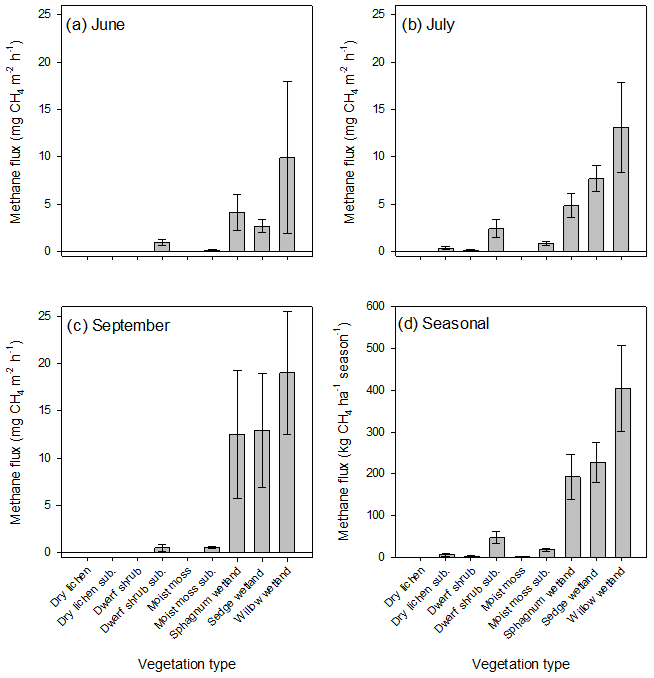
Figure 2CH₄ fluxes measured in different vegetation types in (a) June, (b) July and (c) September and (d) cumulative seasonal CH₄ emissions; sub. denotes measurements made in subsiding areas of vegetation types found on the raised-palsa plateaus. For September, no data are available from the class of dry lichen sub. Means and SE values are shown.

Download

Integrated CH₄ fluxes per vegetation type showed the highest seasonal fluxes of ca. 400 kg CH₄ ha⁻¹ per season from willow wetland areas with emissions from Sphagnum and sedge wetland vegetation types being ca. half those of the willow areas at ca. 200 kg CH₄ ha⁻¹ per season. The seasonal emissions from the areas of dwarf shrub subsiding, moist moss and dry lichen were 50 and 25 kg CH₄ ha⁻¹ per season, respectively, which were higher than in un-degraded areas where emissions from vegetation types of raised palsas were low at less than and/or equal to 2 kg CH₄ ha⁻¹ per season.

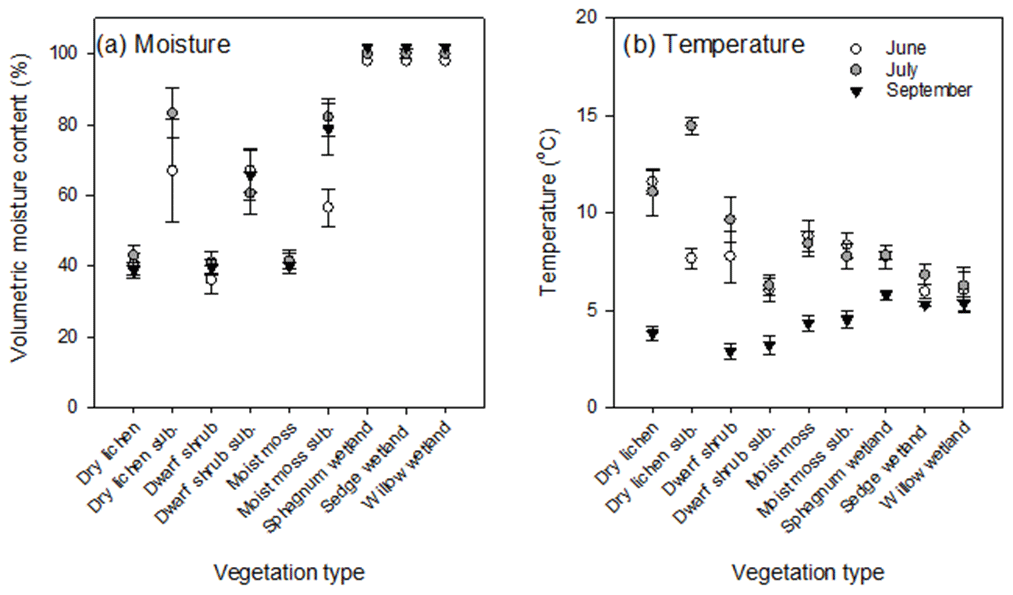
Figure 3Variation in (a) moisture and (b) temperature among vegetation types measured in June, July and September; sub. denotes measurements made in subsiding areas of vegetation types found on the raised-palsa plateaus. For September no data are available from the class of dry lichen sub. Means and SE values are shown.

Download

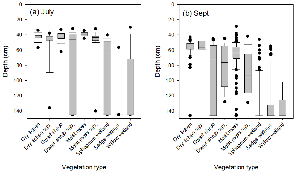
Figure 4Variation in active-layer depth among vegetation types in (a) July and (b) September; sub. denotes measurements made in subsiding areas of vegetation types found on the raised-palsa plateaus. Medians and 25th and 75th percentiles are shown. The whiskers show minimum and maximum values, excluding outliers; the black dots represent outliers.

Download

3.2 Scaling CH₄ fluxes via vegetation mapping and calculation of class areal extent

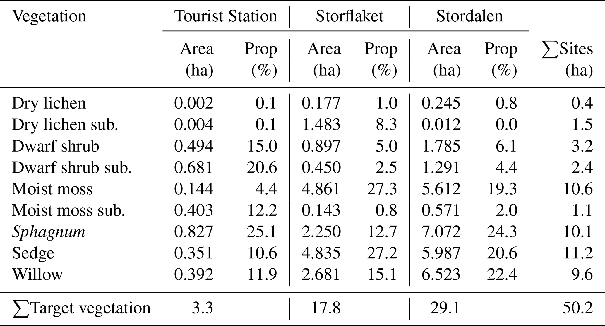
The mapping of the nine vegetation classes found on degrading palsa mires using the UHR UAV data gave an overall classification accuracy of 71 % (confusion matrices were generated in base R; Supplement S2). The area covered by the target wetland vegetation classes (i.e. excluding rock outcrops, birch forest areas, water bodies and anthropogenic surfaces) across the three sites was ca. 50 ha, while the total surveyed area was 83.7 ha (Table 1). Subsequently percentage estimates of areas are made relative to the target vegetation area. Areas where the visual inspection of the surface topography in the field clearly indicated advanced subsidence equated to 10.0 % of the area covered by the vegetation types. The three subsiding vegetation classes covered 1.5, 2.4 and 1.1 ha – or 3.0 %, 4.8 % and 2.2 % of the target vegetation type area – for dry lichen subsiding, dwarf shrub subsiding and moist moss subsiding, respectively (Table 1). The key here was that the classification was of a high enough accuracy for this output to be used as the “ground” data for the Sentinel-2 classifications. We considered 70 % overall accuracy as the threshold for suitable classification accuracy for vegetation classifications. This threshold was decided upon because it is high enough to ensure good overall accuracy, whilst it is not so high as to account for the difficulty of mapping classes with very similar spectral signatures, for example, vegetation classes compared with their subsiding counterparts.

Table 1Area of different wetland vegetation types at each of the three study sites and their proportional (Prop) contribution to the area covered by the target vegetation types. (Please note that areas of anthropogenic surfaces, exposed rock, sparse birch forest on mineral soil, forested wetland and water, as well as pixels impacted by shadows, are not in the CH₄ flux study and hence are not shown in the table.)

Download Print Version | Download XLSX

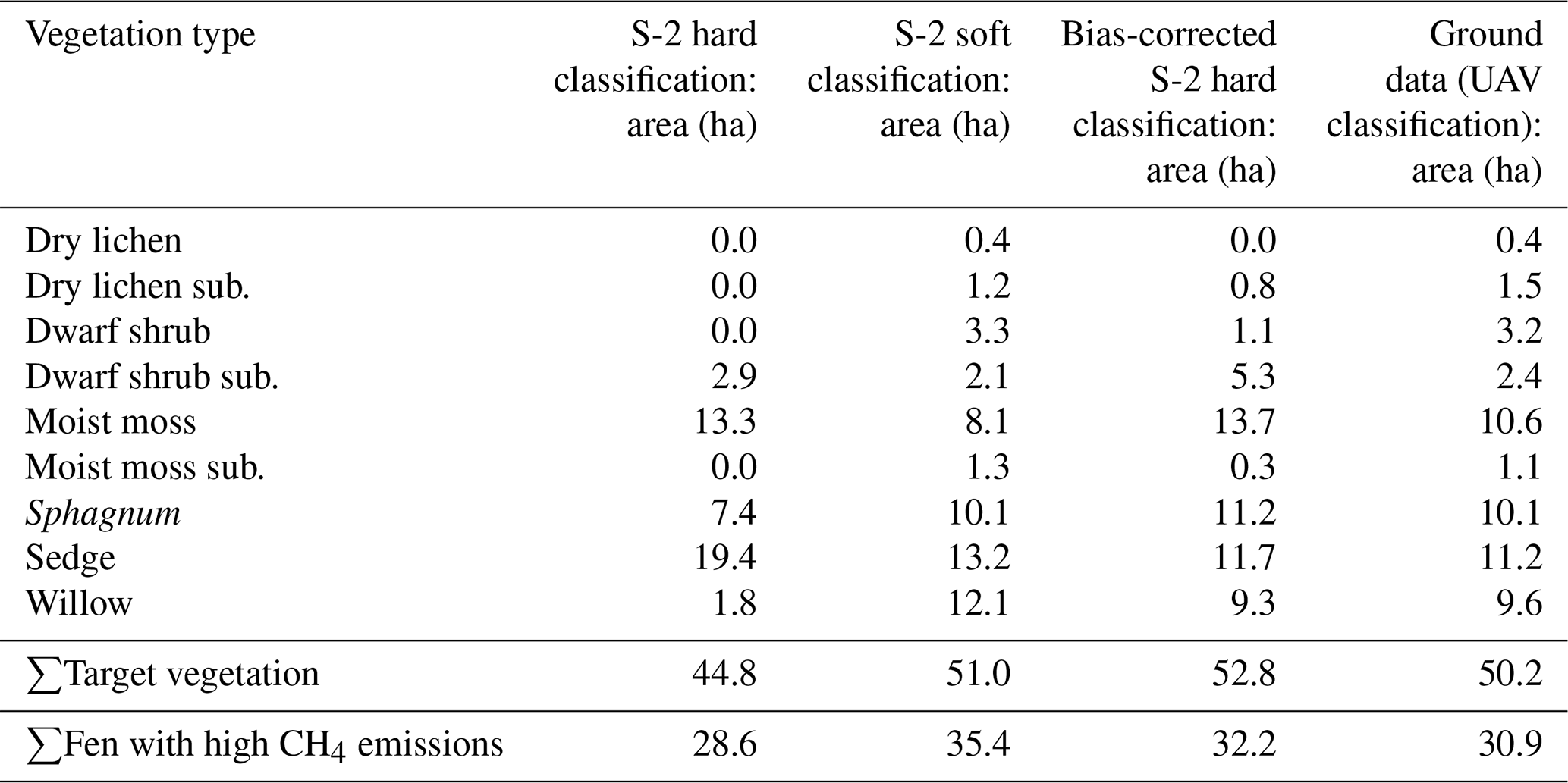
The resultant classification vegetation maps from the Sentinel-2 hard and soft classifications had overall accuracies of 50.2 % and 83.2 %, respectively. The class areal extents from these classification outputs, along with class areal extents obtained when output of the hard classification was corrected for misclassification bias, are presented in Table 2 (which depicts those classes shown in Table 1). The hard classification of Sentinel-2 data did not capture the fine-scale vegetation mosaic on the raised part of the palsa mire (i.e. dry lichen and dwarf shrub prior to subsidence); instead it mapped the vegetation types in those areas as vegetation classes for either moist moss or dwarf shrub subsiding, leading to a lower overall classification accuracy than that obtained using the approach of soft classification. Once corrected for misclassification bias, the areal extents of the hard classification for each vegetation class improved considerably in that the estimates are comparable to that mapped using the UAV data and the soft classification of the Sentinel-2 data. The soft classification of the Sentinel-2 data was able to map all nine target vegetation types and followed the same distribution of more or less abundant vegetation types, predicting total class areal extents similar to that of the UAV-derived maps. In both cases (bias-corrected hard classification and soft classification), those vegetation types on the raised-palsa area missed by the hard classification have a calculated areal extent.

The soft classification of the Sentinel-2 data produced a higher estimate of the areal extent of the fen vegetation types at 35.4 ha than the UAV classification but succeeded in mapping all the vegetation classes present across the study site. The mapping from the hard classification of Sentinel-2 underestimated the vegetation types of fen slightly at 28.64 ha and missed some of the other vegetation classes (i.e. dry lichen, dry lichen subsiding and dwarf shrub). After correcting for classification bias, the areal extents of vegetation classes from the hard classification closely matched those of the UAV-mapped areas, with 32.21 ha of the vegetation types of fen estimated to occupy the study site.

Based on the UAV classification vegetation mapping (class areal extents), 30.9 ha (or 61 %) of the area covered by the target vegetation types was comprised of the three vegetation classes (Sphagnum, sedge and willow wetland – known as vegetation types of fen) associated with the highest CH₄ emissions. Using the mapping of areal extents from the UAV data to model CH₄ fluxes shows marked differences in CH₄ fluxes between raised palsas and the wetland types surrounding these (Fig. 5; Table 3). Areas of the raised palsas, which do not show visual signs of subsidence, generally have very low emissions, while areas with degrading permafrost and subsidence, as well as those areas with no permafrost, emit CH₄. Among the vegetation types that are associated with high CH₄ emissions, the maps highlight the importance of the vegetation type willow wetland as a source of methane from these wetlands. This is because it was both high emissions per area and substantial covered areas in particular at the Stordalen mire site. Although the highest CH₄ emissions are from the areas which have lost their permafrost that are surrounding the remaining palsas, there are indications of increased emissions also within the palsas.

Table 2Comparing class areal estimates for the target vegetation types using Sentinel-2 (S-2) hard and soft classification and bias-corrected hard classification. For comparison the estimates are provided for the UAV-derived classification which served as the ground data.

Download Print Version | Download XLSX

Methane emissions from within the palsa areas are commonly associated with vegetation of moist moss subsiding and dwarf shrub subsiding, as well as development of Sphagnum wetland vegetation in subsiding areas that have become waterlogged either at the edges of the palsas or in their interior following degradation. The vegetation of dwarf shrub subsiding is mainly found along the edges of the palsas that are experiencing lateral erosion, while the vegetation type moist moss subsiding occurs in the interior parts of the palsas in areas with deeper active layers and the development of a hummocky surface.

When CH₄ emissions are integrated across the three wetland areas using the UAV-derived vegetation mapping, net emissions are 8519 kg CH₄ per season (Table 3). The total emissions are composed of 16.6, 142.6 and 8359.5 kg CH₄ per season from the vegetation types of raised palsas (DL, DS, MM), subsiding palsa (DLS, DSS, MMS) and waterlogged (SW, SE, WW), respectively. This shows that currently emissions from intact areas in the early stages of degradation are low compared to the already degraded areas. However, as the areas of raised-palsa vegetation and subsiding-palsa vegetation are large (ca. 20 ha – or 40 % of the area covered by target vegetation types – when combined), there are substantial risks of higher CH₄ emissions from these sites associated with continued degradation of the currently subsiding areas and onset of degradation of the remaining palsa areas.

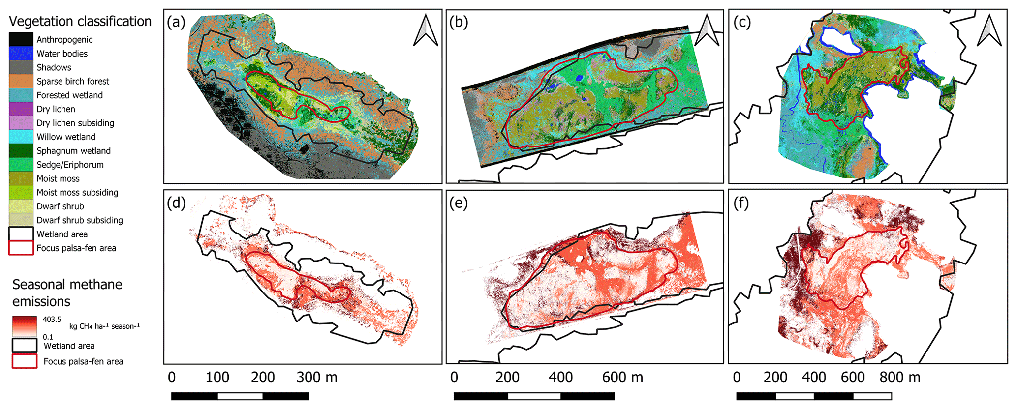
Figure 5(a–c) Detailed vegetation maps separating out wetland vegetation types including vegetation types associated with raised- and subsiding-palsa areas at the Tourist Station, Storflaket and Stordalen mires. The vegetation maps were generated from UAV-captured data. (d–f) Maps of seasonal CH₄ emissions based on the seasonal CH₄ emissions measured in the nine target vegetation types across the three mire sites. The palsa–fen wetland area outlined in purple is the area where ground data for CH₄ fluxes as well as for the vegetation mapping were collected. The full wetland area at each site is indicated by the black boundary line.

Table 3Seasonal methane emissions for 2021 for the total area of each target vegetation class within the area covered by the UAV flights. Methane emissions are estimated for three different models using Sentinel-2 data. The CH₄ flux calculated from the UAV data is derived from the area of each vegetation type multiplied by the seasonal CH₄ flux for each vegetation type. Means and SE values are shown.

Download Print Version | Download XLSX

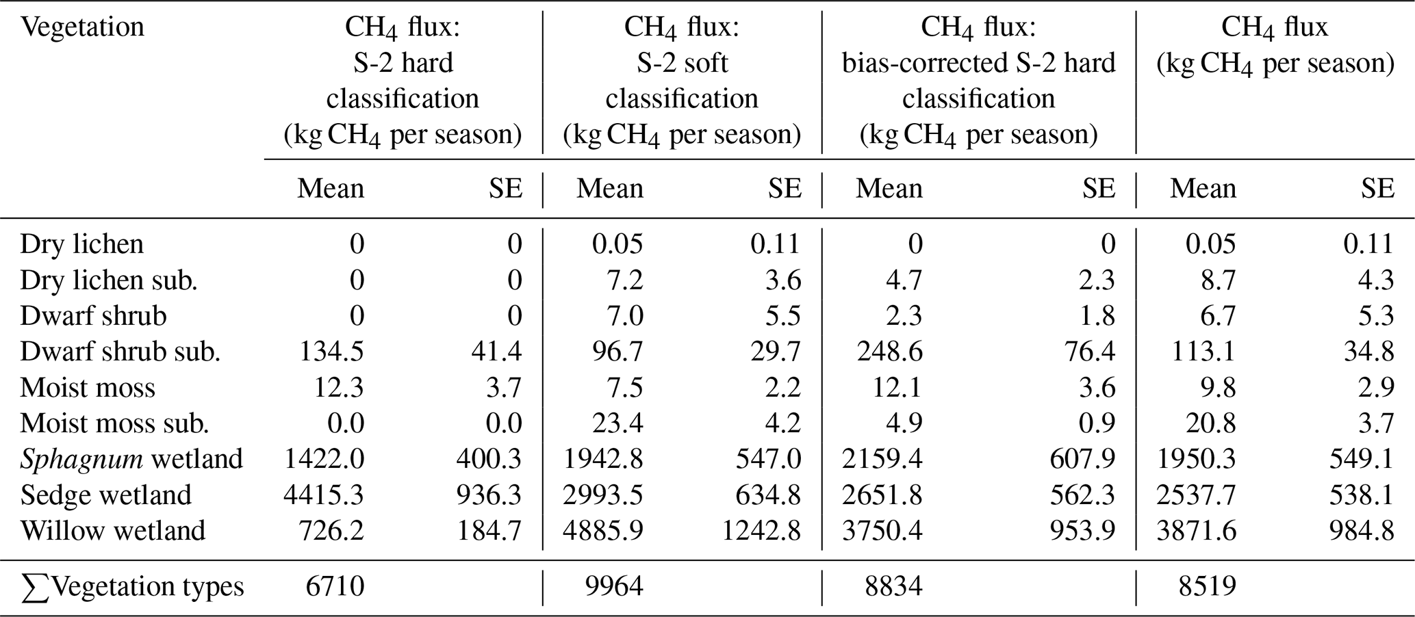
Taking the Sentinel-2 sets of estimates of areal extent of vegetation types to estimate the CH₄ emissions of the vegetation types showed both over- and underestimation of emissions (compared to the UAV-derived CH₄ estimates) – the hard classification underestimated CH₄ emissions across the site by 21 %, while the soft classification overestimated emissions by 17 % (Table 3). The mismatch between the Sentinel-2 hard classification and the UAV estimates was linked to a misclassification of willow wetland as sedge wetland (Table 2, Supplement S2). Correcting the output of the hard classification for misclassification bias improved the match of CH₄ estimates to that derived from the UAV data, and the key was that target vegetation classes were included in the mapping following this post-classification process. For the soft classification, it was the misclassification of sedge and willow wetland area. Correlation analysis between the UAV- and Sentinel-2 classification outputs showed that the bias-corrected hard classification was more closely correlated to the UAV predictions, followed closely by the soft classification with R²=0.99 and R²=0.99 (p<0.001 and p<0.001), respectively. The hard classification was not significantly related to the UAV-predicted CH₄ fluxes (p>0.05; Fig. 6).

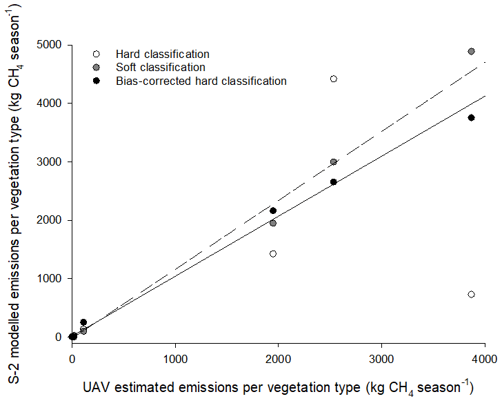
Figure 6Relationship between UAV-estimated methane emissions per vegetation types and the three Sentinel-2 (S-2) models. The dashed and solid lines show the relationships between the soft and bias-corrected hard classification and the UAV-estimated CH₄ emissions, respectively. Note that no regression line was plotted for the hard classification as there was no significant relationship.

Download

3.3 Linking InSAR-determined ground motion to CH₄ emissions

InSAR detected subsidence across 90 % of the study area, indicating that the majority of the surface of these sites was impacted by millimetre level rates of subsidence. However, rates of ground motion varied considerably across the study area and among vegetation types. Importantly, across the three sites, areas with relatively low levels of ground motion were associated with the highest mean CH₄ emissions ($F_{\mathrm{8},\mathrm{1135}}=\mathrm{5.63}$, p<0.001, SED = 961.5; Fig. 7), while both uplifting (5 to 7.5 mm) and the most subsiding (−10 to −12.5 mm) areas tended to have lower fluxes. High cumulative CH₄ emissions (summed over all pixels for a given range of ground motions) were found for areas that were either stable or subsiding at an intermediate rate (Fig. 8), while the most subsiding areas had low cumulative CH₄ emissions.

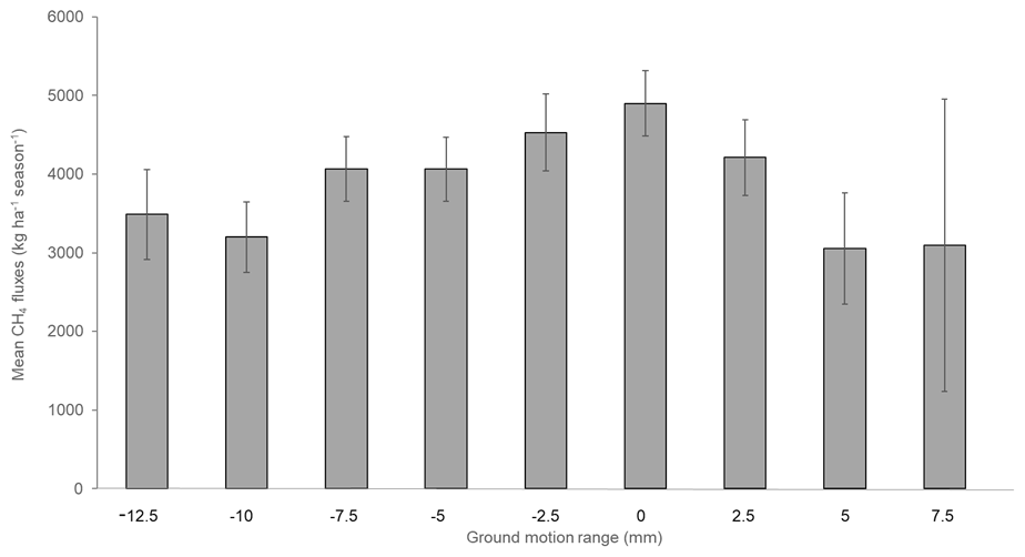
Figure 7Average seasonal CH₄ emissions for different ground motion ranges (categories in 2.5 mm ranges) across the three study sites. Negative values indicate subsidence, and positive values indicate uplift. Means and SE values are shown.

Download

This pattern of areas of high subsidence being linked to areas of low CH₄ emissions was also apparent in the subsidence and CH₄ emission maps (Fig. 9). For example, at the Tourist Station site mire areas of high subsidence (comprising mainly of vegetation of moist moss subsiding; Fig. 5a) corresponded to areas with relatively low CH₄ emissions, while areas that have already transitioned to Sphagnum or willow wetland are associated with bands of high CH₄ emissions along the degrading edge of the palsa plateaus (Fig. 5a and d). Similar patterns were evident at the Storflaket mire, where degrading areas within the palsa plateaus did not display high CH₄ emissions, while areas that have transitioned to Sphagnum or sedge wetland have high CH₄ emissions (Fig. 9b and e). The Stordalen site showed the largest areas of high subsidence that traversed the boundary between the palsa plateau and the fen areas (Fig. 9c and f). In this part of Stordalen the vegetation type Sphagnum wetland was present both in the hollows in the degrading interior of the palsa plateaus and in adjacent areas where the palsas had already collapsed, explaining the high CH₄ emissions (together with the presence of the vegetation type willow wetland) from this area.

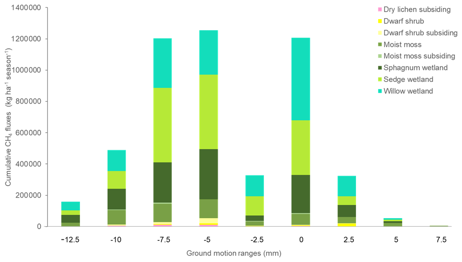
Figure 8Cumulative CH₄ emissions (± SE) for different ground motions across the thaw seasons of 2017 and 2020 for pixels (i.e. a sum of the CH₄ emissions from all pixels of a given ground motion; categories in 2.5 mm ranges) of the target vegetation classes. The vegetation types of dry lichen did not cover large enough areas to be evaluated on the 20 m × 20 m pixel scale of the ground motion data and are therefore not included in this comparison. Negative values indicate subsidence, and positive values indicate uplift.

Download

The net emissions of CH₄ across subsiding parts of the three wetlands (as detected by InSAR) were modest at 116 kg CH₄ per season. However, when these areas have degraded to such a point that they are fully waterlogged and have transitioned to either Sphagnum or sedge vegetation, we estimate emissions from these, currently low-emitting, areas to be around 6480 kg per season or, if we use the highest-emitting vegetation type as a predictor of future emissions, 12 960 kg per season.

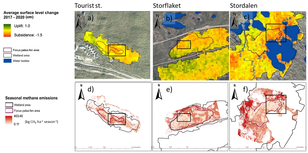
Figure 9Maps of (a–c) ground motion (de la Barreda-Bautista et al., 2022) and (d–f) CH₄ fluxes at the Tourist Station, Storflaket and Stordalen mires. The black boxes show the areas referred to in the text. The backgrounds of (a), (b) and (c) are orthophotos from the area taken in 2018.