In the following, the ESBL flow is introduced forming an idealized model for atmospheric dynamics in reaction to a periodic forcing. Here, three idealized cases representative of diurnal forcing are investigated. The first case is from the Ekman (E) regime that corresponds to a polar boundary layer flow. The second case is from the Stokes (S) regime that corresponds to an ABL flow in the tropics or subtropics. The third case is a near-resonant (NR) one that is representative of critical latitudes at which a boundary layer resonance occurs (e.g., Kerswell, 1995).

Figure 1a shows a sketch of the idealized planar boundary layer configuration considered in this study. A Newtonian fluid resides over a smooth planar surface, which is located at z=0. Both the fluid and the surface are placed in a rotating frame of reference that revolves around the vertical (wall-normal) z coordinate with uniform angular velocity Ω. A flow is driven relative to the rotating frame of reference by prescribed sinusoidal surface oscillations along the streamwise x direction with velocity amplitude U and angular frequency ω. Leading-order Coriolis effects induce flows in the spanwise y direction. The flow is resolved across the height H of the vertically oriented columnar computational domain (“ODT line”) as detailed below. H reaches up into the geostrophic free stream region that is taken at rest relative to the frame of reference. Here, $H/{\mathit{\delta }}_{\mathrm{E}}=\mathrm{360}$, as defined below, has been selected. Note that the set-up is complementary to the pressure-driven flow considered by Salon and Armenio (2011), which is a vertically mirrored version of the laboratory experiment investigated in Vincze et al. (2019), and the planar analog of the curved walls considered by Ghasemi et al. (2018).

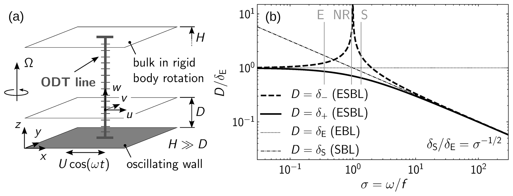
Figure 1(a) Sketch of the ESBL configuration investigated. (b) Various laminar boundary layer length scales D relevant to the ESBL as function of the normalized forcing frequency $\mathit{\sigma }=\mathit{\omega }/f$. Idealized laminar Ekman boundary layer (EBL) and Stokes boundary layer (SBL) thicknesses are given for comparison. The forcing frequencies selected for the turbulent ODT simulations are marked by gray vertical lines. See the text for details.

Download

Next, for the three ESBL cases mentioned above, the emerging multiscale properties are briefly discussed based on the laminar solution of the f-plane equations. This excludes turbulence effects but already hints at key properties of the solution, providing reference length scales for the boundary layer flow. The laminar solution is given by Thorade (1928) for a tidally driven flow, which is similar to Salon and Armenio (2011) who consider a periodically changing pressure gradient and Vincze et al. (2019) who utilize wall oscillations as forcing mechanism. An extended solution for arbitrary wall oscillation frequencies and with an account of leading-order wall-curvature effects is given in Ghasemi et al. (2018). The latter formulation is adopted for the present study but applied to planar surface geometry only. The laminar solution is not repeated here. Instead, only the laminar boundary layer length scales are dicussed below.

The laminar Ekman–Stokes boundary layer is governed by linear dynamics such that a transient but fully periodic solution is obtained. The repeated change of the sign of the wall-shear stress provides an alternating momentum source/sink situation that results in a constant effective boundary layer thickness D. (Experiments have provided evidence that this holds also for turbulent flow conditions for various forcing frequencies, Vincze et al., 2019.) The laminar solution yields four different boundary layer thicknesses, each of which can serve as reference scale D. The length scales are given by the laminar Stokes boundary layer (SBL) thickness ${\mathit{\delta }}_{\mathrm{S}}=\sqrt{\mathrm{2}\mathit{\nu }/\mathit{\omega }}$, the laminar Ekman boundary layer (EBL) thickness ${\mathit{\delta }}_{\mathrm{E}}=\sqrt{\mathrm{2}\mathit{\nu }/f}$, and the two nested layer thicknesses ${\mathit{\delta }}_{\pm }=\sqrt{\mathrm{2}\mathit{\nu }/|f\pm \mathit{\omega }|}$, where f is the Coriolis parameter that is taken as f=2Ω for a notional polar boundary layer, and ν is the kinematic viscosity of the fluid. The relevance of the selected value depends on the forcing as it governs the flow regime.

Figure 1b shows the dependence of the laminar boundary layers on the normalized forcing frequency $\mathit{\sigma }=\mathit{\omega }/f$. The Ekman property dominates for small forcing frequencies (σ≪1) so that D approaches the finite value δ_E from below. The Stokes property dominates for high forcing frequencies (σ≫1) due to which D→δ_S, which is asymptotically smaller than the Ekman layer thickness by the factor ${\mathit{\sigma }}^{-\mathrm{1}/\mathrm{2}}$. This scaling suggests a vanishing boundary layer thickness, $D\simeq {\mathit{\delta }}_{\mathrm{S}}\to \mathrm{0}$, for asymptotically large forcing frequencies. This is more a hypothetical scenario since the wall oscillation aims to model slow processes on the large scales. The limit signalizes that molecular (viscous) surface fluxes are no longer able to respond to the forcing and the forcing only results in high energy dissipation in the vicinity of the surface.

Last, for forcing frequencies comparable to the Coriolis frequency (σ≃1) it can be observed that δ₊ interpolates between δ_E and δ_S, whereas δ₋ exhibits an unbounded growth as σ→1. This signalizes a breakdown of the f-plane approximation at the Ekman layer resonance, which manifests itself by an “eruption” of the boundary layer thickness (Klein et al., 2014; Ghasemi et al., 2018). Note that the diagram of length scales is further complicated under turbulent flow conditions due to additional turbulent inner and outer layer thicknesses that can likewise act as reference length scales (Ansorge and Mellado, 2014). Nevertheless, also the turbulent simulation cases discussed in the following are denoted by E (forcing in the Ekman regime), NR (near-resonant forcing), and S (forcing in the Stokes regime), and are marked by gray lines in Fig. 1b. ODT cases NR and S correspond to the reference polar (PL) and mid-lattitude (ML) cases of Salon and Armenio (2011), who did not investigate low forcing frequencies (E) as this is numerically too expensive.

The one-dimensional turbulence (ODT) model aims to resolve all relevant scales of a turbulent along a single physical coordinate (see Kerstein, 1999 for the original model description and Kerstein, 2022 for a recent summary). This is made feasible for high Reynolds number flows by modeling turbulent processes by a stochastically sampled sequence of mapping events that punctuate the deterministic advancement due to molecular diffusion, prescribed forcing terms, initial and boundary conditions. The model aims to resolve all scales of the flow along a physical coordinate (“ODT line” in Fig. 1) by distinguishing the spatial redistribution of fluid elements due to turbulent advection from mixing of neighboring fluid elements by molecular diffusion.

Adopting the traditional boundary layer approximation (Prandtl, 1905) on the f-plane (Ekman, 1905; Thorade, 1928), laminar Ekman flows can be described by a reduced version of the Navier–Stokes equations, except when the system is driven at the Coriolis frequency ω=f (Ghasemi et al., 2018). Salon and Armenio (2011) noted that the traditional boundary layer approximation is not applicable when the flow becomes turbulent so that the full set of Navier–Stokes equations has to be solved. In order to formulate a feasible and self-contained dimensionally reduced turbulence model nevertheless, the laminar f-plane dynamics are retained whereas all remaining turbulence effects are modeled by a stochastic process (Kerstein and Wunsch, 2006). For the neutral ESBL, the ODT governing equations take the form (Klein and Schmidt, 2020)

where t is time, t_e the stochastically sampled eddy occurrences, $\stackrel{\mathrm{̃}}{\mathit{\delta }}(t-t_{\text{e}})$ the Dirac distribution function, representing a discrete “kick” of nominally infinite rate that becomes a finite “Heaviside jump” upon time integration across t_e, ℰ_i with $i=u,v,w$ the discrete stochastic eddy events that are described below, z the vertical coordinate, u the streamwise, v the spanwise, and w the vertical (wall-normal) velocity component. Oscillatory no-slip wall-boundary conditions with u=u(t) and $v=w=\mathrm{0}$ are prescribed at z=0 as detailed in Fig. 1. Zero-flux (homogeneous Neumann) boundary conditions are prescribed for the upper domain boundary located at z=H far from the bottom wall. The deterministic terms in Eqs. (1)–(3) are spatially discretized with a finite-volume method on an adaptive grid and an efficient explicit scheme is used for temporal integration (Lignell et al., 2013; Stephens and Lignell, 2021).

Eddy events denoted by ℰ_i model Navier–Stokes turbulence phenomenology along one-dimensional domain. This is accomplished by application of a map M(z) modeling fluid displacement due to turbulent advection and a kernel function $K\left(z\right)=z-M\left(z\right)$ modeling the effect of pressure fluctuations,

where the index i counts the velocity vector components $\left(u_i\right)=(u,v,w)$. The measure-preserving property of the selected triplet map addresses physical conservation principles (Childress, 1995; Kerstein, 1999; Kalda and Morozenko, 2008). The coefficient c_i in Eq. (4) controls the strength of the modeled pressure–velocity coupling by an exchange of kinetic energy upon eddy event implementation (for details, see Kerstein et al., 2001; Lignell et al., 2013). The vector-valued coefficient c_i is parameterized by a scalar model parameter $\mathrm{0}\le \mathit{\alpha }\le \mathrm{1}$, which controls the strength of the kinetic energy exchange relative to the maximum possible extractable value. Selecting α=0 means no exchange due to neglect of pressure-related effects, α=1 implies maximized exchange, and $\mathit{\alpha }=\mathrm{2}/\mathrm{3}$ introduces the fastest tendency to local isotropy and is usually taken as default value unless there are specific reasons to adjust it (Kerstein et al., 2001; Klein et al., 2022). Note that the kinetic energy exchange is conservative so that no additional energy is introduced by turbulent eddy events. This distinguishes ODT from other stochastic approaches that tend to require additional damping terms balancing artificial energy sources (e.g., Ashkenazy et al., 2015). This holds for model applications that resolve and do not resolve all flow scales. The latter situation is equivalent to a spatial filtering of the prognostic variables at the grid resolution, which yields additional subgrid-scale stresses (Leonard, 1975). The main effect of these stresses is dissipation at the grid scale due to an extended turbulence cascade so that a turbulent eddy viscosity closure may be utilized in coarse-resolution ODT (Kerstein and Wunsch, 2006) in complete analogy to LES (Smagorinsky, 1963). For unresolved surface roughness, a modification of the eddy sampling is also needed (Freire and Chamecki, 2018).

Eddy events are sampled from an unknown probability density function (PDF) that depends on the flow state. The expensive construction of this PDF is avoided by utilizing a rejection sampling approach that is described next. A turbulent eddy event of selected size l and location z₀ is probabilistically accepted with the momentary rate

where E_kin−ZE_vp denotes the current available specific energy of the turbulent eddy event and τ the eddy turnover time. The eddy rate τ⁻¹, the shear-extractable kinetic energy E_kin, and the viscous penalty energy E_vp are detailed in Lignell et al. (2013) and given here in the limit of constant-density flow. Very large eddy events that occur rarely in the sampling procedure can have a significant adverse effect on the boundary layer thickness leading to an unphysical “turbulent eruption”. The sampling of such unphysical eddy events has to be avoided. An additional rejection mechanism is needed for neutral boundary layers since potential energy is absent in Eq. (5) that would otherwise inhibit or drive turbulence due to stratification or onset of the convective instability, respectively (Kerstein and Wunsch, 2006). Here, the so-called “two-thirds mechanism” is used analogous to the temporally developing boundary layers investigated by Fragner and Schmidt (2017) and Rakhi et al. (2019). Candidate eddy events that do not possess net extractable energy in at least two thirds of their size are rejected even if Eq. (5) evaluates to a real-valued τ. The guiding physical principle is turbulent scale locality that might otherwise be violated. The model parameters selected for this study are C=6, Z=200, and $\mathit{\alpha }=\mathrm{2}/\mathrm{3}$ based on a calibration with statistically steady turbulent Ekman flow of low Reynolds number (see Klein and Schmidt, 2022).

In this section, the applicability of the ODT model to the ESBL is assessed by statistical analysis that exploits the temporal periodicity of the forcing by application of a phase-average. First, phase-averaged velocity profiles are investigated in order to clarify if a turbulent boundary layer is established. After that, the temporal variability of ESBL turbulence is investigated based on surrogate eddy event statistics.

4.1 Temporal variability of phase-averaged velocity profiles

Figure 2 shows phase-averaged law-of-the-wall plots for the statistically stationary state of the ESBL together with available reference DNS from Salon and Armenio (2011) (their Fig. 7) using a rotated phase φ that makes the present wall-boundary forcing and their pressure-based forcing comparable. Here, the phase is defined as

$$\begin{array}{}\text{(6)}& \mathit{\phi }=\mathit{\omega }t\mathrm{mod}\mathrm{2}\mathit{\pi }\end{array}$$

and takes values in [0,2π] or, correspondingly, in $[\mathrm{0}{}^{\circ },\mathrm{360}{}^{\circ }]$. However, not only the normalized frequency σ, but also the amplitude U of the forcing is important to define the flow regime. The forcing amplitude has been selected here such that the Ekman-layer-based Reynolds number (e.g., Ansorge and Mellado, 2014; Klein and Schmidt, 2022)

$$\begin{array}{}\text{(7)}& \mathit{Re}={\displaystyle \frac{U{\mathit{\delta }}_{\mathrm{E}}}{\mathit{\nu }}}=\mathrm{1000}\end{array}$$

is kept constant for the cases S, NR, and E (see Fig. 1b) investigated. This definition is appropriate since σ≤O(1).

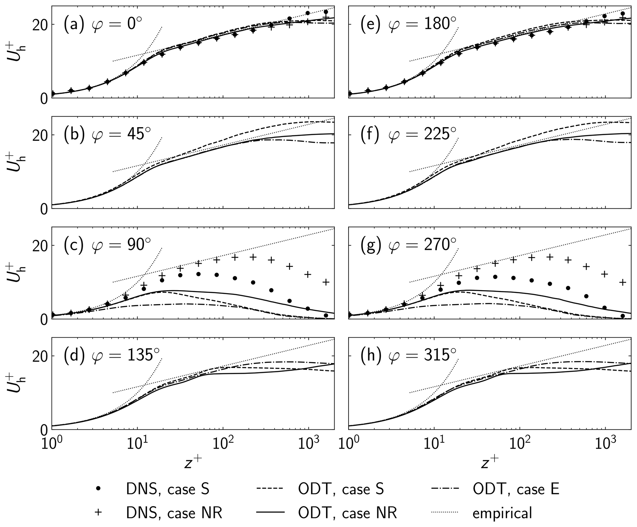
Figure 2Simulated phase-averaged law-of-the-wall plots for the horizontal velocity. The three ODT cases E, NR, and S (dashed and solid lines) as defined in Fig. 1b are compared with two available reference DNS cases NR and S (symbols) from Salon and Armenio (2011). The empirical law-of-the-wall (dotted lines) is based on the approximately collapsing reference DNS cases NR and S in panels (a) and (e), which is tangent to the DNS case NR in panels (c) and (g). The law-of-the-wall is parameterized as $U_{\mathrm{h}}^{+}=z^{+}$ for $z^{+}<\mathrm{5}$, and $U_{\mathrm{h}}^{+}={\mathit{\kappa }}^{-\mathrm{1}}\ln z^{+}+A$ for $z^{+}>\mathrm{20}$ with the von Kármán constant κ=0.41 and the additive constant A=6.0.

Download

Long-time ODT simulations with statistical gathering over N=1000 forcing periods have been conducted for eight equispaced ($\mathrm{\Delta }\mathit{\phi }=\mathrm{45}{}^{\circ }$) phases φ. Equation (6) yields an N ensemble of momentary flow profiles for each selected phase. The phase averaging follows Salon and Armenio (2011) and Ghasemi et al. (2018) for the horizontal velocity components u and v with the only difference that the wall oscillation needs to be compensated in the present case. This yields the phase-averaged velocity components 〈u〉 and 〈v〉 as ensemble average over all times t_n that belong to the stationary phase φ such that

$$\begin{array}{}\text{(8)}& {\displaystyle }\langle u\rangle \left(z\right)={\displaystyle \frac{\mathrm{1}}{N}}\sum _{n=\mathrm{1}}^{N}u(z,t_n)-U\cos \left(\mathit{\phi }\right),\text{(9)}& {\displaystyle }\langle v\rangle \left(z\right)={\displaystyle \frac{\mathrm{1}}{N}}\sum _{n=\mathrm{1}}^{N}v(z,t_n),\end{array}$$

which can be combined to yield the phase-averaged horizontal velocity profile U_h(z) through

$$\begin{array}{}\text{(10)}& U_{\mathrm{h}}=\sqrt{\langle u{\rangle }^{\mathrm{2}}+\langle v{\rangle }^{\mathrm{2}}}.\end{array}$$

The friction velocity U_⋆ and the viscous length scale δ_ν are in turn obtained from the vertical gradient of U_h(z) evaluated at z=0 as

$$\begin{array}{}\text{(11)}& {\displaystyle }{U}_{\star }=\sqrt{\mathit{\nu }{\left.{\displaystyle \frac{\mathrm{d}{U}_{\mathrm{h}}}{\mathrm{d}z}}\right|}_{z=\mathrm{0}}},\text{(12)}& {\displaystyle }{\mathit{\delta }}_{\star }={\displaystyle \frac{\mathit{\nu }}{U_{\star }}}.\end{array}$$

The normalized horizontal velocity profile $U^{+}\left(z^{+}\right)$ is then obtained from

$$\begin{array}{}\text{(13)}& {\displaystyle }{U}_{\mathrm{h}}^{+}={\displaystyle \frac{U_{\mathrm{h}}}{U_{\star }}},\text{(14)}& {\displaystyle }{z}^{+}={\displaystyle \frac{z}{{\mathit{\delta }}_{\mathit{\nu }}}},\end{array}$$

which is shown in Fig. 2 together with available reference DNS (Salon and Armenio, 2011). The DNS has been conducted for about two times larger Reynolds numbers, Re=1750 for case NR (σ=0.955) and Re=2090 for case S (σ=1.361). The ODT prediction captures salient features of the reference data, in particular, the statistical symmetry between the first half-period ($\mathrm{0}{}^{\circ }\le \mathit{\phi }<\mathrm{180}{}^{\circ }$) and the second half-period ($\mathrm{180}{}^{\circ }\le \mathit{\phi }<\mathrm{360}{}^{\circ }$). In addition, for φ=0 and 180^∘ the law-of-the-wall profiles are in very good agreement with the available reference data. Likewise, a qualitatively similar increase of the turbulent boundary layer thickness can be discerned in both DNS and ODT for the case NR in comparison to the cases E and S, respectively, for $\mathit{\phi }=\mathrm{90}{}^{\circ }$ and 270^∘. However, there is poor quantitative agreement for the latter two oscillation phases. The underprediction of $U_{\mathrm{h}}^{+}$ is in fact a manifestation of the overprediction of U_⋆, or the overprediction of the wall-shear stress for that matter.

The observed discrepancy between ODT and DNS can be attributed to an unphysical enhancement of the mixing in the near-surface region as a consequence of an overpredicted turbulent eddy event rate. This is supported by the fact that the ESBL turbulence is currently decaying such that ODT provides a larger resistance against relaminarization than DNS. Equation (5) provides means for a physical understanding of this behavior. Any length scale l for which the turnover time τ is real-valued yields generic eddy turbulence to occur in the model. Moreover, it is worth reminding that the Reynolds number of the reference DNS is about two times larger than in the present ODT which suggests a lack in turbulence kinetic energy (TKE) dissipation. The model, hence, has a physical justification to reside longer in the turbulent state that it has reached during the turbulence generating oscillation phase. A detailed discussion of the TKE dissipation is omitted here since it is a well-documented modeling error that has been addressed in a number of related studies on turbulent boundary layers (Kerstein, 1999; Schmidt et al., 2003; Fragner and Schmidt, 2017; Klein et al., 2022; Klein and Schmidt, 2022). This provides further support for the interpretation.

Despite these shortcomings of the standalone model formulation, it is remarkable that a simple one-dimensional model is able to capture salient dynamical features of the turbulent ESBL. Present results demonstrate that the model exhibts dynamical complexity that emerges from its construction and provides predictive capabilities. The demonstration of this previously assumed model property consolidates the transient LES-ODT predictions of Freire (2022), in which ODT provides means to mitigate the delayed development of the convective instability otherwise seen in LES-MOST that utilize a conventional surface parameterization scheme. The triggering of instability exemplifies why it is sometimes crucial to resolve small-scale processes in order to be able to accurately predict a rapid change of the atmospheric boundary layer flow.

4.2 Eddy event sequences and phase-conditioned eddy event rate

Figure 3a–c shows space-time sequences of the stochastically sampled ODT eddy events using black vertical line intervals. Eddy events occur instantaneously, covering a selected size-l interval $[z_{\mathrm{0}},z_{\mathrm{0}}+l]$. Only three forcing periods after a warm-up phase of two forcing periods are shown here. The simulated time sequence is much longer and also the vertical domain height is much larger than in the truncated plot. The eddy rate decrease with the forcing frequency which can be inferred from the sparser patterns in Fig. 3b, c when compared to Fig. 3a. Further discussion is given below after the introduction of the eddy event rate.

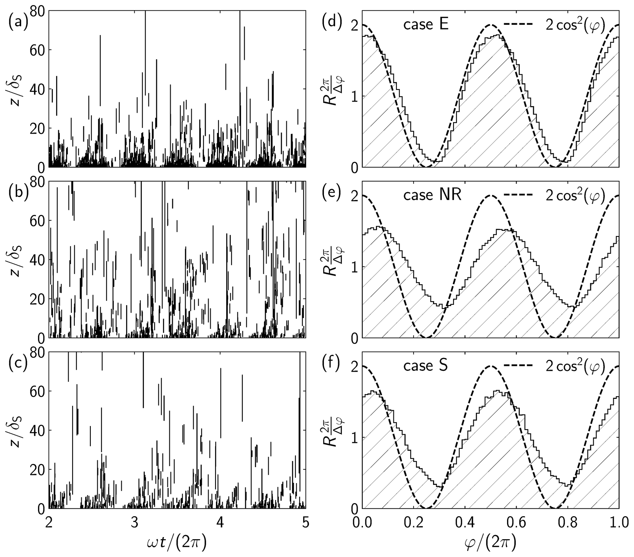
Figure 3(a–c) Vertically and temporally truncated visualization of simulated ODT eddy event sequences for the cases E, NR, and S as defined in Fig. 1b. Eddy events occur instantaneously at sampled times t_e, covering a stochastically sampled vertical interval $[z_{\mathrm{0}},z_{\mathrm{0}}+l]$. (d–f) Phase-conditioned mean eddy event rate normalized by the global rate for the cases E, NR, and S. The expected eddy event rate in the limit of quasi-static forcing (σ→0) is given for orientation (dashed line).

Download

In order to separate turbulence in different phases in response to the forcing, a phase-conditioned mean eddy event rate r(φ) can be obtained by counting the eddy events across a simulated time interval, but separately for $m=\mathrm{1},\mathrm{2},\mathrm{\dots },N_{\mathit{\phi }}$ equispaced phase intervals of size ${\mathit{\phi }}_m-{\mathit{\phi }}_{m-\mathrm{1}}=\mathrm{\Delta }\mathit{\phi }=\mathrm{2}\mathit{\pi }/N_{\mathit{\phi }}$. The total eddy event rate $r_{\text{tot}}={\sum }_{m}r\left({\mathit{\phi }}_m\right)$ is given by the sum of all individual phase-conditioned mean event rates r(φ_m). Compensating the increase of the number of eddy events per forcing period yields the phase-conditioned relative eddy event rate for any selected phase φ as

$$\begin{array}{}\text{(15)}& R\left(\mathit{\phi }\right)={\displaystyle \frac{r\left(\mathit{\phi }\right)}{r_{\text{tot}}}}.\end{array}$$

It is worth noting that R(φ) is related to the phase-conditioned posterior eddy PDF by the scaling factor $\mathrm{2}\mathit{\pi }/\mathrm{\Delta }\mathit{\phi }$. So, for any fixed phase, the information in R is the same as in the posterior eddy PDF.

Figure 3d–f shows the phase-conditioned relative mean eddy event rate in PDF normalization for an N=1000 ensemble of simulated forcing periods for N_φ=90 bins in a forcing period so that $\mathrm{\Delta }\mathit{\phi }=\mathrm{4}{}^{\circ }$. All phase-conditioned eddy event rates shown are invariant to phase rotations by integer multiples of π due to mirror symmetry in the forcing for a planar surface. The expectation for the limiting case of quasi-steady forcing (σ→0) also exhibits this symmetry and is given for orientation since turbulence modulations would follow the wall oscillation exactly. For low forcing frequencies (case E), the eddy event sequence is almost quasi-statically tied to the forcing and the turbulence activity is localized near the wall. Note that the eddy events do not actually intersect the surface, but can reach arbitrarily close to it, which is the model analog of the attached-eddy phenomenology (Townsend, 1976). For the near-resonant (case NR), turbulence reaches up high above the surface (and even higher than shown here). This qualitative result can be interpreted as a sudden increase of the bulk–surface coupling. The origin of the effect lies in the “eruption” of the laminar boundary layer thickness δ₋ as shown in Fig. 1b. The time-dependent velocity shear reaches up high above the surface due to the laminar response of the ESBL. Detached turbulence can hence be effectively driven by relative horizontal wall oscillations. This can be interpreted as dynamical enhancement of the bulk–surface coupling in rotating boundary layers. The phase-conditioned eddy event rate shown exhibits a phase lag relative to the prescribed wall oscillation. This can be attributed to the interplay of the Ekman and Stokes properties of the ESBL which leads to phase lagged dynamics with increasing distance from the surface (Thorade, 1928; Salon and Armenio, 2011; Ghasemi et al., 2018), which is captured to at least leading order by the model (Klein and Schmidt, 2020).

At a large forcing frequency (case S), the phase-conditioned eddy event rate has developed into a less uniform distribution than in the case NR. This is due to less eddy event occurrences due to a reduction of the forcing period which leaves less time for turbulence evolution (Ghasemi et al., 2018). These effects reflect the reduction of the laminar Stokes boundary layer thickness with increasing forcing frequency, that is, ${\mathit{\delta }}_{\text{S}}\propto {\mathit{\sigma }}^{-\mathrm{1}/\mathrm{2}}$ (see Fig. 1b). Due to the fixed amplitude of the utilized wall forcing, the wall-shear stress increases as velocity gradients are more localized at the surface as δ_S reduces. Together with the decreasing forcing period, $\mathrm{2}\mathit{\pi }/{\mathit{\sigma }}^{-\mathrm{1}}$, there is less time and less near-wall fluid affected by the forcing which hinders the development of an extended turbulent boundary layer. Correspondingly, fewer eddy events occur per wall oscillation period as the forcing frequency increases as demonstrated in Fig. 3a–c. Some detached residual turbulence can be observed despite the reduction of the total eddy event rate r_tot. The residual turbulence is decoupled from the surface hinting at a weakening of the bulk–surface coupling when forcing frequencies are significantly larger than the local Coriolis parameter.

The model results demonstrate that additional physical information can be extracted from ODT eddy event sequences as these are a simulation result. In fact, the spatio-temporal density of eddy events can be viewed as a turbulence indicator that provides a simple (“bare-bone”) representation of turbulence activity. Such information cannot be obtained from closure-based single-column models. Only DNS or high-resolution LES can provide similar dynamical details, for instance, in terms of the Bradshaw number as used by Salon and Armenio (2011). This, however, requires full information about the vorticity vector which is not available in the ODT.

A “minimal” version of the fully adaptive ODT implementation used for this study is publicly available at the URL https://github.com/ElsevierSoftwareX/SOFTX-D-20-00063 (last access: 23 June 2023), which is the permanent link as published in Stephens and Lignell (2021). All reference data was published previously and is publicly available under the cited references. The numerical simulation data that supports the research results is available at https://doi.org/10.5281/zenodo.8022114 (Klein, 2023).

MK wrote the paper, conceptualized the research, designed the numerical experiments, conducted the numerical simulations, and analyzed the data. HS supervised the research, contributed to the conceptualization, and reviewed and edited the manuscript.

The contact author has declared that neither of the authors has any competing interests.

The publicly available version of the fully adaptive ODT code (see above) is a “minimal” version and provided “as-is” without warranty. The code version used for generation of present results is not yet publicly available, but it is a derivative of the public code that has been extended by Coriolis forces and a buoyant Boussinesq scalar (potential temperature) following Kerstein and Wunsch (2006); Klein and Schmidt (2022).

Publisher’s note: Copernicus Publications remains neutral with regard to jurisdictional claims in published maps and institutional affiliations.

This article is part of the special issue “EMS Annual Meeting: European Conference for Applied Meteorology and Climatology 2022”. It is a result of the EMS Annual Meeting: European Conference for Applied Meteorology and Climatology 2022, Bonn, Germany, 4-9 September 2022. The corresponding presentation was part of session UP1.2: Atmospheric boundary-layer processes and turbulence.

This research has been supported by the Bundesministerium für Bildung und Forschung (grant nos. 85056897 and 03SF0693A) and the Brandenburgische Technische Universität Cottbus-Senftenberg (Graduate Research School (Conference Travel Grant)).

This paper was edited by Carlos Román-Cascón and reviewed by two anonymous referees.