2.1 MoMuCAMS payload characteristics

MoMuCAMS is a modular aerosol and trace gas measurement platform designed to be flown under a tethered balloon, while it can also be operated from other “tethers” (ropes) such as from cranes or alongside towers and tall buildings. The novelty of this platform lies in its flexibility to accommodate various combinations of instruments within the weight and dimension limits. A list of instruments, which MoMuCAMS typically carries, is presented in Table 1. Examples of different instrumental combinations with respective scientific objectives are presented in Sect. 4. Importantly, MoMuCAMS can easily be adapted for additional instruments.

Table 1List of instruments available on MoMuCAMS. T: temperature, RH: relative humidity, P: barometric pressure, WS: wind speed, WD: wind direction.

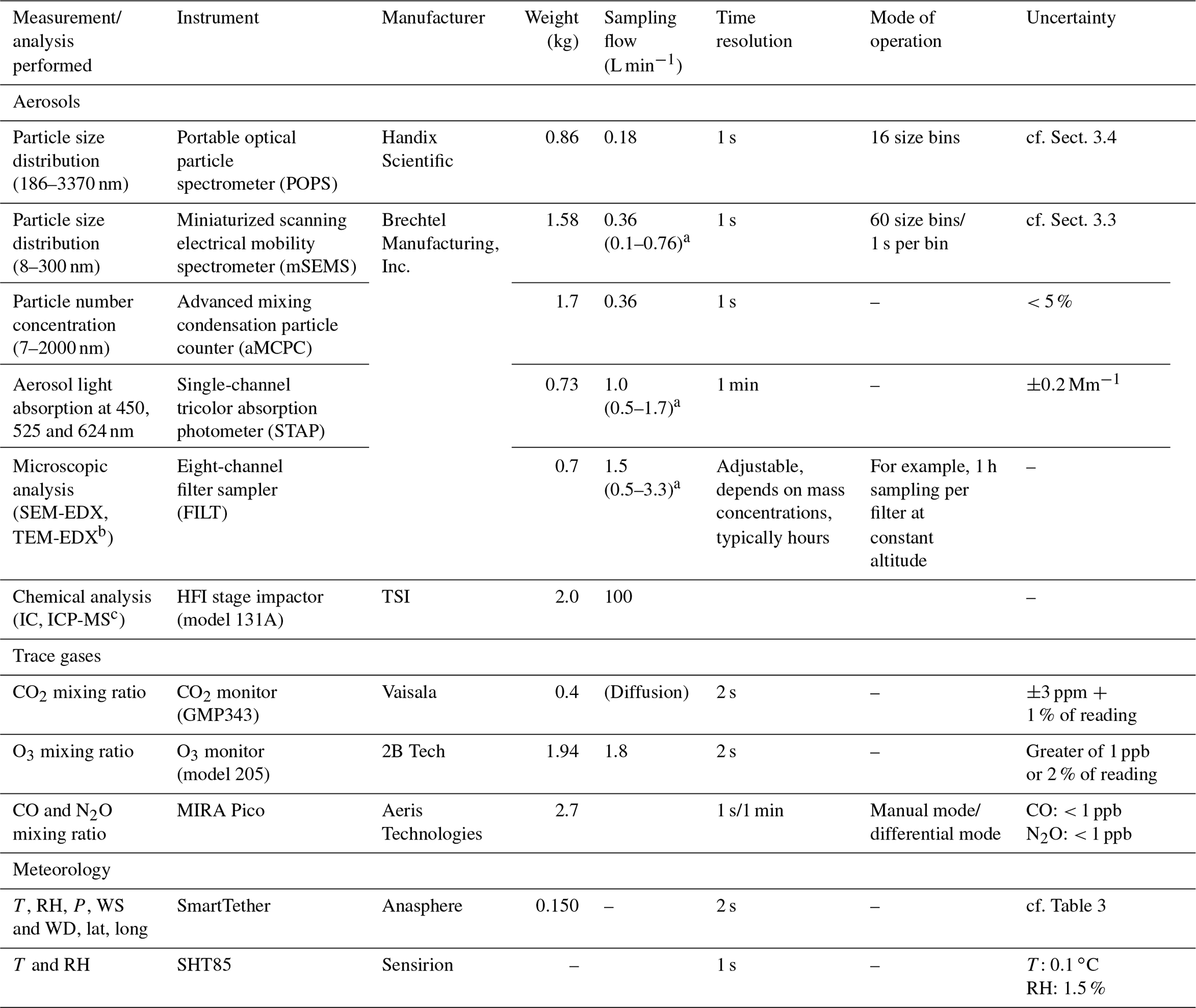
^a Values in parentheses represent the range of possible sampling flows, while the single value indicates the typical flow set during operations. ^b SEM-EDX: scanning electron microscopy with energy dispersive X-ray analysis, TEM-EDX: transmission electron microscopy with energy dispersive X-ray analysis (the analysis is done in laboratory after the flights). ^c IC: ion chromatography, ICP-MS: inductively coupled plasma mass spectrometry (the analysis is done in laboratory after the flights).

Download Print Version | Download XLSX

The payload enclosure is a box with outer dimensions of 80 × 40 × 35 cm and a cone-shaped nose on the front (see Fig. 1). It provides a total inner volume of roughly 100 L for instruments and batteries, which can be placed on two levels (“shelves”) or attached on the outside. The box is made of 30 mm thick extruded polystyrene plates. This material was selected for its low weight, rigidity and thermal insulation properties. Two aluminum T elements placed at the front and back of the box support the enclosure from underneath and are used to attach it to the balloon. This system guarantees the stability of the payload in the air. The box weighs (including the power distribution system and aluminum reinforcements) 3.2 kg. The instruments are powered by lithium-polymer (LiPo) batteries. Batteries with a capacity between 9 and 22 A h and a nominal voltage of 22.2 V are typically used. The maximum flight operation time will depend on the selected batteries, instrumental setup and ambient air temperature but usually ranges from 2 to 10 h. The system is equipped with two 20 W resistive heaters connected to a thermostat to ensure the inner environment of the box remains above 0 ^∘C.

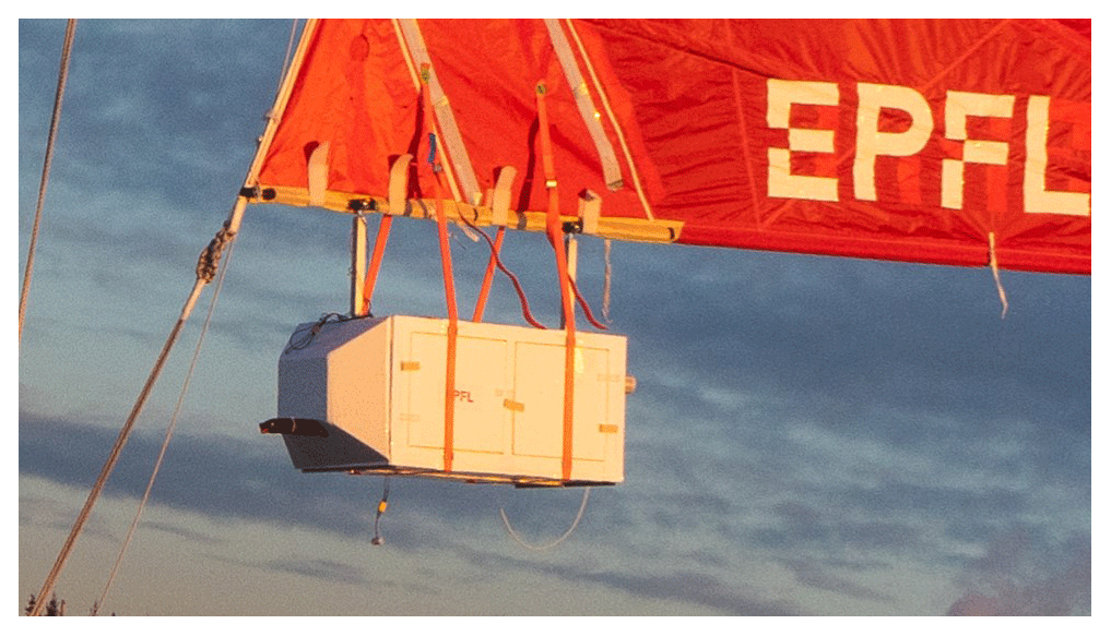
Figure 1Picture of the MoMuCAMS payload attached to the Helikite. Two aluminum bars connected directly to the Helikite's structure ensure stability of the payload. Two additional cargo straps provide additional safety for the payload attachment. The system remains very stable, even at winds above 15 m s⁻¹.

Download

A custom-made data-logging and communication system has been designed for MoMuCAMS. A Teensy 3.6 microcontroller programmed with Arduino IDE (integrated development environment) controls the different tasks. The microcontroller saves data from onboard sensors measuring the internal temperature, barometric pressure, external and sampled air temperature and relative humidity, battery state of charge, particle number concentration from an optical particle counter, and CO₂ mixing ratio. Data are also simultaneously transmitted to the ground through an XBee 3.0 radio module.

Figure 2 shows a schematic sketch of the inner design. The data are visualized live on a graphical interface, which helps with decision-making and sampling strategy adaptation during flights. Additionally, the operator can use the graphical interface to send commands to the MoMuCAMS microcontroller. Commands include activation and filter position change of an eight-channel filter sampler for microscopy analysis (FILT), the activation and flow control of a high-flow impactor (HFI), the activation of a relay to power additional instruments at a desired altitude, and the general shutdown of the system.

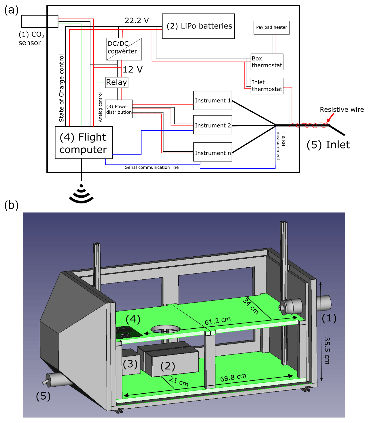
Figure 2(a) Schematic of the MoMuCAMS design. Black and red paths represent power wires. Blue and green lines represent serial and analog communication connections for communication between different instruments/components and the flight computer. The setup is flexible and can accommodate different aerosol and trace gas instruments; thus the layout of instruments is only illustrative. (b) 3D drawing of the MoMuCAMS enclosure without side panels and top cover. Green surfaces represent available space for instrumentation. Numbered elements are introduced in panel (a).

Download

2.2 Helikite

A Helikite (Desert Star, Allsopp Helikites, UK) has been used to lift the payload. The balloon consists of an outer shell and an inner membrane, which contains the helium. A Helikite combines the lifting capacity from the helium and from a kite, providing higher lift and good stability in windy conditions. The lifting capability of the Helikite depends on the takeoff altitude, i.e., atmospheric pressure, and wind speed. The Helikite used for this study has a volume of 45 m³ and a tether length of 800 m (combined in two winches with 400 m of rope each). It is usually sufficient to lift a payload between 12 and 20 kg. The Helikite has been selected for its rugged characteristics, which allow for deployments in the harsh environmental conditions of polar and mountain regions. The Helikite–MoMuCAMS setup has successfully flown at wind speeds up to 15 m s⁻¹, in temperatures down to −36 ^∘C and in clouds (see Fig. S2 in the Supplement). Note that when the air reaches very low temperatures (we estimate that −20 ^∘C represents a critical threshold), small punctures form in the balloon's inner membrane, which will consequently lead to helium losses over time and reduced operation time (the inner membrane has to be repaired or replaced). As wind increases, the zenith angle of the line increases as well, reducing the maximum altitude reachable with the Helikite. The angle depends on not only the wind speed but also the net lift of the Helikite, which will depend on the atmospheric pressure, inflation state of the balloon, presence of water, weight of the payload and tether. Estimates of zenith angles have been calculated from the horizontal displacement of the Helikite (measured by GPS) and its altitude above ground level. Figure S3 shows results for two fields campaigns. Generally, the zenith angle tends to stabilize between 45 and 50^∘ at around 8 to 10 m s⁻¹, which corresponds to a maximum altitude between 515 and 565 m a.g.l. (above ground level) for an 800 m long tether. While in this paper we focus on the system built for a 45 m³ Helikite with an 800 m tether, MoMuCAMS is independent from the lifting platform and can be used with a larger balloon and longer tether to reach higher altitudes.

3.1 Inlet sampling efficiency and transmission losses

The inlet system is composed of a horizontal 30 cm long $\mathrm{3}/\mathrm{8}$ in. (9.525 mm) stainless-steel tube at the front of the box. Because the tethered balloon orients with the wind, the inlet is always facing into the wind direction. The tip of the inlet has a 30^∘ downward bend to prevent water droplets from entering. Careful inspection of the inlet after each flight has not shown any signs of water infiltration in the sampling line. A flexible thermofoil around the inlet heats the sample flow to reduce relative humidity to < 40 %, which corresponds to Global Atmosphere Watch standards (World Meteorological Organization, 2016) and prevents ice formation when sampling in cold environments (see Fig. S2c). The inlet heating is controlled by a miniaturized thermostat (CT325, Minco) and set to be always above 0 or ∼ 10 ^∘C higher if ambient temperature is positive. Sample air temperature and relative humidity are monitored by a sensor (SHT80, Sensirion, Switzerland). The sensor is placed inside the sampling line in parallel to the instruments to avoid particle losses. The sampled air is split into $\mathrm{1}/\mathrm{4}$ in. (6.35 mm) branches, and conductive black silicon tubing distributes the sampled air to the different instruments. Additionally, gas sensors such as the ozone monitor and the stage impactor have their own inlet made of Teflon and Tygon, respectively. The carbon dioxide sensor is installed on the outside of the box and measures air flowing through passively.

The overall sampling performance of the main inlet has been characterized both experimentally and with the Particle Loss Calculator (PLC) (von der Weiden et al., 2009). Sampling efficiency (see Fig. 3) has been computed for wind speeds between 0 and 10 m s⁻¹, representative of most operating conditions, and a total sampling flow of 1.72 L min⁻¹, which is representative of a typical instrumental setup installed on MoMuCAMS. The flow rate may slightly vary from one setup to another. Results from the PLC indicate that oversampling, due to super-kinetic conditions, becomes important only for larger particles (> 2 µm) at higher wind speeds.

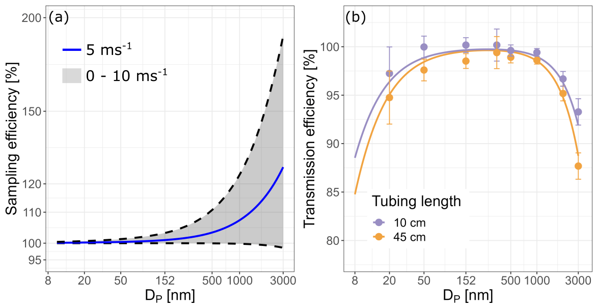
Figure 3(a) Inlet sampling efficiency at 1.72 L min⁻¹ sampling flow. The shaded area represents wind speeds between 0 and 10 m s⁻¹. The blue line represents the sampling efficiency at 5 m s⁻¹. (b) Inlet transmission results from experimental tests and the PLC. Each dot represents a 5 min average of transmission efficiency measurements, and the error bars represent the standard deviation. The two lines are results obtained from the PLC. Colors indicate the length of the black tubing connecting the end of the stainless-steel inlet to the CPC and represent the range of line lengths inside MoMuCAMS.

Download

Transmission losses in the inlet have been experimentally tested with particles of different diameters (D_p). For particles up to 350 nm, polystyrene latex spheres (PSLs) were nebulized and dried through a silica gel column (similar to the TSI 3062 type). The size selection was then refined with a differential mobility analyzer (DMA). For particles larger than 350 nm, a di-ethyl-hexyl-sebacat (DEHS) solution was used to produce particles. After that nebulization particles were dried and size-selected with an aerodynamic aerosol classifier (AAC, Cambustion, UK). The aerodynamic diameter was later converted to mobility diameter for a more coherent comparison with the small particles selected with a DMA. A reference condensation particle counter (CPC) measured the particle number concentration after the DMA and AAC, while two CPCs were placed after the inlet. To represent the different tubing lengths inside the payload, one CPC was placed behind a short piece of black tubing (10 cm) and one was placed behind a longer piece (45 cm). The total flow through the main inlet was 1.72 L min⁻¹. Before the experiment, all CPCs were connected in parallel for direct comparison. Results from the CPC intercomparison are presented in Sect. 3.2. Figure 3b shows the results of the inlet transmission test (colored dots with error bars) for eight different particles diameters and from the PLC for particles ranging from 8 to 3000 nm. Generally, results compare well between the experiment and the PLC with slightly lower losses for the shorter inlet. Transmission efficiency for particles between 50 and 1000 nm is very close to 100 %, while smaller particles suffer from diffusional losses and larger particles suffer from gravitational deposition. However, the losses are typically less than 10 %.

3.2 Advanced mixing condensation particle counter (aMCPC)

The compact advanced mixing condensation particle counter (aMCPC, model 9403, Brechtel Manufacturing, Inc., USA) is used for total particle number concentration measurements from 7 to 2000 nm and weighs 1.7 kg. Two aMCPCs have been compared against a reference MCPC with the same measurement range (MCPC, model 1720, Brechtel Manufacturing, Inc., USA) with PSLs of D_p 150 nm. PSLs were nebulized and dried as described in Sect. 3.1. The two aMCPCs and the reference MCPC were connected in parallel behind the drier. Figure S4 shows results of the experiment. Both aMCPCs agree well (within 5 %) with the reference MCPC.

In addition, the d₅₀ cutoff (defined as the diameter where the counting efficiency reaches 50 %) of both aMCPCs was tested experimentally by comparing the measured concentration of the aMCPCs and a reference ultrafine CPC (CPC3776, TSI, USA). All three CPCs were intercompared before the d₅₀ cutoff measurements, and concentration was corrected to account for differences in the counting efficiency (they all agree within a 7 % factor). Particles were generated by nebulizing pure Milli-Q water, which produces ultrafine particles due to small impurities inherently found in both the water and the container (Knight and Petrucci, 2003; Park et al., 2012). The particles were then dried and size-selected with a DMA. The two aMCPCs and reference ultrafine CPC were then connected in parallel behind the DMA. The total aerosol flow was equal to 1.3 L min⁻¹, while the sheath flow in the DMA was set to 10 L min⁻¹. The tubing going to each CPC was the same length to ensure similar losses (approximately 20 cm long). The size selection was done in steps of 0.5 nm from 5.5 to 10 nm, with 600 s long measurements for each step. Results are shown in Fig. S5. Note that the automatic scanning sequence produced two measurements for 7 and 7.5 nm particles. For transparency, results of both measurements are shown separately in Fig. S5. The experimental results were fitted with an exponential function (Eq. 1) (Stolzenburg and McMurry, 1991).

with fit results of A= 1.05, B= 5.13 and C= 6.01 for aMCPC 21 and A= 1.02, B= 5.20 and C= 5.72 for aMCPC 22. The d₅₀ cutoff (parameter C), was found to be equal to 6 and 5.7 nm for aMCPC 21 and aMCPC 22, respectively. The detection efficiency for both aMCPCs reaches a plateau between roughly 8 and 9 nm, which is in agreement with the manufacturer's specifications.

3.3 Miniaturized scanning electrical mobility sizer (mSEMS)

The miniaturized scanning electrical mobility sizer (mSEMS, model 9404, Brechtel Manufacturing, Inc., USA) is a compact particle size spectrometer providing the particle number size distribution (PNSD) based on the mobility diameter for particles between 8 and 300 nm. The instrument is composed of a soft X-ray aerosol charge neutralizer (soft X-ray charger, XRC-05, HCTM Co., Ltd., South Korea), a miniaturized DMA (differential mobility analyzer) column and an aMCPC with a total weight of 4.4 kg. The design of the DMA has been optimized to minimize the high voltage required for particle selection and therefore reduces problems of arching at higher relative humidity or lower pressure. The small internal volumes of the DMA and inlet tubing and the fast aMCPC time response facilitate rapid scanning due to minimal smearing/mixing volumes inside the instrument.

The performance of the mSEMS was tested with different particles covering its size range. Particles smaller than 50 nm were obtained by nebulizing pure Milli-Q water using the portable aerosol generation system (PAGS, Handix Scientific, USA). After nebulization, particles were dried through a silica gel dryer and size-selected with a DMA. Particles larger than 50 nm were obtained by nebulizing PSL solutions and following the same procedure as with the pure Milli-Q. For each size, particles were nebulized for over 10 min to allow for enough scans to be counted. The mSEMS was set to 60 bins at 1 s per bin. The mobility diameter (D_mob) was obtained by fitting a lognormal distribution to the measured PNSD and taking the peak value (mean). Results of the experiments are presented in Fig. 4a and Table 2. Overall, deviation in particle sizing, i.e., the relative difference between the particle size (D_p) and the measured distribution peak (D_mob), is below 7 %.

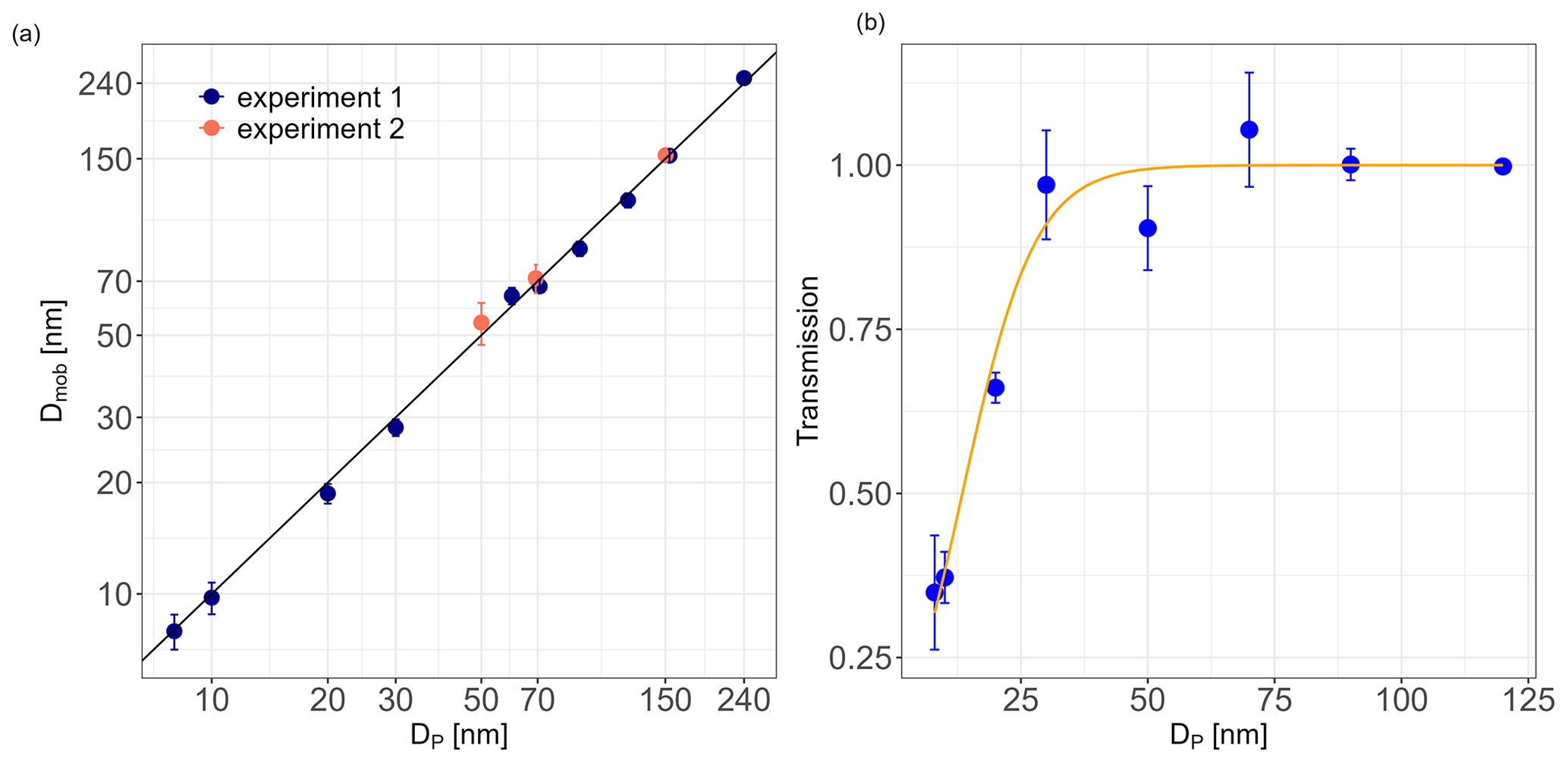
Figure 4(a) Measured particle mobility diameter (D_mob) from a lognormal fit of the measured PNSD from the mSEMS against the diameter of reference PSLs or impurities from nebulized Milli-Q water. The black line represents equal diameters of reference particles and measured D_mob. The experiment was conducted on two separate occasions (experiments 1 and 2). Error bars indicate the standard deviation of the lognormal distribution fitted to the mSEMS measurement. (b) Particle transmission through the DMA. Error bars indicate the standard deviation of the period of comparison (15 min). The orange curve represents the best fit of the theoretical transmission function (Eq. 1).

Download

Table 2Results of mSEMS performance. D_mob indicates the peak of the fitted lognormal distribution for the respective particle diameter (D_p). σ represents the standard deviation of fitted distribution, and $\left|{\mathrm{\Delta }}_{D_{\mathrm{mob}}-D_{\mathrm{p}}}\right|$ represents the absolute deviation in percent between D_mob and D_p.

Download Print Version | Download XLSX

In addition, particle transmission through the neutralizer and DMA has been tested for different particle sizes. For the experiment, particles were nebulized and size-selected with a first DMA. A standalone aMCPC was connected in parallel to the mSEMS after the first DMA. Transmission through the mSEMS (neutralizer and DMA) was calculated by comparing the particle number concentration measured by the two aMCPCs. Results are presented in Fig. 4b. The sinusoidal function is (Eq. 2)

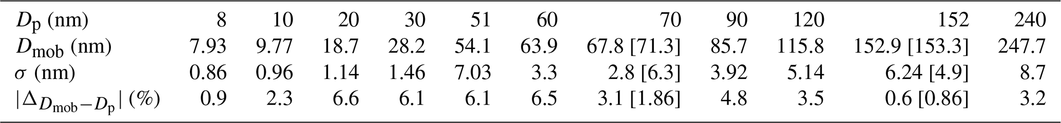
with fit results of A= 1.00, B= 0.14 and x₀= 13.46, where x₀ is the 50 % transmission point that was used to fit the experimental transmission results. Based on the measured losses below 30 nm, a correction is applied to the mSEMS data obtained in the field using Eq. (2). Figure 5 shows results of 10 min averaged integrated particle number concentrations from the mSEMS against a standalone aMCPC measuring in parallel. Data were collected from a ground measurement station in Brigerbad, Switzerland, between 8 and 11 October 2021 (see Sect. 4.2 for campaign details). Figure 5a shows results for the original mSEMS data, and Fig. 5b shows results after data correction. The color scale indicates the number concentration (N₈₋₃₀) of particles with D_mob between 8 and 30 nm to highlight the higher discrepancies between the mSEMS and the aMCPC when the number of ultrafine particles increases. Dots indicating higher N₈₋₃₀ are typically further away from the 1:1 line (Fig. 5a), confirming an underestimation of total number concentration because of ultrafine particle losses through the neutralizer and DMA. By applying the empirical transmission loss correction function, the slope of the linear regression increases from 0.61 to 0.79 and the scatter in the data is reduced (R² increases from 0.94 to 0.99, Fig. 5b). The remaining underestimation of the particle concentration can be explained by the narrower size range counted by the mSEMS (8 to 280 nm) compared to the aMCPC (7 to 2000 nm). These measurements show that ultrafine particle losses in the mSEMS are non-negligible and a correction factor should be applied to improve measurement accuracy.

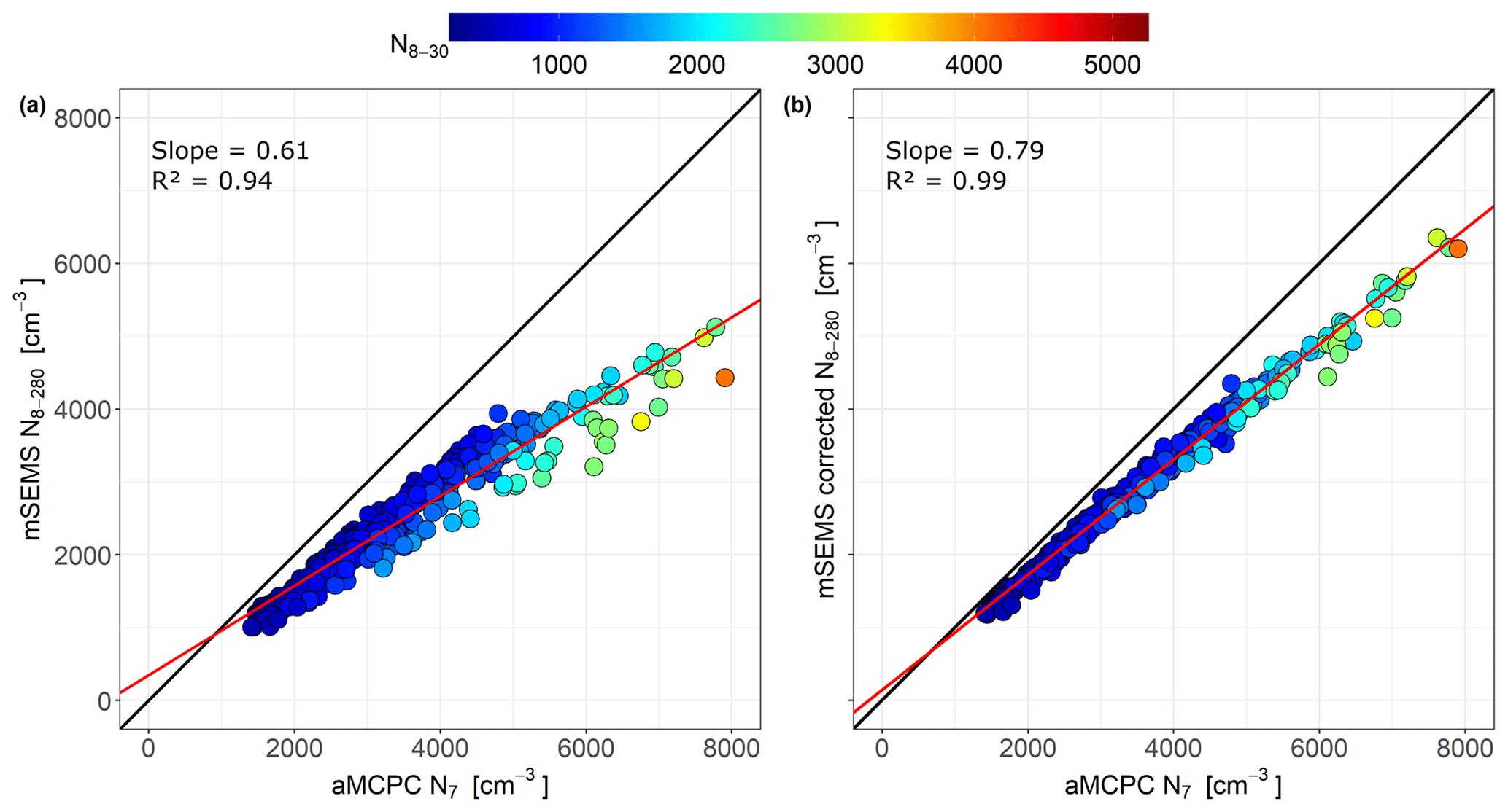
Figure 5Scatterplots of the 10 min averaged particle number concentration. Panel (a) shows concentration from the aMCPC (x axis) against the integrated measured concentration from the mSEMS (y axis). Panel (b) shows the same but with corrected mSEMS data. The color scale indicates the total concentration of particles between 8 and 30 nm.

Download

In this study, the instrument is operated at a 0.36 L min⁻¹ sample flow and 2.5 L min⁻¹ sheath flow. The selected size range is from 8 to 280 nm with 60 bins and a scan time of 1 min (up-scan). Note that the given values may need to be adjusted for environments with very low particle number concentrations (i.e., < 100 cm⁻³) to ensure good counting statistics, similarly to an electrical mobility sizer. Comparison of up- versus down-scan performance of the mSEMS has shown no significant difference between the two modes. Results of a 6 h averaged PNSD for up- and down-scans is shown in Fig. S8.

3.4 Portable optical particle spectrometer (POPS)

The well-characterized portable optical particle spectrometer (POPS, Handix Scientific, USA) is used to obtain PNSD and number concentrations of particles between 186 and 3370 nm (Gao et al., 2016; Mei et al., 2020; Liu et al., 2021).

Sizing calibration of two POPSs (one for flights, POPS 105; one for ground measurements, POPS 101) was performed with polystyrene latex spheres (PSLs) of sizes 240, 500, 800 and 994 nm. Nebulized particles passed inside a silica gel dryer to remove water. A 200-bin size segregation was used to improve the resolution of the size distribution around the main particle size mode. For each PSL diameter, the POPS measured for 5 min once the concentration became stable. Figure S6 shows results from measured optical diameters (D_OPT) calculated from lognormal fits of averaged PNSDs. The uncertainty (error bars) is represented by 1 standard deviation of the fitted function. POPS 105 shows deviations below 10 % for PSLs up to 800 nm, while POPS 101 shows slightly higher deviations up to 20 % for 500 nm particles. Both POPSs show higher deviation for 994 nm particles, i.e., 34 % and 29 % for POPS 101 and POPS 105, respectively. The higher deviation for particles around 1 µm can be explained by Mie resonance in this size range and has also been observed by Pilz et al. (2022). We therefore follow their recommendations by setting the POPS size resolution to 16 log-spaced bins to minimize sizing errors. Note that the sizing characterization was performed with PSLs with a refractive index of 1.59. The refractive index of tropospheric aerosol particles typically is in the 1.50–1.55 range (Aldhaif et al., 2018), which is close enough to that of PSLs to only have a minor effect on the sizing accuracy of the POPS (Mei et al., 2020). However, if measurements were to be conducted in environments with aerosols having markedly different optical properties – for example, in arid regions with a high concentration of mineral dust – the data could be significantly affected and should be treated accordingly.

Counting efficiency of the two POPSs was tested against the reference mixing condensation particle counter (MCPC, model 1720, Brechtel Manufacturing, Inc.). PSLs with a diameter of 230 nm were nebulized, dried and further size-selected with a DMA. Background noise of the POPS was tested with particle-free air. Both the POPS and the reference CPC showed a concentration of 0 cm⁻³. PSLs were then nebulized into the inlet. Concentrations were incrementally increased by modifying the particle-to-air ratio of the nebulizer. Figure S7 shows results of particle number concentrations of the two POPSs against the reference CPC including all 16 bins (142–3370 nm, dots) and bins 4 to 16 (186–3370 nm, triangles). Results from Fig. S7 indicate that the measurements of particles with diameters less than 186 nm (bins 1 to 3) are affected by measurement artifacts that result in inflated apparent particle counts that scaled with particle concentration.

This phenomenon, potentially associated with stray light in the optics chamber, was already reported in previous literature (Gao et al., 2016; Mei et al., 2020; Pilz et al., 2022). According to the manufacturer, these wrong detections could also be explained by electronic noise from the detector, where fringes on the edge of the Gaussian signal are perceived as smaller particles by the software. It was therefore decided to only consider data for particles larger than 186 nm as the error induced by the first three bins is too high. Overall, both POPSs show very good agreement with the reference CPC with a deviation below 10 % for the total number concentrations.

3.5 Comparison of the mSEMS and POPS

To assess the comparability of the mSEMS and POPS measurements, the instruments have been installed in parallel with a scanning electrical mobility spectrometer (SEMS, model 2100, Brechtel Manufacturing, Inc., USA). The mSEMS and POPS were directly connected to the same whole air inlet as the SEMS. Figure 6 shows results of the comparison between 30 and 31 January 2022. Panels a and b show comparative time series of the 10 min averaged integrated total particle number concentration between the SEMS (blue) and mSEMS (red) and between the SEMS and POPS (green), respectively. The particle size range was from 8 to 270 nm (N₈₋₂₇₀) and 180 to 1500 (N_180−1500) for panels a and b, respectively. Note that the size range of each instrument differed slightly because of respective bin limits and different types of measured diameters (i.e., mobility versus optical diameter, POPS size range for bins 4 to 14 = 186 to 1480 nm). Regression slopes of 0.98 and 0.89 confirmed good agreement between the instruments for the particle number concentration in their respective size range. Figure 6c shows PNSD from the three instruments between 02:00 and 04:00 LT on 31 January 2022 (shaded area in Fig. 6a and b). The full line represents the median PNSD, and the colored shading represents the interquartile range. Note that no conversion was made to transform the optical diameter from the POPS into the electrical mobility diameter. Given the different size ranges covered by the instruments and the several orders of magnitude of the y axis, enlargements of the PNSD are shown in the corners of the figure to better assess the comparability of the instruments. To quantify the comparability of the measurements, both the mSEMS and SEMS PNSD were fitted with a lognormal distribution. The mode peaks of the mSEMS and SEMS are 29.7 and 33 nm, respectively, yielding a 10 % difference. To compare size-dependent particle counting between the mSEMS and the SEMS, the integrated particle concentration for several diameter intervals has been calculated. Results indicate that the mSEMS tends to overestimate the number of particles below 30 nm by 30 % to 40 % compared to the SEMS. For particles larger than 30 nm, the agreement between the two instruments is well within 5 %. Detailed results for each size intervals is shown in Table S1 in the Supplement. Overall, the mSEMS and SEMS show very good agreement for total number concentration and show very comparative size distribution. For particles below 30 nm, the deviation is larger, which could potentially be attributed to difference in charging efficiency of the two neutralizers and slight differences in the inversion algorithm of the mSEMS and SEMS.

Figure 6Comparison of the mSEMS, SEMS and POPS between 30 and 31 January 2022. Measurements were performed at the University of Alaska Fairbanks farm field in Fairbanks, Alaska, USA (64^∘51^′12^′′ N, 147^∘51^′34^′′ W). (a) Time series of the particle number concentration from 8 to 280 nm (N₈₋₂₈₀) from the mSEMS (red) and SEMS (blue). (b) Time series of the particle number concentration from 180 to 1500 nm (N_180−1500) from the POPS (green) and SEMS (blue). (c) Particle number size distribution measured from 02:00 and 04:00 LT on 31 January (shaded grey area in panels a and b). The x axis represents the electrical mobility diameter (D_mob) of the SEMS and mSEMS and the optical diameter (D_OPT) of the POPS.

Download

Comparison of normalized bin concentrations between the POPS and both electrical mobility analyzers showed correspondence within 5 % between the POPS and the mSEMS for the overlapping size range. Differences between the POPS and the SEMS is up to 20 %, but overall the overlapping of the optical and mobility diameters are within the uncertainty intervals (colored shading in Fig. 6c). Note that a full evaluation of a conversion from the POPS optical diameter to electrical mobility diameter would need to be performed to fully characterize the comparativeness of these instruments.

3.6 MIRA Pico CO $/$ N₂O $/$ H₂O analyzer

The Pico (MIRA Pico CO $/$ N₂O, Aeris Technologies, USA) is a compact NDIR-based (non-dispersive infrared) gas analyzer. The instrument uses middle-infrared laser absorption spectroscopy to measure CO, the N₂O dry mole fraction and H₂O with a detection limit below the level of parts per billion. A few studies have provided information on the performance of the Pico instrument, however only for the methane (CH₄) version (Commane et al., 2022; Travis et al., 2020). This study provides a first look at in-flight operations of the CO version.

The instrument is integrated inside a small Pelican case (30 × 20 × 9 cm) and weighs 2.7 kg, including a battery with a 6 h lifetime. The Pico can work in two different modes. The instrument is equipped with two programmable sampling ports. In its differential mode, the system switches between the two sampling ports at a user-definable time interval (30 s by default). A catalytic CO scrubber is placed in front of the first port, providing a zero measurement for each interval, effectively preventing any slow instrument drift. The software automatically removes the baseline (zero measurement) from the actual measurement. In this configuration, the Pico provides measurements at a 1 min time resolution with a 1 ppb accuracy (the value is provided by the manufacturer but has not been validated experimentally). In its manual mode, the instrument samples only from one port with a 1 s time resolution. In this configuration, no baseline correction is applied to the measurements, reducing the overall accuracy. To estimate the reduction in precision due to unaccounted baseline drifts occurring over a typical flight period, we analyzed zero measurements (i.e., CO scrubber installed in front of the sampling port and Pico operating in manual mode) for 90 min. We consider 2 standard deviations of the zero measurement distribution as an upper limit estimate of the measurement uncertainty in manual mode; this value is equal to 17 ppb.

For flight operation, the manual mode is preferred to provide the highest time resolution possible. To account for the baseline, the instrument is operated on the ground between flights in its differential mode. Before each flight, the instrument is placed inside the box and brought outside until temperature inside the box has stabilized. The CO scrubber is removed, and the Pico is set to manual mode just before takeoff. The baseline measurement for the last 3 h before the flight and 3 h after the flight is then averaged and subtracted from the flight measurements. This operation should provide the best estimate for the baseline deduction from the measured values. To identify whether pressure or temperature changes have any influence on the instrument's baseline, several flights were performed in differential mode. Figure 7a shows the baseline measurement for a full campaign with color codes indicating whether the instrument was operated on the ground or in the air. Orange dots indicate that the instrument was operated inside a hut at a constant temperature of about 20 ^∘C, while blue dots are baseline measurements when the Pico was inside MoMuCAMS in flight. Figure 7b shows in more detail the baseline variability on 30 January before, during and after a flight. The recorded inner temperature of MoMuCAMS and atmospheric pressure are indicated to illustrate the lack of correlation between changing environmental conditions and the instrument's baseline.

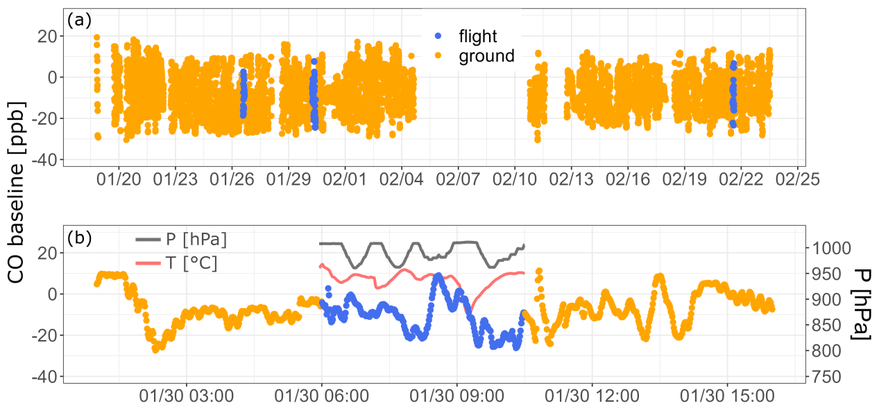
Figure 7(a) CO baseline measurements of the MIRA Pico during the ALPACA campaign from 18 January to 24 February 2022. Blue dots indicate measurements of the baseline during flights. (b) Subset of baseline measurements before, during and after a flight on 30 January 2022. The black and red lines represent the barometric pressure (right axis) and temperature inside the MoMuCAMS enclosure (left axis), respectively.

Download

Note that during measurements, we recommend saving the high-time-resolution spectral files to control good data fitting or to detect fitting issues. In the case of fitting issues, the spectral files can be processed again to correct the data.

Although we demonstrate that vertical profiling does not affect the instrument's functionality, no quantitative characterization of the Pico's performance is available besides the manufacturer's calibrations. A comparison with a reference instrument or calibration gas should be done for future quantitative assessments of CO with the Pico.

3.7 Filter sampling for chemical analyses

In addition to online measurements, the MoMuCAMS system can also be equipped with instruments for offline analysis. Two instruments are currently used to collect aerosol samples on filters for chemical and microscopic analyses. A more detailed description of the instrumental setup is given below.

A high-flow multi-stage cascade impactor (HFI, model 131A, TSI, USA) is used to collect aerosol particles on filters. Each stage is composed of multiple nozzles, achieving size selection similar to the more common micro-orifice uniform-deposit impactor (MOUDI). A nominal sampling flow of 100 L min⁻¹ is achieved by a radial flow impeller (radial blower, U85HL-024KH-4, Micronel, Switzerland) used in reverse as a lightweight pump as in Porter et al. (2020). The sampling flow is constantly monitored by a flowmeter installed in front of the blower (SFM3000, Sensirion, Switzerland). The HFI is equipped with six stages with the following cutoffs: 10, 2.5, 1.4, 1.0, 0.44 and 0.25 µm. Samples are collected for the six size cutoffs on 75 mm diameter quartz fiber filters (QR-100, 0.38 mm thickness, Advantec MFS, Inc., USA) and then on 90 mm diameter quartz fiber filters (AQFA, Merck Millipore Ltd., USA) to collect all particles below the lowest cutoff.

For more detailed information on types of analysis, filter preparation and handling, and analytical procedures, the reader is referred to the Supplement (Sect. S5).

3.8 Filter sampling for electron microscopy

An eight-channel filter sampler (FILT, model 9401, Brechtel Manufacturing, Inc., USA) is used to collect samples on substrates for electron microscopy analysis. Each channel holds a 13 mm Teflon Swinney filter holder. Polycarbonate filters with 0.4 µm pores (reference no. 321031, Milian Dutscher Group, Switzerland) are used to collect particles for scanning electron microscopy with energy dispersive X-ray analysis (SEM-EDX). Polycarbonate filters offer a smooth surface and are mechanically rugged (Genga et al., 2018; Willis and Blanchard, 2002), which is ideal for particle observation and prevents deterioration of the substrate during sampling.

For transmission electron microscopy (TEM) analysis, custom-made TEM grid holders were created to fit the standard 13 mm filter holders (see Fig. 8). Additionally, a “jetting” device (Brechtel Manufacturing, Inc., USA), placed above the grid, reduces the inlet diameter and focuses the sampling beam onto the TEM grid. The real particle impaction efficiency has however not been characterized so far.

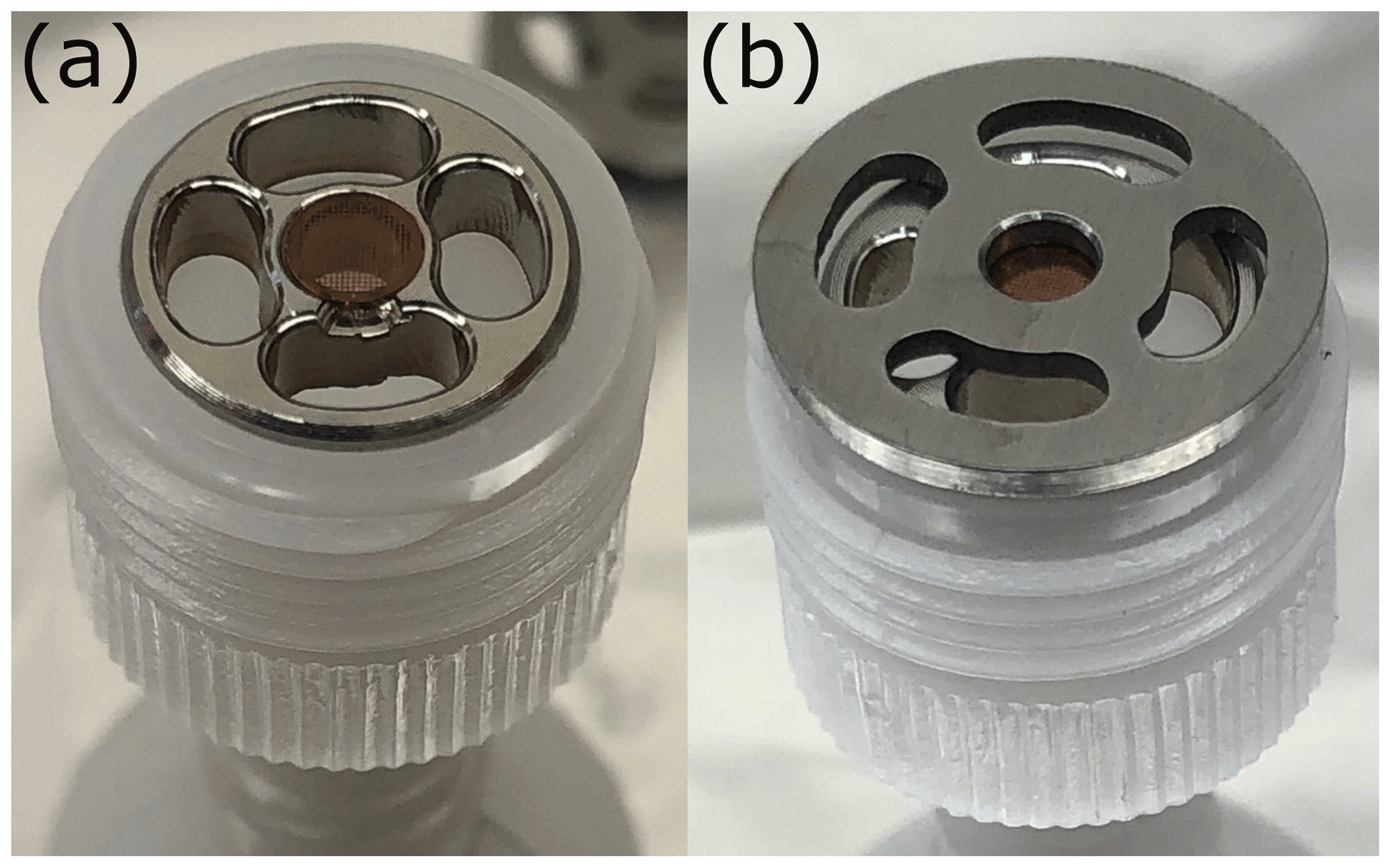
Figure 8(a) TEM grid placed on custom-made grid holder. (b) TEM grid with covering plate placed on top.

Download

The filter sampler can operate between 0.5 and 3 L min⁻¹. However, the pump does not sustain a sampling flow above 1.8 L min⁻¹ with the additional TEM grid holder and jetting device. Furthermore, higher sampling flows tend to destroy the grid's carbon membrane. Therefore, we operated the FILT with a sampling flow of 1.5 L min⁻¹. Both the sample flow and the sampling stage can be remotely controlled from the ground. After filter retrieval, filters are stored at −20 ^∘C until analysis. Airborne sampling was first performed in October 2021, in a Swiss Alpine valley. Details of electron microscopy analysis and examples of collected aerosol particles with SEM-EDX and TEM are presented in the Supplement (Sect. S.6).

3.9 Meteorological measurements

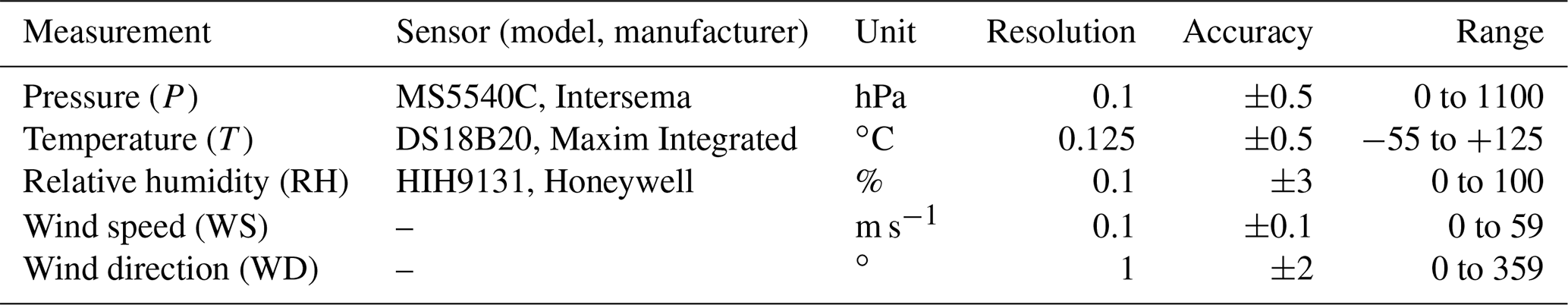
Meteorological parameters including temperature (T), relative humidity (RH), barometric pressure (P), wind speed (WS) and wind direction (WD) are measured by a lightweight sonde (SmartTether, Anasphere, USA) placed below the payload. The SmartTether is contained in a compact plastic casing mounted on a carbon fiber arrow-shaped structure. A cup anemometer is placed at the front of the structure, and a dart-like tail helps the sonde orient itself into the wind. Table 3 summarizes all measurements and the respective resolution, accuracy and operating range as provided by the manufacturer. During flight, data are transmitted to the ground and directly saved on the ground computer. Note that no data are saved locally, and in the case of communication loss, data are not saved. Furthermore, it appears that the SmartTether is sensitive to electromagnetic interferences, and frequent loss of communication was experienced in some cases.

Table 3Meteorological parameters measured with the SmartTether.

Download Print Version | Download XLSX

Two comparisons were performed on the ground between the SmartTether and a weather station equipped with a HygroVUE10 (Campbell Scientific) sensor, using an SHT35 sensing element (SHT35, Sensirion, Switzerland). The first comparison was performed in Brigerbad, Switzerland, on 14 October 2021. The second comparison was done in Fairbanks, Alaska, on 24 February 2022. During the first experiment, the SmartTether was attached to the tripod of the weather station at a height of 2 m (same height as the reference temperature sensor). During the second experiment, the SmartTether was attached to a small structure at 50 cm above the snow and about 2 m from the tripod because of restrained access to the tripod due to important snow depth. During the second comparison, an additional T and RH sensor (SHT85, Sensirion, Switzerland), used for the campaign, was placed near the SmartTether. Figure 9 shows the time series of T and RH for both experiments. Additionally, bottom panels show the incoming shortwave radiation flux (measured with an Apogee SN-500-SS). Data from the first comparison indicate that the SmartTether sonde is sensitive to solar radiation (Fig. 9a). In fact, the temperature sensor is directly exposed to the outside, and no shield is present to block radiation. Our tests show that solar radiation leads to a temperature discrepancy of up to 4 ^∘C between the two shielded and unshielded sensors. This temperature discrepancy has a direct effect on the temperature-dependent RH measurements. Unfortunately, it is not trivial to evaluate how much the sensor is affected by radiation during flights because of the constant motion of the SmartTether. Furthermore, wind might also play a role in how the sensor is affected. Data show good agreement for temperature measurements when solar radiation is low as, e.g., on 13 October 2021 after 17:45 LT and on 24 February 2022 (Fig. 9a and b). On 24 February, RH values show a discrepancy up to about 4 % (Fig. 9d). This discrepancy could be explained by higher uncertainties at high RH values. Looking at the SHT85 sensor, Fig. 9b and d show very good agreement with the reference sensor for T and RH.

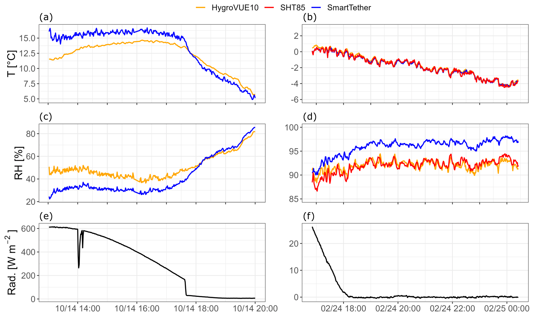
Figure 9Time series of (a, b) temperature (T) and (c, d) relative humidity (RH) for the SmartTether (blue line), SHT80 sensor (red line) and HygroVUE10 reference sensor (orange line) during two comparison experiments (left and right columns). Panels (e) and (f) indicate incoming shortwave radiation (Rad.) in black. Time is indicated in local time for both panels, (e) CEST and (f) AKST. The first comparison was performed in Brigerbad, Switzerland (46^∘18^′00^′′ N, 7^∘ 55^′16^′′ E), and the second was performed in Fairbanks, Alaska, USA (64^∘51^′12^′′ N, 147^∘51^′34^′′ W).

Download

Overall, the SmartTether provides reliable measurements when solar irradiance is low (overcast skies or at night) and/or wind speed is sufficiently high (> 1 m s⁻¹) to maintain the sensor horizontal. In other cases, measurements can be biased and data should be treated accordingly. To address this issue, a solution including two sensors (SHT85, Sensirion, Switzerland) in a shielding tube with active flow has been added to provide additional redundant T and RH measurements. Figure S1 shows the new radiation shield on the MoMuCAMS box.

4.1 Sampling strategies and MoMuCAMS performance validation

Three flight patterns have been utilized for sampling with MoMuCAMS. The flight pattern depends on the instrumental setup and the time resolution of the data acquisition. Fast profiles consist in a continuous ascent followed by a continuous descent and are performed to obtain a snapshot of the atmospheric column. Such a flight pattern is presented in a case study in Sect. 4.2.1. In this study, the velocity of the tether extension is 20 m min⁻¹. The ascent and descent rate of the Helikite depends on the line angle, but based on discussion in Sect. 2.2, it can vary between 13 and 20 m min⁻¹ for a zenith angle of 50 and 0^∘, respectively. The spatial resolution for instruments recording at 1 Hz is therefore between 0.2 and 0.3 m. In the configuration described in Sect. 3.3, the mSEMS has a vertical resolution between 13 and 20 m. For conditions with low particle number concentrations, the scan time might need to be increased to improve counting statistics, reducing even further its spatial resolution. Users will need to define the best combination of bin time and the number of bins (size resolution) to optimize the data quality and spatial resolution of the mSEMS.

Given the lower time resolution of the mSEMS compared to other instruments on board MoMuCAMS, a second flight strategy consists in a fast-ascending profile followed by a stepwise descent. Stops allow for the mSEMS to collect several scans at the given altitude. The length of the stop at a fixed altitude depends on the total scan time of the mSEMS (1 min per scan in this study) and should allow for the mSEMS to measure several scans to improve the counting statistic of the measured PNSD. Ultimately, the distance between each step and its respective duration varies according to the maximum altitude of the profile, desired time of flight, and atmospheric conditions such as temperature inversions or stratification. An example of such a flight pattern is presented in a case study in Sect. 4.2.2.

For airborne sampling for offline analysis, the Helikite is brought to a desired altitude (e.g., above the ABL or above a cloud, depending on the research question). Once the Helikite has reached the altitude, the filter samplers are activated remotely. For airborne sampling with the HFI, the number of stages used is usually reduced from six to three to optimize mass collection on filters, especially if sampling time is reduced because of flight duration restrictions imposed by regulations. The FILT typically samples for 1 h per channel. Section 4.2.3 shows results of two test flights for airborne sampling.

Altitude during flight is provided by the GPS of the SmartTether and is re-calculated during postprocessing of the data using the barometric formula of (Eq. 3)

where T₀ is the temperature at the surface; L₀= 6.5 K km⁻¹ is the mean environmental lapse rate; p₀ and p_b are the pressure at the surface and balloon height, respectively; R= 287 J kg⁻¹ K⁻¹ is the gas constant for dry air; and g is the Earth's gravitational acceleration. An uncertainty of ±1 m for the altitude was calculated using the root mean square error for a 3 h time series of altitude measurement at a known altitude.

4.2 Case studies

From 22 September to 14 October 2021, MoMuCAMS was deployed in a field campaign to study the vertical distribution of aerosols and trace gases in an Alpine valley in relation to the complex meteorological conditions of mountain regions. In addition to vertical profiling, ground-based measurements were performed to provide a continuous reference on the ground. A trailer with an inlet system was parked 30 m from the Helikite. Instruments from the MoMuCAMS system sampled from the trailer between flights. Additionally, a SEMS measured PNSD from 8 to 1100 nm, and a weather station (Campbell Scientific, USA) measured meteorological parameters on the ground.

The study site was located in Brigerbad, Switzerland (46.29^∘ N, 7.92^∘ E), in the Rhône Valley at an altitude of 653 m a.m.s.l. (above mean sea level). Typical weather patterns exhibited diurnal temperature cycles during the whole period. In response to the radiation and temperature diurnal cycle, katabatic winds typically blew from the east between 22:00 and 09:00 LT with a mean velocity of 0.9 m s⁻¹. For interpretation purposes, time is given in local time, corresponding to central European summer time (CEST or UTC+2). The wind typically transitioned to a cross-valley southerly wind around 10:00 LT and further developed into a stronger westerly valley wind in the afternoon. The diurnal cycle was also characterized by surface temperature inversions occurring frequently during clear-sky nights.

Several anthropogenic sources of atmospheric pollutants are located near the site, including industry, roads, private housing and agricultural fields.

In the following section, we present case studies with three different instrumental setups illustrating the various measurement capabilities of MoMuCAMS.

4.2.1 Case 1: evolution of aerosol and trace gas concentrations during a surface inversion dissipation

Six profiles (three ascents and three descents) were measured on a cloud-free day on 1 October 2021, from 08:50 to 12:30 LT. The instrumental setup for this flight included a combination of trace gas monitors (CO, CO₂ and O₃) and aerosol instruments to measure the total number concentration (aMCPC) and PNSD above 186 nm (POPS). The combination of trace gas and aerosol measurements can be used to identify atmospheric layers with different emission sources based on ratios between the different tracers.

Figure S11a shows the ground temperature (T), net radiation (NR) and wind speed (U) and direction evolution from 08:00 to 12:45 LT. At 09:30 LT, the sun rose from behind the mountains, which led to a sharp increase in NR, followed by a surface temperature increase. Winds at the surface remained low during the flights. Weak easterly katabatic winds were blowing until roughly 09:30 LT and then gradually developed into a cross-valley wind around 11:00 LT. Above 50 m, winds were slightly stronger (between 2 and 4.5 m s⁻¹), and their east-northeast orientation remained rather constant through the flights (Fig. 11b and c). Figure S11b and c show the ground-based measured PNSD and integrated total concentration (black dots), rising from 08:00 LT and peaking between 09:00 and 09:30 LT, followed by a gradual decrease until noon, which is consistent with the onset of convective mixing induced by surface warming. Figure 10d shows a time series of the balloon altitude. The color of each altitude point indicates the particle number concentration from 186 to 3370 nm (N_186−3370) measured by the POPS.

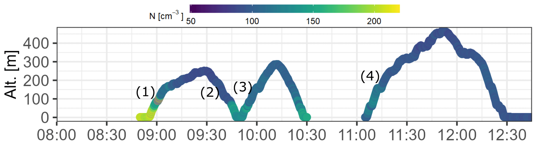
Figure 10Time series of balloon altitude above ground level (m) on 1 October 2022. The color scale indicates number particle concentration (186–3370 nm). Numbers in parentheses indicate the different profiles shown in Figs. 11 and 12. Location: 46^∘18^′00^′′ N, 7^∘55^′16^′′ E.

Download

Figures 11 and 12 show four different vertical profiles illustrating the evolution of the boundary layer. The selected profiles are indicated by numbers in parentheses in Fig. 10d. Colors indicate the starting time of each profile. Figure 11a shows a surface-based temperature inversion with a mean gradient of 1.8 ^∘C per 100 m⁻¹ during the first ascent starting at 08:55 LT (turquoise profile), indicative of a stable boundary layer (SBL) up to at least 250 m a.g.l. The top of the inversion cannot be determined as the maximum reached altitude was still within the inversion layer. Figure 12 shows vertical profiles of the particle number concentration and trace gas mixing ratios. The first profile shows a surface layer (SL) up to 50 m with increased yet rather homogenous concentrations compared to more elevated layers (> 150 m). N₇₋₁₈₆ and N_186−3370 concentrations were up to 7 and 2 times higher than concentrations measured above 150 m, respectively. Ground-based measurements indicate that surface particle number concentrations started increasing around 08:00 LT (Fig. 10b). The increase at the surface is explained by the morning rush hour and reduced mixing volume due to valley walls and stable atmosphere, as has been observed previously in similar valley locations (Chazette et al., 2005, or Harnisch et al., 2009).

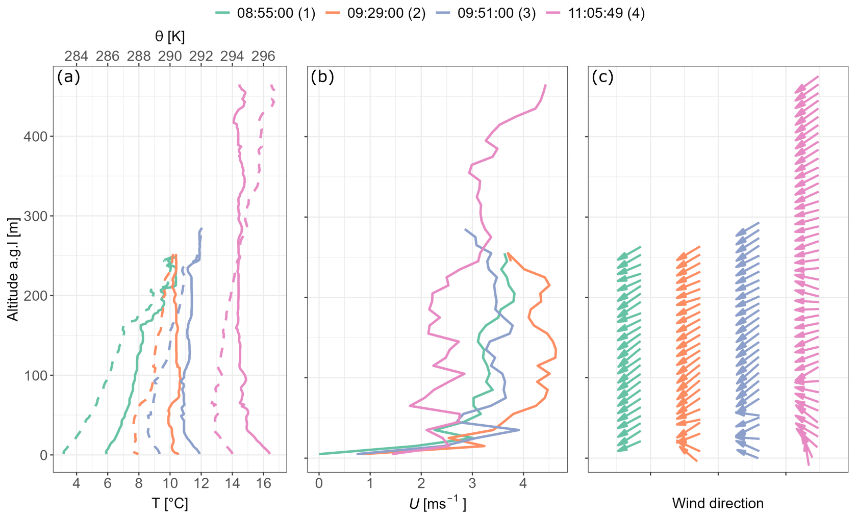
Figure 11Vertical profiles of (a) temperature (T – full lines) and potential temperature (θ – dashed lines), (b) wind speed (U) and (c) wind direction. Temperature is displayed at a 2 m spatial resolution, corresponding on average to 10 data points, whereas wind is displayed at a 10 m resolution, for an average of 25 data points.

Download

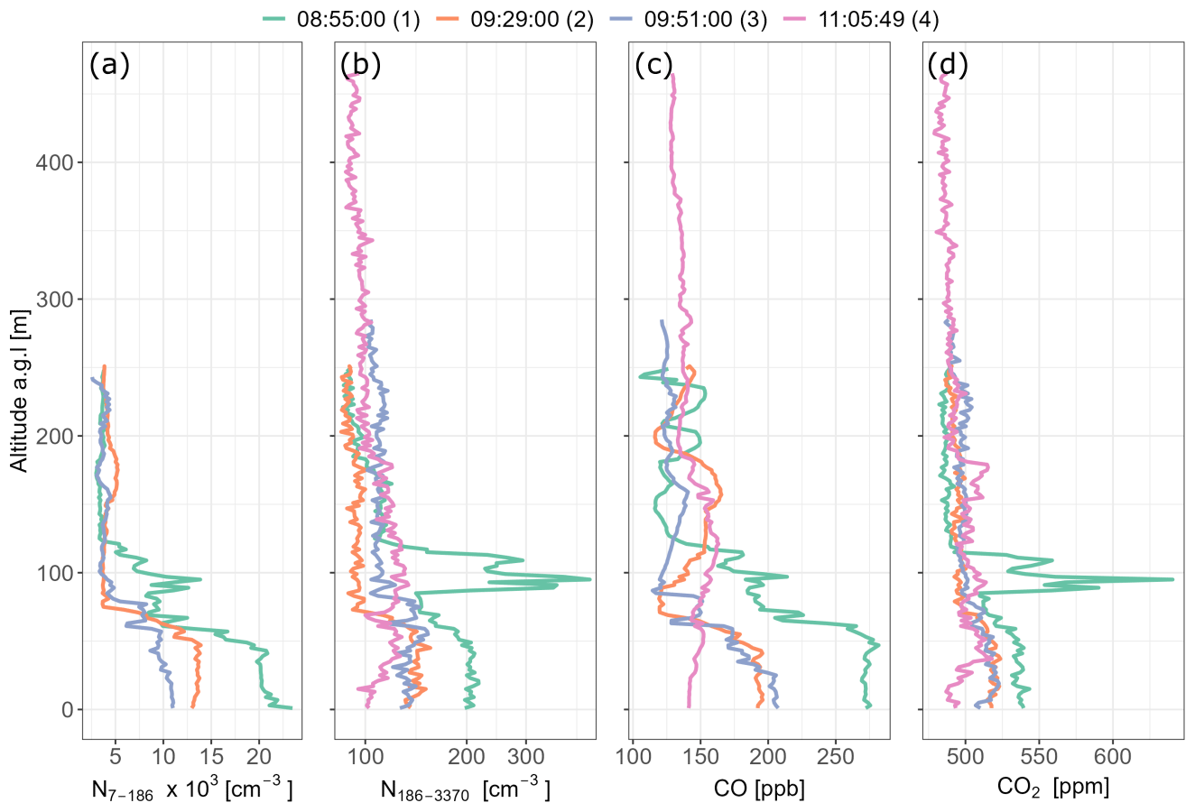
Figure 12Vertical profiles of the (a) particle number concentrations in the size range of 7 to 186 nm, (b) particle number concentration in the size range of 186 to 3370 nm, (c) CO mixing ratio and (d) CO₂ mixing ratio. Data are displayed at a 2 m spatial resolution, corresponding on average to 10 data points. The displayed time in panel (a) indicates the beginning of each profile.

Download

Between 80 and 125 m a.g.l., large peaks in the particle concentration and CO₂ mixing ratio were measured during the first ascent. These peaks were, however, not present on the following descent after 09:30 LT (Fig. 12, orange profile). At maximum peak intensity, the concentration of N₇₋₁₈₆ and N_186−3370 was about 3 and 4 times larger than above 150 m, respectively.

Compared to the SL, N₇₋₁₈₆ was 1.7 times lower at the plume altitude but N_186−3370 was 2 times larger. The CO₂ concentration shows an increase of 10 % at the peak compared to surface values. CO exhibits only a weak signal at the same altitude. The exact origin of the plume is not known. The increase in CO₂ mixing ratio might suggest that the particles were recently emitted from an anthropogenic source. The different gas and particle ratios between the SL and the plume layer suggest different source contributions to the two layers. Given the altitude of the plume and the stability of the atmosphere, it can be hypothesized that the source either was located at the same altitude or was located at the surface and had a higher injection height. The potential source could thus be either located on the valley slope or be a high stack from an industrial facility. It is not possible to say if the disappearance of the plume after the first flight was caused by the reduced atmospheric stability, which increased the dispersion and mixing of the plume, or by the termination of the emission process. This measurement however provides clear evidence that MoMuCAMS is effective in detecting plumes aloft and can be used to track emissions at higher elevations.

Not accounting for the above-discussed plume, concentrations in particles and gases decreased between 50 and 150 m (Fig. 12). This negative gradient can be explained by a progressive reduction in the mechanical turbulent mixing caused by wind shear at the surface.

Concentrations above 150 m show relatively homogenous profiles up to the maximum altitude with typically cleaner air. Given the atmosphere's stability during the first ascent, only a little or no vertical dispersion is occurring at these altitudes. Between the first ascent and the following descent, the surface temperature increased by 4.5 ^∘C in response to incoming solar radiation. The temperature of the entire column also increased, and the main surface-based temperature inversion dissipated (Fig. 11a). As the surface temperature increases between the first and last profile, convective mixing is induced and air from the residual layer is entrained into the surface layer. This phenomenon can be observed in Figs. 10c and 12, where the high concentration at the surface in the first profile, indicated by the yellow colors, gradually decreased for each profile. The surface dilution is observed for all tracers, and by 11:00 LT, all profiles appear rather homogenously distributed up to the maximum reached altitude. The efficient mixing effectively reduces particle and gas concentrations near the surface and alleviates air quality issues. The observed homogenous profiles suggest that the induced convective mixing and slope winds can transport polluted air from the surface to higher elevations, as previously reported by Furger et al. (2000) during the VOLTALP campaign in the Mesolcina Valley in southern Switzerland. Similar conclusions were drawn by Ketterer et al. (2014), who reported an increase in local boundary layer height and transport of aerosols from the valley bottom to the Jungfraujoch by slope winds.

4.2.2 Case 2: particle size distribution dynamics during the transition from a stable to a mixed boundary layer

Fourteen profiles (seven ascents and seven descents) were performed on a cloud-free day on 14 October 2021, from 06:50 to 12:30 LT. The instrumental setup for this flight included the mSEMS and the POPS to analyze the difference in PNSD at various elevations in the presence of a surface-based inversion and to investigate size-dependent aerosol mixing during the breakup of the inversion layer.

Figure S12 shows measurements at the surface and the altitude profile time series of the Helikite. The altitude profile (Fig. 13) shows an alternation of fast-ascending, descending, and stepwise profiles to allow for the mSEMS to collect more scans. Based on the integrated particle number concentration (N₈₋₂₈₀) of the mSEMS (not shown here) and N_186−3370 (Fig. 13, colored altitude profile dots) we distinguished a surface layer (SL) up to 70 m and a residual layer (RL) above 150 m. Similarly to the 1 October situation, a layer with a negative gradient of the particle number concentration is observed between 70 and 150 m. This layer is referred hereafter as the intermediate layer (IL).

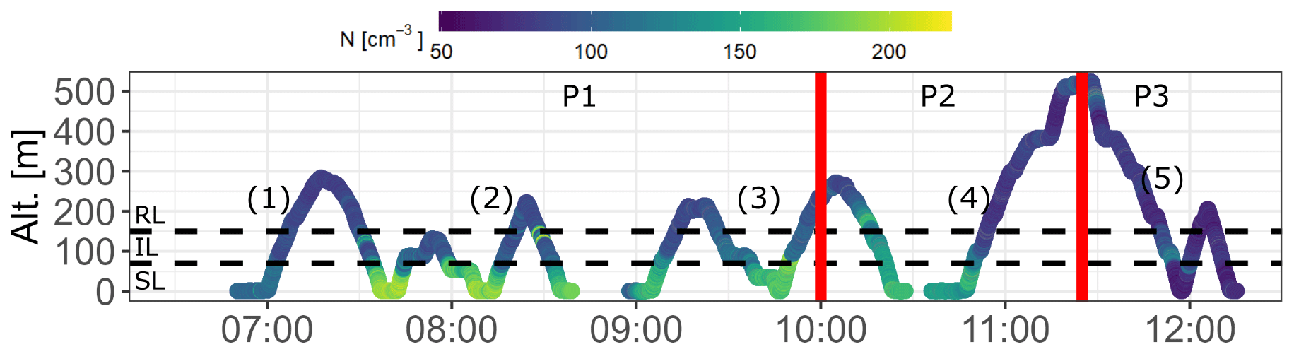
Figure 13Time series on 14 October 2022 of balloon altitude above ground level (m). The color scale indicates the particle number concentration (> 186 nm). Numbers in parentheses indicate the different profiles shown in Fig. 14. P1, P2 and P3 refer to the three time periods discussed in Fig. 15.

Download

A subset of collected temperature profiles, evenly spaced out and covering the whole flight period, has been selected to show the evolution of the atmospheric structure (Fig. 14). The numbered profiles are also indicated in Fig. 13 for more clarity.

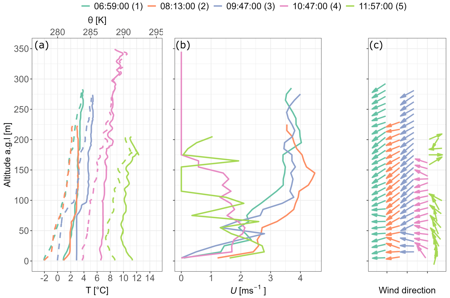
Figure 14Vertical profiles of (a) temperature (T – full lines) and potential temperature (θ – dashed lines), (b) wind speed (U) and (c) wind direction. Temperature is displayed at a 2 m spatial resolution, corresponding on average to 10 data points, whereas wind is displayed at a 10 m resolution, for an average of 25 data points.

Download

Figure 14a shows the warming of the atmosphere following sunrise and the erosion of a surface-based inversion.

Winds remained very low at the surface throughout the flights, with a slight dominance of the easterly direction until sunrise. Wind direction then changed due to warming of southerly exposed slopes (Fig. S12a). The vertical wind profile indicates increasing northeasterly winds with altitude during the first profiles. However, winds decreased after 10:45 LT and were almost inexistent during the last profiles, indicative of a transitioning regime between katabatic and valley winds. Figure 13 shows the evolution of the SL. Despite the presence of a temperature inversion that developed overnight, the concentration in the surface layer shows an evident increase after 07:15 LT (Fig. S12c) in response to increased traffic emissions. We then observe a dilution and a larger vertical extent of the SL after 10:00 LT. After 11:30 LT, the surface layer is not visible anymore.

Based on Fig. 13, three periods have been identified. The first period (P1) (07:30–09:59 LT) represents the accumulation of pollutants at the surface. From 10:00 to 11:15 LT (P2), we observe a slightly greater vertical extent of the concentrated layer, indicative of increased vertical mixing. Finally, after 11:15 LT (P3), the surface layer is eroded and the entire vertical column looks more homogenous. Note that although the total particle concentration shows a decreasing trend shortly after 10:00 LT, a peak of particles was measured around 10:40 LT. This sudden burst was probably related to a very close source of anthropogenic emissions from a truck or gardening activities on the nearby parking lot. These nearby emissions might have biased the surface concentrations of the ascending profile at 10:47 LT.

For each period, we investigated the PNSD measured with the Helikite to identify the main characteristics of each layer and see how they evolved with the development of the ABL. Results for PNSD between 8 and 500 nm are presented in Fig. 15. The distribution was obtained by merging data from the mSEMS and the POPS. The two datasets present an overlap between 186 and 280 nm. Left panels (a, c and e) show the color-coded evolution of the PNSD in each layer. The SL is represented on the lower panels for easier interpretation. Right panels (b, d and f) show the equivalent normalized distribution to better evaluate the relative contribution of different size modes to the PNSD. Normalization was done by dividing $\mathrm{d}N/\mathrm{d}\log D_{\mathrm{p}}$ values of each scan by the maximum $\mathrm{d}N/\mathrm{d}\log D_{\mathrm{p}}$ measured for the respective scan, yielding a maximum value of 1 for the main peak.

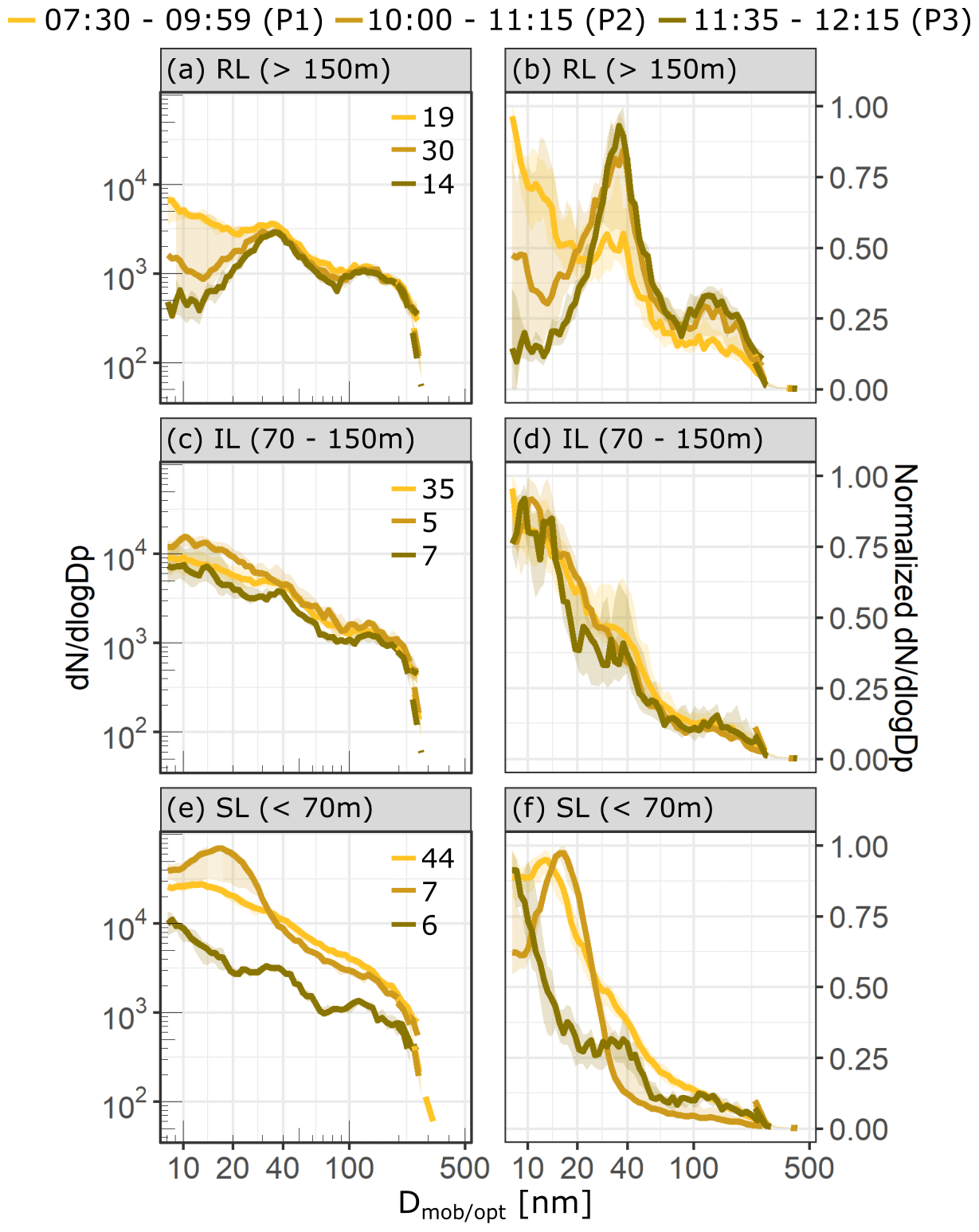
Figure 15Evolution of particle size distributions between 8 and 500 nm in the residual layers (> 150 m, a and b), intermediate layer (70–150 m, b and e) and surface layer (0–70 m, e and f). Solid lines indicate the median PNSD measured by the mSEMS, while shadings represent the interquartile range. Dashed lines represent the PNSD measured by the POPS. Colors indicate the three periods P1, P2 and P3. Panels (a), (c) and (e) represent the $\mathrm{d}N/\mathrm{d}\log D_{\mathrm{p}}$ size distribution. Numbers in the upper right corners indicate the number of scans collected per layer and period. Panels (b), (d) and (f) show normalized distributions, where each $\mathrm{d}N/\mathrm{d}\log D_{\mathrm{p}}$ value of a scan was divided by the maximum $\mathrm{d}N/\mathrm{d}\log D_{\mathrm{p}}$ measured for the respective scan.

Download

The SL (Fig. 15e and f) is characterized by the highest concentration during P1 (yellow) and P2 (light brown). Looking at the normalized distribution, the SL seems dominated by a small Aitken mode around 15 nm. A second mode is also visible during P1 between 30 and 40 nm (small shoulder in the distribution). This second mode is also present in the upper layers and represents most likely aged particles emitted during the previous days. At P2, this larger Aitken mode is not visible anymore because of the stronger dominance of freshly emitted particles at the surface. Note the main peak at P2 (Fig. 15f) has shifted to the right compared to P1, indicative of potential growth of freshly emitted particles. Looking at the RL (Fig. 15a and b), the PNSD exhibits a bimodal distribution with a main larger Aitken mode at 40 nm and an accumulation mode at roughly 150 nm. This distribution seems to represent the background boundary layer composition of particles emitted from previous days (Aitken mode) and older particles that either remained suspended in the ABL for longer or were entrained from the free troposphere. At P1, the PNSD also shows contributions from smaller nucleation mode particles. It can be hypothesized that emissions from cars and residential heating on the valley sides could directly contribute to this increase of smaller particles in the RL. The size distribution is, therefore, the result of the mixing between the aged mode from the previous day and fresh emissions from higher up in the valley. At P2, the contribution of the nucleation mode is lower but with large variability, indicative of a transition to lower car traffic on the valley sides. A more systematic analysis under similar conditions would need to be performed to see if this phenomenon regularly occurs and better understand the underlying processes.

The IL shows a similar feature to both the SL and RL. At P1, the PNSD shows more similarity with the RL but with a less pronounced Aitken mode peak (Fig. 15c and d). At P2, the influence from the surface becomes clearer as the overall concentration of nucleation and Aitken mode particles increases similarly to the SL. This indicates the onset of boundary layer growth and upward transport of surface emissions. At P3 (dark brown), the IL and SL show very similar characteristics with the same concentration magnitudes for a nucleation mode peak, the larger Aitken mode (40 nm) and the accumulation mode with overall lower total concentration indicative of a larger mixing volume due to increased ABL height. The observed increase in the nucleation mode contribution could be explained by a combination of new particle formation (NPF) without growth and direct emissions of ultrafine particles by cars. However, due to a limited number of measurements in the layer, the actual source of the nucleation mode contribution remains uncertain. The RL shows similar features and concentration magnitudes as the lower layers for the Aitken and accumulation mode, but not for the nucleation mode, potentially indicating that these particles were only emitted later and did not have time to be transported higher up yet and where thus not captured. The bimodal distribution observed in the former RL at P3 seems to constitute the background size distribution of the mixed boundary layer (ML) in the valley.

Overall, in the presence of a stable boundary layer, surface pollution is tightly linked to traffic emissions and is constrained in a shallow layer about 70 m thick. This can lead to a rapid accumulation of pollutants. Ultrafine particles around 15 nm dominate the number concentration, which can be up to 5 times higher than the concentration of a mixed-boundary layer if we refer to the previous case study (Sect. 4.1). Particles that are not lost via coagulation or dry deposition remain in the boundary layer after the development of a ML and grow to a size of about 40 nm. These particles then constitute the boundary layer's particle background along with particles in the accumulation mode. The development of the ML in response to surface heating is fast, and the concentrated surface layer is typically diluted within 1 to 2 h.

4.2.3 Examples of offline chemical analysis of airborne samples

Two test flights of airborne sample collection were performed on 28 September and 7 October 2021. For both flights, MoMuCAMS was equipped with the HFI for aerosol chemical analysis, the eight-channel filter sampler (FILT) for SEM and TEM analysis, and the POPS. The flight pattern for both flights was similar. After reaching a desired sampling altitude, the HFI pump was turned on remotely while the balloon hovered at the same altitude. Simultaneously, the FILT sampled for roughly 1 h per channel. As described in Sect. 4.1, the aim of airborne filter sampling is to reach layers decoupled from the surface. However, given the vertical extent of the daytime mixed ABL during the field campaign and the tether length, sampling was performed in the mixed ABL and constituted mainly a proof of concept of the sampling system. In both cases, the measured vertical profiles during ascent and descent indicated a well-mixed atmosphere with similar N_186−3370 concentrations throughout the entire column. The temperature profiles indicated an adiabatic lapse rate. An estimation of the aerosol mass concentration during sampling time was calculated from PNSD measurements from the POPS. The PNSD was converted to a volume size distribution and integrated over all size bins to obtain the total volume concentration. The volume concentration was then converted to a mass concentration, assuming a mean particle density of 1.6 g cm⁻³, given the predominance of anthropogenic sources (Pitz et al., 2003). Flights 1 and 2 had average concentrations of 3.58 (1.43) and 1.48 (1.37) µg m⁻³, respectively. The values in parentheses indicate the standard deviation of the measured mass concentration. Due to increased wind conditions (from 1.5 (2) to 9 (5) m s⁻¹ for flight 1 (2)) between the beginning and end of sampling, the altitude of the balloon decreased slightly. Table 4 provides details of both flights. Additionally, samples were also collected at the surface before flight 1 and before and after flight 2 to obtain a ground reference. Collected aerosols have been analyzed for element concentrations (see Sect. S7), and results for Cu and Se are presented here as an example.

Table 4Summary of ground and flight filter sampling.

Download Print Version | Download XLSX

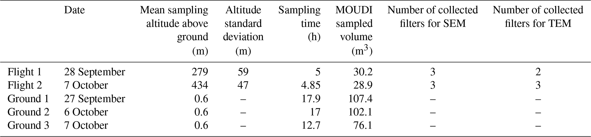
Figure 16 shows results of samples collected on the ground (a and c) and during flight (b and d). Ground sampling was performed with six stages and an after filter collecting all remaining particles below the lowest cutoff, while flights were performed with three stages only (0.44, 1 and 2.5 µm). Due to the low detection limit for Se, Se could be detected in almost all filters collected on the ground (between 12 to 18 h sampling time) and during flight (over 5 h). Due to higher Cu background in filters and thus a higher detection limit, Cu could mainly be detected in filters collected at the ground. Only one Cu measurement in the 1–1.4 µm range was above the detection limit for the aerosols collected during flight. The main limiting factor is the small aerosol mass concentrations obtained for the flight samples, which resulted in this case from a rather short sampling time. Great care must thus be taken in future studies in terms of sampling strategy to ensure that the amount of collected material is sufficient for chemical analysis, especially in polar regions where mass concentration is typically much lower.

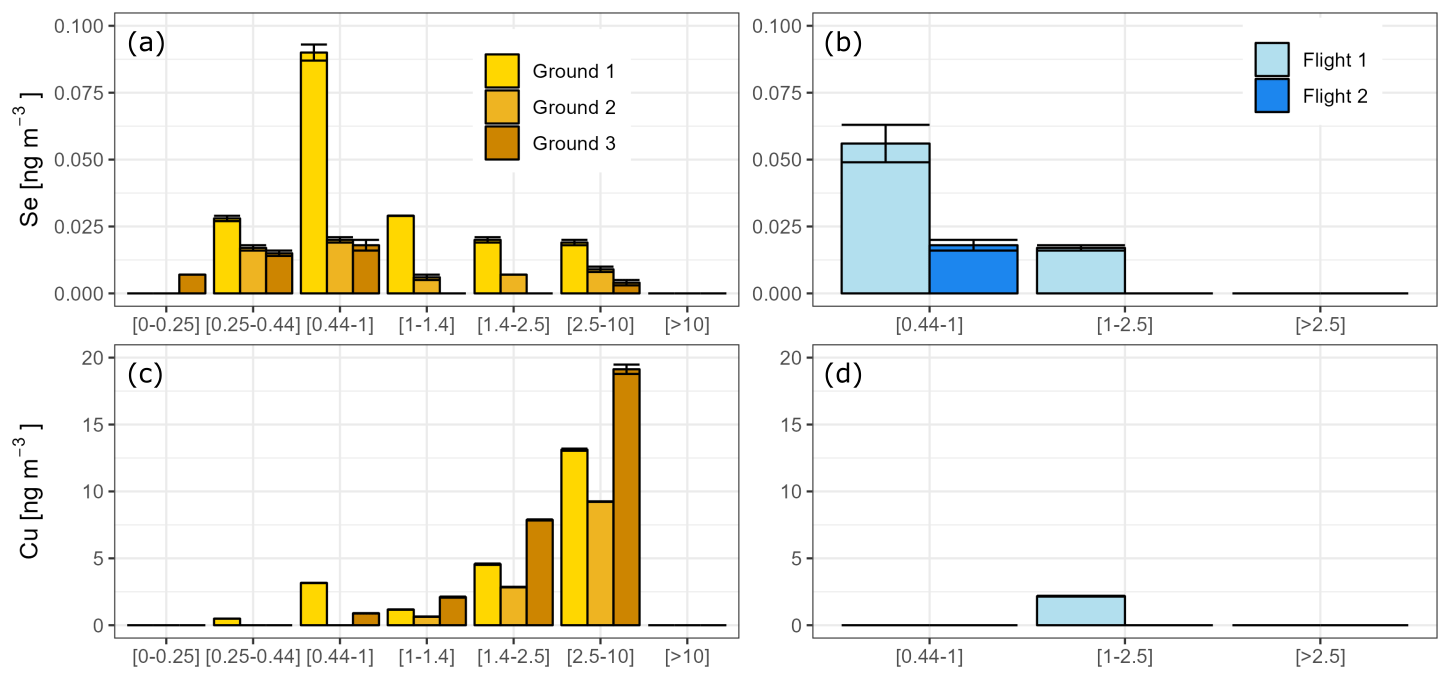
Figure 16Size-segregated measured concentrations by ICP-MS/MS (a–b) of selenium (Se) (a) at the surface and (b) during flight and (c–d) of copper (Cu) (c) at the surface and (d) during flight. The absence of a colored bar indicates that measured values were below the detection limit.

Download