the Creative Commons Attribution 4.0 License.
the Creative Commons Attribution 4.0 License.
 | 20 Dec 2023
An open-path observatory for greenhouse gases based on near-infrared Fourier transform spectroscopy
Tobias D. Schmitt
Jonas Kuhn
Ralph Kleinschek
Benedikt A. Löw
Stefan Schmitt
William Cranton
Martina Schmidt
Sanam N. Vardag
Frank Hase
David W. T. Griffith
Monitoring the atmospheric concentrations of the greenhouse gases (GHG) carbon dioxide (CO2) and methane (CH4) is a key ingredient for fostering our understanding of the mechanisms behind the sources and sinks of these gases and for verifying and quantitatively attributing their anthropogenic emissions. Here, we present the instrumental setup and performance evaluation of an open-path GHG observatory in the city of Heidelberg, Germany. The observatory measures path-averaged concentrations of CO2 and CH4 along a 1.55 km path in the urban boundary layer above the city. We combine these open-path data with local in situ measurements to evaluate the representativeness of these observation types on the kilometer scale. This representativeness is necessary to accurately quantify emissions, since atmospheric models tasked with this job typically operate on kilometer-scale horizontal grids.
For the operational period between 8 February and 11 July 2023, we find a precision of 2.7 ppm (0.58 %) and 18 ppb (0.89 %) for the dry-air mole fractions of CO2 (xCO2) and CH4 (xCH4) in 5 min measurements, respectively. After bias correction, the open-path measurements show excellent agreement with the local in situ data under atmospheric background conditions. Both datasets show clear signals of traffic CO2 emissions in the diurnal xCO2 cycle. However, there are particular situations, such as under southeasterly wind conditions, in which the in situ and open-path data reveal distinct differences up to 20 ppm in xCO2, most likely related to their different sensitivity to local emission and transport patterns.
Our setup is based on a Bruker IFS 125HR Fourier transform spectrometer, which offers a spacious and modular design providing ample opportunities for future refinements of the technique with respect to finer spectral resolution and wider spectral coverage to provide information on gases such as carbon monoxide and nitrogen dioxide.
- Article
(7103 KB) - Full-text XML
- BibTeX
- EndNote


Current climate change is driven by anthropogenic emissions of carbon dioxide (CO2) and methane (CH4). The international community has pledged itself to limiting global warming to below 2 ∘C and ideally below 1.5 ∘C compared to the preindustrial era (United Nations Framework Convention on Climate Change, 2015). Thus, substantial reductions of CO2 and CH4 emissions will be required in the coming years. Urban areas are major contributors to anthropogenic greenhouse gas (GHG) emissions (e.g., Marcotullio et al., 2013) and their reporting entails considerable uncertainties (Gurney et al., 2021). Monitoring of these emissions through atmospheric concentration measurements provides a tool to verify reported emission rates and to improve on the precision and spatiotemporal granularity of emission inventories (e.g., Mueller et al., 2021). This, in turn, might help effective implementation of emission reduction measures.
Atmospheric CO2 and CH4 concentrations above localized source regions can be measured by spectrometers on satellites (e.g., Nassar et al., 2017; Kiel et al., 2021), by ground-based sun-viewing spectrometers (e.g., Wunch et al., 2011; Frey et al., 2019), and by in situ sensors deployed in networks or on moving platforms (e.g., Shusterman et al., 2016; Fiehn et al., 2020). Recently, techniques have emerged that measure the GHG concentrations integrated along long horizontal absorption paths above urban areas (e.g., Dobler et al., 2013; Waxman et al., 2017; Griffith et al., 2018). This configuration has the particular advantage that the observed path-integrated gas concentrations are (1) more sensitive to emission patterns than vertical column-average concentrations accessible through satellites and ground-based sun-viewing techniques and (2) more representative than in situ data for typical grid scales of atmospheric transport models that are used to translate the observed concentration gradients into emission rates. The latter advantage might be particularly important for urban regions with spatially highly structured source patterns.
Various absorption spectroscopic techniques have been suggested for long open-path measurements of CO2 and CH4. There are systems that utilize continuous wave lasers at a few discrete spectral points (Dobler et al., 2013; Lian et al., 2019). Typically one spectral point is located on a strong absorption feature of the target gas and another one in the transparent region right next to it. This approach does not provide any information on the shape of the target absorption feature. Tunable diode lasers (TDLs) extend this technique to measurements of a full absorption line, with the potential to measure a few spectrally close absorption lines (Bailey et al., 2017). Laser frequency combs, e.g., operated in a dual-comb spectroscopy setup (Coddington et al., 2016), can improve on this by covering a few hundred wavenumbers and measuring full rotational–vibrational absorption bands with dozens of lines (Truong et al., 2016; Waxman et al., 2019). This can provide access to temperature information within the spectrum. Fourier transform spectroscopy (FTS) can measure across spectral intervals of several thousand wavenumbers simultaneously, giving access to a plethora of species at the same time. FTS open-path systems working in the mid-infrared (MIR) are well established (Wiacek et al., 2018; Bai et al., 2020; You et al., 2021). MIR FTS systems are typically limited by low brightness of the light source, resulting in maximum atmospheric absorption paths lengths of a few hundred meters. Near-infrared (NIR) FTS systems can make use of hotter thermal light sources like halogen lamps and with that achieve path lengths exceeding kilometers.
Such NIR FTS open-path measurements for CO2 and CH4 were pioneered by Griffith et al. (2018) in a demonstration study for the city of Heidelberg, Germany. Their system was built around an IRCube FTS manufactured by Bruker Optics – a compact, robust spectrometer. Since then, their setup has been improved and developed into a portable version suitable for field deployments (Deutscher et al., 2021). We followed a complementary path and built a new open-path system in Heidelberg with the goal of designing a permanent atmospheric observatory suitable for future methodological explorations and for long-term measurements of CO2 and CH4 above Heidelberg. To this end, we used a Bruker Optics IFS 125HR FTS that, due to its modular and spacious layout, allows for configuring the spectral resolution and for deploying various detectors giving access to various spectral ranges.
Here, we report on the initial setup of the observatory and its performance for measuring CO2 and CH4 concentrations along a 1.55 km path above Heidelberg, essentially mimicking the overall configuration of the demonstrator study by Griffith et al. (2018) but demonstrating the performance of the IFS 125HR FTS. Section 2 elaborates on the experiment and the methods used, with a particular focus on how the 125HR FTS is used in the long open-path setup. Section 3 reports on the performance for months-long CO2 and CH4 observations and discusses the observations in comparison to the local in situ records. Section 4 concludes the study with a discussion of future exploration possibilities.
2.1 Deployment configuration
The location of the measurement path above the city of Heidelberg is shown in Fig. 1, which is the same as in Griffith et al. (2018). All active components (spectrometer, light source) are located at the west end of the path in the rooftop observatory (Fig. 2, left) of the Institute of Environmental Physics (IUP). A reflector array is located at the east end of the path on the roof of the old physics institute (OPI) (Fig. 2, right). The length of the path is 1553±1 m as determined with a laser rangefinder. The open-path instrument is situated 33 m above ground. The ground below is mostly flat (within 5 m) and rises nearly linear in the last 200 m by about 20 m. The typical roof height of the residential area below the absorption path is around 15 m. The air inlet for the in situ analyzer, which is used for comparison, is located at the western end on the roof of the IUP. The in situ analyzer is a cavity ring-down spectroscopy (CRDS) system (G2201-i, Picarro, Inc., Santa Clara, CA). The whole system, including the drying and calibration setup, is described in detail by Hoheisel et al. (2019) and Hoheisel (2021). Measurements of temperature, wind speed, wind direction, humidity, and pressure are regularly taken by a weather station located on the roof of the IUP.
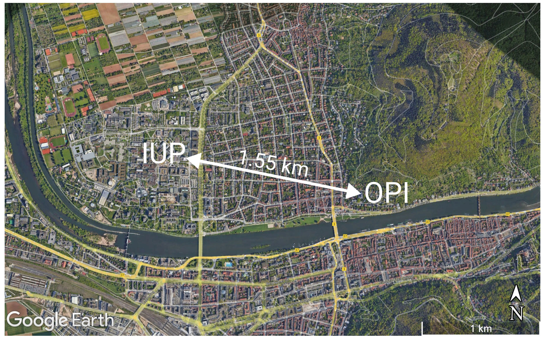
Figure 1Aerial view of the measurement path above the city of Heidelberg, Germany. All active components are located at the western end of the path at the Institute of Environmental Physics (IUP). The reflector array is located on the roof of the old physics institute (OPI). The light path passes predominantly over a residential area. At the western end (just 120 m east of the IUP) the path crosses a major road with heavy commuter traffic. Base map: © Google Earth.
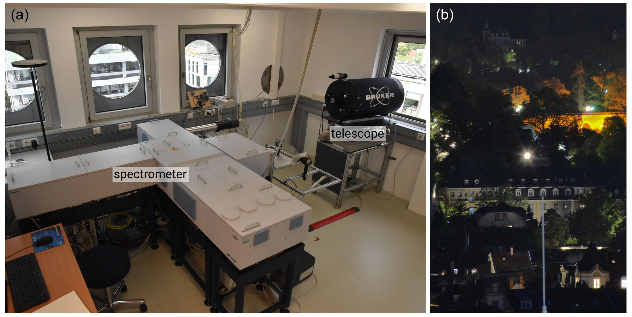
Figure 2(a) Overview of the rooftop observatory of the IUP with the IFS 125HR spectrometer in the center, as well as the telescope pointing out a window. (b) View along the light path at night, with the reflector array on top of the OPI shining bright in the center of the picture.
The setup in the current hardware configuration has been operating since 8 February 2023 and the measurements discussed here extend until 11 July 2023. During this time, the instrument was operated in different configurations concerning the integration time as well as spectral resolution. Further, the measurements were interrupted on several occasions, when the FTIR instrument was needed for other experiments.
2.2 FTIR setup and open-path optics
Figure 3 shows a sketch of the optical setup. The internal light source of the spectrometer (a 20 W halogen lamp) is collimated and transmitted through the interferometer of the IFS 125HR (focal length of collimator: 418 mm, field stop: 2 mm). The modulated beam of light is coupled into a bundle of fibers (6 × 200 µm, length 5 m, VIS–IR silica), which we call the transmitting fibers. At the other end, the transmitting fibers are grouped around a single central fiber and are positioned close to the focus of the telescope mirror (focal length: 813 mm, diameter: 406 mm). The telescope mirror collimates the modulated light of the transmitting fibers and sends it through the atmosphere to an array of retro-reflectors (the array consists of 41 solid UV quartz cube corners, each with a diameter of 53 mm). The retro-reflector array returns the beam of light back to the telescope, where it is coupled into the single central fiber (200 µm, length 5 m). At the other end of this receiving fiber the light is focused on the photodiode of an external detector of the spectrometer. This type of open-path telescope design and fiber system were originally developed for differential optical absorption spectroscopy (DOAS) measurements. An extensive description of the system and an in-depth analysis of the optical throughput is provided in Merten et al. (2011).
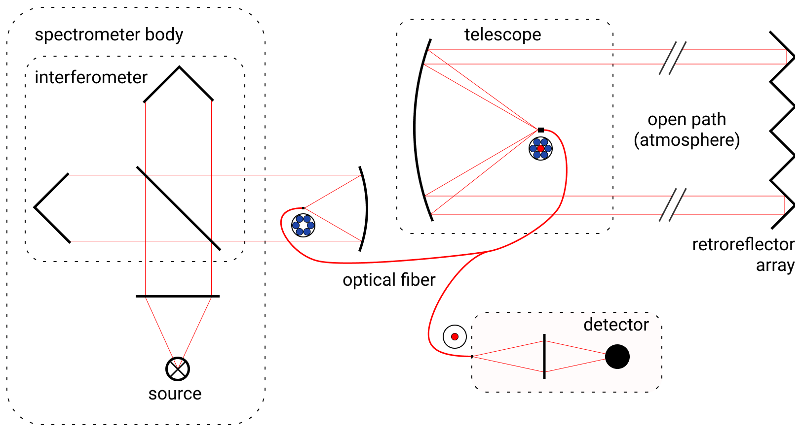
Figure 3Schematic drawing of the optical setup. The light source is modulated in the interferometer of the spectrometer and coupled into a bundle of six fibers (blue). These six fibers transport the light to a telescope, where it is collimated and sent along the open path on an array of retro-reflectors. The reflectors return the beam of light to the telescope where it is collected by a single central receiving fiber (red). From this fiber the light is focused on a detector.
For the target gases CO2 and CH4 relevant here, the detector is an InGaAs diode with a lower-frequency cut-off around 4200 cm−1. The quartz cube corners also cut off at around 4200 cm−1. To high frequencies, the spectrum is limited by a filter at around 9200 cm−1. The current setup is also equipped with Si and GaP detectors for the UV–visible spectral range, but these were not used here.
Compared to Griffith et al. (2018), the new setup modulates the light in the interferometer before sending; i.e., it is the interferogram (instead of the lamp spectrum) that travels along the absorption path. This has the advantage that scattered sunlight does not disturb the spectrum, and thus background measurements (with the lamp blocked) are not required. Any light that is collected in the telescope but not modulated by the interferometer contributes to the total photon flux on the detector, only increasing shot noise but not confounding the spectral information.
The FTS instrument itself was operated in three different configurations throughout the reported time frame. Our default mode of operation was chosen to be similar to Griffith et al. (2018) to allow for easy comparison. In this mode, we average 34 interferograms over a time span of approximately 5 min. The interferograms are measured double-sided using a maximum optical path difference (OPDmax) of 1.8 cm, which corresponds to a nominal resolution of about 0.55 cm−1. The scanner operates with 10 kHz scanning speed at the reference He–Ne laser line. The Fourier transform is performed using the standard Merz phase correction and a Norton–Beer medium apodization function. These settings were employed from 8 February until 22 March and from 25 May until 11 July. A typical spectrum recorded with these settings is shown in Fig. 4.
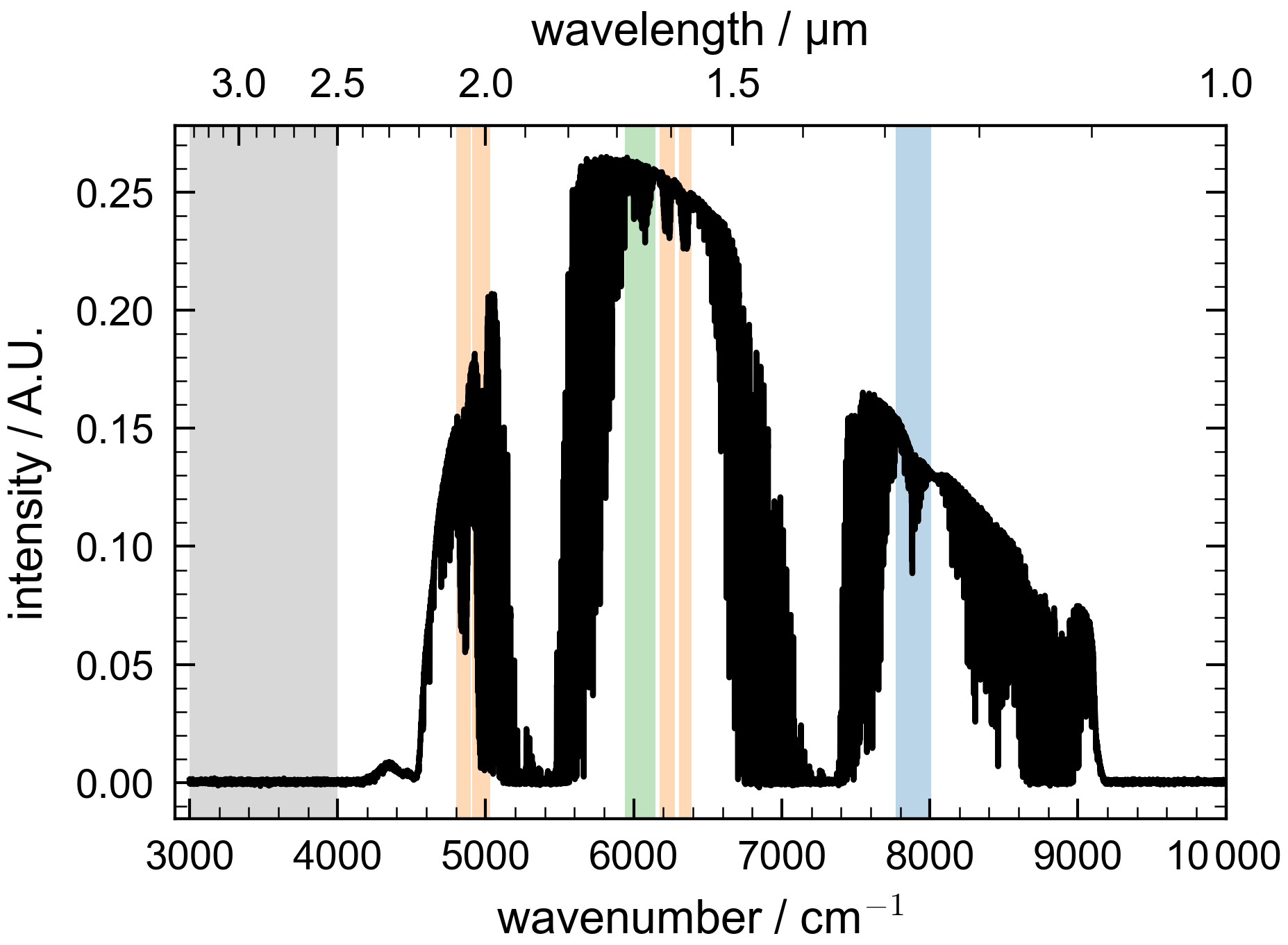
Figure 4Typical spectrum measured over 5 min with a resolution of 0.55 cm−1 and an SNR of 600. Target windows are highlighted in color: O2 (blue), CO2 (orange), CH4 (green). The off-band window, where we gather noise information, is marked in grey.
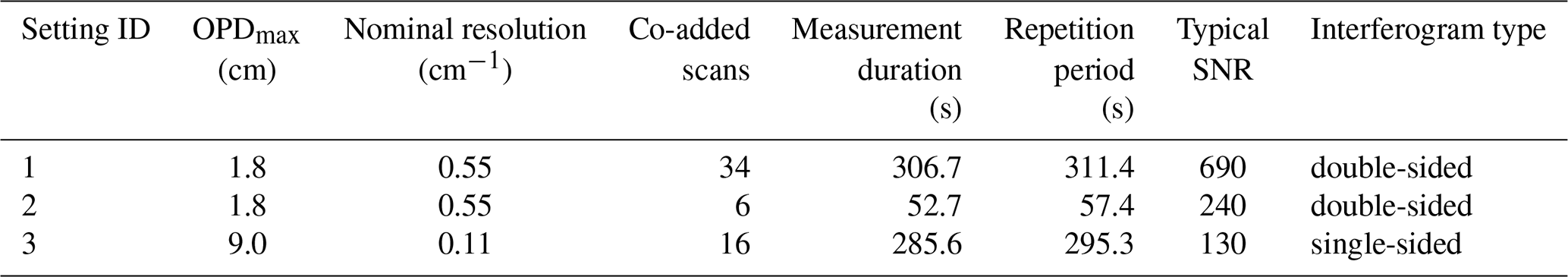
Apart from these default settings, we experimented with shorter averaging times of approximately 1 min from 23 March until 10 May, as well as with higher resolutions of approximately 0.11 cm−1 (OPDmax = 9 cm) from 11 until 24 May. Table 1 lists the details of the utilized instrument settings and the resulting times. All measurements are resampled to a regular 5 min grid to combine the different modes of operation.
The signal-to-noise ratio (SNR) was determined by taking noise information from the white noise in the off-band and using the spectral intensity at around 6300 cm−1 as a measurement for signal to allow for comparison with Griffith et al. (2018). The SNR was typically between 500 and 700 for the default mode of operation.
2.3 Spectral analysis and trace gas retrieval
We retrieve the path-integrated column densities (CDs) of the target gases from the measured spectra with a spectral fit. The forward model simulates the spectra based on the following input parameters: assumed gas column density (CD), spectral absorption cross-sections, temperature, and pressure. It further takes into account the instrument line shape (ILS) of the FTS, a spectral shift, and a polynomial to represent the continuum. The radiative transfer in the forward model is limited to a simple implementation of the Beer–Lambert law. The forward model and retrieval are implemented in Python.
The absorption cross-sections are calculated using the Voigt implementation of the HITRAN interface HAPI (Kochanov et al., 2016). We use line-by-line data provided in the HITRAN2020 database (Gordon et al., 2022). For the CO2 bands at 5000 cm−1, we use additional line-mixing corrections (Hartmann et al., 2009; Lamouroux et al., 2010). In the O2 band at 7900 cm−1, we account for collision-induced absorption (CIA) by fitting a pseudo-absorber. The absorption cross-sections for this pseudo-absorber are calculated using a temperature- and pressure-dependent air mass (via the ideal gas law) and the CIA data currently provided by HITRAN for O2–air interaction (Karman et al., 2019).
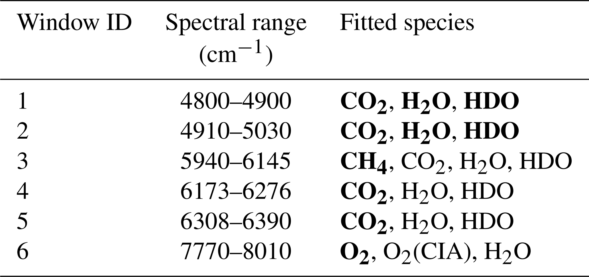
For fitting, the spectra are cut into various spectral windows, which contain the spectral signal of several target gases. Table 2 lists the windows used here, their spectral range, and all fitted species. All species are assumed with the HITRAN2020 standard mixture of isotopologues, except for H2O and HDO, which we fit separately.
Table 2Spectral windows and corresponding fitted trace gases. The main absorbers are highlighted in bold for each window.
The retrieval uses a Levenberg–Marquardt implementation for least-squares optimization. The differences between forward simulated spectra and the measurements are weighted by a noise estimation taken from the off-band (3000–4000 cm−1). We optimize the trace gas CD for each species. If gases need to be considered for several spectral windows, we fit their CDs separately per window and a posteriori calculate an average CD weighted by the propagated noise error. Temperature is fitted, while pressure is kept fixed at the measurement of our weather station. A spectral shift, as well as a background polynomial of degree 2, is also fitted in each window. In window 6, this polynomial is of degree 5 due to the width of the window.
The ILS of the instrument is described by a fixed set of parameters according to the simple model described in Hase et al. (1999). The parameters are the field of view (FOV) of the instrument and a single parameter for modulation efficiency and phase error each. We estimate modulation efficiency and phase error using 200 consecutive measurements taken on 26 February 2023. For each measurement a retrieval is performed as described above, but with ILS modulation efficiency and phase error as additional free parameters. The mean of these results for modulation efficiency and phase error is taken to simulate the ILS. The FOV is calculated to 4.78 mrad from geometrical parameters of the instrument.
2.4 Dry-air mole fractions
For comparison to external CO2 and CH4 data, e.g., provided by in situ measurements or by models, it is convenient to translate the path-average CDs into path-average dry-air mole fractions (e.g., in units ppm). In the scope of this study we calculate dry-air mole fractions xdry by ratioing the measured CD of the target gas CDtarget with the measured CD of O2 and multiplying with the O2 dry-air mole fraction.
It is also possible to forgo the measured O2 CD and calculate the dry-air mass from information on temperature, pressure, humidity, and pathlength. Since these values can be measured quite precisely, the results are typically up to an order of magnitude more precise than the measured O2 CD, so the precision of dry-air mole fractions should only be dominated by the precision of the target gas CDs. Because of this, Griffith et al. (2018) employed this method.
To compare the two methods, we calculated CDs of dry-air CDdry as follows: for temperature we use the retrieved path-averaged temperature T (as described in Sect. 2.3), for pressure the meteorological pressure p from the weather station at the institute, and for pathlength l as measured with a laser rangefinder. As a measure of humidity, we decided to directly take the measured CD of H2O vapor and subtract it from the calculated wet-air CD. This leaves us with the following equations (with kB being the Boltzmann constant).
2.5 Precision of time series
To estimate the precision of measured quantities (like target gas CDtarget, dry mole fractions xdry, or temperature), we took an empirical approach: we calculated the standard deviation among all differences between two consecutive measurements. By dividing the standard deviation by , we get the standard deviation for a single measurement. This is our measure for the mean precision of time series of measured quantities.
2.6 Bias correction to in situ data
The spectroscopically inferred open-path dry mole fractions require bias correction to ensure compatibility with other data sources such as in situ concentration measurements. This is necessary since the spectroscopic parameters, such as line strengths and broadening coefficients, tabulated in HITRAN feeding into the calculation of absorption cross-sections typically show inconsistencies between absorption bands, and their calibration has errors (e.g., Birk et al., 2021). This can easily lead to offsets on the percent scale for spectroscopic remote sensing measurements (e.g., Malarich et al., 2023). In situ instruments are calibrated to known standard gas mixtures and hence they are highly accurate (Hall et al., 2021). We operate such in situ measurements at the IUP, and hence we can bias-correct our open-path data with the in situ data. However, in situ and open-path instruments, by nature and intention, measure different bodies of air. Thus, the bias correction should be performed under atmospheric conditions when the local mole fractions at IUP are representative of the path-averaged mole fractions across the city, i.e., when there is no relevant effect from local emissions compared to the bulk concentration in the boundary layer. To select such conditions, we examine the histograms of xCO2 and xCH4 measured by the two instruments. Figure 5 shows that theses histograms have a peak at low mole fractions and a long tail toward high mole fractions. Since our sampling area and period are dominated by emissions rather than uptake for both species the tail corresponds to episodes wherein local emissions influence the concentration measurements significantly, and thus horizontal gradients are likely. The peak at lower concentrations corresponds to background conditions for which local emissions are less important, and thus we expect smaller gradients. To derive a correction factor, we visually identify these peaks and select the background measurements by filtering for observations which are coincident in both peaks. The correction factor is the mean of the ratio between the open-path and in situ data for all these background measurements. It amounts to approximately 0.9784 for xCO2 and 0.9887 for xCH4. We performed this analysis once with a subset of the data of about 6 weeks, roughly in the middle of the time series, to remove the general offset. From sensitivity studies, wherein we performed this bias correction with different subsets of the data, we estimate the accuracy of this method to about 1 ppm for xCO2 and 10 ppb for xCH4. In these sensitivity studies we cannot observe a trend or drift within in the full dataset. Hence, we decided to perform a single correction of the global offset. These factors are applied to all discussed open-path mole fractions from here on.
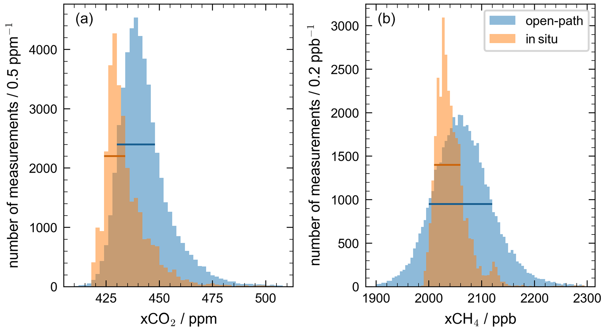
Figure 5Histogram of measured dry-air mole fractions for xCO2 (a) and xCH4 (b) from the in situ and open-path instrument. The expected peak of low concentration when measuring background air is clearly visible for both instruments. For xCO2 (xCH4), there are 33 426 (37 633) measurements in the selected peak area (blue and orange bar, respectively) for the open-path instrument and 17 064 (22 127) measurements for the in situ analyzer. A total of 13 633 (16 525) of those are coincident in time. Calculating correction factors for all these measurements and taking the mean yields a correction factor of 0.9784 (0.9887).
3.1 Quality of spectra and fit
Residuals of the spectral fit are illustrated in Fig. 6 for the spectral windows (see Table 2). Spectral residuals of individual 5 min measurements are typical below 1 % of the spectral intensity and mostly dominated by noise, while averaging over longer timescales reveals systematic patterns. In windows 1 and 2, the systematic effects are of the same order of magnitude as the noise. Statistical evaluation of the noise for the different absorption windows shows Gaussian noise. The noise also matches the noise estimation in scale from the off-band, after subtracting the average systematic effects.
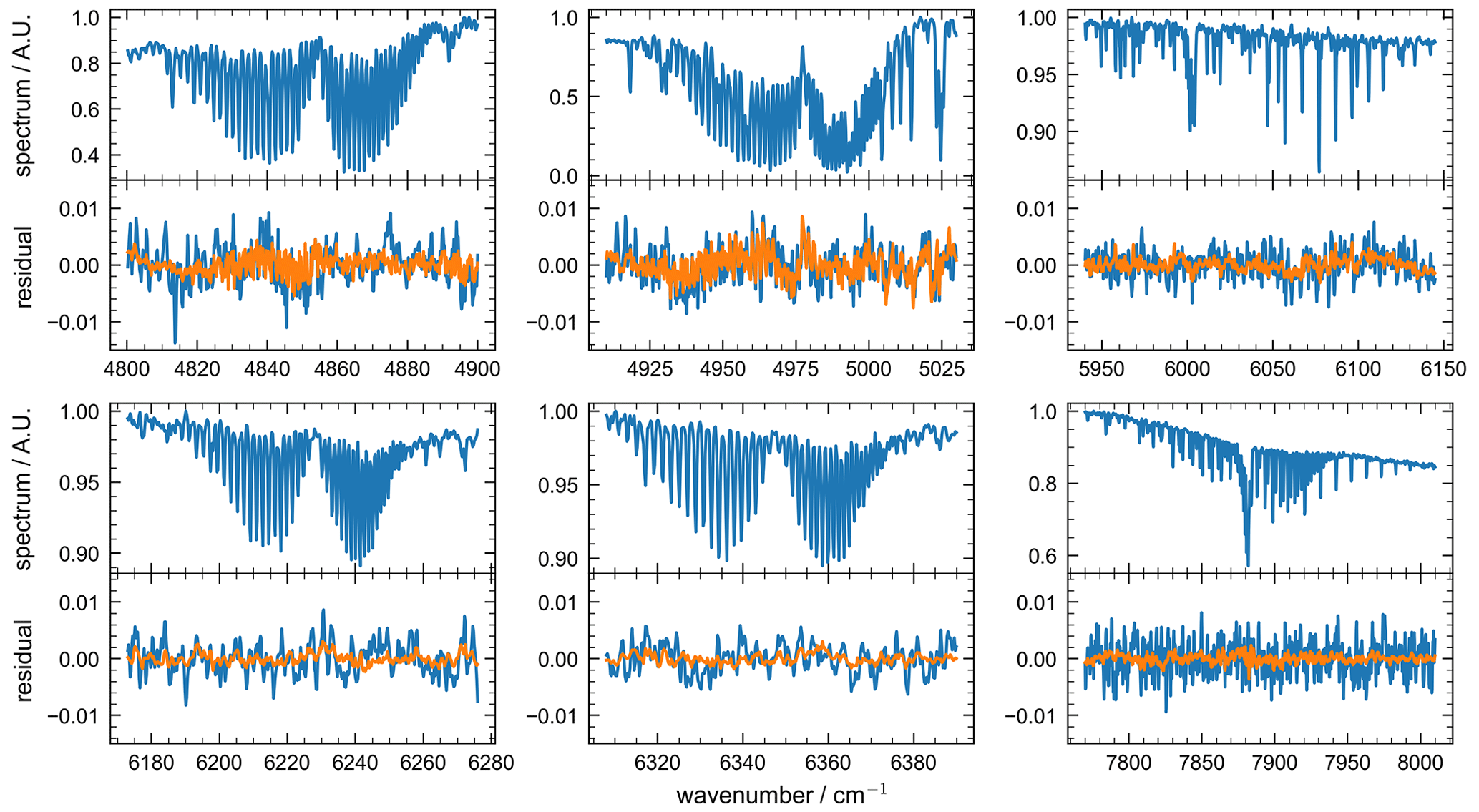
Figure 6Typical spectra (upper subpanels) and fit residuals (lower subpanels, measured minus simulated) for 5 min averages (blue) overlaid with residuals averaged over the whole measurement period (orange) for the six retrieval windows (panels) defined in Table 2. Spectra are scaled to the maximum intensity for each window.
Fitting the path-averaged temperature instead of imposing it from the weather station data yields a noticeable improvement in fit quality and results in more realistic temperature diurnal cycles. This is especially true in the early morning hours with substantial temperature gradients along the path. Most temperature information comes from the 2 µm windows (windows 1 and 2). The estimated path-averaged temperature is on average 0.7 K lower than the temperature at the weather station. We find that sensitivity studies neglecting line mixing in the 2 µm windows (windows 1 and 2) resulted in path-averaged temperature estimates that were low-biased by 2 to 6 K with respect to the weather station records. This bias is consistent with the findings of Griffith et al. (2018), who neglected line mixing and found similar low-biased path-averaged temperature information. Thus, consideration of spectroscopic line-mixing effects is required to accurately represent the actual path-averaged temperature and to improve on fit quality.
3.2 Precision of target gas CDs and dry-air mole fractions
Table 3 lists the relative precision for CO2 and CH4 CDs and their dry-air mole fractions xCO2 (2.5 ppm, 0.58 %) and xCH4 (18 ppb, 0.89 %) inferred by ratioing the target gas CDs with the measured O2 CDs. The precisions for dry-air mole fractions are comparable to those achieved by Griffith et al. (2018) (1.7 ppm for xCO2 and 23 ppb for xCH4), while they are substantially less precise than Deutscher et al. (2021) (0.28 ppm for xCO2 and 2.1 ppb for xCH4; 3 min measurements). Deutscher et al. (2021) mostly achieved this through a fixed connection of the FTS instrument and telescope, replacing the fiber coupling with a mirror and beam-splitter setup that allows for significantly higher optical throughput by more than an order of magnitude, substantially improving the spectral SNR and hence the precision of the retrieved trace gases. Due to size and weight, this type of configuration is not possible when using the IFS 125 HR FTS. Also, we only find minor changes in precision for xCO2 and xCH4 for the different settings listed in Table 1, even though the measurements differ significantly in spectral SNR due to different temporal and spectral resolution. The 1 min measurements show the same precisions for target gases once averaged on the same 5 min timescale, showing that the precision is not dominated by real fluctuations during the time of a single measurement. The high-resolution measurements show the same target gas precisions as the low-resolution counterparts. Since the line depth is mostly dominated by the ILS for the low-resolution parameters, it increases with higher resolution and compensates for the worse spectral SNR.
Table 3Relative precisions of measured total CDs and dry-air mole fractions for retrieved species.
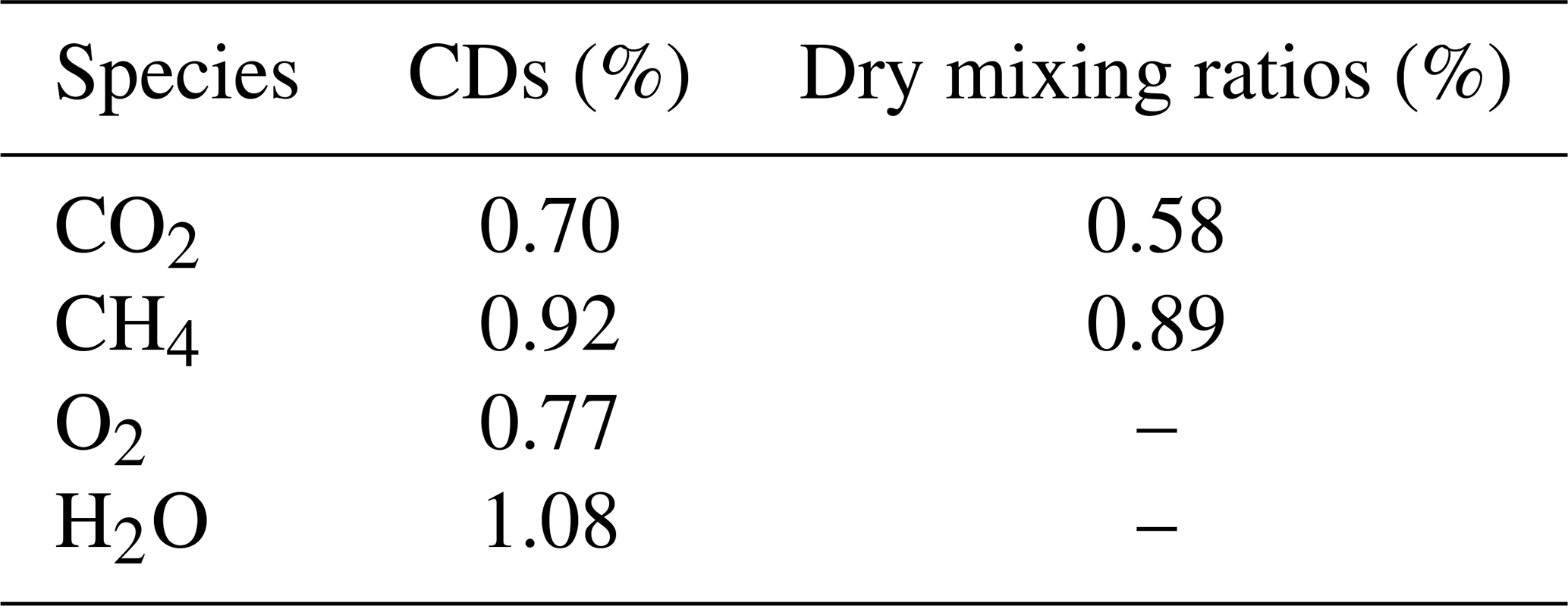
Interestingly, our dry-air mole fractions show a slightly higher level of precision than the respective CDs. We conclude that there is a systematic effect, which affects all retrieved CDs by a common similar factor. This systematic effect then at least partially cancels when dividing the target gas CDs by the measured O2 CDs. A candidate for causing such an effect could be changes in the refractive index along the light path during the recording of the interferograms. These changes induce slight variations of the transmittance of the optical system with time and effectively function as a modification to the apodization function, slightly altering the ILS. Hence, calculating the dry-air mole fractions by dividing the target gas CDs by the O2 CDs retrieved from the same measurement partially compensates for this effect.
As expected, the dry air masses calculated via Eq. (2) way show significantly higher precision then using measured O2 CDs (0.089 % instead of 0.77 %). But this is reversed if we look at the precision of the dry-air mole fractions calculated from these air masses: for example, for CO2, where the total CD is measured to a precision of 0.70 %, the dry mixing ratios calculated via Eq. (1) show a precision of 0.58 %, while calculating via Eq. (2) yields 0.73 %. So when dividing with the uncorrelated but highly precise calculated total air masses, the noise propagates as expected and results in less precise dry-air mole fractions. This strengthens the argument that both the CO2 (or CH4) CD and the O2 CD are affected by systematic noise, which at least partially cancels out when dividing one by the other.
3.3 Time series of CO2 and CH4
Figure 7 shows the time series of the dry-air mole fractions xCO2 and xCH4 after bias correction and filtering low signal measurements (for example due to fog or dense rain). From 6 February until 11 July we achieve data coverage of 78 % for 10 min intervals. Months in which the instrument could be fully dedicated to the open-path measurements achieve even better coverage of up to 92 % in June. We find good agreement between open-path and in situ data. Both records reveal a decrease in the background xCO2, especially from mid-April onwards, as expected from enhanced biospheric activity in the Northern Hemisphere in spring and summer. On top of this large-scale trend, the signal is dominated by the diurnal cycle with regular nighttime enhancements and by events related to regional and local emissions and transport patterns. The two records also agree well for xCH4, but the time series show less regular diurnal cycle structures. For both gases, the open-path data show greater scatter than the in situ data as expected from the precision estimates.
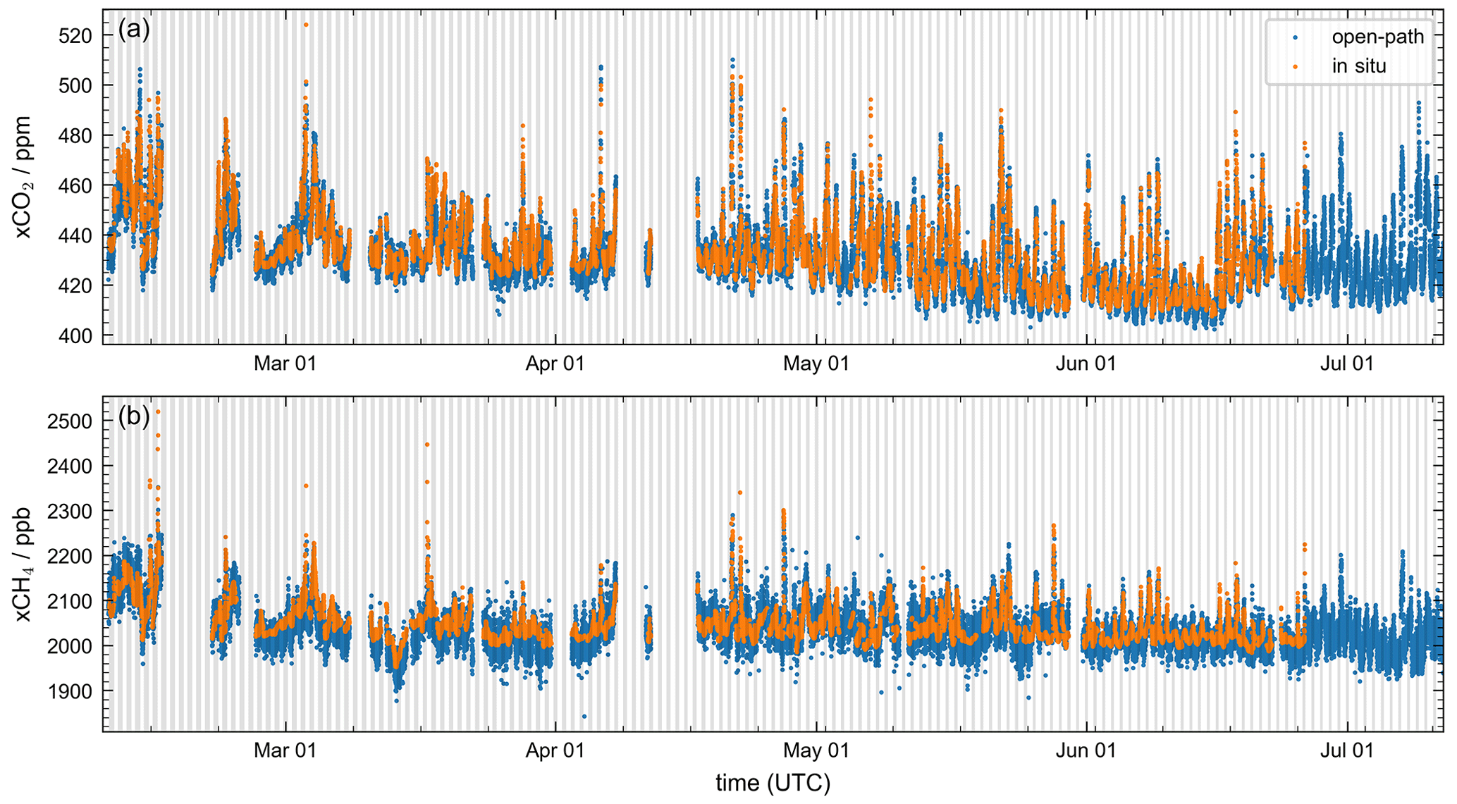
Figure 7Comparison between open-path (blue) and in situ (orange) measurements for dry mole fractions of CO2 (a) and CH4 (b). The open-path data shown cover the period from 6 February until 11 July, including gaps of a few days. In situ measurements were available until 26 June.
Figure 8 shows the statistics of the differences between the open-path and in situ records of xCO2 and xCH4. While the majority of the differences center around zero with a spread that corresponds to the precision of the records, the statistics show a significant tail for xCO2, with the in situ data being larger than the open-path data.
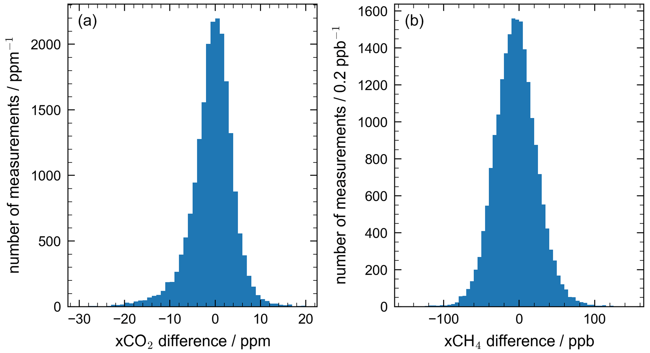
Figure 8Difference between the two instruments (open-path minus in situ) for xCO2 (a) and xCH4 (b). A clear central peak around 0 is visible for both gases. For xCO2, measurements where the two instruments significantly deviate from each other tend to bias towards lower values, so lower concentrations were measured by the open-path system and higher concentrations were measured by the in situ system. For xCH4, there is no significant bias.
While the records largely agree, Fig. 9 shows events for xCO2, and to an extent for xCH4, during which the open-path and in situ data differ. In the period 17 to 19 March in situ and open-path data align during the day but differ by up to 20 ppm in xCO2 during the night, while no noticeable difference is present in the xCH4 records. Both of these nights have in common that the predominant wind direction (as measured at the institute) is from the southeast (135∘). Figure 10 shows the differences between open-path and in situ data plotted over wind direction. The distribution indeed shows a systematic difference in xCO2 for wind directions around 135∘ with a gentle decline in the differences towards winds from the east and a relatively sharp transition towards winds from the south. The city center of Heidelberg at the mouth of Neckar river valley is located at around 135∘. One hypothesis is that in this wind situation the residential area below the open path is flushed with CO2-poor air from the river valley due to a deflection of air masses when exiting the Neckar valley, while the in situ station still samples CO2-rich urban air masses. We found around 10 nights showing this predominant steady wind situation, all of them in February and March. All but one show the described enhancement of in situ over open-path measurements. There are no daytime observations of this phenomenon, since this wind situation only occurs at nights, driven by the topography of the wide and flat Rhine valley and the hills in the east. This invites further research on whether high-resolution meteorological models can represent such effects and what the representativeness of the open-path and in situ records is.
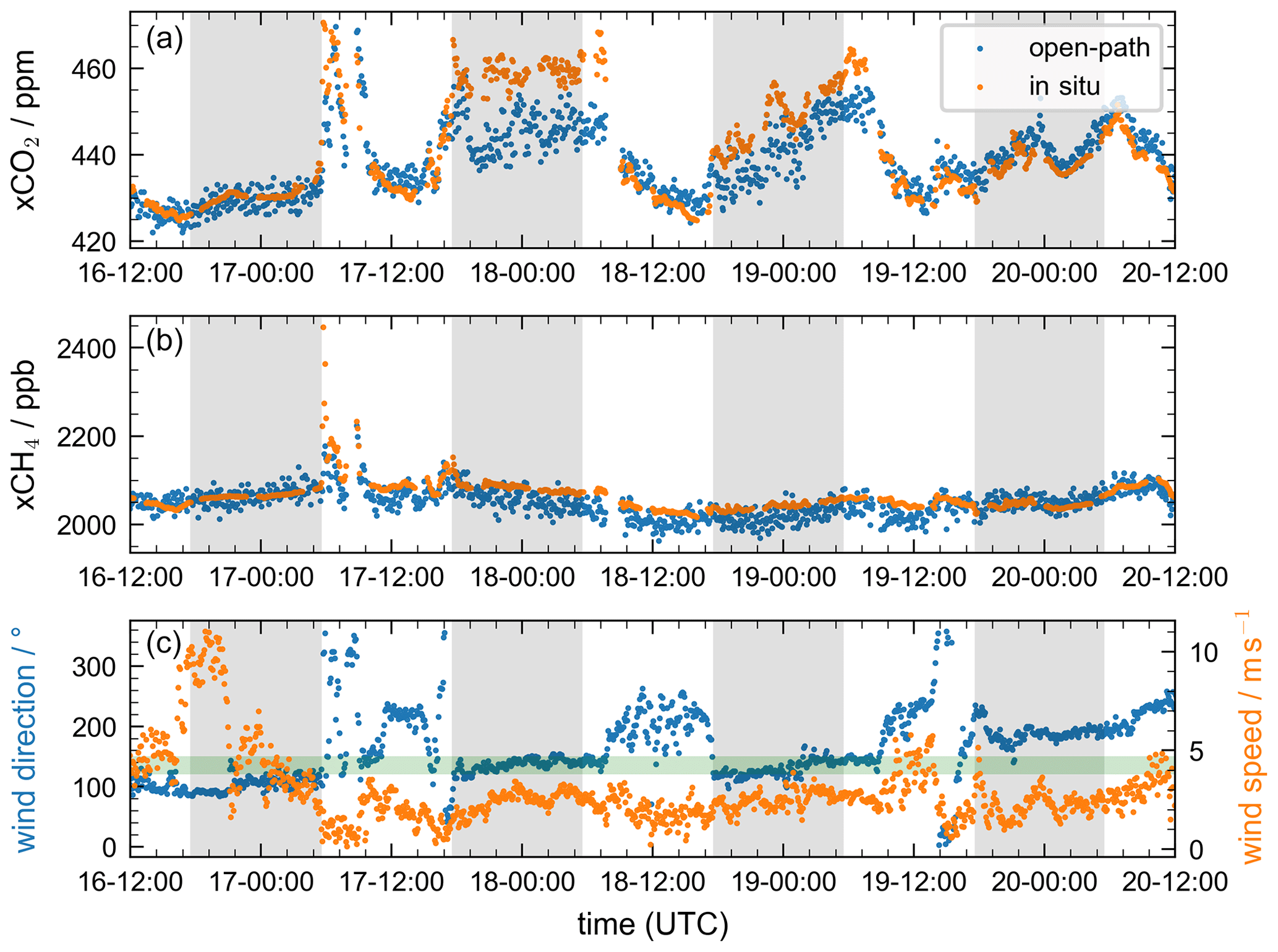
Figure 9Events of interest from 16 to 20 March 2023. On 17 March, shortly after sunrise, xCH4 (b) increases by several hundred parts per billion in a sharp spike for the in situ measurement (orange), but only by a fraction of that for the open-path (blue). Further, during the two subsequent nights the in situ records show a significant enhancement over the open-path instrument for the measured xCO2 (a). For both of these latter events, the wind direction (c, blue) is quite steady at around 135 ± 15∘ (green horizontal band). The wind speed (c, orange) does not show any remarkable features during this time.
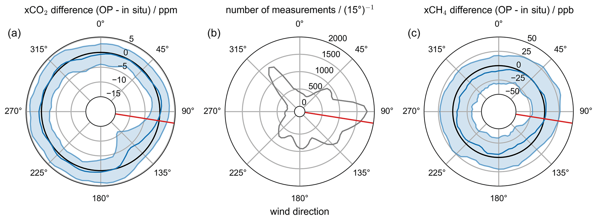
Figure 10Difference between the two instruments (open-path minus in situ) for xCO2 (a) and xCH4 (b) depending on wind direction. Plotted differences are averages over all measurements which have wind directions within a ± 15∘ arc and a wind speed above 1 ms−1. The blue band gives the 1-sigma percentile of the distribution. The red line indicates the viewing direction of the open-path system. An obvious feature for the wind direction from approximately 135∘ is visible for xCO2, but not for xCH4. The open-path system measures significantly lower values on average for xCO2 than the in situ system for wind coming from the southeast.
For xCH4, the picture is less clear. For most wind directions, the in situ instrument measures slightly higher xCH4 concentrations than the open-path instrument. The most notable feature is a peak of relatively higher open-path concentrations for winds from the east and northeast. All of this, however, is barely significant. In time series, differences in xCH4 typically show up in the form of sharp emission spikes which are covered by both instruments to a different extent, most likely due to a local source location. The largest sources of CH4 in the area are leakages from the natural gas distribution system and emissions from the sewer system (Wietzel, 2021). It seems reasonable that the open-path system, with its larger area footprint, would see such emissions on a more regular basis than the in situ instrument and, if the in situ instrument is located within such an emission plume, that the total enhancement is more diluted in the total CD measured by the open-path system. A detailed assessment of such differences, however, requires local modeling of air mass transport.
Figure 11 shows the diurnal cycles for xCO2 for weekends and weekdays averaged over the entire reported period. There is a clear difference between weekends and weekdays for the morning hours, which is related to CO2 exhaust from traffic being emitted into a shallow morning boundary layer during weekdays but not during weekends. The enhancement in the morning amounts to roughly 5 ppm, while the afternoon rush hour results in smaller enhancements since boundary layer mixing processes are more effective in the afternoon than in the morning. Comparing the in situ and open-path data, the agreement is excellent for the weekends with average differences of less than 1 ppm during the day and slightly larger differences during night. On the weekdays, however, the in situ data rather systematically indicate 1 to 2 ppm greater xCO2 than the open-path data. This might point to a local signal that contributes more to the in situ samples which is not represented on the 1.5 km averaging scale of the open-path experiment. While such representativeness issues might appear small, they become important when aiming at quantification and verification of local emissions with atmospheric models.
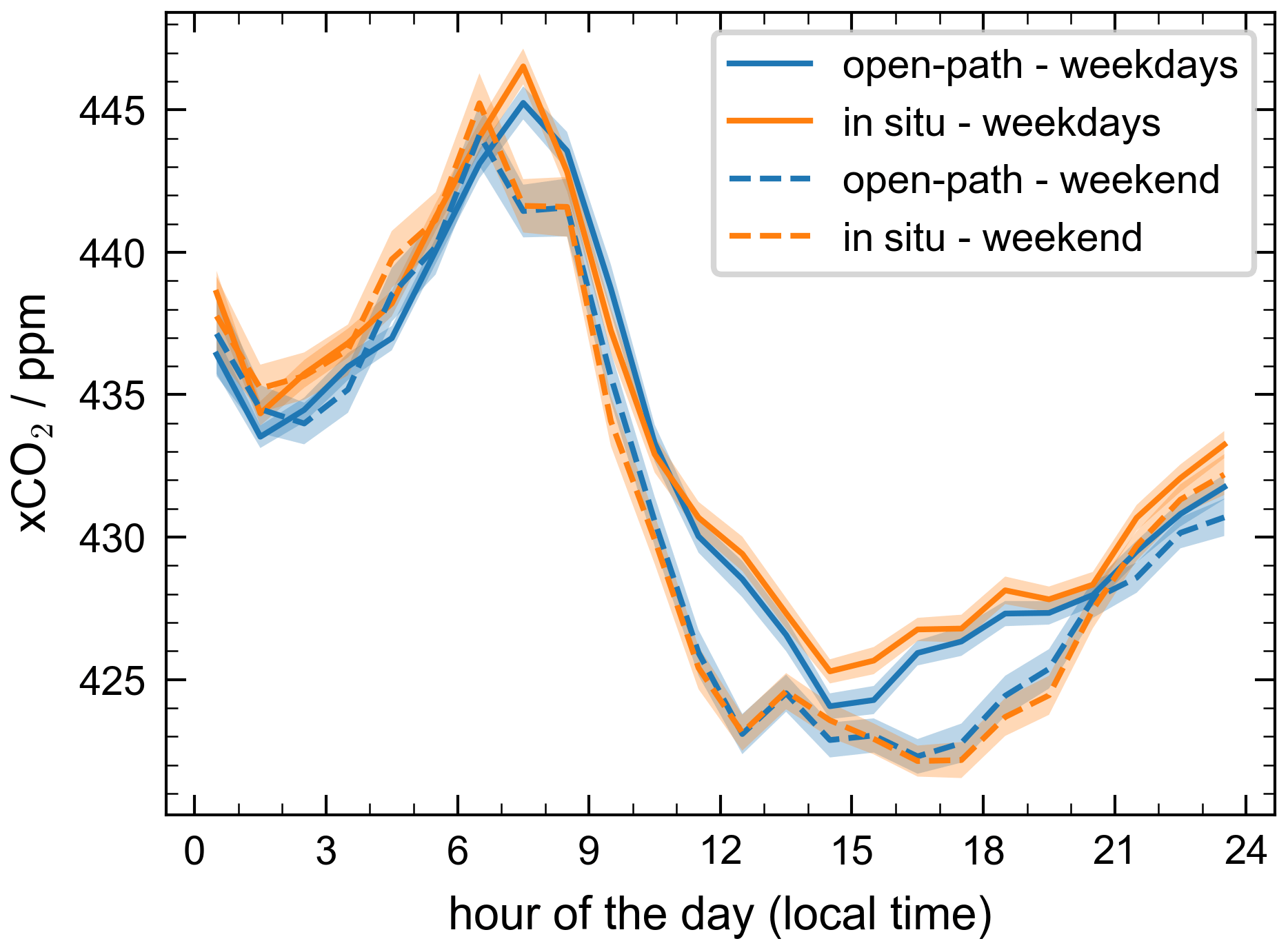
Figure 11Diurnal cycle of xCO2 for weekdays (solid lines) and weekends (dashed lines). Open-path (blue) and in situ (orange) cycles are in good accordance on weekends. Shaded areas give a statistical 1-sigma confidence level of the mean. On weekdays, the in situ instrument systematically measures 1 to 2 ppm greater values than the open-path instrument.
We report on the successful development, setup, and performance evaluation of an open-path greenhouse gas observatory in the city of Heidelberg, Germany. The system is based on the IFS 125HR FTS manufactured by Bruker Optics, which makes our setup highly versatile regarding spectral resolution, as well as regarding detector options and hence spectral coverage. However, this choice of instrument does not provide the portability demonstrated by the setup of Deutscher et al. (2021). Our system mainly operates at a standard spectral resolution of 0.55 cm−1, with experiments run at 0.11 cm−1. The spacious and modular design of the FTS enables modulating the light beam coming from a halogen light source first, before the light beam travels across the 1.5 km path (one-way) above the city. Sending the interferograms instead of the unmodulated light beam along the absorption path enables measurements during day and night without the need to correct for scattered sunlight. Continuously operating since 8 February 2023, the observatory achieves precisions of 2.7 ppm (0.58 %) for xCO2 and 18 ppb (0.89 %) for xCH4 in 5 min measurements, which is comparable to the pilot study by Griffith et al. (2018) but less precise than the beam-splitter coupled setup by Deutscher et al. (2021). Over the whole period, we achieved data coverage of 78 % and even up to 92 % for months in which the FTS instrument could be fully dedicated to the open-path measurements. We found that it is important to consider spectroscopic line-mixing effects of CO2 in the 2 µm band to retrieve accurate path-average temperatures and that calculating the dry-air mole fractions xCO2 and xCH4 using co-measured O2 CDs partially compensates for systematic errors.
For the period from 8 February to 26 June 2023, we compared the open-path xCO2 and xCH4 abundances to in situ data measured at one end of the open-path arrangement at the IUP. First, we found an overall bias correction factor for the open-path data by scaling to the in situ data collected under background conditions. After bias correction, both records are in good agreement, both showing a similar interannual trend as well as diurnal cycles. Then, we focused on showing differences between the in situ and open-path records that most likely stem from the two methods being representative of different horizontal averaging scales. We found differences of up to 20 ppm in xCO2 under southeasterly wind directions, which suggests that the in situ data are more sensitive to localized source patterns than the open-path data. For xCH4, we detected a weak correlation of the differences with easterly winds, which remains unexplained so far. Examining the xCO2 diurnal cycles on weekends and weekdays, both the open-path and in situ methods show a clear signal from traffic emissions during the morning rush hour, but the in situ instrument reports slightly but systematically greater xCO2 mole fractions during weekdays. These are all indications that local emission and transport processes alter the difference between in situ and open-path measurements, which questions the representativeness of in situ data. Thus, we recommend evaluating our measurements against atmospheric models that operate at various horizontal resolutions. This can provide insights on how representative the in situ and open-path data are on grid scales inherent to the models used for quantifying and verifying urban emissions.
Building on the basic observatory setup discussed here and on the versatility of the IFS 125HR FTS, we will aim to refine and expand the technique in the future. Measuring species such as CO and NO2 together with CO2 might help attribute xCO2 patterns to specific combustion sources. CO observations are currently hindered by the weak transmittance of our cube-corner reflectors in the 2.3 µm range. Thus, replacing the cube corners will have priority. NO2 has absorption structures in the visible spectral range (0.40 to 0.48 µm), which is within the range of the silicon detector of our FTS. Previous studies have employed DOAS spectrometers to measure NO2 with a similar open-path arrangement as used here. We will also examine whether operating the FTS at higher spectral resolution improves the performance, for example by better separating the target spectral signatures from interfering absorption structures or by reducing systematic errors, e.g., due to ILS uncertainties. Open-path measurements might further prove an interesting tool to check and validate spectral line parameters by providing long absorption paths in a real but less complex atmosphere than direct-sun occultation measurements, which are typically used for these validations. Such checks might include the relative and absolute intensity of different absorption bands, but also temperature dependencies of line strengths and differences in pressure broadening by dry and wet air. Especially when analyzing such line-broadening effects, high-resolution measurements, which fully resolve the spectral line, should provide a clear advantage over lower-resolution measurements. For checking absolute intensity parameters, it might be necessary to look for more accurate ways to evaluate the bias compared to an in situ system. Long, continuous time series by our observatory provide a solid database for such validations. When it comes to improving on specificity for local emission attribution, we will consider expanding the observatory with additional absorption paths across the city such that the combination of paths yields some primitive horizontal mapping information.
The data are available from the corresponding author upon request.
TDS developed the open-path setup and carried out the formal data analysis. JK and SS supported the development with their experience in open-path measurements. RK supported the development in the lab. BAL supported the data analysis. MS provided the in situ measurements. SNV advised on the data analysis. FH supported the instrument developed, especially with his expertise in FTIR spectroscopy. DWTG supported the development with the experience and data from his pilot study. TDS and AB wrote the paper, and all authors commented on the draft. AB conceptualized the project.
At least one of the (co-)authors is a member of the editorial board of Atmospheric Measurement Techniques. The peer-review process was guided by an independent editor, and the authors also have no other competing interests to declare.
Publisher's note: Copernicus Publications remains neutral with regard to jurisdictional claims made in the text, published maps, institutional affiliations, or any other geographical representation in this paper. While Copernicus Publications makes every effort to include appropriate place names, the final responsibility lies with the authors.
Many thanks to Samuel Hammer, Susanne Preunkert, and Angelika Gassama for keeping the IUP weather station running reliably. Special thanks to Lukas Pilz for his relentless support and push for better software standards and practices, from which the quality of the software within this project profited a lot.
This research has been supported by the Deutsche Forschungsgemeinschaft (DFG, German Research Foundation (grant no. 414273072)).
This paper was edited by Haichao Wang and reviewed by three anonymous referees.
Bai, M., Flesch, T., Trouvé, R., Coates, T., Butterly, C., Bhatta, B., Hill, J., and Chen, D.: Gas Emissions during Cattle Manure Composting and Stockpiling, J. Environ. Qual., 49, 228–235, https://doi.org/10.1002/jeq2.20029, 2020. a
Bailey, D. M., Adkins, E. M., and Miller, J. H.: An Open-Path Tunable Diode Laser Absorption Spectrometer for Detection of Carbon Dioxide at the Bonanza Creek Long-Term Ecological Research Site near Fairbanks, Alaska, Appl. Phys. B, 123, 245, https://doi.org/10.1007/s00340-017-6814-8, 2017. a
Birk, M., Röske, C., and Wagner, G.: High Accuracy CO2 Fourier Transform Measurements in the Range 6000–7000 cm−1, J. Quant. Spectrosc. Ra., 272, 107791, https://doi.org/10.1016/j.jqsrt.2021.107791, 2021. a
Coddington, I., Newbury, N., and Swann, W.: Dual-Comb Spectroscopy, Optica, 3, 414, https://doi.org/10.1364/OPTICA.3.000414, 2016. a
Deutscher, N. M., Naylor, T. A., Caldow, C. G. R., McDougall, H. L., Carter, A. G., and Griffith, D. W. T.: Performance of an open-path near-infrared measurement system for measurements of CO2 and CH4 during extended field trials, Atmos. Meas. Tech., 14, 3119–3130, https://doi.org/10.5194/amt-14-3119-2021, 2021. a, b, c, d, e
Dobler, J., Braun, M., Blume, N., and Zaccheo, T.: A New Laser Based Approach for Measuring Atmospheric Greenhouse Gases, Remote Sens.-Basel, 5, 6284–6304, https://doi.org/10.3390/rs5126284, 2013. a, b
Fiehn, A., Kostinek, J., Eckl, M., Klausner, T., Gałkowski, M., Chen, J., Gerbig, C., Röckmann, T., Maazallahi, H., Schmidt, M., Korbeń, P., Neçki, J., Jagoda, P., Wildmann, N., Mallaun, C., Bun, R., Nickl, A.-L., Jöckel, P., Fix, A., and Roiger, A.: Estimating CH4, CO2 and CO emissions from coal mining and industrial activities in the Upper Silesian Coal Basin using an aircraft-based mass balance approach, Atmos. Chem. Phys., 20, 12675–12695, https://doi.org/10.5194/acp-20-12675-2020, 2020. a
Frey, M., Sha, M. K., Hase, F., Kiel, M., Blumenstock, T., Harig, R., Surawicz, G., Deutscher, N. M., Shiomi, K., Franklin, J. E., Bösch, H., Chen, J., Grutter, M., Ohyama, H., Sun, Y., Butz, A., Mengistu Tsidu, G., Ene, D., Wunch, D., Cao, Z., Garcia, O., Ramonet, M., Vogel, F., and Orphal, J.: Building the COllaborative Carbon Column Observing Network (COCCON): long-term stability and ensemble performance of the EM27/SUN Fourier transform spectrometer, Atmos. Meas. Tech., 12, 1513–1530, https://doi.org/10.5194/amt-12-1513-2019, 2019. a
Gordon, I., Rothman, L., Hargreaves, R., Hashemi, R., Karlovets, E., Skinner, F., Conway, E., Hill, C., Kochanov, R., Tan, Y., Wcisło, P., Finenko, A., Nelson, K., Bernath, P., Birk, M., Boudon, V., Campargue, A., Chance, K., Coustenis, A., Drouin, B., Flaud, J., Gamache, R., Hodges, J., Jacquemart, D., Mlawer, E., Nikitin, A., Perevalov, V., Rotger, M., Tennyson, J., Toon, G., Tran, H., Tyuterev, V., Adkins, E., Baker, A., Barbe, A., Canè, E., Császár, A., Dudaryonok, A., Egorov, O., Fleisher, A., Fleurbaey, H., Foltynowicz, A., Furtenbacher, T., Harrison, J., Hartmann, J., Horneman, V., Huang, X., Karman, T., Karns, J., Kassi, S., Kleiner, I., Kofman, V., Kwabia–Tchana, F., Lavrentieva, N., Lee, T., Long, D., Lukashevskaya, A., Lyulin, O., Makhnev, V. Yu., Matt, W., Massie, S., Melosso, M., Mikhailenko, S., Mondelain, D., Müller, H., Naumenko, O., Perrin, A., Polyansky, O., Raddaoui, E., Raston, P., Reed, Z., Rey, M., Richard, C., Tóbiás, R., Sadiek, I., Schwenke, D., Starikova, E., Sung, K., Tamassia, F., Tashkun, S., Vander Auwera, J., Vasilenko, I., Vigasin, A., Villanueva, G., Vispoel, B., Wagner, G., Yachmenev, A., and Yurchenko, S.: The HITRAN2020 Molecular Spectroscopic Database, J. Quant. Spectrosc. Ra., 277, 107949, https://doi.org/10.1016/j.jqsrt.2021.107949, 2022. a
Griffith, D. W. T., Pöhler, D., Schmitt, S., Hammer, S., Vardag, S. N., and Platt, U.: Long open-path measurements of greenhouse gases in air using near-infrared Fourier transform spectroscopy, Atmos. Meas. Tech., 11, 1549–1563, https://doi.org/10.5194/amt-11-1549-2018, 2018. a, b, c, d, e, f, g, h, i, j, k
Gurney, K. R., Liang, J., Roest, G., Song, Y., Mueller, K., and Lauvaux, T.: Under-Reporting of Greenhouse Gas Emissions in U. S. Cities, Nat. Commun., 12, 553, https://doi.org/10.1038/s41467-020-20871-0, 2021. a
Hall, B. D., Crotwell, A. M., Kitzis, D. R., Mefford, T., Miller, B. R., Schibig, M. F., and Tans, P. P.: Revision of the World Meteorological Organization Global Atmosphere Watch (WMO/GAW) CO2 calibration scale, Atmos. Meas. Tech., 14, 3015–3032, https://doi.org/10.5194/amt-14-3015-2021, 2021. a
Hartmann, J.-M., Tran, H., and Toon, G. C.: Influence of line mixing on the retrievals of atmospheric CO2 from spectra in the 1.6 and 2.1 µm regions, Atmos. Chem. Phys., 9, 7303–7312, https://doi.org/10.5194/acp-9-7303-2009, 2009. a
Hase, F., Blumenstock, T., and Paton-Walsh, C.: Analysis of the Instrumental Line Shape of High-Resolution Fourier Transform IR Spectrometers with Gas Cell Measurements and New Retrieval Software, Appl. Optics, 38, 3417, https://doi.org/10.1364/AO.38.003417, 1999. a
Hoheisel, A.: Evaluation of Greenhouse Gas Time Series to Characterise Local and Regional Emissions, PhD thesis, Heidelberg University, http://archiv.ub.uni-heidelberg.de/volltextserver/id/eprint/30321 (last access: 2 August 2023), 2021. a
Hoheisel, A., Yeman, C., Dinger, F., Eckhardt, H., and Schmidt, M.: An improved method for mobile characterisation of δ13CH4 source signatures and its application in Germany, Atmos. Meas. Tech., 12, 1123–1139, https://doi.org/10.5194/amt-12-1123-2019, 2019. a
Karman, T., Gordon, I. E., Van Der Avoird, A., Baranov, Y. I., Boulet, C., Drouin, B. J., Groenenboom, G. C., Gustafsson, M., Hartmann, J.-M., Kurucz, R. L., Rothman, L. S., Sun, K., Sung, K., Thalman, R., Tran, H., Wishnow, E. H., Wordsworth, R., Vigasin, A. A., Volkamer, R., and Van Der Zande, W. J.: Update of the HITRAN Collision-Induced Absorption Section, Icarus, 328, 160–175, https://doi.org/10.1016/j.icarus.2019.02.034, 2019. a
Kiel, M., Eldering, A., Roten, D. D., Lin, J. C., Feng, S., Lei, R., Lauvaux, T., Oda, T., Roehl, C. M., Blavier, J.-F., and Iraci, L. T.: Urban-Focused Satellite CO2 Observations from the Orbiting Carbon Observatory-3: A First Look at the Los Angeles Megacity, Remote Sens. Environ., 258, 112314, https://doi.org/10.1016/j.rse.2021.112314, 2021. a
Kochanov, R., Gordon, I., Rothman, L., Wcisło, P., Hill, C., and Wilzewski, J.: HITRAN Application Programming Interface (HAPI): A Comprehensive Approach to Working with Spectroscopic Data, J. Quant. Spectrosc. Ra., 177, 15–30, https://doi.org/10.1016/j.jqsrt.2016.03.005, 2016. a
Lamouroux, J., Tran, H., Laraia, A., Gamache, R., Rothman, L., Gordon, I., and Hartmann, J.-M.: Updated Database plus Software for Line-Mixing in CO2 Infrared Spectra and Their Test Using Laboratory Spectra in the 1.5–2.3 µm Region, J. Quant. Spectrosc. Ra., 111, 2321–2331, https://doi.org/10.1016/j.jqsrt.2010.03.006, 2010. a
Lian, J., Bréon, F.-M., Broquet, G., Zaccheo, T. S., Dobler, J., Ramonet, M., Staufer, J., Santaren, D., Xueref-Remy, I., and Ciais, P.: Analysis of temporal and spatial variability of atmospheric CO2 concentration within Paris from the GreenLITE™ laser imaging experiment, Atmos. Chem. Phys., 19, 13809–13825, https://doi.org/10.5194/acp-19-13809-2019, 2019. a
Malarich, N. A., Washburn, B. R., Cossel, K. C., Mead, G. J., Giorgetta, F. R., Herman, D. I., Newbury, N. R., and Coddington, I.: Validation of Open-Path Dual-Comb Spectroscopy against an O2 Background, Opt. Express, 31, 5042, https://doi.org/10.1364/OE.480301, 2023. a
Marcotullio, P. J., Sarzynski, A., Albrecht, J., Schulz, N., and Garcia, J.: The Geography of Global Urban Greenhouse Gas Emissions: An Exploratory Analysis, Climatic Change, 121, 621–634, https://doi.org/10.1007/s10584-013-0977-z, 2013. a
Merten, A., Tschritter, J., and Platt, U.: Design of Differential Optical Absorption Spectroscopy Long-Path Telescopes Based on Fiber Optics, Appl. Optics, 50, 738, https://doi.org/10.1364/AO.50.000738, 2011. a
Mueller, K. L., Lauvaux, T., Gurney, K. R., Roest, G., Ghosh, S., Gourdji, S. M., Karion, A., DeCola, P., and Whetstone, J.: An Emerging GHG Estimation Approach Can Help Cities Achieve Their Climate and Sustainability Goals, Environ. Res. Lett., 16, 084003, https://doi.org/10.1088/1748-9326/ac0f25, 2021. a
Nassar, R., Hill, T. G., McLinden, C. A., Wunch, D., Jones, D. B. A., and Crisp, D.: Quantifying CO2 Emissions From Individual Power Plants From Space, Geophys. Res. Lett., 44, 10045–10053, https://doi.org/10.1002/2017GL074702, 2017. a
Shusterman, A. A., Teige, V. E., Turner, A. J., Newman, C., Kim, J., and Cohen, R. C.: The BErkeley Atmospheric CO2 Observation Network: initial evaluation, Atmos. Chem. Phys., 16, 13449–13463, https://doi.org/10.5194/acp-16-13449-2016, 2016. a
Truong, G.-W., Waxman, E. M., Cossel, K. C., Baumann, E., Klose, A., Giorgetta, F. R., Swann, W. C., Newbury, N. R., and Coddington, I.: Accurate Frequency Referencing for Fieldable Dual-Comb Spectroscopy, Opt. Express, 24, 30495, https://doi.org/10.1364/OE.24.030495, 2016. a
United Nations Framework Convention on Climate Change (UNFCCC): The Paris Agreement, Treaty Section of the Office of Legal Affairs, United Nations Headquarters, New York, 2015. a
Waxman, E. M., Cossel, K. C., Truong, G.-W., Giorgetta, F. R., Swann, W. C., Coburn, S., Wright, R. J., Rieker, G. B., Coddington, I., and Newbury, N. R.: Intercomparison of open-path trace gas measurements with two dual-frequency-comb spectrometers, Atmos. Meas. Tech., 10, 3295–3311, https://doi.org/10.5194/amt-10-3295-2017, 2017. a
Waxman, E. M., Cossel, K. C., Giorgetta, F., Truong, G.-W., Swann, W. C., Coddington, I., and Newbury, N. R.: Estimating vehicle carbon dioxide emissions from Boulder, Colorado, using horizontal path-integrated column measurements, Atmos. Chem. Phys., 19, 4177–4192, https://doi.org/10.5194/acp-19-4177-2019, 2019. a
Wiacek, A., Li, L., Tobin, K., and Mitchell, M.: Characterization of trace gas emissions at an intermediate port, Atmos. Chem. Phys., 18, 13787–13812, https://doi.org/10.5194/acp-18-13787-2018, 2018. a
Wietzel, J. B.: Estimation of Methane Emissions in the Urban Area of Heidelberg by Mobile Measurements, Master's thesis, Heidelberg University, 2021. a
Wunch, D., Toon, G. C., Blavier, J.-F. L., Washenfelder, R. A., Notholt, J., Connor, B. J., Griffith, D. W. T., Sherlock, V., and Wennberg, P. O.: The Total Carbon Column Observing Network, Philos. T. R. Soc. A, 369, 2087–2112, https://doi.org/10.1098/rsta.2010.0240, 2011. a
You, Y., Moussa, S. G., Zhang, L., Fu, L., Beck, J., and Staebler, R. M.: Quantifying fugitive gas emissions from an oil sands tailings pond with open-path Fourier transform infrared measurements, Atmos. Meas. Tech., 14, 945–959, https://doi.org/10.5194/amt-14-945-2021, 2021. a