Ground-to-UAV, laser-based emissions quantification of methane and acetylene at long standoff distances

Cossel, Kevin C.; Waxman, Eleanor M.; Hoenig, Eli; Hesselius, Daniel; Chaote, Christopher; Coddington, Ian; Newbury, Nathan R.

doi:https://doi.org/10.5194/amt-16-5697-2023

Articles | Volume 16, issue 22

https://doi.org/10.5194/amt-16-5697-2023

Articles | Volume 16, issue 22

Research article

| Highlight paper

28 Nov 2023

Research article | Highlight paper |

| 28 Nov 2023

Ground-to-UAV, laser-based emissions quantification of methane and acetylene at long standoff distances

Kevin C. Cossel, Eleanor M. Waxman, Eli Hoenig, Daniel Hesselius, Christopher Chaote, Ian Coddington, and Nathan R. Newbury

Abstract

Determination of trace gas emissions from sources is critical for understanding and regulating air quality and climate change. Here, we demonstrate a method for rapid quantification of the emission rate of multiple gases from simple and complex sources using a mass balance approach with a spatially scannable open-path sensor – in this case, an open-path dual-comb spectrometer. The open-path spectrometer measures the total column density of gases between the spectrometer and a retroreflector mounted on an uncrewed aerial vehicle (UAV). By measuring slant columns at multiple UAV altitudes downwind of a source (or sink), the total emission rate can be rapidly determined without the need for an atmospheric dispersion model. Here, we demonstrate this technique using controlled releases of CH₄ and C₂H₂. We show an emission rate determination to within 56 % of the known flux with a single 10 min flight and within 15 % of the known flux after 12 flights. Furthermore, we estimate the detection limit for CH₄ emissions to be 0.03 g CH₄ s⁻¹. This detection limit is approximately the same as the emissions from 25 head of beef cattle and is less than the average emissions from a small oil field pneumatic controller. Other gases including CO₂, NH₃, HDO, ethane, formaldehyde (HCHO), CO, and N₂O can be measured by simply changing the dual-comb spectrometer.

Download & links

Article (PDF, 4148 KB)

Download & links

How to cite

How to cite.

Dates

Received: 08 Apr 2023 – Discussion started: 24 Apr 2023 – Revised: 15 Sep 2023 – Accepted: 02 Oct 2023 – Published: 28 Nov 2023

1 Introduction

Measurements of the emission rate of a gas or gases from point and area sources are important in a range of monitoring applications. Several examples include measurement of emissions of CH₄ and volatile organic compounds (VOCs) from oil and gas facilities (well pads, compressor stations, processing plants, etc.) as well as from landfills and composting facilities; CH₄ and N₂O (as well as VOCs) from wastewater treatment plants; CH₄, NH₃, and N₂O from agricultural sites; and VOCs from industrial facilities. In all these examples, there are several important challenges for a measurement system. First, it is desirable to be able to measure emissions of multiple gases simultaneously. Second, the measurement system should be able to handle complex sources such as distributed sources or colocated sources. Finally, it is often desirable to be able to rapidly survey different sources to determine if emissions are present and then to quantify the emissions.

Because of the fundamental importance of emission rate measurements in monitoring and regulation, there is a wide range of different measurement methods that have been developed, all with distinct advantages and disadvantages. We cannot exhaustively review all the techniques here, but instead highlight a few general classes of techniques. The first are ground-based survey techniques with a point sensor (Vaughn et al., 2017; Zhang et al., 2019; Ravikumar et al., 2019; Riddick et al., 2022). One limitation of these techniques is that the vertical distribution of the gas is not measured, so assumptions need to be made about the vertical and horizontal gas dispersion (using an atmospheric transport model). The transport assumptions can be removed by releasing a tracer gas colocated with the unknown emission source (Czepiel et al., 1996; Mønster et al., 2014; Roscioli et al., 2015); however, this requires access to and knowledge of the emission source. To circumvent these challenges, mass balance approaches can be used by measuring in two dimensions, which greatly relaxes the requirements for the transport model. Most frequently, mass balance is performed using point sensors on aircraft (White et al., 1976; Alfieri et al., 2010; Karion et al., 2013; Conley et al., 2017). While effective for large sources, challenges such as flight altitude restrictions, cost, and the requirement for fast sensors can limit applicability and repeat measurements. More recently, uncrewed aerial vehicles (UAVs) have been used for small-scale mass balance (Golston et al., 2018; Gålfalk et al., 2021; Zondlo, 2021; Reuter et al., 2021), although not many sensors meet the precision or size, weight, and power requirements to deploy in this fashion. Long open-path measurements to a UAV were very recently used in conjunction with a Gaussian plume model to determine an emission rate from a point source (Soskind et al., 2023). Finally, several mass balance approaches have been demonstrated using column-integrated measurements including solar occultation flux (which can only be used during daytime or sunny conditions) (Mellqvist et al., 2010; Kille et al., 2017) and airborne lidar (which has focused on methane or carbon dioxide) (Ravikumar et al., 2019; Amediek et al., 2017; Bell et al., 2022; Kunkel et al., 2023; Johnson et al., 2021). There are two significant distinctions between these lidar approaches and the approach discussed here. First, lidar systems are mounted on a larger aircraft, which has added cost and complications but does not require a van and can more easily cover a large area. Second, lidar targets a single species, which is well suited to finding methane leaks in an oil or gas field, for example, while the system here relies on broadband dual-comb spectroscopy that can detect multiple species. If used in conjunction with a mid-infrared dual-comb system, this approach could then simultaneously detect multiple volatile organic compounds beyond methane.

Here, we demonstrate a new mobile micrometeorological mass balance method using a line-integrated sensor (in this case, open-path dual-comb spectroscopy or DCS) in combination with an uncrewed aerial vehicle. This is accomplished by measuring slant columns to a moving UAV that carries a small retroreflector downwind of an emission source as shown in Fig. 1. We test this technique using controlled releases of CH₄ and C₂H₂ from both a point source and a small area. A key strength of this technique – and other mass balance techniques – is that it does not rely on a dispersion model. In principle this approach is also compatible with any open-path laser measurement, such as tunable diode laser spectroscopy (Plant et al., 2015; Bailey et al., 2017; Dobler et al., 2017; Bai et al., 2022), but here we use a frequency comb to allow for simultaneous multispecies detection (Coddington et al., 2016; Cossel et al., 2021; Picqué and Hänsch, 2019). For example, while CH₄ and C₂H₂ measurements are demonstrated here, open-path dual-comb spectroscopy has been used to retrieve a host of interesting species including CO₂, NH₃, HDO, ethane, formaldehyde (HCHO), CO, and N₂O (Waxman et al., 2017; Ycas et al., 2019; Giorgetta et al., 2021; Herman et al., 2021).

2 Experimental setup

This method builds on our previous demonstration of spatially scanned DCS (Cossel et al., 2017), which is summarized in Fig. 1a. The primary components of the system (Fig. 1b) are the dual-frequency combs, a transmit–receive terminal that sends light over a long open-air path, and a mobile reflector on a quadcopter.

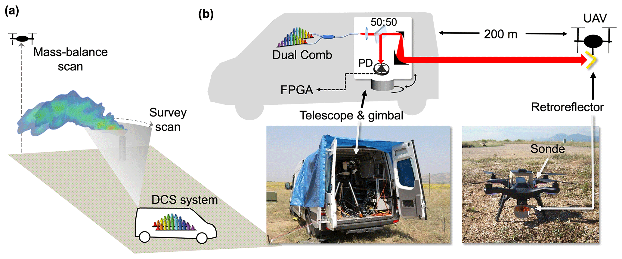
https://amt.copernicus.org/articles/16/5697/2023/amt-16-5697-2023-f01

Figure 1(a) Overview of the experimental concept. The DCS system measures integrated slant columns to a moving UAV. By performing survey scans, the presence and angular position of an emissions source can be rapidly determined. Mass balance scans downwind of the source then enable quantification of the emissions. (b) Details of the experimental setup. Light from the dual-frequency combs is combined in fiber, then launched out of a transmit–receive telescope system located on an azimuth–elevation gimbal to a retroreflector located on a UAV at a typical distance of 200 m. The return light from the retroreflector is separated with a 50:50 beam splitter and measured on a photodetector (PD). This signal is digitized and averaged with a field-programmable gate array (FPGA)-based acquisition system. The lower part of (b) shows the van in the field as well as a photo of the UAV with the retroreflector and sonde (see also Appendix A.)

Download

Here, we use robust erbium-doped fiber-based frequency combs operating in the near-infrared (Waxman et al., 2017). The design and operation of these combs have been described in detail previously (Truong et al., 2016). Briefly, the frequency combs have a nominal repetition rate of 200 MHz and a repetition rate difference of δf_rep= 625 Hz. The combs are both stabilized to a crystal oscillator and continuous-wave reference laser at 1560 nm to maintain mutual coherence between the combs. After amplification, spectral broadening, and spectral filtering to cover bands for C₂H₂ (1520–1540 nm) and CH₄ (1610–1670 nm), the light from the two combs is combined in fiber and then launched from a transmit–receive telescope (76.2 mm diameter aperture) to a retroreflector (62.5 mm diameter) located on a UAV (here, a quadcopter). Return light from the retroreflector is collected with the same telescope and reflected off a 50:50 beam splitter to a photodetector. Alignment with the retroreflector is maintained by an image-processing-based pointing servo using an 850 nm LED and Si CMOS camera co-aligned with the main telescope (Cossel et al., 2017). The return power was typically 100–200 µW with 10 %–20 % power fluctuations between each measured spectrum as well as larger “dropouts” and power drifts due to alignment issues such as sudden UAV movement or yaw of the UAV. These dropouts were usually < 10 % of a single flight. Figure 1b shows a more detailed view of the UAV. In addition to the retroreflector, the UAV also carries several sondes to measure temperature, pressure, humidity, and GPS location, as well as real-time kinematic (RTK) GPS for high-precision relative GPS location of the UAV. However, sufficient location precision was provided by the onboard GPS, so that is used for most of the data presented here. For field operations, the DCS system is housed in a van and connected via fiber to a telescope and fast azimuth–elevation gimbal located at the back of the van as pictured in Fig. 1b. Wind speed and direction were measured with a 3D sonic anemometer located away from the van at ∼ 2 m above ground. Additional meteorological parameters (temperature, pressure, independent wind speed and direction) were recorded by a weather station with a 2D sonic anemometer located above the van roof. This second wind measurement was used for redundancy and to verify the 3D sonic measurements. Finally, we measured CH₄ concentrations with a commercial cavity ring-down spectrometer (CRDS) that sampled air from above the roof of the van. This spectrometer was calibrated at the NOAA Global Monitoring Laboratory to provide WMO-traceable CH₄ measurements, which we use to determine the background CH₄ concentration during flights.

The dual-comb signal on the receive photodetector is a time domain interferogram (IGM) that repeats at a rate of δf_rep. We digitize this signal and co-add using a field-programmable gate array (FPGA). Sequential sets of 10 000 IGMs are co-added (with phase correction applied to each set of 100 sequential IGMs). In total this gives a 16 s sampling period. In post-processing, each saved IGM was converted to a transmission spectrum (Fig. 2a) via a Fourier transform and then fit with a spectral transmission model (calculated from HITRAN2008 using the measured temperatures and pressures; Rothman et al., 2009) plus a piecewise polynomial baseline term to determine total column densities for three gases: CH₄, H₂O, and C₂H₂ along the laser path, ${\overline{ρ}}_{g} = \int_{0}^{L} ρ (x, y, z) d r$ , where $ρ_{g} (x, y, z)$ is the spatially varying density of the gas, r is the position along the path, and dr is the differential path length (Waxman et al., 2017; Cossel et al., 2021). These total column densities are converted to path-averaged dry mixing ratios for CH₄ and C₂H₂ reported in parts per million (ppm) (µmol mol⁻¹) or parts per billion (ppb) (nmol mol⁻¹) using the temperature and pressure from the weather station, the temporally varying path length determined from the UAV GPS location, and the DCS-measured water vapor for the dry-air correction (Waxman et al., 2017). The measurement precision is characterized by the Allan–Werle deviation of the retrieved path-averaged concentration during one flight with no gas release (thus approximately uniform mixing ratios) as shown in Fig. 2b. For this flight, the number of co-added interferograms was reduced to 2500, resulting in measurements every 4 s. At the typical measurement time of 16 s, the CH₄ precision is around 23 ppm m (57 ppb for a round-trip path length of 400 m). This performance is similar to that obtained from Waxman et al. (2017) – 50 ppb extrapolated to the same measurement time and path length – indicating very little degradation due to motion of the UAV.

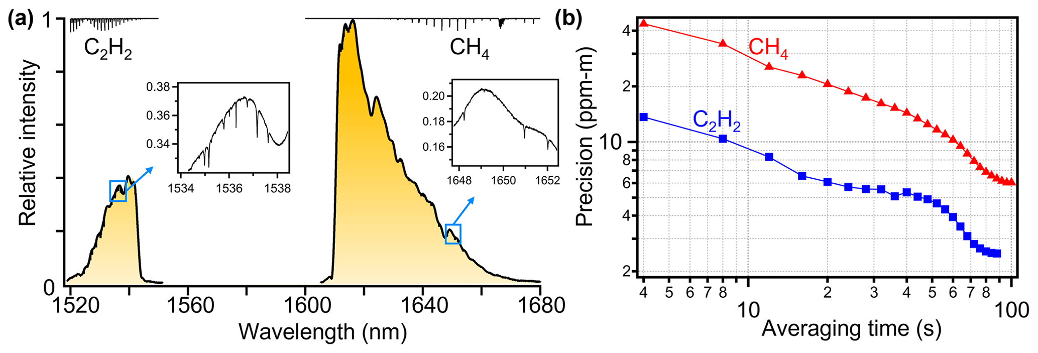
https://amt.copernicus.org/articles/16/5697/2023/amt-16-5697-2023-f02

Figure 2(a) Example normalized transmission spectrum (10 min average). C₂H₂ is retrieved in the band around 1540 nm and CH₄ is retrieved in the band around 1640 nm. A simulated transmission spectrum for both gases is shown along the top to guide the eye. The slower undulating structure in the spectra is stable over short times and results from the supercontinuum generation and spectral etalons in the system. (b) Allan deviation of ${\overline{ρ}}_{g}$ for both CH₄ and C₂H₂ at ambient concentration from one flight. The round-trip path length was around 400 m.

Download

Flights were performed across 4 different days. Each flight had a maximum duration of ∼ 10 min. Several different flight patterns were used; here we focus on horizontal and vertical scans. The UAV was manually piloted for all the flights. Several different leak locations and arrangements were used in order to mimic emission sources that might be observed in the field. Controlled releases of CH₄ and C₂H₂ were located ∼ 100 m from the van and were conducted using cylinders whose flow rate was either controlled with a mass flow controller or monitored with a flowmeter (see Appendix A for details). For CH₄, the flow rate was set to around 0.22 g s⁻¹. For C₂H₂, the flow rate was set to around 0.18 g s⁻¹ but was only used during a subset of releases. These flow rates correspond to a leak of ∼ 0.7 kg h⁻¹ for methane, corresponding to a practical lower bound for systems detecting methane leaks in oil and gas fields (Ravikumar et al., 2019; Johnson et al., 2021; Bell et al., 2022). The flow rate for acetylene was chosen to provide a similar signal level; future tests with multiple species would be coupled with the required species-dependent sensitivity. After the flowmeter or controller, the gas was sent through a piece of PTFE tubing a few meters long whose end was located between 0 m and ∼ 5 m above ground level to simulate a point source emission. Small-area diffuse emissions were also simulated by puncturing the PTFE tubing every ∼ 30 cm and placing the tubing on the ground across a ∼ 2 m diameter area.

3 Results

3.1 Survey scan for emissions detection

We first demonstrate rapid detection of an emission source and later quantification of its emissions. For detection, the UAV is scanned horizontally at 200 m distance from the telescope – as illustrated by the dotted grey line in Fig. 1a – resulting in measurements across a series of nearly horizontal slant paths. For this demonstration, the source emitted both CH₄ and C₂H₂ from a pole ∼ 5 m above ground level (AGL) located ∼ 100 m away from the launch–receive telescope.

To analyze the results, we calculate the path-averaged enhanced column density ( $Δ {\overline{ρ}}_{g}$ ) for each gas g (CH₄ and C₂H₂), $Δ {\overline{ρ}}_{g} = {\overline{ρ}}_{g} - L 〈 ρ_{g} 〉$ , where ${\overline{ρ}}_{g}$ is the measured column density, L is the path length, and 〈ρ_g〉 is the mean background concentration. For CH₄, the background concentration is obtained from the dry mixing ratio from the CRDS using the known air temperature, pressure, and water vapor interpolated to the DCS data timestamp. For C₂H₂, the background concentration is set to the mean of the DCS measurements without any release. Figure 3b shows the CH₄ and C₂H₂ path-averaged concentration enhancement ( $Δ {\overline{ρ}}_{g} / L)$ from a single flight consisting of two horizontal scans at different altitudes (scans at both altitudes are aggregated in one plot). As expected, we observe significant enhancements of CH₄ and C₂H₂ for slant paths when the UAV is immediately downwind of the emission location. The enhancements persist but decrease in amplitude as the paths move further downwind. Once the presence of an emissions source is detected with a horizontal scan, additional flights can be used for emissions quantification as discussed below. Further localization can be accomplished with more complex flight patterns (Soskind et al., 2023).

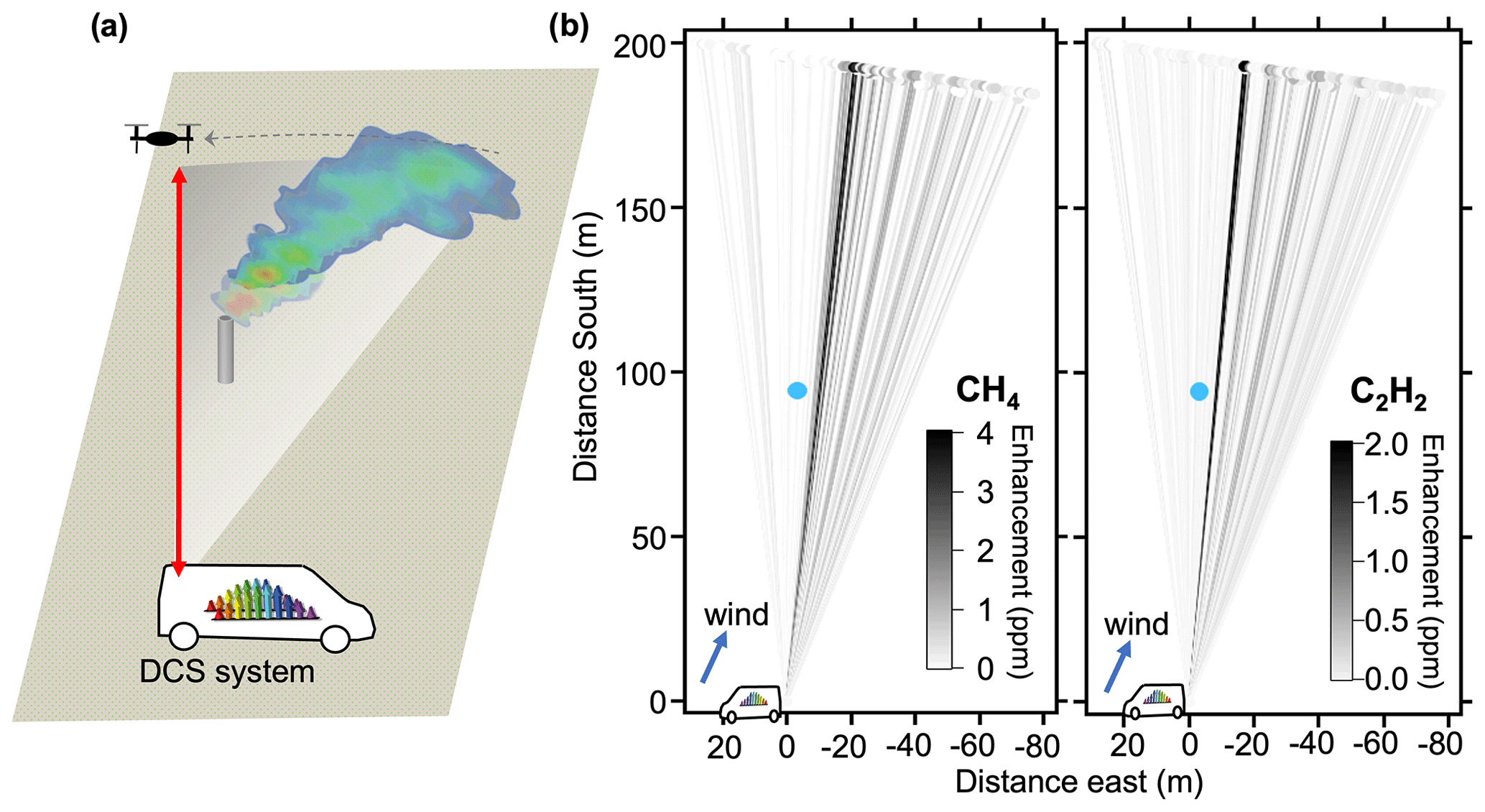
https://amt.copernicus.org/articles/16/5697/2023/amt-16-5697-2023-f03

Figure 3(a) Detection and location concept using a constant altitude horizontal scan. (b) Map of the results for CH₄ (left) and C₂H₂ (right) from a flight with both CH₄ and C₂H₂ releases. The van is located at (0, 0) and the UAV relative position is shown by the dots. For this flight, two horizontal scans were completed at 5 m and 9 m a.g.l. The release location is shown by a blue dot, and the wind direction is shown by a blue arrow. The release was at a height of ∼ 2 m a.g.l., and the mean wind speed was 2 m s⁻¹. Each measurement path is shown by a solid line, shaded by the path-averaged CH₄ or C₂H₂ enhancement over background (see text for details). For both gases, a sudden increase in the enhancement is visible ∼ 5 m downwind of the leak source.

Download

3.2 Mass balance scan for emissions quantification

3.2.1 Methods

In order to perform emissions rate quantification, the UAV flew a vertical profile downwind of the emissions source as illustrated in Fig. 4a. An example altitude profile recorded by the GPS on board the UAV is shown as an inset. In this case, two vertical profiles between ∼ 2 and 30 m above ground level were performed during a single flight. Flights were also conducted with a single vertical scan during the flight. The flight patterns result in a series of measurements of the column density (or path-integrated concentration), ${\overline{ρ}}_{g} (z)$ , for each gas species g and UAV height z with 16 s integration times.

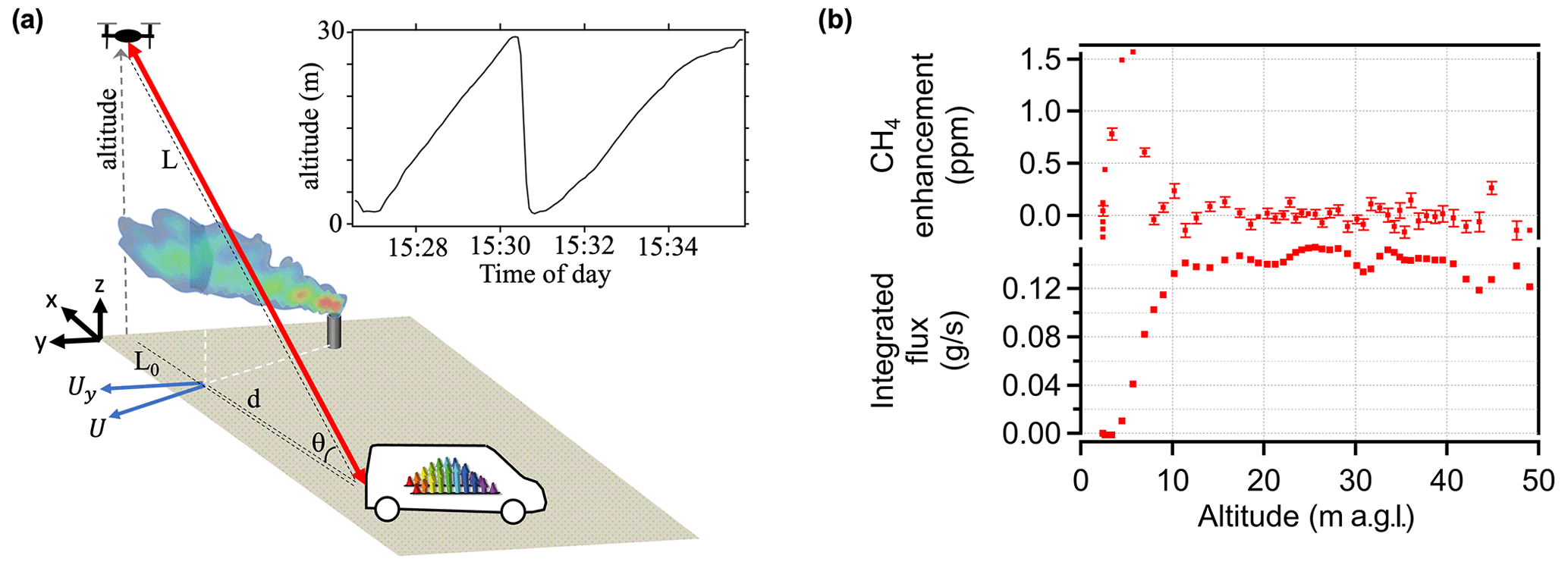
https://amt.copernicus.org/articles/16/5697/2023/amt-16-5697-2023-f04

Figure 4(a) Diagram of the measurement configuration for flux determination from an emission source. The UAV is located a distance L from the DCS system and is scanned vertically with altitude above ground level given by z. The DCS system measures a slant column from the comb system to the UAV and back, as the UAV slowly changes altitude. The plume is transported by the wind vector denoted by U (with the component perpendicular to the measurement plane given by U_y) and intersects the measurement plane a distance d from the comb system. The inset shows an example UAV altitude profile (above ground level) for one flight. (b) Example data from one flight. CH₄ enhancement (top) above background versus UAV altitude. Integrated flux versus (bottom) altitude.

Download

To determine the flux, F, we start by following other mass balance approaches (Alfieri et al., 2010; Karion et al., 2013; Mellqvist et al., 2010). With the geometry of Fig. 4, we assume the x axis is defined by the path from the telescope to the UAV position projected on the ground, and the z axis is vertical. We can then write the flux through a closed surface S as

\begin{matrix} (1) & F = ∯_{S} Δ ρ (x, y, z) U \cdot d A, \end{matrix}

where U is the wind velocity vector, dA is the incremental area of the surface, and $Δ ρ (x, y, z)$ is the gas density above background. If we assume a significant y component to the wind velocity vector, U_y, then the entire plume passes through the x–z plane. Thus, the total flux is found by integrating the enhanced concentration across the x–z plane or

\begin{matrix} (2) & F = \int \int Δ ρ (x, z) U_{y} d x d z . \end{matrix}

However, because the DCS system is measuring a slant column between a fixed point and a moving point – i.e., it measures $Δ \overline{ρ} (r, θ) = \int_{0}^{L} Δ ρ (r, θ) d r$ – we convert Eq. (2) to polar coordinates and restrict the integrals to the plane shown in Fig. 4a ( $0 \leq θ \leq θ_{\max}$ ), assuming that the end position of the UAV in both x and z coordinates lies beyond the plume. Then,

\begin{matrix} (3) & F = \int_{0}^{θ_{\max}} U_{y} \int_{0}^{L} ρ (r, θ) r d r d θ . \end{matrix}

Note the presence of the additional r term in the integral, which means that this integral is not directly what the DCS system measures. To evaluate this, we assume that $ρ (r, θ) = Δ \overline{ρ} (θ) δ (r - d / \cos θ)$ . That is, we assume the plume is localized to intersect the measurement plane at x=d. Then,

\begin{matrix} (4) & F = \int_{0}^{θ_{\max}} U_{y} \int_{0}^{L} Δ \overline{ρ} (θ) δ (r - \frac{d}{\cos θ}) r d r d θ . \end{matrix}

Evaluating the radial integral gives

\begin{matrix} (5) & F = \int_{0}^{θ_{\max}} U_{y} Δ \overline{ρ} (θ) \frac{d}{\cos θ} d θ . \end{matrix}

Converting back to Cartesian coordinates with z=L₀tan θ and assuming that $z ≲ L / 4$ finally gives

\begin{matrix} (6) & F \approx \frac{d}{L_{0}} \int_{0}^{H} U_{y} Δ \overline{ρ} (z) d z, \end{matrix}

where H is the maximum altitude. Equation (6) is derived for the delta-function plume but is valid for other plume shapes where d is defined using the mass-weighted mean. In addition, it assumes that d and L₀ are constant through one flight. We note that the $d / L_{0}$ correction is unnecessary if both the launch and reflector could be moved together, in which case Eq. (2) can be evaluated directly. We can intuitively understand the presence of the $d / L_{0}$ by looking again at a narrow plume intersecting the measurement plane at x=d. The effective altitude range at the plume is $\frac{d}{L_{0}} H$ instead of H; thus, we need to do a change of variable to $z^{'} = \frac{d}{L_{0}} z$ when calculation the altitude integral.

To calculate the flux from a vertical scan, we first interpolate the auxiliary data (UAV location, wind speed and direction, CRDS CH₄) to the DCS data timestamp and filter the DCS data for low a signal-to-noise ratio (for example, if the telescope tracking lost alignment briefly). Then, we determine $Δ {\overline{ρ}}_{g}$ as in Sect. 3.1. Finally, Eq. (6) is numerically integrated to obtain the total flux.

The result of the numerical integration of Eq. (6) versus altitude is shown in Fig. 4b for one flight. For this flight, the CH₄ enhancement profile shows a clear peak between 0 and 10 m a.g.l., which corresponds to a rapid increase in the integrated flux. After 10 m a.g.l., the enhancement has dropped back to background levels and remains near background up to 50 m a.g.l. As expected from this enhancement profile, the integrated flux shows a steady increase from 0 to 10 m a.g.l., after which it remains relatively constant up to 50 m. The variations between 10 and 50 m are driven by measurement noise and provide an estimate of the sensitivity of the flux determination. Note that any offset between the CRDS background and the DCS background would lead to a linear slope during this period from 10 to 50 m, which is not observed in the measurements. From these data, it is also clear that a future system could dispense with the separate CRDS sensor at the van and instead use flat high-AGL measurements or measurements taken upwind of the source by, e.g., combining the scans in Figs. 3 and 4.

3.2.2 Results

Flights were performed across 4 different days (see Appendix A for details of the flights used). Approximately 20 vertical profile flights were conducted; however, on several flights, the wind direction was wrong or shifted early in the flight and caused the plume to miss the measurement path. We note that this information is known in the field from of the meteorological sensors, and the measurement can simply be repeated when the wind has stabilized. In addition, on two flights, the integrated flux was still increasing at the final altitude, indicating that the slant path did not reach the top of the plume, so these flights were discarded from the analysis. In total, 16 flights had sufficient data to determine a flux. Of these, four flights were performed with no release and were evaluated to determine “background” flux. Figure 5 shows a summary of the CH₄ flux determined for these flights.

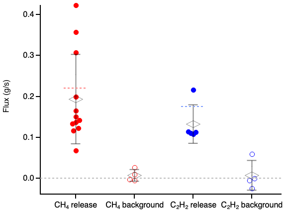
https://amt.copernicus.org/articles/16/5697/2023/amt-16-5697-2023-f05

Figure 5CH₄ and C₂H₂ flux determination for flights with a release and without a release (“background”). A single flight corresponds to a single point for CH₄ and for C₂H₂. For each set, the mean is shown by a diamond and the standard deviation indicated by the vertical lines. The CH₄ release rate was 0.22 g s⁻¹ and the C₂H₂ rate was 0.18 g s⁻¹ as indicated by the dashed horizontal lines.

Download

For the 12 flights with a CH₄ release, the mean flux determined was 0.19 ± 0.11 g s⁻¹ to within 1 standard deviation. The mean agrees within 15 % of the expected flux of 0.22 g s⁻¹, while the standard deviation indicates 56 % uncertainty for a single flight. Of these 12 flights, four flights had a point release and eight flights had a diffuse release, illustrating the capability to measure both types of emissions. No obvious differences were observed for the two release types. For these flights, the distance of the measurement plane downwind from the source varied from ≈ 10 to ≈ 60 m. The four background flights give a mean of 0.008 ± 0.014 g s⁻¹. We estimate the detection limit for CH₄ fluxes as twice the deviation of these background flights, or about 0.03 g s⁻¹. For five flights, C₂H₂ was also released at 0.18 g s⁻¹ with measured flux values of 0.15 ± 0.05 g s⁻¹, again in good agreement with the release rate. The C₂H₂ background flights give a mean of 0.008 ± 0.04 g s⁻¹.

3.2.3 Discussion

The uncertainty in the flux determination is a result of several contributions. First, we note that the accuracy of the methane gas concentration measured by DCS is at the level of ∼ 1 % (Waxman et al., 2017) and is not a significant contribution. The uncertainty arises in the conversion of these measurements to a flux determination via Eq. (6) due to several effects. First, incorrect measurement of the background gas concentrations (for example, due to biases between two CH₄ measurement systems) could lead to an error in $Δ {\overline{ρ}}_{g}$ and a corresponding error in the flux. However, such a bias will result in a linear slope even without a gas flux. From the data in Fig. 4b for altitudes > 10 m, we see no evidence of a linear slope. This is also true in the background flights. Again, this is not surprising given the accuracy of both DCS and the cavity ring-down spectrometer used for the background gas measurements, and we conclude that the evaluation of $Δ {\overline{ρ}}_{g}$ is not a significant source of uncertainty.

Errors in U_y will lead directly to errors in the determined flux. We estimate an upper limit on this error by comparing the two different wind sensors. Their values of U_y averaged over a 10 min flight agree to within ±20 % and typically better. The difference is dominated by uncertainty in the wind speed, rather than the wind direction, given the geometry chosen here where the plume is approximately normal to the measurement plane. (The uncertainty in the wind direction, however, is important below in the determination of d.) The difference in U_y between the anemometers is likely due to true wind differences at the location of the wind sensors. It is possible that a UAV-based wind measurement could reduce this error and improve the flux determination.

There are three sources of uncertainty associated with the value of d in Eq. (1). First, errors in the source location will cause errors in the determination of d. Assuming a random source location uncertainty of Δx, the corresponding uncertainty in d will also be Δx. For the measurements here, the source location was known to better than 1 m, so this uncertainty is negligible. In the case of an initially unknown source location, the approximate location will need to be determined well enough to meet the target accuracy goals based on the measurement configuration. For example, to keep this uncertainty below ±20 %, the source location needs to be known to within ±0.2 d. For the flights here with d≈ 100 m, the location would need to be known within ±20 m. In the case of a uniform diffuse source, the effective weighted center of the source needs to be known to this level. Second, even with a known source location, uncertainty in the wind direction Δϕ will also lead to an uncertainty in d. There are two potential sources of wind direction errors: a static bias during one measurement between the measured wind direction at the sensor and the actual wind direction along the plume trajectory and a temporally varying difference between them. A static bias over one flight will lead to an error given by Δϕ×d_dw, where d_dw is the downwind distance between the source and the measurement plane. Following the geometry here, the downwind distances are < 50 m so that a ±30^∘ wind direction error (estimated from the mean difference between the two anemometers during different flights) corresponds to ±25 m error in d or ±25 % error in the flux for d=100 m. To investigate the impact of the within-flight variability, we recalculated the flux using a time-varying value of d (i.e., mapping d to a slowly varying function d(z) within Eq. 6 using the known values of UAV altitude z as a function of time). For the 10 CH₄ release flights, the change in flux was in all cases < 13 %, with a change in the mean value of 1.4 %, indicating that the impact of temporally varying wind direction differences is minimal. As mentioned above, the static bias could be reduced by measuring the wind direction at the UAV itself. Furthermore, these wind-direction-related errors are minimized with longer measurement paths, which also help to reduce the impact of source location uncertainties. Third and finally, the use of d in Eq. (1) relied on the assumption that the weighted centroid of the plume followed the wind direction from the source to the measurement plane. Plume dynamics are complex and there is some inherent uncertainty in the plume evolution over time. As an estimate of this effect, we assume that the plume centroid is offset on average by at most σ_y from the expected location based on the mean wind direction. The value of σ_y can be taken as the average beam spread in a Gaussian plume model (Seinfeld and Pandis, 2006). For typical daytime conditions with high solar insolation and ∼ 2 m s⁻¹ wind speeds (stability class “A”), σ_y≈15 m, which corresponds to a ±15 % error for d=100 m. The combination of the assumed 20 % uncertainty from the source location, 25 % uncertainty from the wind direction, and 15 % uncertainty from the plume location yields a total ∼ 35 % uncertainty related to d.

Finally, Eq. (2) implicitly assumes the plume location is fixed over the measurement. However, if the vertical position of the plume changes during the measurement, then we have not truly measured the instantaneous flux of Eq. (2). Assuming a flight with vertical velocity, V, and a time-dependent concentration $Δ ρ (x, z, t)$ , the actual measured quantity is

\begin{matrix} (7) & F^{'} = \int \int Δ ρ (x, z, V^{- 1} z) U_{y} d x d z, \end{matrix}

where we ignore the corrections due to the slanted path since they have already been discussed. To estimate the resulting error from vertical translation of the cloud during the measurement, we use a Gaussian plume model,

\begin{matrix} (8) & \begin{aligned} Δ ρ (x, z, t) = & \frac{U_{y} F}{2 π σ_{x} σ_{z}} \exp (- \frac{{(x - x_{0})}^{2}}{2 σ_{x}^{2}}) \\ \exp (- \frac{{(z - z_{0} (t))}^{2}}{2 σ_{z}^{2}}), \end{aligned} \end{matrix}

where the centroid of the two-dimensional plume position is given by (x₀,z₀) with corresponding widths σ_x and σ_y. We write the slowly varying time dependence of the vertical position as $z_{0} (t) = z_{0} + δ z_{0} (t)$ . To lowest order, the vertical position changes due to a small average vertical wind velocity component, U_z, over the roughly 2 min measurement time, giving δz₀(t)=U_zt where $t = V^{- 1} z$ . Substitution of Eq. (8) into Eq. (7) and a Taylor expansion about δz₀ yields the fractional error of the measured quantity compared to the desired flux,

\begin{matrix} (9) & \begin{aligned} |\frac{F^{'}}{F} - 1| = & \frac{U_{z}}{\sqrt{2 π} σ_{z}^{3} V} \int z (z - z_{0}) \\ \exp (- \frac{{(z - z_{0})}^{2}}{2 σ_{z}^{2}}) d z = \frac{U_{z}}{V} . \end{aligned} \end{matrix}

For our flights, we had chosen a relatively slow vertical velocity of V≈0.2 m s⁻¹. Based on measurements from the 3D anemometer, we find a typical vertical wind speed of ∼ 0.05 m s⁻¹, giving an error of ∼ 25 %.

As shown by the background flights, the uncertainty due to DCS measurement noise is expected to contribute ±6 % for a CH₄ flux of 0.22 g s⁻¹. So, when we combine the ±20 % uncertainties associated with the values of U_y, ±35 % uncertainty in d, and ±25 % uncertainty from a time-dependent z₀, we estimate a total estimated uncertainty of ∼ ±50 % in the measured flux values for a single flight, which is in good agreement with the observed uncertainty. Finally, we note that the uncertainties associated with U_y , d, and z₀ described above are statistical (driven by atmospheric variability and plume dynamics) and are thus expected to average down with multiple measurements, as observed here with the low mean bias in the flux determination.

4 Conclusions

We have demonstrated a rapid mass balance method for flux determination using path-integrated slant column measurements between a ground-based measurement system and a UAV located at varying heights above ground. Using a near-infrared dual-comb spectroscopy system, we show flux quantification of CH₄ to within 50 % with a single < 10 min flight and an estimated detection limit of 0.03 g s⁻¹ (2σ), which would enable detection of emissions from 25 head of cattle or from a single pneumatic controller. It is estimated that 90 % of all oil field emissions come from sources that are 10 times larger than this limit (Brandt et al., 2016). We can also simultaneously determine C₂H₂ fluxes with similar performance. This study was designed as a proof of concept for the method. Due to available resources and other logistical considerations, as well as some equipment malfunctions, the measurements were limited in scope. The next step is to do more extensive testing over a range of release conditions, for example, at a facility such as the Methane Emissions Technology Evaluation Center (METEC) (Edie et al., 2020; Riddick et al., 2022).

This new methodology has several potential advantages compared to other flux measurement methods. First, a key advantage is that no atmospheric dispersion model is needed since the flux is determined directly from the data. This also means that multiple spatially separated sources or areal sources can also be measured, although in an area with many sources, care needs to be taken so that the background is appropriate for the sources of interest. A limitation of the specific flight pattern shown is that the source location needs to be approximately known; however, this limitation can be overcome either with a priori information (e.g., if the equipment or facility to be measured is known) or by performing spatial scans first. In addition, modified flight patterns such as flying vertically and then horizontally toward the source could likely overcome this limitation. Second, the methodology is flexible, so it can be used to determine fluxes for any gas that can be measured with open-path dual-comb spectroscopy or other open-path spectroscopy such as active differential optical absorption spectroscopy (Stutz et al., 2016). In particular, CO₂, NH₃, HDO, ethane, formaldehyde (HCHO), CO, and N₂O have all been measured with DCS (Waxman et al., 2017; Ycas et al., 2019; Giorgetta et al., 2021; Herman et al., 2021). By only requiring the lightweight retroreflector to be flown, a small UAV can be used regardless of the gas or gases to be measured.

Combined, these advantages give the capability for rapid, easily deployable, multispecies flux measurements from point or distributed sources. This could be beneficial, for example, to survey emissions from fields, agricultural facilities, wastewater treatment plants, and oil and gas facilities. In addition, with further engineering of mobile DCS, measurements could be conducted from a moving van (similar to the solar occultation flux technique; Mellqvist et al., 2010), allowing for flexible and rapid coverage of a wide area.

Appendix A: Details on the release conditions

Flights were conducted on 7 different days at the Table Mountain facility near Boulder, CO (40.13112, −105.24065). However, only flights from 4 days were able to be used here due to technical issues. On each day, the specific release location was chosen based on the local wind and was sometimes moved if the wind shifted. Flights occurred during daylight, from approximately 10:00–17:00 LT (Mountain Daylight Time). Between 5 and 10 flights were flown per day. Several different flight patterns were flown including the vertical scans used here as well as some flights based on a vertical–radial plume-mapping approach; however, as those flights only contained a few vertical steps, they could not be used for the flux analysis here. Table A1 lists the flights that were used as well as a summary of meteorological conditions for each flight.

Table A1Release information for the processed flights.

Download Print Version | Download XLSX

https://amt.copernicus.org/articles/16/5697/2023/amt-16-5697-2023-f06

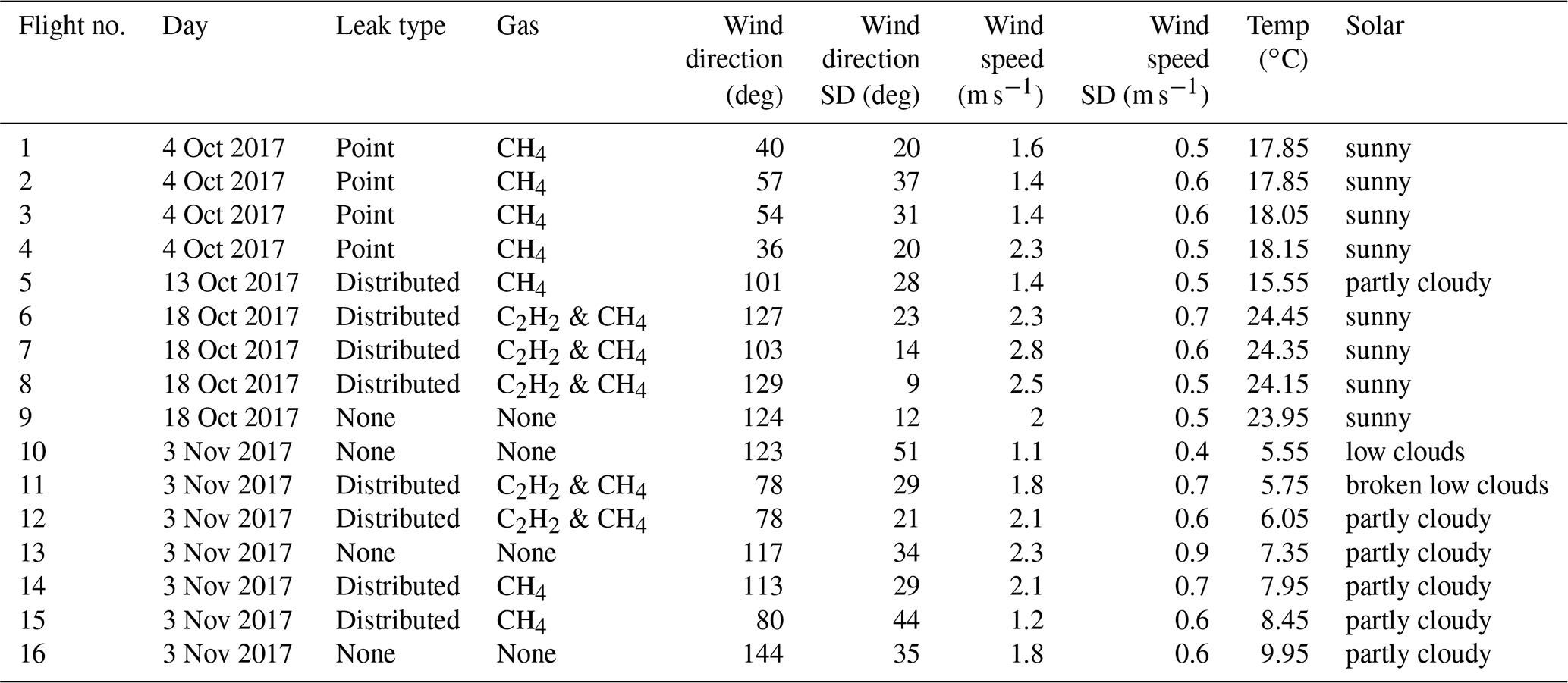
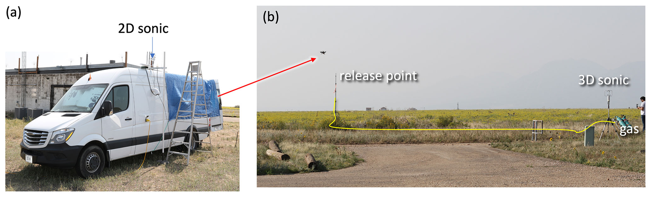
Figure A1Photo of the setup for the controlled releases. (a) The van that housed the dual-comb spectrometer with a 2D sonic anemometer and the weather station (Gill GMX500) mounted to its roof. (b) Standard gas cylinders provided methane and/or acetylene at > 99 % purity. The flow was set by an Alicat MC-20SLPM flow controller with a specified accuracy of ±0.6 %, after which PTFE tubing led to the release point, as discussed in the text. Gas flow for the second gas was set with a ball valve and monitored with a float flowmeter (estimated accuracy ±10 %) A second 3D anemometer (RM Young model 81000 three-axis ultrasonic) provided three-dimensional wind data. The uncertainties in the flow rates were negligible compared to the larger total 50 % uncertainties discussed in the text. As can be seen, the terrain was quite flat with a low cover of grass and brush (< 1 m high) typical of the western United States.

Download

Data availability

Data are available from the authors on request.

Author contributions

KCC and EMW collected and analyzed the data. EH assisted with the field measurements and data collection from the UAV. DH and CC piloted the UAV. KCC, EMW, IC, and NRN wrote and edited the paper.

Competing interests

The contact author has declared that none of the authors has any competing interests.

Disclaimer

Publisher's note: Copernicus Publications remains neutral with regard to jurisdictional claims made in the text, published maps, institutional affiliations, or any other geographical representation in this paper. While Copernicus Publications makes every effort to include appropriate place names, the final responsibility lies with the authors.

Acknowledgements

We thank Michael Cermak for technical assistance, Tim Newberger and Kathryn McCain from NOAA for assistance with the point sensor calibration, and Nathan Malarich, Ryan Cole, and Jerome Genest for helpful discussions on the paper.

Financial support

This research has been funded by the National Institute of Standards and Technology (NIST) and the DARPA Defense Sciences Office.

Review statement

This paper was edited by William R. Simpson and reviewed by two anonymous referees.

References

Alfieri, S., Amato, U., Carfora, M. F., Esposito, M., and Magliulo, V.: Quantifying trace gas emissions from composite landscapes: A mass-budget approach with aircraft measurements, Atmos. Environ., 44, 1866–1876, https://doi.org/10.1016/j.atmosenv.2010.02.026, 2010.

Amediek, A., Ehret, G., Fix, A., Wirth, M., Büdenbender, C., Quatrevalet, M., Kiemle, C., and Gerbig, C.: CHARM-F – a new airborne integrated-path differential-absorption lidar for carbon dioxide and methane observations: measurement performance and quantification of strong point source emissions, Appl. Opt., 56, 5182, https://doi.org/10.1364/AO.56.005182, 2017.

Bai, M., Loh, Z., Griffith, D. W. T., Turner, D., Eckard, R., Edis, R., Denmead, O. T., Bryant, G. W., Paton-Walsh, C., Tonini, M., McGinn, S. M., and Chen, D.: Performance of open-path lasers and Fourier transform infrared spectroscopic systems in agriculture emissions research, Atmos. Meas. Tech., 15, 3593–3610, https://doi.org/10.5194/amt-15-3593-2022, 2022.

Bailey, D. M., Adkins, E. M., and Miller, J. H.: An open-path tunable diode laser absorption spectrometer for detection of carbon dioxide at the Bonanza Creek Long-Term Ecological Research Site near Fairbanks, Alaska, Appl. Phys. B, 123, 245, https://doi.org/10.1007/s00340-017-6814-8, 2017.

Bell, C., Rutherford, J., Brandt, A., Sherwin, E., Vaughn, T., and Zimmerle, D.: Single-blind determination of methane detection limits and quantification accuracy using aircraft-based LiDAR, Elementa Science of the Anthropocene, 10, 00080, https://doi.org/10.1525/elementa.2022.00080, 2022.

Brandt, A. R., Heath, G. A., and Cooley, D.: Methane Leaks from Natural Gas Systems Follow Extreme Distributions, Environ. Sci. Technol., 50, 12512–12520, https://doi.org/10.1021/acs.est.6b04303, 2016.

Coddington, I., Newbury, N., and Swann, W.: Dual-comb spectroscopy, Optica, 3, 414–426, https://doi.org/10.1364/OPTICA.3.000414, 2016.

Conley, S., Faloona, I., Mehrotra, S., Suard, M., Lenschow, D. H., Sweeney, C., Herndon, S., Schwietzke, S., Pétron, G., Pifer, J., Kort, E. A., and Schnell, R.: Application of Gauss's theorem to quantify localized surface emissions from airborne measurements of wind and trace gases, Atmos. Meas. Tech., 10, 3345–3358, https://doi.org/10.5194/amt-10-3345-2017, 2017.

Cossel, K. C., Waxman, E. M., Giorgetta, F. R., Cermak, M., Coddington, I. R., Hesselius, D., Ruben, S., Swann, W. C., Truong, G.-W., Rieker, G. B., and Newbury, N. R.: Open-path dual-comb spectroscopy to an airborne retroreflector, Optica, 4, 724–728, https://doi.org/10.1364/OPTICA.4.000724, 2017.

Cossel, K. C., Waxman, E. M., Baumann, E., Giorgetta, F. R., Coburn, S. C., Alden, C. B., and Washburn, B. R.: 2 – Remote sensing using open-path dual-comb spectroscopy, in: Advances in Spectroscopic Monitoring of the Atmosphere, edited by: Chen, W., Venables, D. S., and Sigrist, M. W., Elsevier, 27–93, https://doi.org/10.1016/B978-0-12-815014-6.00008-7, 2021.

Czepiel, P. M., Mosher, B., Harriss, R. C., Shorter, J. H., McManus, J. B., Kolb, C. E., Allwine, E., and Lamb, B. K.: Landfill methane emissions measured by enclosure and atmospheric tracer methods, J. Geophys. Res.-Atmos., 101, 16711–16719, https://doi.org/10.1029/96JD00864, 1996.

Dobler, J. T., Zaccheo, T. S., Pernini, T. G., Blume, N., Broquet, G., Vogel, F., Ramonet, M., Braun, M., Staufer, J., Ciais, P., and Botos, C.: Demonstration of spatial greenhouse gas mapping using laser absorption spectrometers on local scales, J. Appl. Remote Sens., 11, 014002, https://doi.org/10.1117/1.JRS.11.014002, 2017.

Edie, R., Robertson, A. M., Field, R. A., Soltis, J., Snare, D. A., Zimmerle, D., Bell, C. S., Vaughn, T. L., and Murphy, S. M.: Constraining the accuracy of flux estimates using OTM 33A, Atmos. Meas. Tech., 13, 341–353, https://doi.org/10.5194/amt-13-341-2020, 2020.

Gålfalk, M., Nilsson Påledal, S., and Bastviken, D.: Sensitive Drone Mapping of Methane Emissions without the Need for Supplementary Ground-Based Measurements, ACS Earth Space Chem., 5, 2668–2676, https://doi.org/10.1021/acsearthspacechem.1c00106, 2021.

Giorgetta, F. R., Peischl, J., Herman, D. I., Ycas, G., Coddington, I., Newbury, N. R., and Cossel, K. C.: Open-Path Dual-Comb Spectroscopy for Multispecies Trace Gas Detection in the 4.5–5 µm Spectral Region, Laser Photonics Rev., 15, 2000583, https://doi.org/10.1002/lpor.202000583, 2021.

Golston, L. M., Aubut, N. F., Frish, M. B., Yang, S., Talbot, R. W., Gretencord, C., McSpiritt, J., and Zondlo, M. A.: Natural Gas Fugitive Leak Detection Using an Unmanned Aerial Vehicle: Localization and Quantification of Emission Rate, Atmosphere, 9, 333, https://doi.org/10.3390/atmos9090333, 2018.

Herman, D. I., Weerasekara, C., Hutcherson, L. C., Giorgetta, F. R., Cossel, K. C., Waxman, E. M., Colacion, G. M., Newbury, N. R., Welch, S. M., DePaola, B. D., Coddington, I., Santos, E. A., and Washburn, B. R.: Precise multispecies agricultural gas flux determined using broadband open-path dual-comb spectroscopy, Sci. Adv., 7, eabe9765, https://doi.org/10.1126/sciadv.abe9765, 2021.

Johnson, M. R., Tyner, D. R., and Szekeres, A. J.: Blinded evaluation of airborne methane source detection using Bridger Photonics LiDAR, Remote Sens. Environ., 259, 112418, https://doi.org/10.1016/j.rse.2021.112418, 2021.

Karion, A., Sweeney, C., Pétron, G., Frost, G., Michael Hardesty, R., Kofler, J., Miller, B. R., Newberger, T., Wolter, S., Banta, R., Brewer, A., Dlugokencky, E., Lang, P., Montzka, S. A., Schnell, R., Tans, P., Trainer, M., Zamora, R., and Conley, S.: Methane emissions estimate from airborne measurements over a western United States natural gas field, Geophys. Res. Lett., 40, 4393–4397, https://doi.org/10.1002/grl.50811, 2013.

Kille, N., Baidar, S., Handley, P., Ortega, I., Sinreich, R., Cooper, O. R., Hase, F., Hannigan, J. W., Pfister, G., and Volkamer, R.: The CU mobile Solar Occultation Flux instrument: structure functions and emission rates of NH₃, NO₂ and C₂H₆, Atmos. Meas. Tech., 10, 373–392, https://doi.org/10.5194/amt-10-373-2017, 2017.

Kunkel, W., Thorpe, M., Carre-Burritt, A., Aivazian, G., Snow, N., Harris, J., Mueller, T., and Roos, P.: Extension of Methane Emission Rate Distribution for Permian Basin Oil and Gas Production Infrastructure by Aerial LiDAR, Environ. Sci. Technol., 57, 12234–12241, 2023.

Mellqvist, J., Samuelsson, J., Johansson, J., Rivera, C., Lefer, B., Alvarez, S., and Jolly, J.: Measurements of industrial emissions of alkenes in Texas using the solar occultation flux method, J. Geophys. Res., 115, D00F17, https://doi.org/10.1029/2008JD011682, 2010.

Mønster, J. G., Samuelsson, J., Kjeldsen, P., Rella, C. W., and Scheutz, C.: Quantifying methane emission from fugitive sources by combining tracer release and downwind measurements – A sensitivity analysis based on multiple field surveys, Waste Manage., 34, 1416–1428, https://doi.org/10.1016/j.wasman.2014.03.025, 2014.

Picqué, N. and Hänsch, T. W.: Frequency comb spectroscopy, Nat. Photonics, 13, 146–157, https://doi.org/10.1038/s41566-018-0347-5, 2019.

Plant, G., Nikodem, M., Mulhall, P., Varner, R. K., Sonnenfroh, D., and Wysocki, G.: Field Test of a Remote Multi-Path CLaDS Methane Sensor, Sensors, 15, 21315–21326, https://doi.org/10.3390/s150921315, 2015.

Ravikumar, A. P., Sreedhara, S., Wang, J., Englander, J., Roda-Stuart, D., Bell, C., Zimmerle, D., Lyon, D., Mogstad, I., Ratner, B., and Brandt, A. R.: Single-blind inter-comparison of methane detection technologies – results from the Stanford/EDF Mobile Monitoring Challenge, Elem. Sci. Anth., 7, 37, https://doi.org/10.1525/elementa.373, 2019.

Reuter, M., Bovensmann, H., Buchwitz, M., Borchardt, J., Krautwurst, S., Gerilowski, K., Lindauer, M., Kubistin, D., and Burrows, J. P.: Development of a small unmanned aircraft system to derive CO₂ emissions of anthropogenic point sources, Atmos. Meas. Tech., 14, 153–172, https://doi.org/10.5194/amt-14-153-2021, 2021.

Riddick, S. N., Ancona, R., Mbua, M., Bell, C. S., Duggan, A., Vaughn, T. L., Bennett, K., and Zimmerle, D. J.: A quantitative comparison of methods used to measure smaller methane emissions typically observed from superannuated oil and gas infrastructure, Atmos. Meas. Tech., 15, 6285–6296, https://doi.org/10.5194/amt-15-6285-2022, 2022.

Roscioli, J. R., Yacovitch, T. I., Floerchinger, C., Mitchell, A. L., Tkacik, D. S., Subramanian, R., Martinez, D. M., Vaughn, T. L., Williams, L., Zimmerle, D., Robinson, A. L., Herndon, S. C., and Marchese, A. J.: Measurements of methane emissions from natural gas gathering facilities and processing plants: measurement methods, Atmos. Meas. Tech., 8, 2017–2035, https://doi.org/10.5194/amt-8-2017-2015, 2015.

Rothman, L. S., Gordon, I. E., Barbe, A., Benner, D. C., Bernath, P. E., Birk, M., Boudon, V., Brown, L. R., Campargue, A., Champion, J. P., Chance, K., Coudert, L. H., Dana, V., Devi, V. M., Fally, S., Flaud, J. M., Gamache, R. R., Goldman, A., Jacquemart, D., Kleiner, I., Lacome, N., Lafferty, W. J., Mandin, J. Y., Massie, S. T., Mikhailenko, S. N., Miller, C. E., Moazzen-Ahmadi, N., Naumenko, O. V., Nikitin, A. V., Orphal, J., Perevalov, V. I., Perrin, A., Predoi-Cross, A., Rinsland, C. P., Rotger, M., Simeckova, M., Smith, M. A. H., Sung, K., Tashkun, S. A., Tennyson, J., Toth, R. A., Vandaele, A. C., and Vander Auwera, J.: The HITRAN 2008 molecular spectroscopic database, J. Quant. Spectrosc. Ra., 110, 533–572, https://doi.org/10.1016/j.jqsrt.2009.02.013, 2009.

Seinfeld, J. H. and Pandis, S. N.: Atmospheric Chemistry and Physics: From Air Pollution to Climate Change, Wiley, 3rd edn., 1120 pp., ISBN 9781118947401, 2016.

Soskind, M. G., Li, N. P., Moore, D. P., Chen, Y., Wendt, L. P., McSpiritt, J., Zondlo, M. A., and Wysocki, G.: Stationary and drone-assisted methane plume localization with dispersion spectroscopy, Remote Sens. Environ., 289, 113513, https://doi.org/10.1016/j.rse.2023.113513, 2023.

Stutz, J., Hurlock, S. C., Colosimo, S. F., Tsai, C., Cheung, R., Festa, J., Pikelnaya, O., Alvarez, S., Flynn, J. H., Erickson, M. H., and Olaguer, E. P.: A novel dual-LED based long-path DOAS instrument for the measurement of aromatic hydrocarbons, Atmos. Environ., 147, 121–132, https://doi.org/10.1016/j.atmosenv.2016.09.054, 2016.

Truong, G.-W., Waxman, E. M., Cossel, K. C., Baumann, E., Klose, A., Giorgetta, F. R., Swann, W. C., Newbury, N. R., and Coddington, I.: Accurate frequency referencing for fieldable dual-comb spectroscopy, Opt. Express, 24, 30495–30504, https://doi.org/10.1364/OE.24.030495, 2016.

Vaughn, T. L., Bell, C. S., Yacovitch, T. I., Roscioli, J. R., Herndon, S. C., Conley, S., Schwietzke, S., Heath, G. A., Pétron, G., and Zimmerle, D.: Comparing facility-level methane emission rate estimates at natural gas gathering and boosting stations, Elem. Sci. Anth., 5, 71, https://doi.org/10.1525/elementa.257, 2017.

Waxman, E. M., Cossel, K. C., Truong, G.-W., Giorgetta, F. R., Swann, W. C., Coburn, S., Wright, R. J., Rieker, G. B., Coddington, I., and Newbury, N. R.: Intercomparison of open-path trace gas measurements with two dual-frequency-comb spectrometers, Atmos. Meas. Tech., 10, 3295–3311, https://doi.org/10.5194/amt-10-3295-2017, 2017.

White, W. H., Anderson, J. A., Blumenthal, D. L., Husar, R. B., Gillani, N. V., Husar, J. D., and Wilson, W. E.: Formation and transport of secondary air pollutants: ozone and aerosols in the St. Louis urban plume, Science, 194, 187–189, https://doi.org/10.1126/science.959846, 1976.

Ycas, G., Giorgetta, F. R., Cossel, K. C., Waxman, E. M., Baumann, E., Newbury, N. R., and Coddington, I.: Mid-infrared dual-comb spectroscopy of volatile organic compounds across long open-air paths, Optica, 6, 165–168, https://doi.org/10.1364/OPTICA.6.000165, 2019.

Zhang, E. J., Teng, C. C., van Kessel, T. G., Klein, L., Muralidhar, R., Wysocki, G., and Green, W. M. J.: Field Deployment of a Portable Optical Spectrometer for Methane Fugitive Emissions Monitoring on Oil and Gas Well Pads, Sensors, 19, 2707, https://doi.org/10.3390/s19122707, 2019.

Zondlo, M. A.: 6 – Unmanned aerial systems for trace gases, in: Advances in Spectroscopic Monitoring of the Atmosphere, edited by: Chen, W., Venables, D. S., and Sigrist, M. W., Elsevier, 321–343, https://doi.org/10.1016/B978-0-12-815014-6.00007-5, 2021.

Articles

Executive editor

As the Editor states does this manuscript describe application of long-path absorption spectroscopy to detection of gas leak plumes. The technique uses an unmanned aerial vehicle (UAV) carrying a retroreflector as the endpoint of the absorption path, which allows for rapid discovery of plume location and quantification of plume cross section for emissions rate determination. The technique works at a safe standoff distance and through the use of the UAV doesn't need two fixed end locations. It would be of interest to many seeking to find and quantify gas leaks, which is important for safety and minimizing greenhouse gas and reactive gas emissions.

Short summary

Measurements of the emission rate of a gas or gases from point and area sources are important in a range of monitoring applications. We demonstrate a method for rapid quantification of the emission rate of multiple gases using a spatially scannable open-path sensor. The open-path spectrometer measures the total column density of gases between the spectrometer and a retroreflector mounted on an uncrewed aerial vehicle (UAV). By scanning the UAV altitude, we can determine the total gas emissions.