Methane retrievals from airborne HySpex observations in the shortwave infrared

Hochstaffl, Philipp; Schreier, Franz; Köhler, Claas Henning; Baumgartner, Andreas; Cerra, Daniele

doi:https://doi.org/10.5194/amt-16-4195-2023

Articles | Volume 16, issue 18

https://doi.org/10.5194/amt-16-4195-2023

Special issue:

CoMet: a mission to improve our understanding and to better...

https://doi.org/10.5194/amt-16-4195-2023

Articles | Volume 16, issue 18

Research article

19 Sep 2023

Research article |

| 19 Sep 2023

Methane retrievals from airborne HySpex observations in the shortwave infrared

Philipp Hochstaffl, Franz Schreier, Claas Henning Köhler, Andreas Baumgartner, and Daniele Cerra

Abstract

Monitoring anthropogenic emissions is a crucial aspect in understanding the methane budget. Moreover, a reduction of methane emissions could help to mitigate global warming on a short timescale. This study compares various retrieval schemes for estimating localized methane enhancements around ventilation shafts in the Upper Silesian Coal Basin in Poland using nadir observations in the shortwave infrared acquired from the airborne imaging spectrometer HySpex. Linear and nonlinear solvers are examined and compared, with special emphasis put on strategies that tackle degeneracies between the surface reflectivity and broad-band molecular absorption features – a challenge arising from the instrument's low spectral resolution. Results reveal that the generalized nonlinear least squares fit, employed within the Beer InfraRed Retrieval Algorithm (BIRRA), can measure enhanced methane levels with notable accuracy and precision. This is accomplished by allowing the scene's background covariance structure to account for surface reflectivity statistics. Linear estimators such as matched filter (MF) and singular value decomposition (SVD) are able to detect and, under favorable conditions, quantify enhanced levels of methane quickly. Using k-means clustering as a preprocessing step can further enhance the performance of the two linear solvers. The linearized BIRRA fit (LLS) underestimates methane but agrees on the enhancement pattern. The non-quantitative spectral signature detection (SSD) method does not require any forward modeling and can be useful in the detection of relevant scenes. In conclusion, the BIRRA code, originally designed for the retrieval of atmospheric constituents from spaceborne high-resolution spectra, turned out to be applicable to hyperspectral airborne imaging data for the quantification of methane plumes from point-like sources. Moreover, it is able to outperform well-established linear schemes such as the MF or SVD at the expense of high(er) computing time.

Download & links

How to cite

How to cite.

Dates

Received: 29 Sep 2022 – Discussion started: 24 Nov 2022 – Revised: 06 Jul 2023 – Accepted: 20 Jul 2023 – Published: 19 Sep 2023

1 Introduction

Methane (CH₄) is the second most important anthropogenic greenhouse gas next to carbon dioxide (CO₂), according to the IPCC (Intergovernmental Panel on Climate Change; Masson-Delmotte et al., 2021) report. Due to its comparatively short lifetime of approximately 9 years, a reduction of methane emissions could help to mitigate global warming on a relatively short timescale. Despite improvements in monitoring regional and global CH₄ emissions in recent years, the IPCC report points out that fundamental uncertainties pertaining to the methane budget remain (Intergovernmental Panel on Climate Change, 2014).

The vast majority of anthropogenic CH₄ emissions are caused by small-scale processes such as agriculture (enteric fermentation and manure), waste management (landfills), and fossil fuel exploitation, where the last is responsible for 20 %–30 % of all anthropogenic CH₄ emissions. Consequently, there is a need for continuous long-term methane observations on local to global scales in order to foster understanding on the global methane cycle, devise future reduction measures, and monitor their effectiveness. The monitoring of anthropogenic emissions of CH₄ and CO₂ is also part of the United Nations Framework Convention on Climate (2015), as nationally determined contributions should be assessed via global stock takes on a 5-year basis from 2023 (Article 13 and 14 of the Paris Agreement).

Satellite observations are typically used for continuous and global long-term monitoring of atmospheric composition, but also ground-based networks such as the Global Atmosphere Watch (GAW) Programme of the World Meteorological Organization (WMO) or the European Integrated Carbon Observation System (ICOS) are crucial assets. Spaceborne spectrometers measuring shortwave infrared (SWIR) solar radiation reflected at the Earth's surface are especially well suited to observe atmospheric CH₄ in the lower atmosphere by measuring its absorption around 1.6 and 2.3 µm. In contrast, the thermal infrared is less sensitive to variations in CH₄ concentration close to the surface, while mid-infrared sensors often have lower spatial resolution making them less favorable for emission monitoring (Richter, 2010).

Operational CH₄ products from contemporary atmospheric composition missions such as TROPOMI (TROPOspheric Monitoring Instrument; Veefkind et al., 2012) and GOSAT/GOSAT-2 (Greenhouse gases Observing SATellite; Kuze et al., 2009, 2016) measure trace gas concentrations with very high accuracy. Nevertheless, they are not optimally suited to measure emissions of point sources. This limitation is due to their focus on rapid global coverage, which entails a comparatively coarse spatial resolution of several square kilometers per pixel. Since the emission of a single point source inside a pixel is averaged over the entire resolution cell, even large sources rarely elevate the mean CH₄ concentration within one pixel by more than 1 % compared to the undisturbed background (Lauvaux et al., 2022). A way to increase the contrast of enhancements is to operate typical atmospheric remote sensing spectrometers at lower altitudes (e.g., on aircraft), thus increasing the spatial resolution while leaving the overall optical design untouched. This strategy is followed by instruments such as MAMAP/MAMAP-2D (Gerilowski et al., 2011) or GHOST (Humpage et al., 2018), which are well suited for the calibration and validation of their spaceborne counterparts.

Another way to increase the sensitivity towards smaller sources is to increase the instrument's spatial resolution. This in turn necessitates a trade-off in spectral resolution because the loss of photons caused by the smaller ground pixels reduces the signal-to-noise ratio (SNR) of the image, which has to be compensated for by broadening the width of the spectral channels. Imaging spectrometers for land surface remote sensing (often referred to as hyperspectral cameras) are typical examples of instruments optimized for spatial resolution this way. Their technology matured over the last 30 years, and a variety of airborne instruments and several spaceborne versions are either in orbit (Cogliati et al., 2021, PRISMA), (Guanter et al., 2015; Chabrillat et al., 2020, ENMAP) or going to be launched in the future (Rast et al., 2021, CHIME). Yet other sensors dedicated for the detection of methane or carbon dioxide, e.g., GHGSat (Jervis et al., 2021), CO2Image (Hochstaffl et al., 2023), or MethaneSat, have slightly higher spectral resolution than their hyperspectral counterparts but still offer a much higher spatial resolution than classical atmospheric composition missions.

Thorpe et al. (2013) were the first to demonstrate that localized CH₄ emissions over land can be detected from hyperspectral cameras with the Airborne Visible/Infrared Imaging Spectrometer (Green et al., 1998, AVIRIS) and that a limited quantitative analysis is possible (Thorpe et al., 2014). Similar studies were repeated with airborne instruments (AVIRIS-NG, Frankenberg et al., 2016; Duren et al., 2019; Borchardt et al., 2021; HySpex, Nesme et al., 2020) and spaceborne instruments (Thompson et al., 2016; Guanter et al., 2021). Varon et al. (2019) and Jervis et al. (2021) demonstrated that CH₄ sources can even be detected with the Multispectral Instrument (MSI) aboard the Sentinel-2 satellites, but these measurements are restricted to “favorable conditions” (i.e., strong sources and high surface albedo).

One of the core challenges when retrieving methane from measurements with high spatial (⪅100 m) and moderate spectral resolution (⪆1 nm) is the separation of spectral variations caused by molecular absorption and surface reflectivity (Ayasse et al., 2018). Classical methods for trace gas retrievals from high-spectral resolution instruments such as RemoTeC (Lorente et al., 2021), Weighting Function Modified Differential Optical Absorption Spectroscopy (Buchwitz et al., 2005, WFM-DOAS), or the Beer InfraRed Retrieval Algorithm (Gimeno García et al., 2011, BIRRA) exploit the high-frequency characteristics of gaseous absorption and attribute the smooth varying part to the surface albedo (and scattering). Instruments with coarse spectral resolution, however, are unable to sufficiently resolve those molecular signatures which causes ambiguities that often lead to surface-type-related biases in the classical retrieval schemes (e.g., Borchardt et al., 2021, Sect. 3.3, or Thorpe et al., 2014, Sect. 9.2). Alternative more data-driven retrieval schemes such as matched filter (MF) or singular value decomposition (SVD) employ methods from linear algebra and statistics that deal with spectral correlations and often yield results of sufficient accuracy (Thorpe et al., 2013, 2014; Thompson et al., 2015).

This study aims to compare concentration enhancements from different retrieval methods using measurements of the German Aerospace Center's (DLR) HySpex sensor system. The objective is to evaluate the retrievals' performance in terms of accuracy, precision, and speed and show advantages and drawbacks for each method. Another goal is to assess the latest BIRRA updates and its applicability to moderately resolved spectra from airborne sensors. Therefore, the paper is structured as follows.

First, the experimental setup is briefly described, followed by a quick review of atmospheric radiation and an introduction to the various BIRRA setups examined in this study. Afterwards, other simpler but faster retrieval schemes employed in this work are briefly discussed. The result section presents the CH₄ retrievals from HySpex observations over the Pniówek V ventilation shafts and compares the inferred concentrations and errors from the different methods. In the last section, results are summarized and put into perspective.

2 Methodology

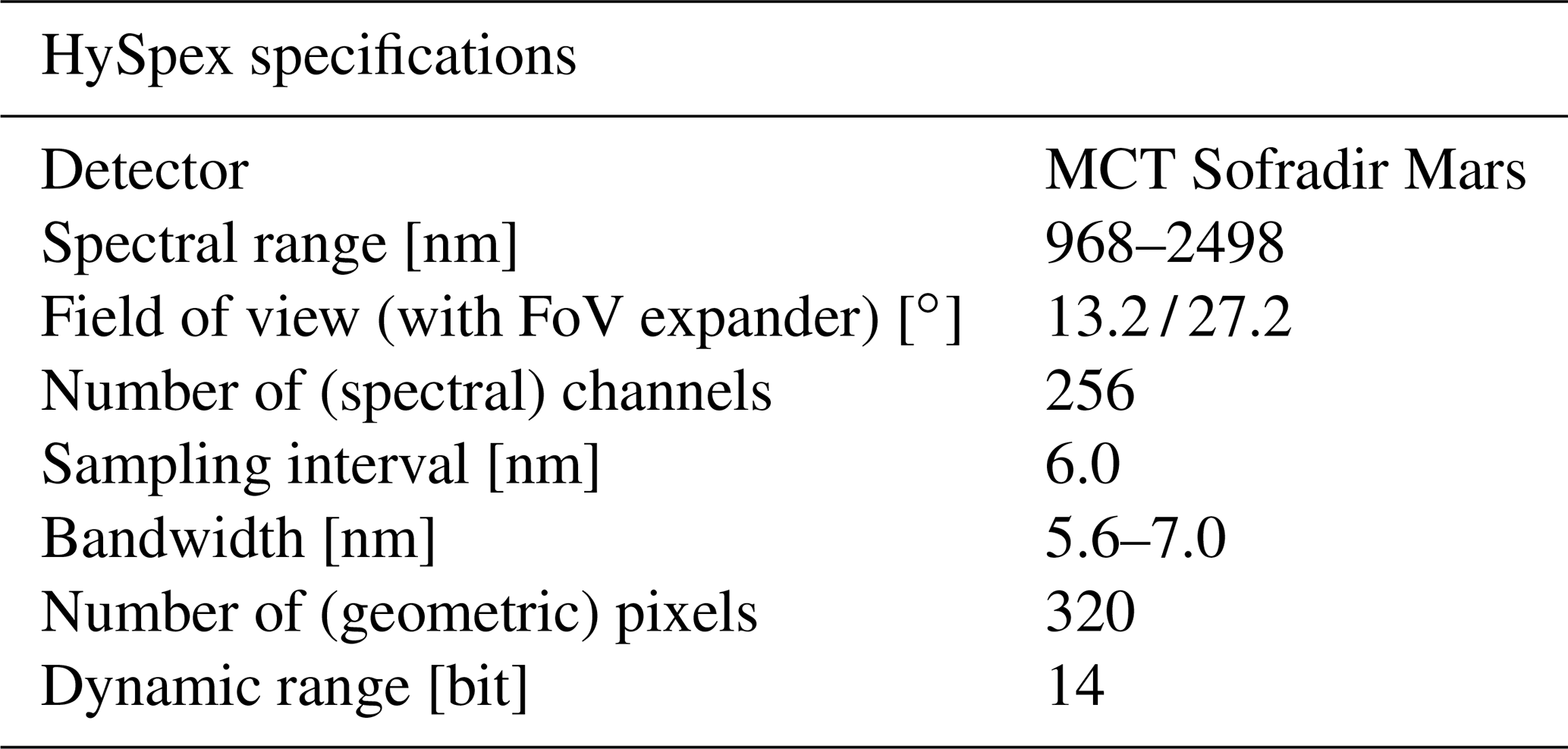
Both linear and nonlinear methane retrieval schemes are examined. While the former are very fast but often lack sufficient accuracy, nonlinear iterative solvers require more computing power and time to come up with a best estimate. The study utilizes measurements collected by the DLR airborne HySpex sensor system (see Table 1) within the scope of the COMET (Carbon Dioxide and Methane) campaign on 7 June 2018 which focused on the detection and characterization of CO₂ and CH₄ sources in the Upper Silesian Coal Basin (USCB) in southern Poland.

Table 1Summary of some important HySpex properties. The sensor is described in detail in Köhler (2016) and references therein.

Download Print Version | Download XLSX

To compare the performance of various retrieval methods, we limit our analysis to the two flight lines shown in Fig. 1, namely flight line 9 (called scene 09) and flight line 11 (called scene 11). The weather during the survey was well suited for remote sensing measurements. Apart from very few occasional patches of thin cirrus clouds, no further low- or mid-level clouds were near. Actual wind data for the USCB area are presented in Luther et al. (2022, Figs. 4 and 6).

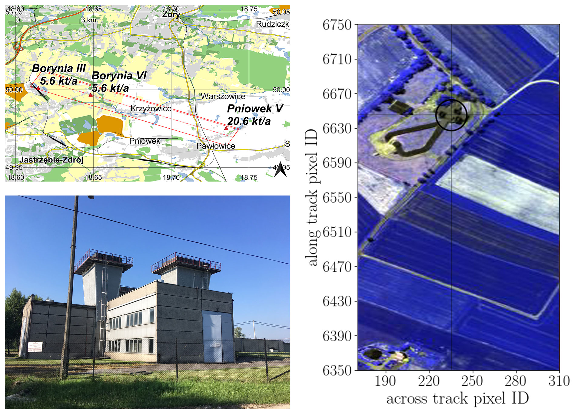
https://amt.copernicus.org/articles/16/4195/2023/amt-16-4195-2023-f01

Figure 1(Left, top) Flight line 9 (dashed red line) was obtained around 09:55 UTC, while flight line 11 (solid red line) was acquired around 10:10 UTC (© OpenStreetMap contributors, 2022; distributed under the Open Data Commons Open Database License (ODbL) v1.0). The aircraft flew at an altitude of approximately ≈1200 and ≈2600 m above ground level, respectively, while heading eastward at 115^∘. (Left, bottom) Photograph of the ventilation shafts from the Pniówek V site. Photo credit: Leon Scheidweiler (Heidelberg University). (Right) False-color image from the SWIR-320m-e camera around the three Pniówek V shafts in scene 09.

Figure 2 (top) displays an ensemble of along-track-averaged HySpex observations. The spectral coverage of the HySpex SWIR-320m-e camera ranges from 967–2496 nm, with the exact number depending on the across-track detector ( $\approx \pm 1$ cm⁻¹). The full width at half maximum (FWHM) of the SWIR-320m-e camera in the 1500–2500 nm (4000–6500 cm⁻¹) region ranges from 6.0–9.5 nm and is provided with the level 1b data for a sampling distance of 1.2 nm. The figure shows that the radiative intensity in the interval around 1.6 µm (≈6000 cm⁻¹) is significantly larger than the one around 2.3 µm (≈4300 cm⁻¹) mostly due to H₂O absorption (see Fig. 3). A possible bad pixel (number 104) is shown in the right plot around 1.65 nm (a descending cyan line). Also the surface reflectivity, depicted in Fig. 1, causes spectral variations in the observed radiance.

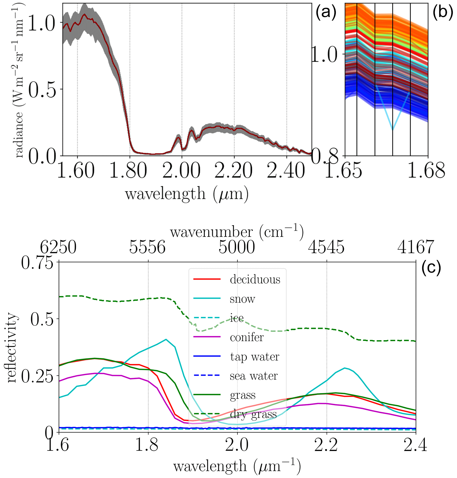
https://amt.copernicus.org/articles/16/4195/2023/amt-16-4195-2023-f02

Figure 2(a) HySpex average spectrum with the span (minimum to maximum) depicted in gray for measurements across the 320 across-track detectors for scene 09. (b) A bunch of individual spectra around 1.67 µm with the black lines indicating the pixel positions and sampling distance. The radiance values of pixel 104 (cyan) at ≈1.677 µm (5960 cm⁻¹), which is relevant for the CH₄ retrieval, appear to be problematic. (c) Reference reflectances for different surface types (measured at the Johns Hopkins University, Baldridge et al., 2009; Meerdink et al., 2019).

Download

https://amt.copernicus.org/articles/16/4195/2023/amt-16-4195-2023-f03

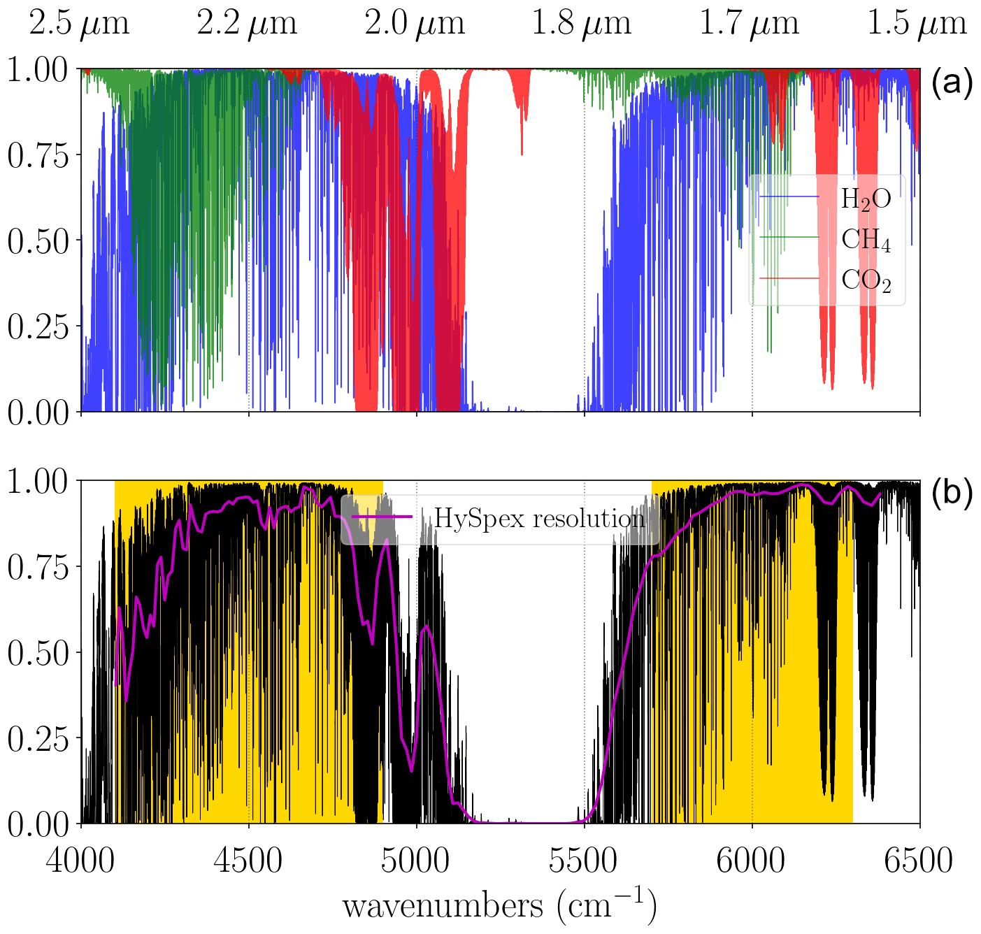
Figure 3(a) Monochromatic transmissions of CH₄, CO₂, and H₂O for the SWIR spectral range and a nadir-looking observer at 1.5 km at a solar zenith angle (SZA) of 30^∘. (b) Total monochromatic transmission (black) vs. degraded to HySpex resolution (magenta). The spectral intervals used for the CH₄ fit are indicated by the yellow background.

Download

2.1 Radiative transfer

In the SWIR spectral range the radiative transfer through the atmosphere under clear-sky conditions (cloud and scattering free) is well described by Beer's law (Zdunkowski et al., 2007) with the monochromatic transmission in wavenumbers ν given by

\begin{matrix} (1) & \begin{aligned} T_{m} (ν, s) & = \exp (- \sum_{m} τ_{m} (ν, s)) \\ = \exp (- \int_{path} d s \sum_{m} n_{m} (s) k_{m} (ν, p (s), T (s))) . \end{aligned} \end{matrix}

The model assumes a pure gas atmosphere of molecules m, i.e., CH₄, CO₂, and H₂O. Optical depth τ_m is calculated by the path integral along s over the molecular number densities n_m and the pressure p and temperature T dependent absorption cross section k_m. The study utilizes the 2020 spectroscopic line data from GEISA (Gestion et Etude des Informations Spectroscopiques Atmosphériques; Delahaye et al., 2021) for molecular absorption calculations.

The decision to exclude aerosol modeling for HySpex observations was encouraged by findings from Borchardt et al. (2021), who concluded that different aerosol scenarios in the SWIR do not induce errors greater than 0.2 %. Moreover, since the spectra were observed at low flight altitudes on a rather clear day, retrieval errors induced by aerosol scattering should be negligible in our scenario as well (also see Fig. 3 and Thorpe et al., 2013; Thompson et al., 2015).

In Fig. 3, the top panel shows the individual components of the monochromatic total transmission for the US Standard Atmosphere, including methane's first overtone of the fundamental vibrational transition 2ν₃ (with its P and R branches) around 6000 cm⁻¹ (1560–1660 nm, tetradecad band), as well as additional strong absorption lines ranging from 4200–4600 cm⁻¹ (2090–2290 nm, octad). The bottom panel illustrates how the observer's coarse spectral resolution smooths the total monochromatic transmission (shown in black). There are 67 and 28 HySpex detectors used by the retrievals (see Fig. 3) within the range of 4100–4900 cm⁻¹ (4K) and 5700–6300 cm⁻¹ (6K), respectively.

2.2 Model atmosphere setup

The model atmosphere's vertical extent ranges from 0–80 km with 39 levels in total. The atmosphere is composed of pure gaseous layers. The highest vertical resolution is found in those layers below z_pl=2 km where the enhancement is expected to take place. The CH₄ optical depth is divided in two components, i.e., a climatological background τ_bg and a low-level (Gaussian) plume τ. The vertical profile of the initial guess plume is not crucial since nadir spectra in the SWIR do not contain sufficient information on the vertical distribution of trace gases (see Hochstaffl et al., 2020, Fig. 7).

The CH₄ and CO₂ initial guess background profiles are modeled according to the Air Force Geophysics Laboratory (AFGL) but adjusted to current concentrations in the atmosphere (1875 ppb and 400 ppm, respectively; cf. Sect. 2.3.2). H₂O and temperature and pressure are taken from reanalysis data provided by the National Centers for Environmental Prediction (Kalnay et al., 1996, NCEP).

2.3 Beer InfraRed Retrieval Algorithm (BIRRA)

The classical BIRRA level 2 processor, developed at DLR, uses the Generic Atmospheric Radiation Line-by-line Infrared Code (Schreier et al., 2014, GARLIC) as a forward model and a separate (SLS) or nonlinear least squares solver (NLS) for trace gas retrieval in the SWIR spectral region. It has been successfully applied to SCIAMACHY (SCanning Imaging Absorption spectroMeter for Atmospheric CHartographY; Gimeno García et al., 2011; Hochstaffl et al., 2018) and TROPOMI (TROPOspheric Monitoring Instrument, Hochstaffl et al., 2020) observations. In this study, however, the new Python version of BIRRA which is based on Py4CAtS (Python for Computational Atmospheric Spectroscopy, Schreier et al., 2019), a Python reimplementation of the validated Fortran code GARLIC (Schreier et al., 2013) is used.

The mathematical forward model Φ(x,ν) describes the measured intensity spectrum I(ν) for a nadir-looking observer according to

\begin{matrix} (2) & Φ (x, ν) = \frac{r (ν)}{π} \cos (θ) I_{sun} (ν) T_{m}^{↓} (ν) T_{m}^{↑} (ν) \otimes S (ν, γ (ν)), \end{matrix}

where r refers to the surface reflectivity and θ represents the solar zenith angle. The terms $T_{m}^{↓}$ and $T_{m}^{↑}$ denote the total transmission between the Sun and the reflection point (e.g., the Earth) and between the reflection point and the observer, respectively (see Eq. 1).

The transmission is described by

\begin{matrix} (3) & T_{m} (ν, s) = \exp (- \sum_{m} α_{m} τ_{m} (ν)), \end{matrix}

where the molecular scaling factors α_m adjust initial guess profiles. The simple scaling approach recognizes the significantly under-determined vertical profile information in the observed spectrum and enables an unconstrained least squares fit. All unknown (to be estimated) parameters are collected in the state vector x, which includes α_m and the polynomial coefficients for the surface reflectivity r_j (with j∈ℕ₀) (Gimeno García et al., 2011, Fig. 1). Finally, the instrument’s spectral response function (ISRF) is described by S. Its parameters such as the half width γ or a spectral shift can (optionally) be part of the state vector (also see Thorpe et al., 2014, Sect. 5.2).

2.3.1 Nonlinear solvers

This study examines various nonlinear retrieval schemes that are implemented in the BIRRA level 2 processor and are briefly introduced below. Nonlinear least squares methods are iterative and require calculating derivatives for each of the nonlinear state vector elements, represented by a Jacobian matrix J.

Nonlinear least squares (NLS) and separable least squares (SLS)

The nonlinear least squares fit minimizes the residual norm ( $‖ \cdot ‖$ represents the 2-norm) for given measurements y when the model function Φ is nonlinear in one or more parameters of x according to

\begin{matrix} (4) & min_{x} {∥y - Φ (x)∥}^{2} . \end{matrix}

The SLS splits (separates) the state vector x into nonlinear and linear parameters $x = (η, ζ)$ , where the elements in ζ enter the forward model Φ linearly (see Sect. 2.4.1). The minimization problem is hence given by

\begin{matrix} (5) & min_{η, ζ} {∥y - Φ (η) ζ (η)∥}^{2} . \end{matrix}

This setup is also known as the variable projection (VarPro, Golub and Pereyra, 2003) method, where η is independent of ζ in the matrix product Φ(η)ζ(η) (for details see Bärligea et al., 2023). The parameters in η can hence be fitted in the usual way by means of Gauss–Newton or Levenberg–Marquardt algorithms (see Hansen et al., 2013).

Generalized least squares (GLS)

A generalized least squares fit is used to account for correlated errors. The covariance matrix C encompasses spectral variations of the scene's background and the sensor's measurement noise. The motivation is that the matrix compensates for background variations that could be mistakenly attributed to methane band absorption. It is computed from background pixels that are assumed to not be affected by the CH₄ enhancements. This of course requires some information on the point source's location and prevailing wind direction.

The error covariance matrix C is a symmetric positive semi-definite matrix computed for each flight track. Figure 4 shows the square root matrix $S^{- 1} = C^{- 1 / 2}$ for the two methane retrieval intervals. In order to reduce fitting errors caused by degeneracies, S⁻¹ is included according to

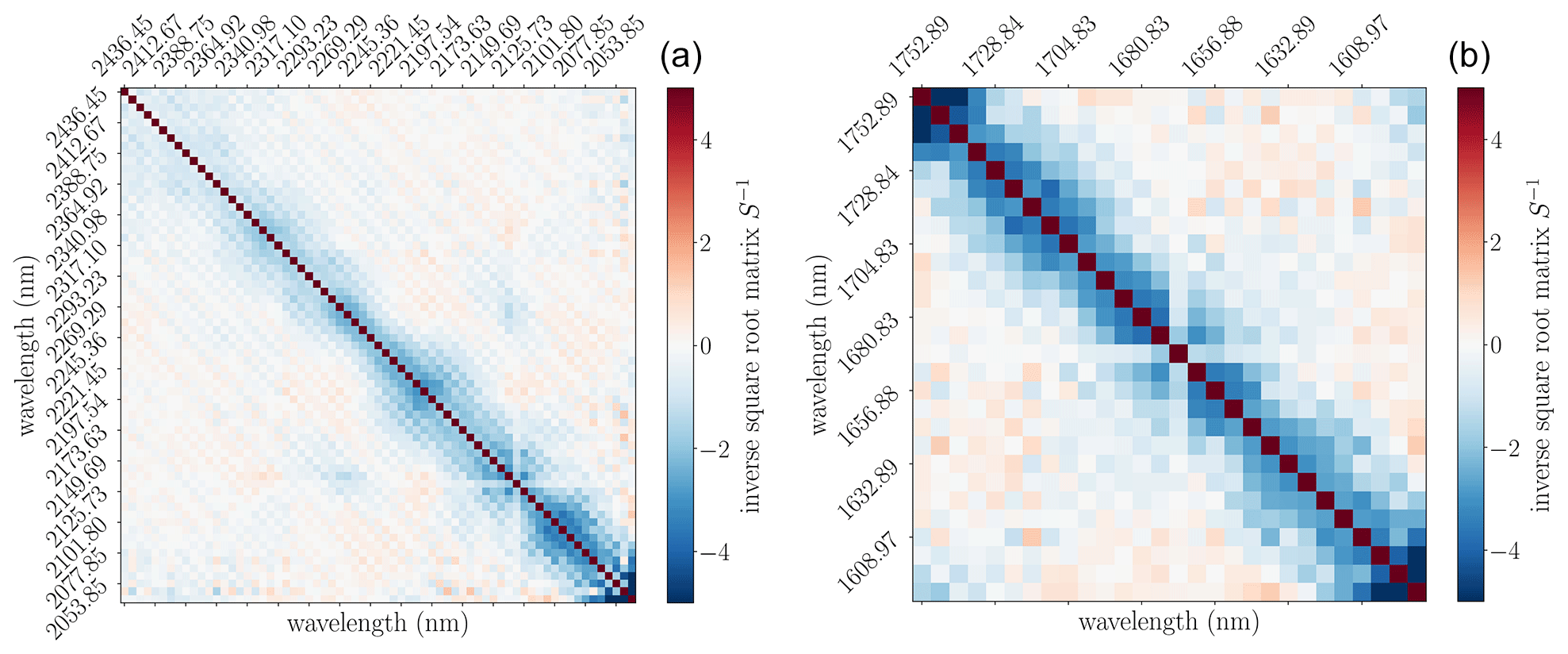
\begin{matrix} (6) & min_{x} ‖ S^{- 1} (y - Φ (x)) ‖^{2} . \end{matrix}

https://amt.copernicus.org/articles/16/4195/2023/amt-16-4195-2023-f04

Figure 4Scene 09 inverse square root matrix of C: (a) 4100–4900 cm⁻¹ (4K) and (b) 5700–6300 cm⁻¹ (6K) spectral range. The background area was defined outside of the pixels: $along-track = (6300, 6670)$ ; $across-track = (180, 285)$ . Note that beside the bad HySpex pixel mentioned in Fig. 2 at 5992.74 cm⁻¹ there appears to be another suspect pixel at 4691.04 cm⁻¹.

Download

2.3.2 Enhancement estimates for the nonlinear solvers

A scene-averaged background spectrum, excluding ground pixels around the suspected CH₄ sources, is employed to estimate actual H₂O, CO₂, and CH₄ background concentrations. The CO₂ background level of the scene is inferred from the 1.6 and 2 µm bands via a multi-interval (4K and 6K spectral windows) fit. For scene 09 and scene 11, a scaling factor of ${\tilde{α}}_{{CO}_{2}} = 0.96$ (≈385 ppm) and ${\tilde{α}}_{{CO}_{2}} = 0.93$ (≈375 ppm) was determined for the initial guess, respectively. Due to the degeneracy between H₂O and the reflectivity polynomial at HySpex's spectral resolution, the scene-averaged H₂O scaling factor constitutes an effective parameter partly capturing low-frequency components in the spectrum. The scene-averaged CH₄ background profile was found to be within 5 % of the initial guess of 1875 ppbv; hence it is not (pre)scaled.

The state vector x for the CH₄ enhancement fit comprises the CH₄ scaling factor and the coefficients for a second-order reflectivity polynomial per spectral interval $x = (α, r_{0}, r_{1}, r_{2})$ . In this setup the parameter α only applies to the plume component (up to 2.0 km) of the CH₄ optical depth

\begin{matrix} (7) & τ_{{CH}_{4}} = τ_{bg} + α τ . \end{matrix}

This setup was found to be robust toward lower SNR values and less susceptible to correlations among state variables, which in turn enhances the condition number of the Jacobian matrix.

The actual CH₄ total column is then given by the background concentration plus the retrieved enhancement and includes corrections for light path modifications via the prefitted scene-averaged background CO₂ given by

\begin{matrix} (8) & N_{{CH}_{4}} = N_{bg} + \frac{α}{{\tilde{α}}_{{CO}_{2}}} \hat{N} (z_{0}), \end{matrix}

with

\begin{matrix} (9) & \hat{N} (z_{0}) = \int_{z_{0}}^{z_{pl}} n_{pl} (z) d z \end{matrix}

and z₀ representing the bottom of the atmosphere and n_pl the plume's number density. This approach assumes that the CO₂ profile upon which ${\tilde{α}}_{{CO}_{2}}$ is estimated corresponds to the true profile and that ${\tilde{α}}_{{CO}_{2}}$ is 1 in absence of scattering.

2.4 Linear solvers

In contrast to nonlinear fitting schemes, linear solvers for x can only be used when equations can be expressed as a linear combination of the variables in x. To utilize such methods, it is usually required to linearize the forward model with respect to the variables of interest.

2.4.1 Linear least squares (LLS)

Assuming that the increase in optical depth caused by the plume, τ, is relatively small, the BIRRA forward model from Sect. 2.3 is linearized with respect to α by approximating the transmission spectrum of the plume by Taylor expansion according to

\begin{matrix} (10) & \exp (- τ) \approx (1 - α τ) . \end{matrix}

The linear least squares problem of M measurements can then be formulated according to

\begin{matrix} (11) & min_{x} ‖ y - Φ x ‖, \end{matrix}

where the model functions in Φ for the linear parameters of the state vector $x = (r_{0}, r_{0} α)$ are given by

\begin{matrix} (12) & ϕ_{1} = \frac{\cos (θ)}{π} I_{sun} T^{↓} T^{↑} \otimes S, \\ (13) & ϕ_{2} = - \frac{\cos (θ)}{π} I_{sun} T^{↓} T^{↑} τ \otimes S . \end{matrix}

It is important to note that in this setup the reflectivity coefficient r₀ is present in two elements of the state vector. In order to avoid this degeneracy and allow for higher-order reflectivity polynomials in the fit, which are required for large spectral intervals, the retrieval is performed in two steps. First, only the reflectivity coefficients are fitted, while in a second step only α is estimated with the prefitted reflectivity coefficients provided as input. The setup can be complemented by de-weighting individual pixels in the albedo fit that are impacted by methane. This approach minimizes interference between the two fits, preventing the reflectivity polynomial from capturing absorption of CH₄.

Another aspect that should be kept in mind is that since $1 - α τ \leq \exp (- α τ)$ for α≥0 the linearized model underestimates the CH₄ enhancement for a given optical depth τ compared to the nonlinear setup.

2.4.2 Matched filter (MF)

The MF is a well-established method for estimating molecular concentration enhancements from hyperspectral sensors, with numerous studies supporting its effectiveness (Villeneuve et al., 1999; Funk et al., 2001; Thorpe et al., 2013; Thompson et al., 2015). The linear enhancement factor is inferred by perturbing an average (background) radiance spectrum μ with a known target spectrum t. The approach is analogous to that used by Thompson et al. (2015), where CH₄ enhancements are estimated by linearly scaling a target signature that perturbs the mean radiance:

\begin{matrix} (14) & α_{i} (y) = \frac{(t (μ))^{T} C^{- 1} (y_{i} - μ)}{\sqrt{(t (μ))^{T} C^{- 1} (t (μ))}} . \end{matrix}

This equation constitutes the linear minimizer that solves the Gaussian log likelihood:

\begin{matrix} (15) & \begin{aligned} min_{α_{i}} ‖ C^{- 1 / 2} d ‖^{2} & with d = y_{i} - (μ + α_{i} t (μ)) \\ and t (μ) = - μ τ . \end{aligned} \end{matrix}

The method assumes that the measured spectrum can be represented as a linear superposition of the CH₄ plume's optical depth and the mean unperturbed radiance μ and tests an observed vector y_i against a base vector while accounting for the background covariance C. The mean background spectrum μ and C are computed per scene; C⁻¹ is approximated by decomposing C into eigenvalues and eigenvectors (Thompson et al., 2015, Eqs. 6–8).

In order to improve accuracy, a per-measurement target spectrum is computed, which accounts for the pixel's albedo (Foote et al., 2020, II. Methods, C.). This normalized matched filter includes an albedo factor r_i for each measurement spectrum according to

\begin{matrix} (16) & d_{r} = y_{i} - (μ + r_{i} α_{i} t (μ)) with r_{i} = \frac{y_{i}^{T} μ}{μ^{T} μ} . \end{matrix}

However, the MF method has its limitations; for example, it suffers from a heterogeneous background and correlation between the plume and the background which limits the detection quality even for strong plumes (Theiler and Foy, 2006). According to Guanter et al. (2021), a way to mitigate the effect is by k-means clustering of the scene. This approach reduces within-class variance, which in turn should minimize the albedo sensitivity of α. In the so-called cluster-tuned matched filter, instead of a single background covariance statistic, a per-cluster background statistic C_i is computed (Thorpe et al., 2013; Nesme et al., 2020).

2.4.3 Singular value decomposition (SVD)

The retrieval of methane enhancements from hyperspectral AVIRIS data using singular vectors of the observed spectrum plus a target signature was first demonstrated by Thorpe et al. (2014). The SVD method is well suited for parameter estimation from moderately resolved spectral data because it allows us to consider only the most significant components of the spectrum while preserving the main spectral information.

The orthogonal singular vectors are obtained from HySpex spectra that are not impacted by the plume. The matrix containing the scene's log-space background spectra is decomposed into USV^T, where $U \in R^{m \times m}$ and $V \in R^{n \times n}$ are unitary matrices, and $S \in R^{m \times n}$ is a diagonal matrix. The target signature (spectrum) is represented by the CH₄ plume's optical depth τ, which is computed with Py4CAtS.

The basic idea is analogous to the MF, i.e., to represent the general variability in spectral radiance by a linear combination of singular vectors and a target signal. The minimization problem is then given by

\begin{matrix} (17) & min_{w} ‖ y - A w ‖^{2} with A w = \sum_{k}^{N} u_{k} w_{k} + t w_{{CH}_{4}}, \end{matrix}

where A represents the concatenated matrix of the first N columns of the unitary matrix U (see Fig. 5). The vector w contains the corresponding weights, with $α = w_{{CH}_{4}}$ scaling the contribution of enhanced methane in the lowest atmospheric layers t=τ. In the cluster-tuned variant, the background spectra are clustered by k-means clustering, and the SVD is performed for each cluster separately. The respective base vectors per cluster are then used in the linear fit.

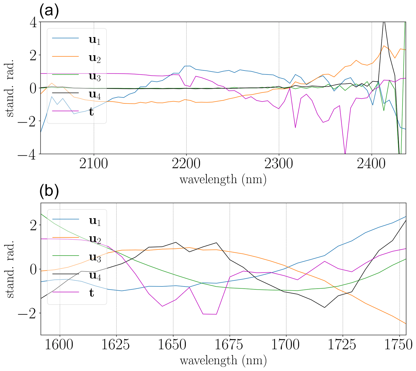
https://amt.copernicus.org/articles/16/4195/2023/amt-16-4195-2023-f05

Figure 5Standardized singular vectors u and the methane plume's target signature t in 4K (a) and 6K (b) spectral intervals, respectively. Standardization removes the mean and scales to unit variance. The u vectors are defined by the SVD and the t vector by the radiative transfer model Py4CAtS. Modeling the plume's optical depth with the same tools and for an equivalent setup (<2 km) is crucial for comparability with the nonlinear BIRRA setups.

Download

2.4.4 Spectral signature detection (SSD)

A straightforward approach to identify methane absorption is the SSD, which compares the ratio of spectral residual norms to produce a score. Unlike other methods, this approach does not require any radiative transfer calculations, lookup tables, or initial guess information – only calibrated sensor data for a specific interval.

The algorithm is based on a simple polynomial fit of spectral pixels and the calculation of spectral residuals. The idea behind this method is similar to the continuum interpolated band ratio (CIBR) from Green et al. (1989) and Thompson et al. (2015, Eq. 2), which also measures absorption depths (Pandya et al., 2021). The method splits the spectral interval into pixels where CH₄ is absorbed and where it is not (or only weakly). A polynomial of degree P is fitted to the M out-of-band pixels:

\begin{matrix} (18) & min_{x} | | y - P x | |^{2} with P \in R^{m \times (P + 1)} . \end{matrix}

Next the residual norms for the in-band and out-of-band pixels are computed. The ratio of the residual norms yields an absorption band depth score for each observation which indicates variations in the CH₄ absorption given that the in-band and out-of-band pixels were properly chosen.

The algorithm constitutes a fast scheme which can also be applied for real-time detection of enhancements, e.g., determine whether or not a CH₄ ventilation shaft is active at the time of instrument overpass. When a zero-order polynomial is used for the out-of-band fit, the method is comparable to the CIBR algorithm. However, by using higher-order polynomials, the method can model the surface reflectivity and other interfering species more precisely, especially over larger spectral intervals.

3 Results

This section presents the results for the CH₄ estimates over the Pniówek V shaft(s). Except as otherwise stated, the retrievals were performed on 3×3 pixels averaged spectra in order to increase the signal-to-noise ratio and thereby reduce clutter of the CH₄ fits across pixels.

3.1 NLS and SLS fits

Figure 6 shows the results of the classical BIRRA NLS fit. The position of the source is indicated by the intersection of the dashed line. The fits reveals a significant enhancement of CH₄ in both spectral intervals downwind of the ventilation shaft. However, both BIRRA configurations exhibit biases, with the SLS fit displaying a somewhat more pronounced sensitivity to surface variations (therefore not shown). As depicted in Fig. 6, the combination of multiple spectral intervals can alleviate these adverse effects to a considerable extent, and the downwind shape of the plume is captured better (see Table 2).

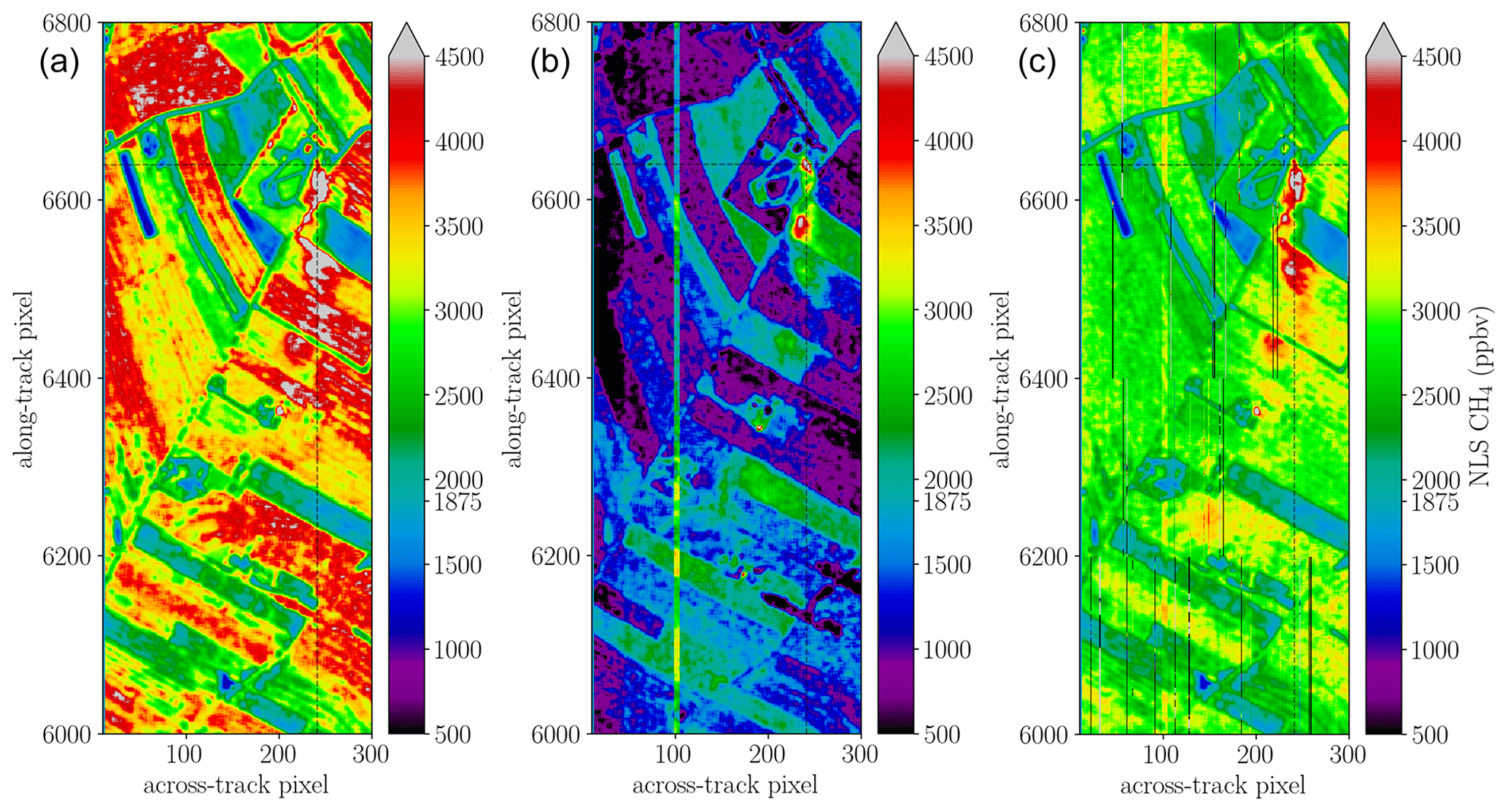
https://amt.copernicus.org/articles/16/4195/2023/amt-16-4195-2023-f06

Figure 6Methane enhancements for 3×3 spatially averaged HySpex observations in the (a) 4150–4900 cm⁻¹ (4K) interval and the (b) 5700–6300 cm⁻¹ (6K) range. (c) Multi-interval fit, i.e., combining the 4K and 6K ranges (4K6K). Note that the former two NLS fits suffer from albedo correlations with methane in opposite direction.

Download

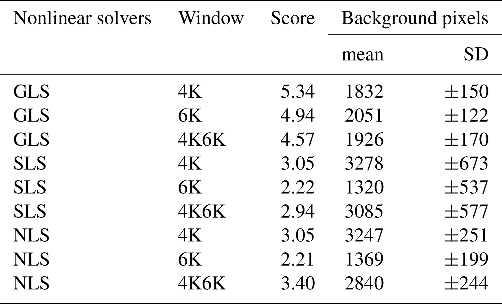
Table 2Mean and standard deviation (SD) for the background pixels of the t test. Relating the standard deviation to the mean is a good indication of the accuracy and precision of a method.

Download Print Version | Download XLSX

3.2 GLS fits

Figure 7 displays the retrieved columns using the generalized least squares (GLS) fit from averaged spectra for scene 09 in the 4K and 6K intervals. Compared to other methods, it reduces the correlation between the methane enhancement and surface reflectivity significantly, resulting in a more distinct plume signal and less background clutter.

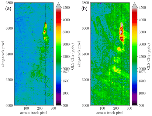
https://amt.copernicus.org/articles/16/4195/2023/amt-16-4195-2023-f07

Figure 7Methane plume depicted for the single-window covariance-weighted fits for scene 09. The background pixel concentration is rather stable in the 4K interval depicted in panel (a), while there is still some overestimation of CH₄ in the 6K range in panel (b) which might partly be caused by the bad pixel close to the methane absorption band (see Figs. 2 and 4).

Download

Figure 8 shows the multi-window covariance-weighted GLS fits for scene 09 and 11. In both cases the retrieval yields a distinct plume that separates well from background clutter. The figure depicts the impact of decreasing ground pixel resolution (from higher altitudes) on the inferred concentrations as enhancements are less pronounced for scene 11. However, this could also partly be attributed to a decreased amount of emissions since the observation was taken at another point in time. Furthermore, winds could have changed as the plume's shape is different compared to scene 09.

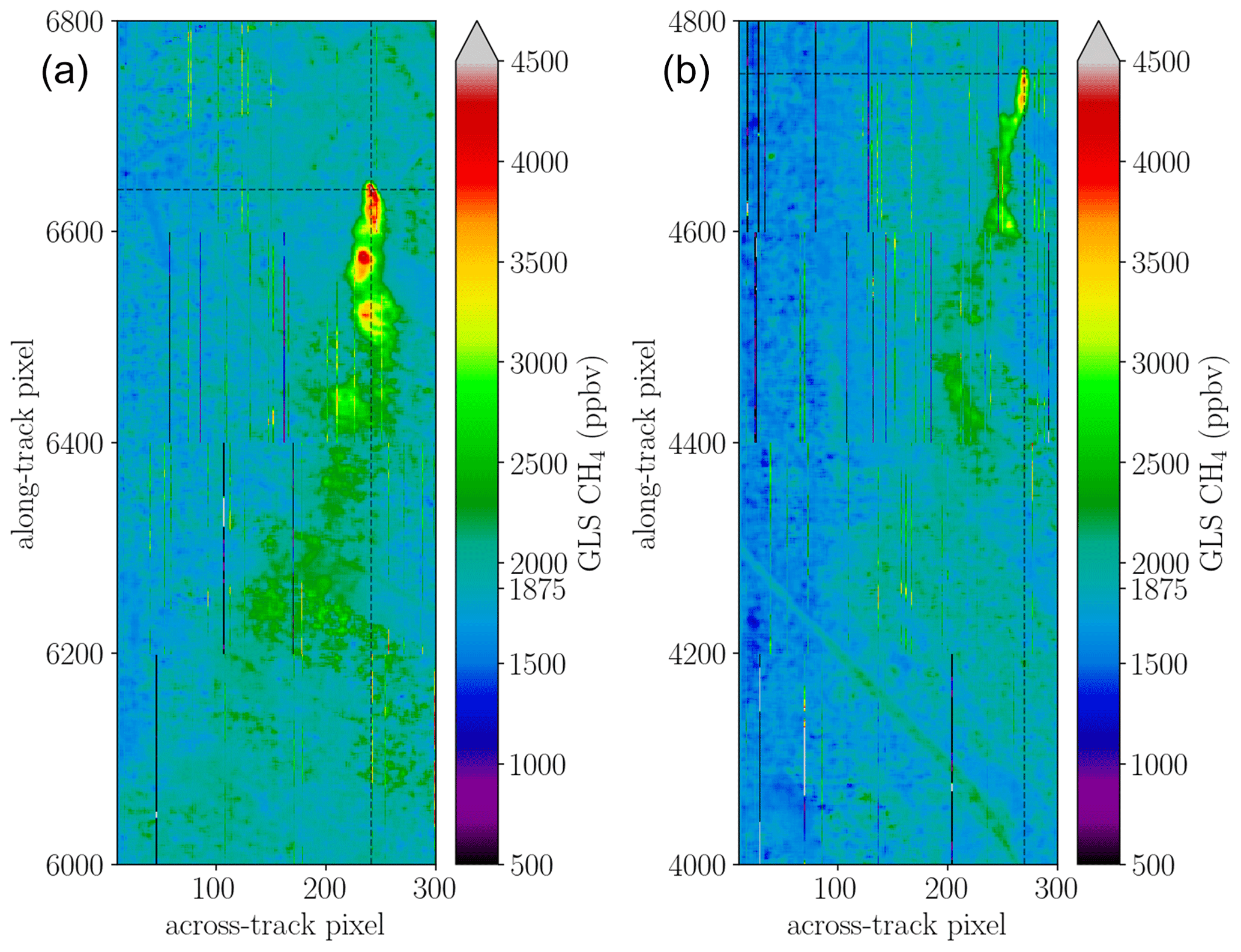
https://amt.copernicus.org/articles/16/4195/2023/amt-16-4195-2023-f08

Figure 8(a) Multi-window (4K6K) retrieval output for scene 09 and (b) enhancements for scene 11. The stripe pattern in the along-track direction is a multi-window retrieval artifact.

Download

Figure 9 depicts the fits from individual (non-averaged) HySpex spectra for scene 09 and 11 for the GLS multi-window retrieval setup. The single-pixel total columns are more affected by retrieval noise caused by the lower signal-to-noise ratio (SNR), which varies significantly over different surface types. However, the method still identifies elevated methane concentrations.

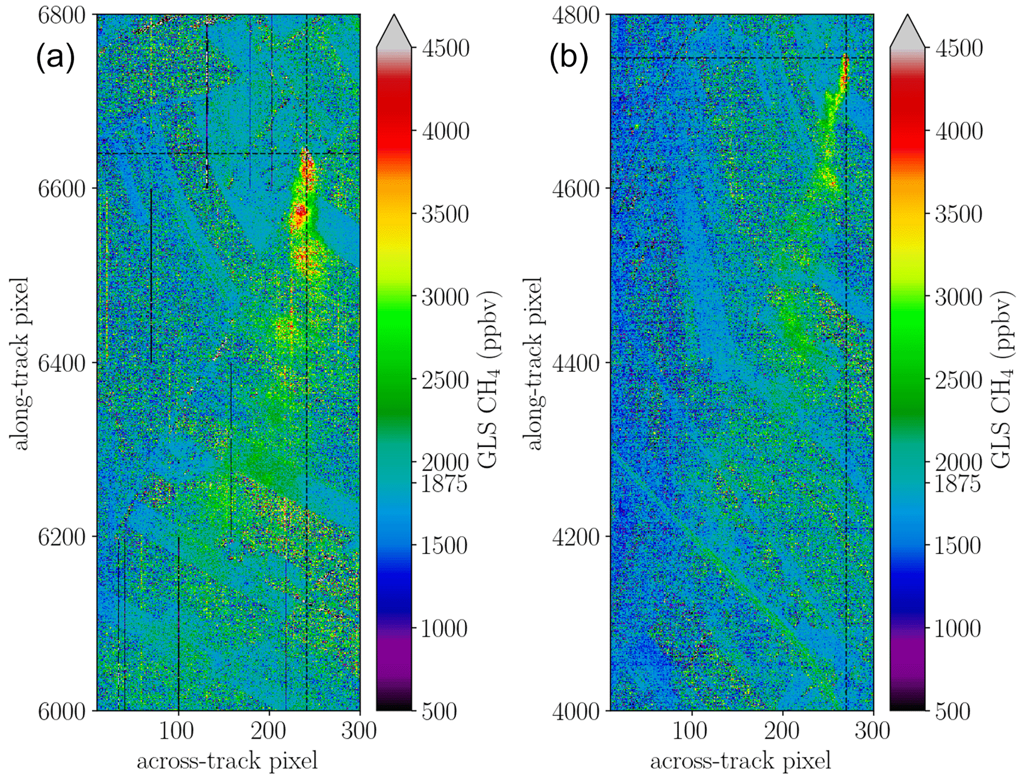
https://amt.copernicus.org/articles/16/4195/2023/amt-16-4195-2023-f09

Figure 9In the single-pixel spectra depicted for (a) scene 09 and (b) scene 11, retrieval noise is significantly dependent on the underlying surface.

Download

3.3 MF fits

The albedo-normalized, cluster-tuned, and classical matched filters are examined for scene 09. Figure 10 shows that all three variants are able to identify the methane plume, although absolute CH₄ concentrations differ in certain parts of the scene. The cluster-tuning MF variant in the middle panel yields more homogeneous enhancements downwind across various surface types, but pixels along class boundaries such as streets show some artifacts.

https://amt.copernicus.org/articles/16/4195/2023/amt-16-4195-2023-f10

Figure 10(a) Albedo-normalized MF, (b) the cluster-tuned variant, and (c) the classical MF fit shown for the 4K interval (4100–4900 cm⁻¹).

Download

3.4 SVD fits

The SVD-based retrieval method illustrated in Fig. 11 is able to identify elevated levels of CH₄ in the HySpex spectrum. The method yields consistent results for both spectral intervals, employing four base vectors and the CH₄ Jacobian for the lowest 2 km (see Fig. 5). Including more than four base vectors significantly increases the condition number of A as column five interferes with the methane signal. The plume is also identified for the purely data-driven approach, where the base vector mimicking the CH₄ absorption (the fifth column in U) is used instead of the CH₄ spectrum. Thus, this approach does not require any forward model and is hence purely data-driven. Cluster tuning in general improves the fit due to a reduction in variance within each cluster; however, the results become more sensitive to the selected number of base vectors. It was found that within a cluster the number of base vectors required to resemble A should be reduced.

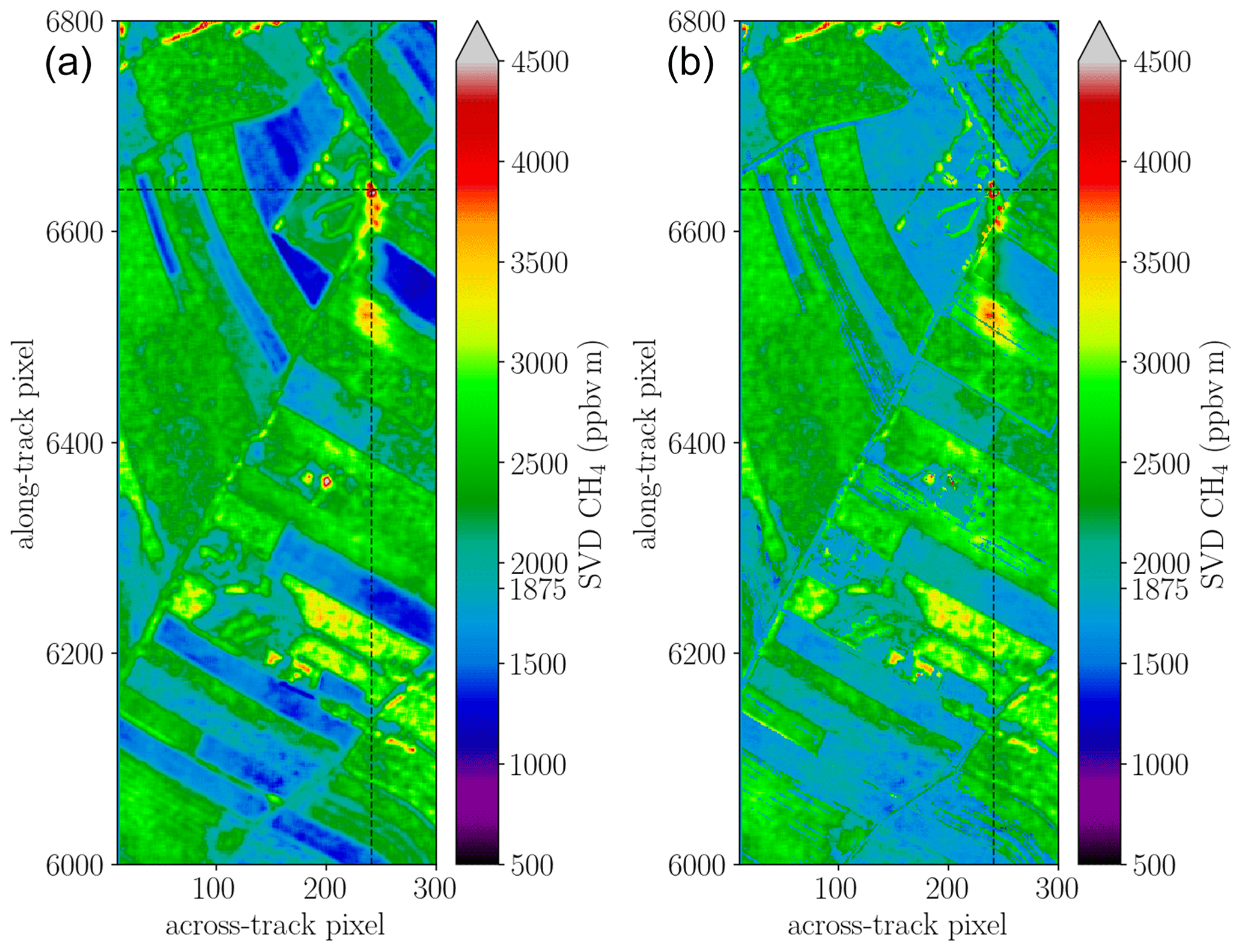
https://amt.copernicus.org/articles/16/4195/2023/amt-16-4195-2023-f11

Figure 11(a) Standard SVD fit and (b) background cluster-tuned SVD, both for the 6K spectral range. Three clusters reduce background clutter but suppress some enhancements close to the source. However, also false positives like the spot around the coordinate (200,6350) are diminished.

Download

3.5 LLS fits

The linear least squares fit is able to identify CH₄ enhancements, although it differs significantly in the absolute values in the 4K and 6K spectral range (see Fig. 12). As pointed out in Sect. 2.4.1, the method is prone to underestimating enhancements. Moreover, the selected weights for the reflectivity coefficient fit were found to impact the CH₄ result. However, for the sake of simplicity and since the optimal selection of weights was not clear initially, no weighting was applied. Similar to its nonlinear counterpart (NLS) the fit is also affected by albedo-related offsets in opposite directions in the two intervals. However, relative enhancements between plume and background values are rather similar.

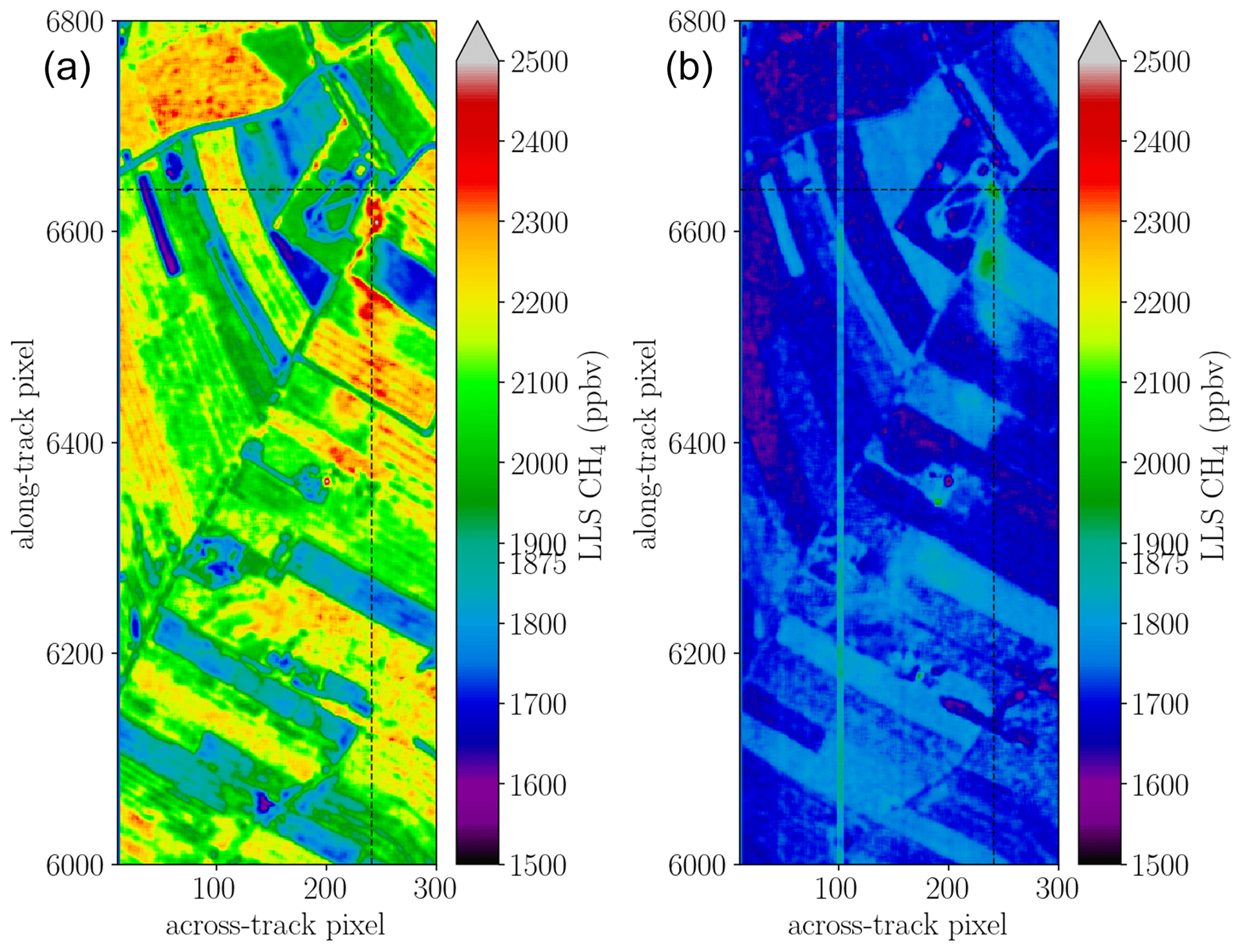
https://amt.copernicus.org/articles/16/4195/2023/amt-16-4195-2023-f12

Figure 12CH₄ enhancements for scene 09 estimated with the LLS setup. The results in panel (a) show the results for the 4K spectral window, while panel (b) shows the 6K outcome. In the latter method, the methane enhancements are less pronounced, but the reflectivity-related bias is also smaller.

Download

3.6 SSD fits

In Fig. 13, results for the SSD method are shown. The results show that relative variations are more pronounced in the zero-order fit, while the higher-order fit better captures the downwind plume by suppressing background clutter.

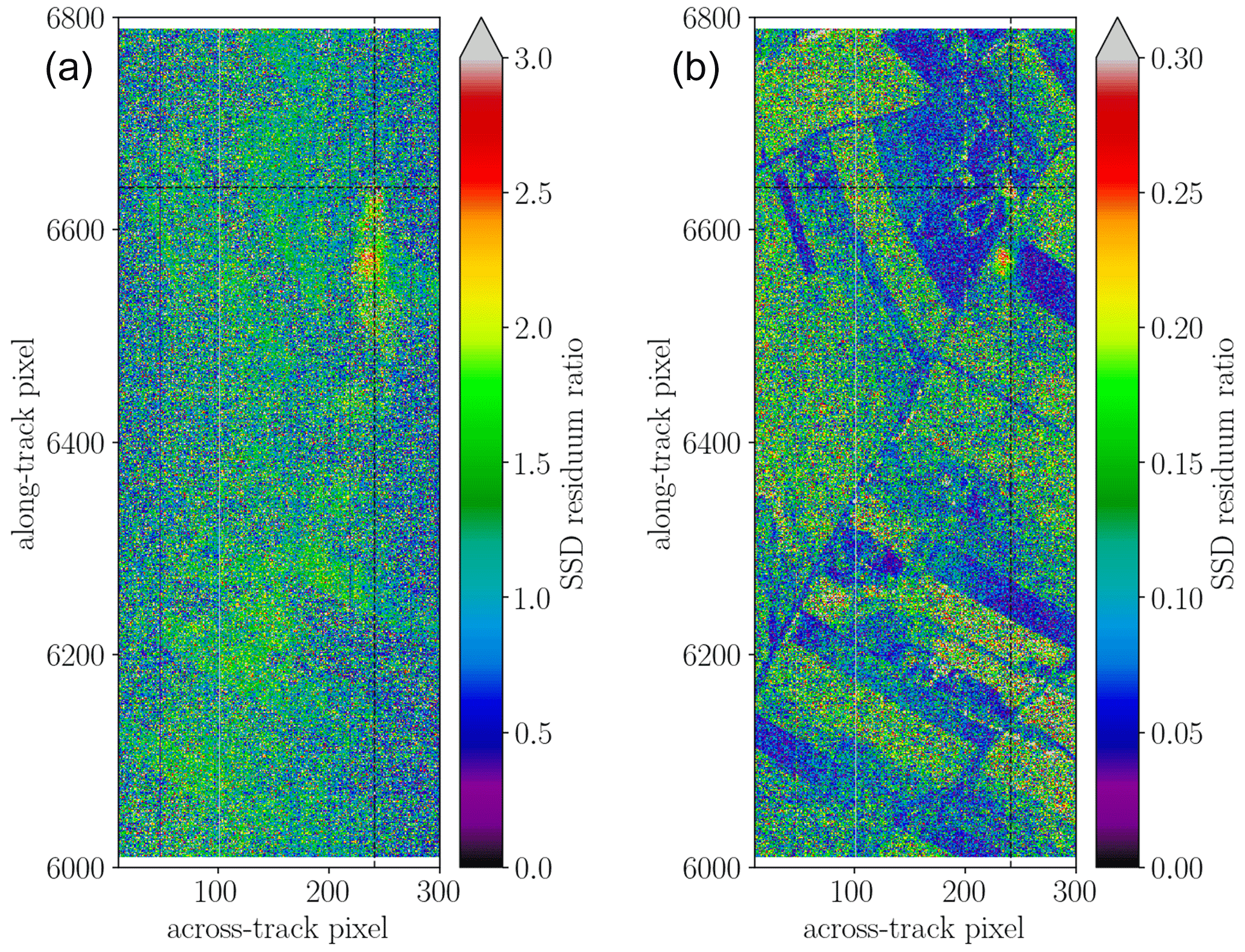
https://amt.copernicus.org/articles/16/4195/2023/amt-16-4195-2023-f13

Figure 13The ratio of the spectral residuals in the 6K range for the in-band and out-of-band pixel is depicted. In panel (a) the in-band residuals were computed with respect to a quadratic polynomial, while in panel (b) a constant was used.

Download

It is important to note that the method yields better results for the 6K absorption since the 4K absorption features are distributed over a larger spectral range which causes more uncertainty in the out-of-band polynomial fit since many pixels need to be omitted.

3.7 Statistical significance of results

In order to provide a more quantitative measure on the quality and confidence of the fits, a Student t test was applied to the results (Varon et al., 2018). The test helps to measure how well the plume is represented with respect to the background for a given retrieval setup. This is accomplished by testing for pixels that contradict the null hypothesis, which assumes that all pixels belong to the background (methane concentration). Moreover, samples need to be independent and identically normally distributed (Bruce et al., 2020).

The null hypothesis was rejected at the 1 % significance level, which can be considered a strong evidence. Although some fit results may ask for a tighter significance level in the t test to isolate the plume and get rid of most outliers, for the sake of comparison 1 % is used throughout this study.

Figure 14 depicts the result of the t test applied to the retrieval output for scene 09 and 11 from the covariance-weighted nonlinear solver (GLS) in the 4K range. The plume is well pronounced, and the test is able to isolate enhanced CH₄ values from the background. In particular, the higher-ground-resolution scene 09 shows almost no outliers at the selected significance level, indicating that the depicted values occur only in ≤1 % of the cases, assuming the null hypothesis (background methane concentrations) holds.

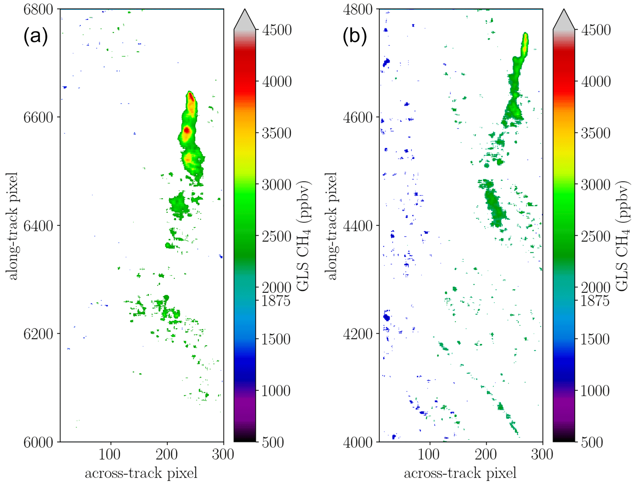
https://amt.copernicus.org/articles/16/4195/2023/amt-16-4195-2023-f14

Figure 14Plume pixels according to the Student t test for the nonlinear multi-window GLS fit. Panel (a) shows scene 09, while panel (b) shows scene 11.

Download

The Student t test was also applied to the linear solvers, with results reported in Fig. 15. The test was performed with the same significance level set for the previous cases. Each of the linear methods provides enough pixels within the confident range to isolate the plume pixels. While MF provides the most accurate enhancement values compared to the GLS (see Fig. 14), the SVD better captures the downwind plume; however, peak enhancements are ≈30 % lower. The LLS method does capture the downwind plume but is much less sensitive to enhancement as it significantly underestimates these.

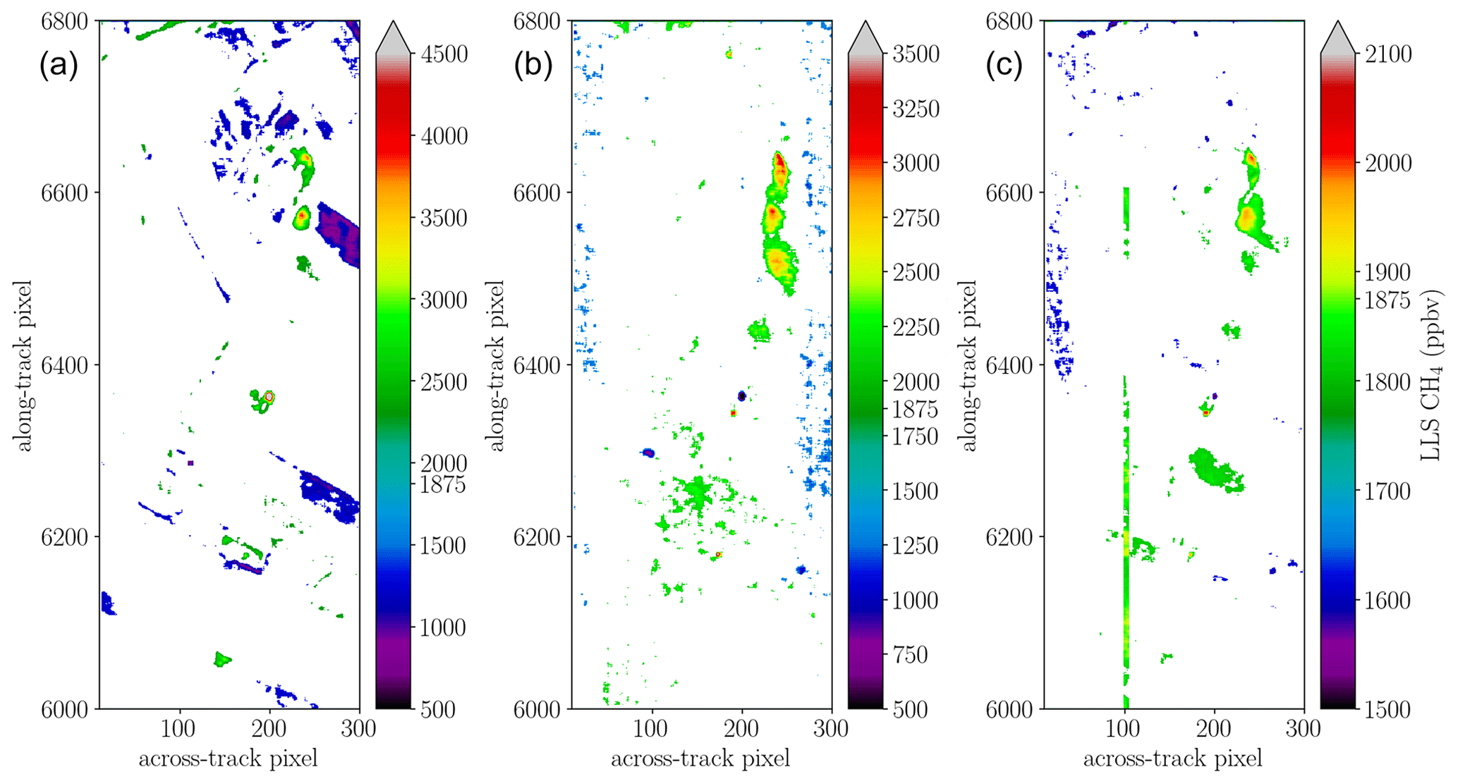
https://amt.copernicus.org/articles/16/4195/2023/amt-16-4195-2023-f15

Figure 15Plume pixels identified by the t test in scene 09 for the different linear schemes. Note that the color scale was adapted. (a) Classical MF output from the 4K range, (b) plume pixels according to the SVD method in the 6K interval, and (c) the LLS fit in 6K.

Download

3.8 Errors and correlations

In general the retrieval's fit quality is assessed with respect to the discrepancy between the measurement y and the modeled spectrum I according to $σ = ‖ y - I (\hat{x}) ‖$ , also known as the residual norm. In order to get the uncertainties in the estimates of the model parameter $\hat{x_{i}}$ for a particular fit, the residual norm is multiplied by the least squares covariance matrix:

\begin{matrix} (19) & V = \frac{σ^{2}}{M - N} {(J^{T} J)}^{- 1} with \hat{x_{i}} \pm \sqrt{V_{i i}}, \end{matrix}

with J representing the Jacobian matrix for the state vector $\hat{x}$ .

The errors of the individual state vector parameters are represented in the square root of the diagonal elements of V. The standard error $\sqrt{V_{11}}$ for the CH₄ scaling factor is shown in Fig. 16. The uncertainty varies with different surface types according to Eq. (19). A different way to evaluate the quality of the retrieval for a scene is to estimate the fit error from the variability of pixels identified as background by the t test. This method calculates a score by comparing the means of pixels from the target area and the background area and dividing this by the standard deviation of the background. These values are also obtainable for all the linear fit variants.

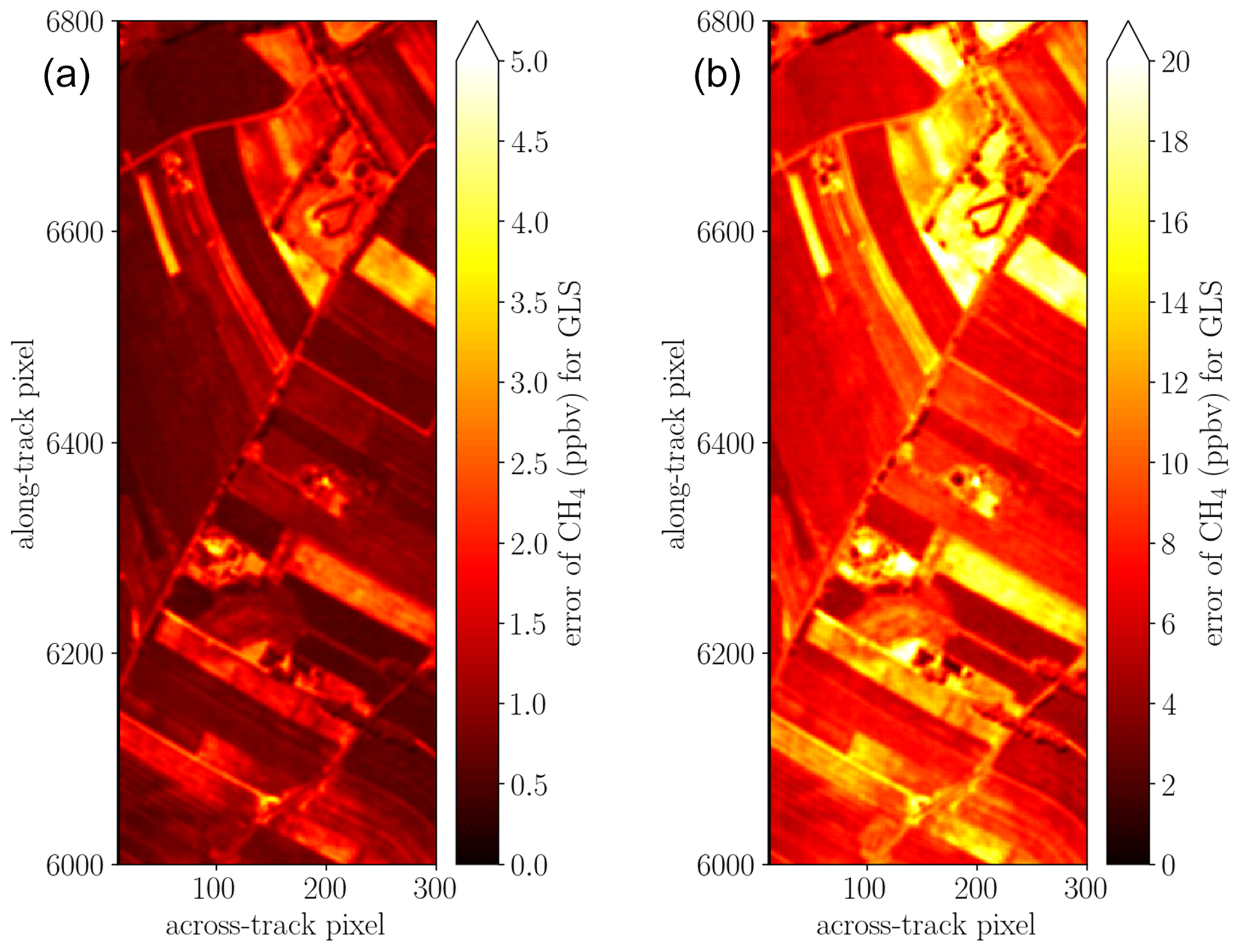
https://amt.copernicus.org/articles/16/4195/2023/amt-16-4195-2023-f16

Figure 16Uncertainties in the estimated CH₄ according to Eq. (19) for the covariance-weighted fit in the (a) 4K and (b) 6K spectral windows. The 6K range shows larger errors as it contains less than half the number of pixels than the 4K window. Beside the higher variances, the bad pixel close to the methane lines around 1.6 µm also increases the spectral residual norm.

Download

Tables 2 and 3 present the findings of this analysis for the nonlinear and linear solvers, respectively. The analysis shows that the GLS fit performs best and that SLS and NLS yield similar results, while the MF scores highest amongst the linear solvers. In accordance with Fig. 16, fits in the 4K window score higher compared to the 6K. The less sensitive the retrieval is to CH₄ enhancements, the less variations will be observed in the background. Therefore, the standard deviation in the last column should not be overemphasized in the evaluation of the setups.

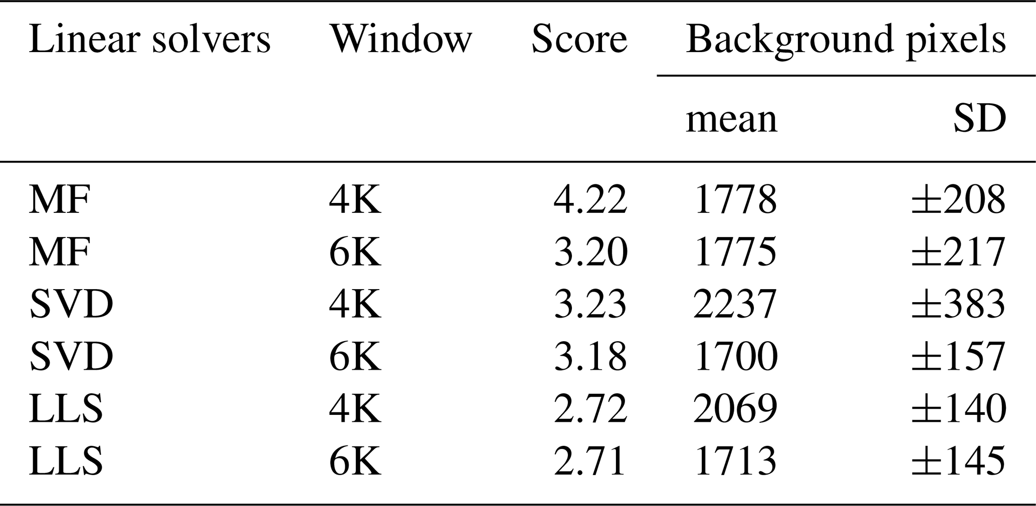
Table 3Same as Table 2 but for the linear retrieval setups.

Download Print Version | Download XLSX

Figure 17 shows the correlation matrix of the retrieval outputs for the different solvers and spectral intervals. It reveals that most solvers have rather good correlations with the GLS solver (sort of benchmark), particularly in the 4K and multi-window 4K6K spectral ranges. Moreover, the GLS, MF, and SVD show blocks of high correlation. Blue colors indicate that inferred concentrations tend to move in opposite directions, which is the case for example in the single-window NLS fits shown in Fig. 6.

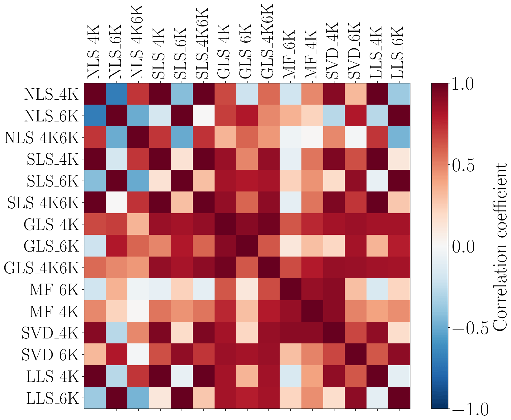
https://amt.copernicus.org/articles/16/4195/2023/amt-16-4195-2023-f17

Figure 17Pearson correlation coefficients for inferred methane from scene 09 for the nonlinear and linear solvers in the two examined spectral intervals.

Download

4 Discussion

The study found that nonlinear setups which utilize background pixel covariance statistics (GLS) are suited to quantify CH₄ concentrations with good accuracy and precision and should also allow us to quantify emissions. The NLS and SLS fits encounter challenges due to degeneracies between the surface reflectivity and the broad-band molecular absorption signal at the HySpex resolution. In accordance with Borchardt et al. (2021) and Guanter et al. (2021), surface brightness and homogeneity were found to be important factors in detecting and quantifying methane plumes. The retrieval noise can vary significantly depending on surface characteristics. A given type of surface can lead to a positive bias in one spectral window, while the opposite may be true in another window (see Fig. 9).

In order to scan for potential CH₄ leakages on large datasets with millions of pixels, linear solvers such as the SVD, MF, or LLS are more appropriate due to their significantly higher speed (Thompson et al., 2015). While the iterative setups require roughly 1 s per fit, the linear methods are up to 3 orders faster. In particular, the SVD and MF solvers yield enhancements that often agree well with the more sophisticated nonlinear methods, although their sensitivity can be significantly hampered by the lack of uniformity in background reflectance (Thorpe et al., 2014; Foote et al., 2020).

The LLS fit ignores background statistics, and hence the inversion suffers from albedo correlations similar to its nonlinear counterparts. The fit also significantly underestimates enhancements, although it is able to capture parts of the pattern.

Polynomials up to the second order were able to capture the enhanced methane signal in the rather simple SSD method. The selection of an adequate polynomial needs to consider the width of the spectral interval and its surface reflectivity. Moreover, the method is not designed to quantify methane but only allows for the detection of anomalies in the spectral residuum.

Cluster tuning of linear retrieval setups can help to mitigate background clutter and surface-reflectivity-induced biases (Nesme et al., 2020), especially if large background areas are selected. Predicting the right cluster for pixels impacted by the methane plume is crucial for this method in order to improve fit results. Cluster tuning can moreover be a beneficial preprocessing step as it allows us to reduce the base vectors per cluster in the SVD method so that fewer base vectors are sufficient to model the background spectrum. However, in this case a separate model matrix A needs to be compiled for each cluster.

While linear methods are well suited to survey vast datasets and pinpoint potential sources, iterative solvers such as BIRRA are adequate to quantify enhanced concentrations at known locations as the slower speed is not of much concern for some thousands of observations.

5 Conclusions

The study examines the feasibility of methane retrievals from hyperspectral imaging observations for various retrieval methods. It was found that localized CH₄ enhancements close to the ground can be quantified from HySpex airborne observations. The generalized BIRRA retrieval is well suited to investigate potential methane emissions. The statement is underpinned by the relatively low background variations and distinct CH₄ enhancement pattern in the surface-albedo covariance-weighted BIRRA fits in (see Figs. 7 and 8 and Table 2).

The BIRRA NLS and SLS fits were found to be sensitive to spectral variations in the albedo, leading to surface-type-dependent biases known from previous studies utilizing data from hyperspectral sensors. This effect is more pronounced for single spectral intervals but less evident when multiple intervals are combined.

The linear estimators proved to be highly efficient and effective for many cases, making them suitable in the survey of large hyperspectral datasets. The well-established SVD and MF method produced results that often agree well with the BIRRA inferred enhancements; however, the sensitivity is lower. The LLS method turned out to be the least sensitive one. For detection purposes the SSD was found to be a useful tool.

In conclusion, covariance-weighted methods are able to quantify methane enhancements from hyperspectral SWIR observations at high spatial resolution with good accuracy. In particular, the GLS solver is suited to capture enhancements with an accuracy that should allow for emission estimation. Considering the significant speedup and reasonable accuracy of the linear methods MF and SVD, both constitute a valuable tool in examining plumes on vast datasets.

The methods are also applicable to spaceborne sensors, which will be considered in a next step. Overall, the new Python version of the BIRRA code used in this study turned out to be a flexible toolbox for prototyping.

Code availability

Parts of the code are published via the Py4CAtS software suite (see Schreier et al., 2019, https://doi.org/10.3390/atmos10050262).

Data availability

The data used in this study are available from the corresponding author upon request.

Author contributions

PH developed and implemented the retrieval setups and analysis tools and wrote the manuscript. FS originally designed and developed the software package Py4CAtS and supported the data evaluation. CHK conceived the experimental setup and conducted the data acquisition of the airborne measurements. AB performed the instrument calibration and level 0–1 processing. CHK and AB contributed the experimental setup. DC gave valuable advice for the cluster-tuning approach and provided spectral unmixing data for the verification of the SVD and MF results. All authors reviewed the manuscript.

Competing interests

The contact author has declared that none of the authors has any competing interests.

Disclaimer

Publisher's note: Copernicus Publications remains neutral with regard to jurisdictional claims in published maps and institutional affiliations.

Special issue statement

This article is part of the special issue “CoMet: a mission to improve our understanding and to better quantify the carbon dioxide and methane cycles”. It is not associated with a conference.

Acknowledgements

We thank Thomas Trautmann and Peter Haschberger for valuable criticism of the manuscript. Furthermore, we thank Konstantin Gerilowski for initiating cooperation with the CoMet campaign and Andreas Fix, the campaign leader, for the support and coordination.

Review statement

This paper was edited by Justus Notholt and reviewed by David R. Thompson and two anonymous referees.

References

Anderson, G., Clough, S., Kneizys, F., Chetwynd, J., and Shettle, E.: AFGL atmospheric constituent profiles (0–120 km), Tech. Rep. TR-86-0110, AFGL, https://apps.dtic.mil/sti/pdfs/ADA175173.pdf (last access: 1 September 2023), 1986.

Ayasse, A. K., Thorpe, A. K., Roberts, D. A., Funk, C. C., Dennison, P. E., Frankenberg, C., Steffke, A., and Aubrey, A. D.: Evaluating the Effects of Surface Properties on Methane Retrievals Using a Synthetic Airborne Visible/Infrared Imaging Spectrometer next Generation (AVIRIS-NG) Image, Remote Sens. Environ., 215, 386–397, https://doi.org/10.1016/j.rse.2018.06.018, 2018. a

Baldridge, A. M., Hook, S. J., Grove, C. I., and Rivera, G.: The ASTER Spectral Library Version 2.0, Remote Sens. Environ., 113, 711–715, https://doi.org/10.1016/j.rse.2008.11.007, 2009. a

Bärligea, A., Hochstaffl, P., Schreier, F.: A Generalized Variable Projection Algorithm for Least Squares Problems in Atmospheric Remote Sensing, Mathematics, 11, 2839, https://doi.org/10.3390/math11132839, 2023. a

Baumgartner, A.: Traceable imaging spectrometer calibration and transformation of geometric and spectral pixel properties, PhD thesis, https://doi.org/10.48693/38, 2021.

Baumgartner, A. and Köhler, C. H.: Transformation of point spread functions on an individual pixel scale, Opt. Express, 28, 38682–38697, https://doi.org/10.1364/oe.409626, 2020.

Borchardt, J., Gerilowski, K., Krautwurst, S., Bovensmann, H., Thorpe, A. K., Thompson, D. R., Frankenberg, C., Miller, C. E., Duren, R. M., and Burrows, J. P.: Detection and quantification of CH₄ plumes using the WFM-DOAS retrieval on AVIRIS-NG hyperspectral data, Atmos. Meas. Tech., 14, 1267–1291, https://doi.org/10.5194/amt-14-1267-2021, 2021. a, b, c, d

Bruce, P., Bruce, A., and Gedeck, P.: Practical Statistics for Data Scientists: 50+ Essential Concepts Using R and Python, O'Reilly Media, ISBN 978-1492072942, 2020. a

Buchwitz, M., Rozanov, V., and Burrows, J.: A near-infrared optimized DOAS method for the fast global retrieval of atmospheric CH₄, CO, CO₂, H₂O, and N₂O total column amounts from SCIAMACHY Envisat-1 nadir radiances, J. Geophys. Res., 105, 15231–15245, https://doi.org/10.1029/2000JD900191, 2000.

Buchwitz, M., de Beek, R., Bramstedt, K., Noël, S., Bovensmann, H., and Burrows, J. P.: Global carbon monoxide as retrieved from SCIAMACHY by WFM-DOAS, Atmos. Chem. Phys., 4, 1945–1960, https://doi.org/10.5194/acp-4-1945-2004, 2004.

Buchwitz, M., de Beek, R., Noël, S., Burrows, J. P., Bovensmann, H., Bremer, H., Bergamaschi, P., Körner, S., and Heimann, M.: Carbon monoxide, methane and carbon dioxide columns retrieved from SCIAMACHY by WFM-DOAS: year 2003 initial data set, Atmos. Chem. Phys., 5, 3313–3329, https://doi.org/10.5194/acp-5-3313-2005, 2005. a

Chabrillat, S., Guanter, L., Segl, K., Foerster, S., Fischer, S., Rossner, G., Schickling, A., LaPorta, L., Honold, H.-P., and Storch, T.: The Enmap German Spaceborne Imaging Spectroscopy Mission: Update and Highlights of Recent Preparatory Activities, in: IGARSS 2020–2020 IEEE Intern. Geosci. and Remote Sens. Symposium, Waikoloa, HI, USA, 26 September–2 October 2020, 3278–3281, https://doi.org/10.1109/IGARSS39084.2020.9324006, 2020. a

Cogliati, S., Sarti, F., Chiarantini, L., Cosi, M., Lorusso, R., Lopinto, E., Miglietta, F., Genesio, L., Guanter, L., Damm, A., Pérez-López, S., Scheffler, D., Tagliabue, G., Panigada, C., Rascher, U., Dowling, T. P. F., Giardino, C., and Colombo, R.: The PRISMA Imaging Spectroscopy Mission: Overview and First Performance Analysis, Remote Sens. Environ., 262, 112499, https://doi.org/10.1016/j.rse.2021.112499, 2021. a

De Leeuw, G., Kinne, S., Léon, J.-F., Pelon, J., Rosenfeld, D., Schaap, M., Veefkind, P. J., Veihelmann, B., Winker, D. M., and Von Hoyningen-Huene, W.: Retrieval of Aerosol Properties, in: The Remote Sensing of Tropospheric Composition from Space, edited by: Burrows, J., Borrell, P., and Platt, U., Phys. of Earth and Space Environ., Springer-Verlag, 259–313, https://doi.org/10.1007/978-3-642-14791-3_6, 2011.

Delahaye, T., Armante, R., Scott, N., Jacquinet-Husson, N., Chédin, A., Crépeau, L., Crevoisier, C., Douet, V., Perrin, A., Barbe, A., Boudon, V., Campargue, A., Coudert, L., Ebert, V., Flaud, J.-M., Gamache, R., Jacquemart, D., Jolly, A., Kwabia Tchana, F., Kyuberis, A., Li, G., Lyulin, O., Manceron, L., Mikhailenko, S., Moazzen-Ahmadi, N., Müller, H., Naumenko, O., Nikitin, A., Perevalov, V., Richard, C., Starikova, E., Tashkun, S., Tyuterev, V., Vander Auwera, J., Vispoel, B., Yachmenev, A., and Yurchenko, S.: The 2020 edition of the GEISA spectroscopic database, J. Mol. Spectrosc., 380, 111510, https://doi.org/10.1016/j.jms.2021.111510, 2021. a

Duren, R. M., Thorpe, A. K., Foster, K. T., Rafiq, T., Hopkins, F. M., Yadav, V., Bue, B. D., Thompson, D. R., Conley, S., Colombi, N. K., Frankenberg, C., McCubbin, I. B., Eastwood, M. L., Falk, M., Herner, J. D., Croes, B. E., Green, R. O., and Miller, C. E.: California's Methane Super-Emitters, Nature, 575, 180–184, https://doi.org/10.1038/s41586-019-1720-3, 2019. a

Foote, M. D., Dennison, P. E., Thorpe, A. K., Thompson, D. R., Jongaramrungruang, S., Frankenberg, C., and Joshi, S. C.: Fast and Accurate Retrieval of Methane Concentration From Imaging Spectrometer Data Using Sparsity Prior, IEEE T. Geosci. Remote, 58, 6480–6492, https://doi.org/10.1109/TGRS.2020.2976888, 2020. a, b

Frankenberg, C., Platt, U., and Wagner, T.: Retrieval of CO from SCIAMACHY onboard ENVISAT: detection of strongly polluted areas and seasonal patterns in global CO abundances, Atmos. Chem. Phys., 5, 1639–1644, https://doi.org/10.5194/acp-5-1639-2005, 2005.

Frankenberg, C., Thorpe, A. K., Thompson, D. R., Hulley, G., Kort, E. A., Vance, N., Borchardt, J., Krings, T., Gerilowski, K., Sweeney, C., Conley, S., Bue, B. D., Aubrey, A. D., Hook, S., and Green, R. O.: Airborne Methane Remote Measurements Reveal Heavy-Tail Flux Distribution in Four Corners Region, P. Natl. Acad. Sci. USA, 113, 9734–9739, https://doi.org/10.1073/pnas.1605617113, 2016. a

Funk, C., Theiler, J., Roberts, D., and Borel, C.: Clustering to improve matched filter detection of weak gas plumes in hyperspectral thermal imagery, IEEE T. Geosci. Remote, 39, 1410–1420, https://doi.org/10.1109/36.934073, 2001. a

Gerilowski, K., Tretner, A., Krings, T., Buchwitz, M., Bertagnolio, P. P., Belemezov, F., Erzinger, J., Burrows, J. P., and Bovensmann, H.: MAMAP – a new spectrometer system for column-averaged methane and carbon dioxide observations from aircraft: instrument description and performance analysis, Atmos. Meas. Tech., 4, 215–243, https://doi.org/10.5194/amt-4-215-2011, 2011. a

Gimeno García, S., Schreier, F., Lichtenberg, G., and Slijkhuis, S.: Near infrared nadir retrieval of vertical column densities: methodology and application to SCIAMACHY, Atmos. Meas. Tech., 4, 2633–2657, https://doi.org/10.5194/amt-4-2633-2011, 2011. a, b, c

Golub, G. and Pereyra, V.: Separable nonlinear least squares: the variable projection method and its applications, Inverse Probl., 19, R1–R26, https://doi.org/10.1088/0266-5611/19/2/201, 2003. a

Green, R. O., Carrere, V., and Conel, J. E.: Measurement of atmospheric water vapor using the Airborne Visible/Infrared Imaging Spectrometer, in: ASPRS Conference on ImageProcessing, Reno, Nevada, USA, 23–26 April 1989, 73–76, https://aviris.jpl.nasa.gov/proceedings/workshops/93_docs/19.PDF (last access: 1 September 2023), 1989. a

Green, R. O., Eastwood, M. L., Sarture, C. M., Chrien, T. G., Aronsson, M., Chippendale, B. J., Faust, J. A., Pavri, B. E., Chovit, C. J., Solis, M., Olah, M. R., and Williams, O.: Imaging Spectroscopy and the Airborne Visible/Infrared Imaging Spectrometer (AVIRIS), Remote Sens. Environ., 65, 227–248, https://doi.org/10.1016/S0034-4257(98)00064-9, 1998. a

Guanter, L., Kaufmann, H., Segl, K., Foerster, S., Rogass, C., Chabrillat, S., Kuester, T., Hollstein, A., Rossner, G., Chlebek, C., Straif, C., Fischer, S., Schrader, S., Storch, T., Heiden, U., Mueller, A., Bachmann, M., Mühle, H., Müller, R., Habermeyer, M., Ohndorf, A., Hill, J., Buddenbaum, H., Hostert, P., Van der Linden, S., Leitão, P. J., Rabe, A., Doerffer, R., Krasemann, H., Xi, H., Mauser, W., Hank, T., Locherer, M., Rast, M., Staenz, K., and Sang, B.: The EnMAP Spaceborne Imaging Spectroscopy Mission for Earth Observation, Remote Sens.-Basel, 7, 8830–8857, https://doi.org/10.3390/rs70708830, 2015. a

Guanter, L., Irakulis-Loitxate, I., Gorroño, J., Sánchez-García, E., Cusworth, D. H., Varon, D. J., Cogliati, S., and Colombo, R.: Mapping methane point emissions with the PRISMA spaceborne imaging spectrometer, Remote Sens. Environ., 265, 112671, https://doi.org/10.1016/j.rse.2021.112671, 2021. a, b, c

Hansen, P., Pereyra, V., and Scherer, G.: Least Squares Data Fitting with Applications, Johns Hopkins University Press, ISBN 978-1421407869, 2013. a

Hochstaffl, P.: Trace Gas Concentration Retrieval from Short-Wave Infrared Nadir Sounding Spaceborne Spectrometers, PhD thesis, Ludwig-Maximilians-Universität München, https://doi.org/10.5282/edoc.29404, 2022.

Hochstaffl, P. and Schreier, F.: Impact of Molecular Spectroscopy on Carbon Monoxide Abundances from SCIAMACHY, Remote Sens.-Basel, 12, 1084, https://doi.org/10.3390/rs12071084, 2020.

Hochstaffl, P., Schreier, F., Lichtenberg, G., and Gimeno García, S.: Validation of Carbon Monoxide Total Column Retrievals from SCIAMACHY Observations with NDACC/TCCON Ground-Based Measurements, Remote Sens.-Basel, 10, 223, https://doi.org/10.3390/rs10020223, 2018. a

Hochstaffl, P., Schreier, F., Birk, M., Wagner, G., Feist, G. D., Notholt, J., Sussmann, R., and Té, Y.: Impact of Molecular Spectroscopy on Carbon Monoxide Abundances from TROPOMI, Remote Sens.-Basel, 12, 3486, https://doi.org/10.3390/rs12213486, 2020. a, b

Hochstaffl, P., Baumgartner, A., Slijkhuis, S., Lichtenberg, G., Koehler, C. H., Schreier, F., Roiger, A., Feist, D. G., Marshall, J., Butz, A., and Trautmann, T.: CO2Image Retrieval Studies and Performance Analysis, Tech. Rep. EGU23-15635, Copernicus Meetings, https://doi.org/10.5194/egusphere-egu23-15635, 2023. a

Humpage, N., Boesch, H., Palmer, P. I., Vick, A., Parr-Burman, P., Wells, M., Pearson, D., Strachan, J., and Bezawada, N.: GreenHouse gas Observations of the Stratosphere and Troposphere (GHOST): an airborne shortwave-infrared spectrometer for remote sensing of greenhouse gases, Atmos. Meas. Tech., 11, 5199–5222, https://doi.org/10.5194/amt-11-5199-2018, 2018. a

Intergovernmental Panel on Climate Change: Climate Change 2013 – The Physical Science Basis: Working Group I Contribution to the Fifth Assessment Report of the Intergovernmental Panel on Climate Change, Cambridge University Press, https://doi.org/10.1017/CBO9781107415324, 2014. a

Jervis, D., McKeever, J., Durak, B. O. A., Sloan, J. J., Gains, D., Varon, D. J., Ramier, A., Strupler, M., and Tarrant, E.: The GHGSat-D imaging spectrometer, Atmos. Meas. Tech., 14, 2127–2140, https://doi.org/10.5194/amt-14-2127-2021, 2021. a, b

Kalnay, E., Kanamitsu, M., Kistler, R., Collins, W., Deaven, D., Gandin, L., Iredell, M., Saha, S., White, G., Woollen, J., Zhu, Y., Chelliah, M., Ebisuzaki, W., Higgins, W., Janowiak, J., Mo, K. C., Ropelewski, C., Wang, J., Leetmaa, A., Reynolds, R., Jenne, R., and Joseph, D.: The NCEP/NCAR 40-Year Reanalysis Project, B. Am. Meteorol. Soc., 77, 437–472, https://doi.org/10.1175/1520-0477(1996)077<0437:TNYRP>2.0.CO;2, 1996. a

Köhler, C. H.: Airborne imaging spectrometer HySpex, Journal of large-scale research facilities JLSRF, 2, 1–6, https://doi.org/10.17815/jlsrf-2-151, 2016. a

Krings, T., Gerilowski, K., Buchwitz, M., Reuter, M., Tretner, A., Erzinger, J., Heinze, D., Pflüger, U., Burrows, J. P., and Bovensmann, H.: MAMAP – a new spectrometer system for column-averaged methane and carbon dioxide observations from aircraft: retrieval algorithm and first inversions for point source emission rates, Atmos. Meas. Tech., 4, 1735–1758, https://doi.org/10.5194/amt-4-1735-2011, 2011.

Kuze, A., Suto, H., Nakajima, M., and Hamazaki, T.: Thermal and near infrared sensor for carbon observation Fourier-transform spectrometer on the Greenhouse Gases Observing Satellite for greenhouse gases monitoring, Appl. Opt., 48, 6716–6733, https://doi.org/10.1364/AO.48.006716, 2009. a

Kuze, A., Suto, H., Shiomi, K., Kawakami, S., Tanaka, M., Ueda, Y., Deguchi, A., Yoshida, J., Yamamoto, Y., Kataoka, F., Taylor, T. E., and Buijs, H. L.: Update on GOSAT TANSO-FTS performance, operations, and data products after more than 6 years in space, Atmos. Meas. Tech., 9, 2445–2461, https://doi.org/10.5194/amt-9-2445-2016, 2016. a

Lauvaux, T., Giron, C., Mazzolini, M., d'Aspremont, A., Duren, R., Cusworth, D., Shindell, D., and Ciais, P.: Global assessment of oil and gas methane ultra-emitters, Science, 375, 557–561, https://doi.org/10.1126/science.abj4351, 2022. a

Lenhard, K., Baumgartner, A., and Schwarzmaier, T.: Independent laboratory characterization of neo HySpex imaging spectrometers VNIR-1600 and SWIR-320Gm-e, IEEE T. Geosci. Remote, 53, 1828–1841, https://doi.org/10.1109/tgrs.2014.2349737, 2015.

Liou, K.-N.: An Introduction to Atmospheric Radiation, 2nd edn., Academic Press, ISBN 9780124514515, 2002.

Lorente, A., Borsdorff, T., Butz, A., Hasekamp, O., aan de Brugh, J., Schneider, A., Wu, L., Hase, F., Kivi, R., Wunch, D., Pollard, D. F., Shiomi, K., Deutscher, N. M., Velazco, V. A., Roehl, C. M., Wennberg, P. O., Warneke, T., and Landgraf, J.: Methane retrieved from TROPOMI: improvement of the data product and validation of the first 2 years of measurements, Atmos. Meas. Tech., 14, 665–684, https://doi.org/10.5194/amt-14-665-2021, 2021. a

Luther, A., Kleinschek, R., Scheidweiler, L., Defratyka, S., Stanisavljevic, M., Forstmaier, A., Dandocsi, A., Wolff, S., Dubravica, D., Wildmann, N., Kostinek, J., Jöckel, P., Nickl, A.-L., Klausner, T., Hase, F., Frey, M., Chen, J., Dietrich, F., Nȩcki, J., Swolkień, J., Fix, A., Roiger, A., and Butz, A.: Quantifying CH₄ emissions from hard coal mines using mobile sun-viewing Fourier transform spectrometry, Atmos. Meas. Tech., 12, 5217–5230, https://doi.org/10.5194/amt-12-5217-2019, 2019.

Luther, A., Kostinek, J., Kleinschek, R., Defratyka, S., Stanisavljević, M., Forstmaier, A., Dandocsi, A., Scheidweiler, L., Dubravica, D., Wildmann, N., Hase, F., Frey, M. M., Chen, J., Dietrich, F., Nȩcki, J., Swolkień, J., Knote , C., Vardag, S. N., Roiger, A., and Butz, A.: Observational constraints on methane emissions from Polish coal mines using a ground-based remote sensing network, Atmos. Chem. Phys., 22, 5859–5876, https://doi.org/10.5194/acp-22-5859-2022, 2022. a

Masson-Delmotte, V., Zhai, P., Pirani, A., Connors, S., Péan, C., Berger, S., Caud, N., Chen, Y., Goldfarb, L., Gomis, M., Huang, M., Leitzell, K., Lonnoy, E., Matthews, J., Maycock, T., Waterfield, T., Yelekçi, O., Yu, R., and Zhou, B. (Eds.): Climate Change 2021: The Physical Science Basis. Contribution of Working Group I to the Sixth Assessment Report of the Intergovernmental Panel on Climate Change, Cambridge University Press, https://doi.org/10.1017/CBO9781107415324, 2021. a

Meerdink, S. K., Hook, S. J., Roberts, D. A., and Abbott, E. A.: The ECOSTRESS Spectral Library Version 1.0, Remote Sens. Environ., 230, 111196, https://doi.org/10.1016/j.rse.2019.05.015, 2019. a

Nesme, N., Foucher, P.-Y., and Doz, S.: DETECTION AND QUANTIFICATION OF INDUSTRIAL METHANE PLUME WITH THE AIRBORNE HYSPEX-NEO CAMERA AND APPLICATIONS TO SATELLITE DATA, Int. Arch. Photogramm. Remote Sens. Spatial Inf. Sci., XLIII-B3-2020, 821–827, https://doi.org/10.5194/isprs-archives-XLIII-B3-2020-821-2020, 2020. a, b, c

Nickl, A.-L., Mertens, M., Roiger, A., Fix, A., Amediek, A., Fiehn, A., Gerbig, C., Galkowski, M., Kerkweg, A., Klausner, T., Eckl, M., and Jöckel, P.: Hindcasting and forecasting of regional methane from coal mine emissions in the Upper Silesian Coal Basin using the online nested global regional chemistry–climate model MECO(n) (MESSy v2.53), Geosci. Model Dev., 13, 1925–1943, https://doi.org/10.5194/gmd-13-1925-2020, 2020.

OpenStreetMap contributors: Planet dump retrieved from https://www.openstreetmap.org (last access: 1 September 2023), 2022. a

Pandya, M. R., Chhabra, A., Pathak, V. N., Trivedi, H., and Chauhan, P.: Mapping of thermal power plant emitted atmospheric carbon dioxide concentration using AVIRIS-NG data and atmospheric radiative transfer model simulations, J. Appl. Remote Sens., 15, 032204, https://doi.org/10.1117/1.jrs.15.032204, 2021. a

Rast, M., Nieke, J., Adams, J., Isola, C., and Gascon, F.: Copernicus Hyperspectral Imaging Mission for the Environment (Chime), in: 2021 IEEE International Geoscience and Remote Sensing Symposium IGARSS, Brussels, Belgium, 11–16 July 2021, IEEE, 108–111, https://doi.org/10.1109/IGARSS47720.2021.9553319, 2021. a

Richter, A.: Satellite remote sensing of tropospheric composition – principles, results, and challenges, EPJ Web Conf., 9, 181–189, https://doi.org/10.1051/epjconf/201009014, 2010. a

Schneising, O., Buchwitz, M., Burrows, J. P., Bovensmann, H., Bergamaschi, P., and Peters, W.: Three years of greenhouse gas column-averaged dry air mole fractions retrieved from satellite – Part 2: Methane, Atmos. Chem. Phys., 9, 443–465, https://doi.org/10.5194/acp-9-443-2009, 2009.

Schreier, F., Gimeno García, S., Milz, M., Kottayil, A., Höpfner, M., von Clarmann, T., and Stiller, G.: Intercomparison of Three Microwave/Infrared High Resolution Line-by-Line Radiative Transfer Codes, AIP Conf. Proc., 1531, 119–122, https://doi.org/10.1063/1.4804722, 2013. a

Schreier, F., Gimeno García, S., Hedelt, P., Hess, M., Mendrok, J., Vasquez, M., and Xu, J.: GARLIC – A General Purpose Atmospheric Radiative Transfer Line-by-Line Infrared-Microwave Code: Implementation and Evaluation, J. Quant. Spectrosc. Ra., 137, 29–50, https://doi.org/10.1016/j.jqsrt.2013.11.018, 2014. a

Schreier, F., Gimeno García, S., Hochstaffl, P., and Städt, S.: Py4CAtS – PYthon for Computational ATmospheric Spectroscopy, Atmosphere, 10, 262, https://doi.org/10.3390/atmos10050262, 2019. a, b

Theiler, J. and Foy, B.: Effect of signal contamination in matched-filter detection of the signal on a cluttered background, Geosci. Remote Sens. Lett., 3, 98–102, https://doi.org/10.1109/LGRS.2005.857619, 2006. a

Thompson, D. R., Leifer, I., Bovensmann, H., Eastwood, M., Fladeland, M., Frankenberg, C., Gerilowski, K., Green, R. O., Kratwurst, S., Krings, T., Luna, B., and Thorpe, A. K.: Real-time remote detection and measurement for airborne imaging spectroscopy: a case study with methane, Atmos. Meas. Tech., 8, 4383–4397, https://doi.org/10.5194/amt-8-4383-2015, 2015. a, b, c, d, e, f, g

Thompson, D. R., Thorpe, A. K., Frankenberg, C., Green, R. O., Duren, R., Guanter, L., Hollstein, A., Middleton, E., Ong, L., and Ungar, S.: Space-based remote imaging spectroscopy of the Aliso Canyon CH₄ superemitter, Geophys. Res. Lett., 43, 6571–6578, https://doi.org/10.1002/2016GL069079, 2016. a

Thorndike, R. L.: Who belongs in the family, Psychometrika, 18, 267–276, 1953.

Thorpe, A. K., Roberts, D. A., Bradley, E. S., Funk, C. C., Dennison, P. E., and Leifer, I.: High resolution mapping of methane emissions from marine and terrestrial sources using a Cluster-Tuned Matched Filter technique and imaging spectrometry, Remote Sens. Environ., 134, 305–318, https://doi.org/10.1016/j.rse.2013.03.018, 2013. a, b, c, d, e

Thorpe, A. K., Frankenberg, C., and Roberts, D. A.: Retrieval techniques for airborne imaging of methane concentrations using high spatial and moderate spectral resolution: application to AVIRIS, Atmos. Meas. Tech., 7, 491–506, https://doi.org/10.5194/amt-7-491-2014, 2014. a, b, c, d, e, f

United Nations Framework Convention on Climate: Paris Agreement to the United Nations Framework Convention on Climate Change, https://unfccc.int/files/meetings/paris_nov_2015/application/pdf/paris_agreement_english_.pdf (last access: 1 April 2021), 2015. a

Varon, D. J., Jacob, D. J., McKeever, J., Jervis, D., Durak, B. O. A., Xia, Y., and Huang, Y.: Quantifying methane point sources from fine-scale satellite observations of atmospheric methane plumes, Atmos. Meas. Tech., 11, 5673–5686, https://doi.org/10.5194/amt-11-5673-2018, 2018. a

Varon, D. J., McKeever, J., Jervis, D., Maasakkers, J. D., Pandey, S., Houweling, S., Aben, I., Scarpelli, T., and Jacob, D. J.: Satellite Discovery of Anomalously Large Methane Point Sources From Oil/Gas Production, Geophys. Res. Lett., 46, 13507–13516, https://doi.org/10.1029/2019GL083798, 2019. a

Veefkind, J., Aben, I., McMullan, K., Förster, H., de Vries, J., Otter, G., Claas, J., Eskes, H., de Haan, J., Kleipool, Q., van Weele, M., Hasekamp, O., Hoogeveen, R., Landgraf, J., Snel, R., Tol, P., Ingmann, P., Voors, R., Kruizinga, B., Vink, R., Visser, H., and Levelt, P.: TROPOMI on the ESA Sentinel-5 Precursor: A GMES mission for global observations of the atmospheric composition for climate, air quality and ozone layer applications, Remote Sens. Environ., 120, 70–83, https://doi.org/10.1016/j.rse.2011.09.027, 2012. a

Villeneuve, P. V., Fry, H. A., Theiler, J. P., Clodius, W. B., Smith, B. W., and Stocker, A. D.: Improved matched-filter detection techniques, in: Imaging Spectrometry V, Proc. SPIE, vol. 3753, edited by: Descour, M. R. and Shen, S. S., International Society for Optics and Photonics, 278–285, https://doi.org/10.1117/12.366290, 1999. a

Zdunkowski, W., Trautmann, T., and Bott, A.: Radiation in the Atmosphere: A Course in Theoretical Meteorology, Cambridge University Press, ISBN 978-0521871075, 2007. a

Articles

Short summary

The study examines methane enhancements inferred from hyperspectral imaging observations using different retrieval schemes. One of the core challenges is the high spatial and moderate spectral resolution as it makes separation of spectral variations caused by molecular absorption and surface reflectivity challenging. It was found that localized methane enhancements can be detected and quantified from HySpex airborne observations using various retrieval schemes.