the Creative Commons Attribution 4.0 License.
the Creative Commons Attribution 4.0 License.
 | 11 Aug 2023
Drone-based meteorological observations up to the tropopause – a concept study
Konrad B. Bärfuss
Holger Schmithüsen
Astrid Lampert
The main in situ database for numerical weather prediction currently relies on radiosonde and airliner observations, with large systematic data gaps: horizontally in certain countries, above the oceans and in polar regions, and vertically in the rapidly changing atmospheric boundary layer, as well as up to the tropopause in areas with low air traffic. These gaps might be patched by measurements with drones. They provide a significant improvement towards environment-friendly additional data, avoiding waste and without the need for helium. So far, such systems have not been regarded as a feasible alternative for performing measurements up to the upper troposphere. In this article, the development of a drone system that is capable of sounding the atmosphere up to an altitude of 10 km with its own propulsion is presented, for which Antarctic and mid-European ambient conditions were taken into account: after an assessment of the environmental conditions at two exemplary radiosounding sites, the design of the system and the instrumentation are presented. Further, the process to get permissions for such flight tests even in the densely populated continent of Europe is discussed, and methods to compare drone and radiosonde data for quality assessment are presented. The main result is the technical achievement of demonstrating the feasibility of reaching an altitude of 10 km with a small meteorologically equipped drone using its own propulsion. The first data are compared to radiosonde measurements, demonstrating an accuracy comparable to other aircraft-based observations, despite the simplistic sensor package deployed. A detailed error discussion is given. The article closes with an outlook on the potential use of drones for filling data gaps in the troposphere.
- Article
(8140 KB) - Full-text XML
- BibTeX
- EndNote


Accurate weather predictions are of high importance for humankind, considering aspects from agriculture via air traffic and warning of severe weather events like storm and heavy rain to the personal activities of individuals. With increasing computational power, there have been significant improvements in operational weather models (Bauer et al., 2015). However, these global and mesoscale models require measurement data as input to tie the short-term forecast to observations (Wang et al., 2000). In this computing-intensive process, data can be assimilated continuously, with high flexibility regarding spatial and temporal resolution and trajectories (Bonavita et al., 2016). The data to be assimilated originate from the World Meteorological Organization (WMO) Global Observing System (Thépaut and Andersson, 2010; WMO, 2010, 2015), consisting of measurements using both in situ and remote sensing techniques. Atmospheric measurements of pressure, temperature, humidity, wind speed and wind direction are crucial to numerical weather prediction (NWP). These measurements can partially be provided by ground-based remote sensing techniques (Lindskog et al., 2004; Kotthaus et al., 2023), satellite-based remote sensing techniques (Steiner et al., 2001; Karbou et al., 2005; Rennie et al., 2021), radiosondes (Ingleby et al., 2016a), aircraft (Fleming, 1996) and dropsondes (meteorological sensor packets dropped from high-altitude platforms; Hock and Franklin, 1999). Each of these observing system types has its own peculiarities which have to be considered for implementing in weather models, and each has a different impact on the forecast quality.
Ground-based remote sensing instruments need significant financial effort to be deployed and operated. Their use around the globe is therefore quite limited. Satellite-based remote sensing measurements provide superior global coverage and have a high impact in NWP (Cardinali, 2009), especially over data-poor areas (Bouttier and Kelly, 2001). For calibration and validation of these satellite sensors and data products, satellite-based observing systems (and in general remote sensing measurements) rely on in situ data for calibration and validation (Goldberg et al., 2011; Chander et al., 2013; Boylan et al., 2015; Carminati et al., 2019). An increasing challenge (and also a potential opportunity; Palmer et al., 2021) for retrieving meteorological observations from satellite microwave instruments (e.g. Karbou et al., 2005) is the “society’s insatiable need for the radio spectrum” (Palmer et al., 2021), potentially harming future measurements. Space-based Doppler wind lidar measurements are regarded as essential data for weather models, addressing the urgent need to provide wind profiles at all latitudes and altitudes (Baker et al., 2014).
Of major importance regarding in situ observations are vertical profiles measured by radiosondes. They are launched at specific stations and at fixed launch times, from typically daily frequency to four times per day. The measurement data are transferred to the ground via telemetry and are sent to the Global Telecommunication System (GTS) network to be accessed by weather services in a specific data format (Ingleby and Edwards, 2015). Typical state-of-the-art sounding systems provide measurements of altitude, pressure, temperature, humidity, wind speed and wind direction once per second. Depending on the sounding system and balloon sizes used, radiosondes typically measure atmospheric profiles up to an altitude of 35 km or even 40 km, covering the entire troposphere and most of the stratosphere. Usually, radiosondes are not collected and re-used but remain in the landscape as litter. The around 800 radiosonde launch sites worldwide are not evenly distributed around the globe. There are large areas with only few regular launches, in particular above the oceans and in the polar regions.
Another important source of in situ data originates from AMDAR (Aircraft Meteorological DAta Relay) and the US-related TAMDAR (Tropospheric Airborne Meteorological Data Reporting) programme (Moninger et al., 2003; Petersen et al., 2015, 2016; Petersen, 2016). In the vicinity of large cities, vertical profiles of temperature, wind speed and wind direction (and partly humidity) are measured frequently through commercial aircraft equipped with the AMDAR-specific meteorological sensor package (WMO, 2003), with additional observations at flight level provided during cruising. For this airborne method, careful calibration and processing of the data are required (de Haan et al., 2022). Due to less coverage because of fewer en route flights and especially fewer airports, regions like the Arctic and Antarctic as well as mid-Africa suffer from a lower data density regarding the AMDAR system.
Data comparable to aircraft and radiosonde measurements can be gathered using sondes dropped by aircraft – either crewed (Laursen et al., 2006) or uncrewed (Kren et al., 2018) – and balloons (Wang et al., 2013) from altitudes close to the ground up to 30 km (Cohn et al., 2013). Data from dropsonde measurements have recently been used for intense observation periods (Redelsperger et al., 2006; Rabier et al., 2010; Kren et al., 2018; Schindler et al., 2020; Ralph et al., 2020; Zheng et al., 2021), but as they are used for specific target areas and specific purposes only, they do not play a significant role in global observations.
To assess their impact on forecast quality and subsequently the importance of these different observing systems (single observation systems) in order to further develop the Global Observing System, observing system experiments (Bormann et al., 2019), sensitivity-to-observation experiments (Cardinali, 2013; Langland and Baker, 2004) and similar experiments (Ingleby et al., 2020; Ota et al., 2013) can be carried out. As new observing systems are deployed, their impact on weather models (including the assimilation system) is evaluated and reviewed using these techniques (Rennie et al., 2021; Petersen, 2016; Petersen et al., 2016; Bouttier and Kelly, 2001; Bormann et al., 2019; Riishojgaard, 2015). For example, space-based Doppler wind lidar measurements are regarded as essential for numerical weather prediction (Baker et al., 2014). The examination of including wind retrievals using the first spaceborne wind lidar showed a positive impact on forecasting quality (Rennie et al., 2021). Aircraft meteorological measurements complement radiosonde measurements when radiosonde data were not used in the forecast experiments (Gelaro and Zhu, 2009; Lorenc and Marriott, 2014; Kim and Kim, 2019). Aircraft wind and temperature reports show a significant improvement of model results at pressure levels between 700–400 hPa (around 3–7 km altitude) (Petersen, 2016). The availability of additional aircraft humidity data has the highest impact between 1000–400 hPa (around 0.5–7 km altitude) (Petersen et al., 2016), whereas additional radiosonde in situ humidity data have the highest influence on weather models at 700–600 hPa (around 3–4 km altitude) (Ota et al., 2013). In comparison with temperature and wind, the impact of aircraft humidity data showed lower influence on the results of weather models (Ingleby et al., 2020).
Summing up the components of the Global Observation System, in situ data gaps of important observations are obvious, as radiosonde- and aircraft-based soundings are sparsely distributed over remote areas and oceans, associated with the increased impact of additional radiosonde observations (Ota et al., 2013). The density of observations is not well balanced with user requirements for observations. Breakthrough requirements as defined in WMO OSCAR (2015) from data users exceed today's capabilities of the Global Observation System in terms of temporal and spatial resolution for the use case of global and high-resolution numerical weather prediction. These requirements differ between their application area and the variable of interest; e.g. for global NWP, the breakthrough requirement for the spatial resolution of temperature measurements is 100 km horizontally and 1 km vertically with an observation cycle of 6 h and a timeliness of 30 min (Leuenberger et al., 2020). Generally speaking, more and higher-resolution data lead to improved numerical simulations of both local and regional weather forecasts (Faccani et al., 2009). Numerical weather prediction models perform best with observations of similar temporal and spatial resolution to those in the model (Dabberdt et al., 2005).
Besides regional data gaps (Ingleby et al., 2016b; WMO, 2020) and general data gaps (Houston et al., 2021), there is a data gap in the lower troposphere in atmospheric observing systems (Leuenberger et al., 2020; Pinto et al., 2021), and the potential of drones to fill the gap is currently being discussed. Drones (also called remotely piloted aircraft systems, RPASs, or unmanned aircraft systems or uncrewed aircraft systems as a gender-neutral term, UASs – Joyce et al., 2021) provide a flexible tool for atmospheric sensing. The use of small drones as a platform for meteorological sensors dates back to the early 1960s (Konrad et al., 1970). Far from being mature at that time, their use was limited to augmented line-of-sight operations using binoculars to monitor the aircraft's attitude and therefore to the lower troposphere. A comprehensive review of the historical and recent use of fixed-wing drones for meteorological sensing can be found in Elston et al. (2015). In consequence of the emergence of commercial off-the-shelf drones (both fixed-wing and multicopter), the use of drones in different fields of research has rapidly increased during the last decade.
The atmospheric boundary layer experiences high temporal changes, and as it is closely connected to the spatially variable Earth surface, the boundary layer plays a key role in initiating or hindering weather events like convection or cloud and fog formation. Therefore, drone measurements in the boundary layer have high potential for providing data of added value to weather forecasts (Inoue and Sato, 2022), for example by determining the boundary layer altitude capped by a temperature inversion (Jonassen et al., 2012; Flagg et al., 2018).
The improvement of assimilating drone measurements of the atmospheric boundary layer into numerical weather predictions during intensive meteorological campaigns has been demonstrated (de Boer et al., 2020), with improvements of modelling results for a distance of up to 300 km (Sun et al., 2020). Significant benefit from regular drone soundings even to limited altitudes of 1 km or 3 km has been demonstrated for precipitation (Chilson et al., 2019) and cloud coverage (Leuenberger et al., 2020), and a reduction of over 40 % has been observed for the root-mean-square error and bias in the 15 min forecasts of temperature, wind and humidity between the benchmark run and a model run with assimilated data of a coordinated fleet of drones (Jensen et al., 2021, 2022), despite the challenges of data assimilation in mountainous environments (Hacker et al., 2018). However, drone measurements up to higher altitudes would be more beneficial (Sun et al., 2020). It must be noted here that the deployment of drone systems for operational meteorology only has benefits if data can be transferred and distributed in near real time, which has not been demonstrated within most of the above-mentioned studies.
For obtaining additional data similar to the classical radiosondes, balloon-launched drones that are carried up to a certain altitude, which can be around 20–40 km, have been developed. Upon reaching the target altitude, the systems are released from the balloons and then return to the starting location in restricted airspace (Lafon et al., 2014; Kräuchi and Philipona, 2016; Schuyler et al., 2019) – at least for low-wind-speed conditions. These drones further provide the advantage of controlling the direction of flight. In comparison to radiosondes, it is therefore possible to deploy more sophisticated instrumentation, as it can be used multiple times, and sensors can be calibrated before and after a sounding for quality checks. High data quality enables further use of the measurements, such as in climate applications (see Annex 12.B in WMO, 2018). However, balloon-launched systems require the availability of helium and a certain launching infrastructure, like for classical radiosonde launches, and are barely able to glide back to their starting location for wind speed exceeding 15 m s−1.
For increasing the flexibility of the launching site, it is beneficial to deploy systems with their own propulsion. Regular soundings of multicopter drones to improve weather forecast for airports have been established in Switzerland (Leuenberger et al., 2020). Other studies to improve weather prediction include fixed-wing drones as well (Koch et al., 2018). Further, no waste is left from such a drone ascent, which is of high importance in particular in the Antarctic, where the Antarctic Treaty requires environmental impact assessments to be developed for all activities and which sets rules for waste disposal and management (Secretariat of the Antarctic Treaty, 2019). Nevertheless, systems with their own propulsion normally do not reach the altitudes of radiosondes and therefore can be compared more easily to aircraft (e.g. AMDAR–TAMDAR). The main technical challenges of drone operations up to high altitudes compared to observations from commercial aircraft are high wind speed, low temperatures, potential icing and extremely low specific humidities regarding measurement techniques. Individual systems and concepts have been developed for applications in high wind speeds, such as for in situ measurements of hurricanes and tornadic supercells (Cione et al., 2020; Elston et al., 2011) and for measurements up to and within the stratosphere (Runge et al., 2007).
Nowadays, the status of small drones for weather sensing in the lower troposphere is quite mature (Pinto et al., 2021) and close to being ready for operational applications in meteorology. As an experiment to collect experience on both the drone operation and the NWP aspect, the WMO is preparing a coordinated worldwide demonstration campaign in 2024 (WMO, 2022). There is broad agreement that drones are becoming an increasingly important tool for all sorts of meteorological tasks (Geerts et al., 2018; Vömel et al., 2018). Interestingly, drones which are capable of reaching the upper troposphere and even lower stratosphere are viewed as a future alternative to current in situ observing systems and enable the community to address important scientific issues, but these drone systems have not received much attention in scientific discussion – the road to inexpensive high-flying drones seems to have remained unpaved.
The importance of aircraft measurements in the troposphere concomitant with in situ data gaps in the troposphere and over remote areas was the starting point for a research project at the Technische Universität Braunschweig (Germany), in which a drone was developed to augment in situ data in Antarctica. The drone represents a fairly unusual class (medium altitude, short endurance; Watts et al., 2012). The propelled drone technique presented here provides the capability of sounding the entire troposphere vertically or performing level legs at designated altitudes while measuring pressure, temperature, humidity, wind speed, wind direction and turbulence, and it flexibly addresses data needs (Houston et al., 2021). Regarding data assimilation, drone data transferred to the GTS are similar to aircraft data (this is especially true for regional aircraft observations; Moninger et al., 2010) and radiosonde data (ascent and descent).
This feasibility study presents the concept, design and first applications of the system LUCA (Lightweight Unmanned high-Ceiling Aerial system), which was developed to provide complementary in situ data up to an altitude of 10 km at flexible locations. Simultaneous radiosonde ascents are used to validate the quality of the meteorological observations acquired during the first flights.
Please be aware of Appendix A–D, to which the authors paid particular attention. Appendix A contains a detailed description of the data processing, Appendix B introduces generally valid calibration techniques, Appendix C theoretically estimates measurement errors and Appendix D presents a note on the variability of the atmosphere.
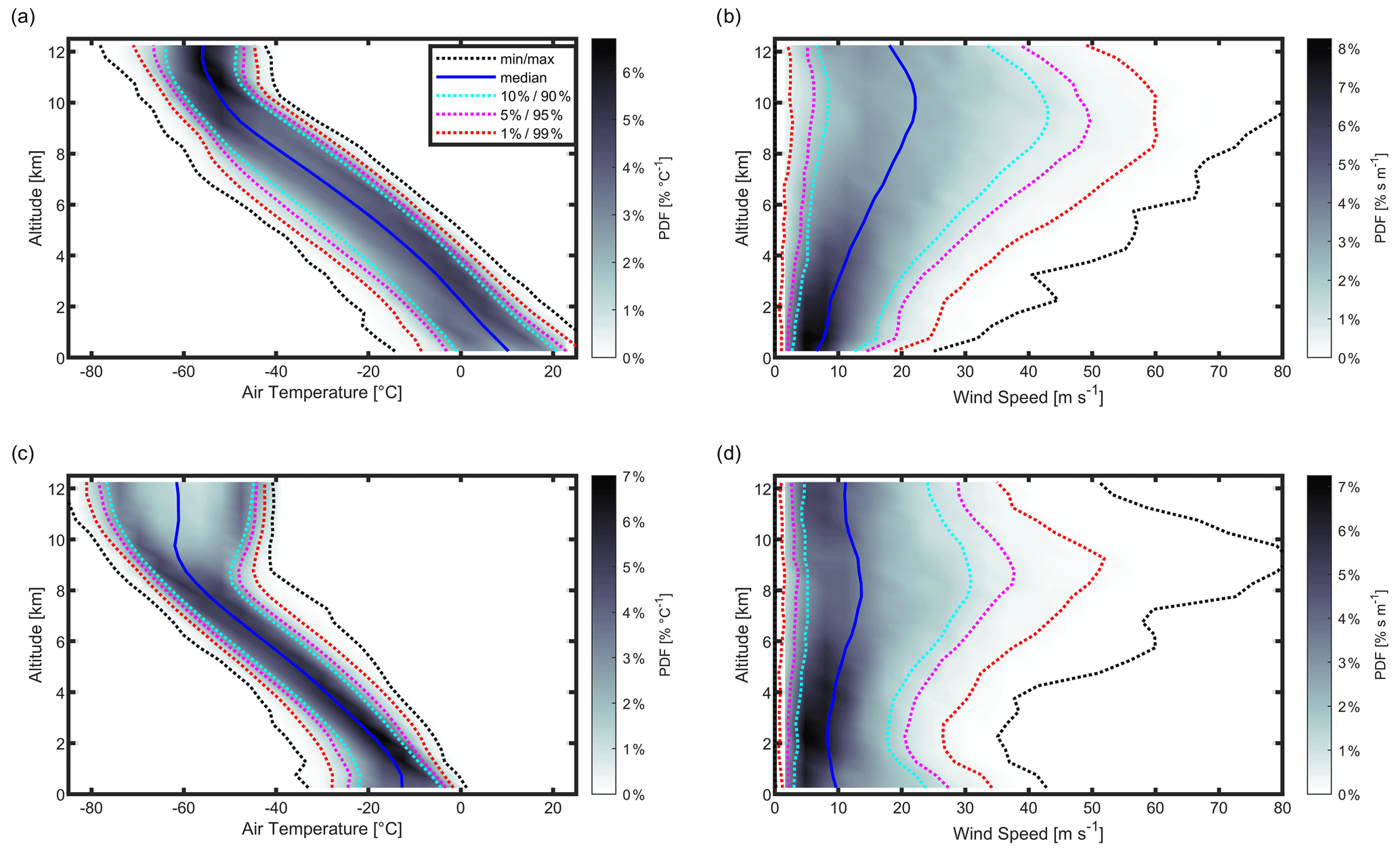
Figure 1Analysis of environmental constraints at the radiosonde stations Lindenberg in Germany (a, b) and Neumayer in the Antarctic (c, d). Panels (a) and (c) show the probability distribution function (PDF) of air temperature with altitude in greyscale and panels (b) and (d) the PDF of wind speed with altitude. The median is indicated in blue and the minimum and maximum values as dotted black lines, and the percentiles including 90 % (light blue), 95 % (magenta) and 99 % (red) of the data are indicated. The plot is based on the time period from 2016 to 2018, including all radiosonde launches at Neumayer around 12:00 UTC and all launches around 00:00 UTC as well as 12:00 UTC at Lindenberg.
In the following, the process towards the design of the LUCA-type drone is presented briefly. Requirements for the system are derived from the environmental conditions to be expected to obtain high availability of measurements. Based on the environmental conditions for two sites, the design of the mission and of the drone is introduced. The simplistic sensor package that was used for the demonstration flights is described, including uncertainty aspects. The process of obtaining flight permissions for such altitudes is presented. The methods for data post-processing are presented, and the data quality obtained is assessed. The section closes with a note on the variability of the atmosphere.
2.1 Environmental conditions
LUCA was designed to operate in mid-latitude and polar conditions. Therefore, the expected environmental constraints were evaluated from the radiosonde stations Neumayer in Antarctica and Lindenberg in Germany (Fig. 1) episodically over 3 years (2016–2018). The temperature range covering 90 % of the operating conditions of the ascents at Lindenberg is between −60 and 20 ∘C and at Neumayer is between −75 and −2 ∘C. For the Lindenberg station, the median wind speed is up to 20 m s−1, and the wind speed that is encountered in 90 % of the cases (90th percentile) is up to 42 m s−1 for the altitude of the jet stream (7–15 km) (Pena-Ortiz et al., 2013). For the Neumayer station, the median wind speed is up to 14 m s−1, and the wind speed that can be expected in 90 % of the cases is up to 28 m s−1.
Operational challenges at Neumayer arise from the surface wind speed, which is generally higher than in Europe. The most frequent surface wind conditions are either from the east due to cyclonic activities near the polar front, with a typical wind speed of 20 m s−1, or from the south due to katabatic flow, with a typical wind speed of 10 m s−1 (König-Langlo et al., 1998). High wind speed values are further reached at the altitude of the tropopause, around 9–13 km (Evtushevsky et al., 2008) in the polar jet stream (Archer and Caldeira, 2008).
The LUCA system was designed for operation in the temperature range between −75 and +30 ∘C and for a wind speed of less than 28 m s−1 over the whole vertical profile to limit the maximum vector displacement of the drone from its launch site. Assuming the system is capable of operating in conditions exceeding the design temperature and nominal wind speed by 15 %, this would allow ascents in 87 % of the radiosonde days at Neumayer in the Antarctic and 72 % at Lindenberg. Restricting wind speed conditions such that the drone does not have to stay above the launch point but must be able to return to the base, the mean wind speed over the atmospheric profile to be observed by the drone should not exceed the nominal horizontal airspeed component of 28 m s−1. Despite the limited applicability of this approach when using the drone in a reserved airspace and ignoring possible environmental threats such as heavy precipitation or in-flight icing, the system is capable of covering 94 % of the measurements in Lindenberg and 98 % at the Neumayer station. Adding a margin of 15 %, the availability increases to 97 % for Lindenberg and 100 % for Neumayer. At the Neumayer station, on 96 % of the days, radiosondes can typically be launched. Lindenberg has a temporal coverage of 99 % of all days. In addition, the development of the drone addresses measurements during rainfall, snow and heavy turbulence and within clouds, but these capabilities have yet to be proven in upcoming measurement campaigns.
Particular attention was paid to takeoff and landing under high-surface-wind conditions, which are accompanied at the Neumayer station by low visibility due to drifting and blowing snow. The probability of 23 % to operate under conditions with a visibility below 500 m requires a highly automated takeoff and landing procedure that does not rely on visual contact of the operator with the system, similarly to operations shown by Reineman et al. (2016).
A possible threat for drone measurements comprises in-flight icing conditions, which depend on temperature, humidity and droplet size (Jeck, 2002). An idea of the frequency of icing conditions might be available from icing forecast data using ADWICE (Advanced Diagnosis and Warning System for Aircraft Icing Environments; Tafferner et al., 2003) along with validation studies using PIREPs (pilot reports). Such comparisons exist for regions with dense air traffic, e.g. Europe (Kalinka et al., 2017), but no validation studies are found for the Antarctic. In addition, icing differs strongly between crewed aircraft (what ADWICE is made for) and drones (Hann, 2020). A report for Norway and its surrounding regions explicitly focused on icing for drones using meteorological reanalysis data (ECMWF ERA5; Hersbach et al., 2020) and an ice accretion model (ICE3D; Sørensen et al., 2021), and it found theoretical icing frequencies of 45 % at an altitude between 1–1.5 km between September and May and a lower risk with the highest frequency of 30 % peaking at 2.5 km altitude in June to August. These values are not directly applicable to the Antarctic, but the process to determine the likelihood of icing might be used to preliminarily estimate icing frequency and icing risk for drones in the Antarctic.
Drones are usually operated without sophisticated anti-icing and de-icing concepts like in crewed aviation, in particular as most drones are operated in visual line of sight. However, icing is a threat that may lead to a complete loss of the system. Icing protection for drones has been demonstrated (Hann et al., 2021) but requires additional substantial energy for heating, even if combined with specific ice-phobic coatings or liquids (Huang et al., 2019).
For the demonstration flights shown here, the LUCA drone was prepared to be equipped with an icing sensor to measure in situations with a substantial risk of meeting icing conditions during the flight, but the sensor was not installed during the demonstration flights as zero risk of icing was present. Together with monitoring performance parameters, this allows for estimating the severity of icing and supports the decision of abandoning the mission in icing cases. More details about the all-weather strategy can be found in Bärfuss et al. (2022).
2.2 System design
Before designing the physical aircraft system, the mission to be accomplished by the drone was defined. Although data assimilation is nowadays highly flexible regarding time, the mission was designed according to radiosonde observations to hypothetically surpass the 100 hPa surface at 12:00 UTC (Ingleby et al., 2022) and ensure timeliness in anticipation of future in-flight reporting analogue to radiosonde reporting, where a first dataset is sent to the GTS when the sonde reaches the 100 hPa level (Ingleby and Edwards, 2015). With a targeted climb rate of 10 m s−1 arbitrarily chosen from simple analytical estimates, the drone has to be launched around 11:33 UTC, and it reaches the design ceiling of 10 km at 11:50 UTC. During the flight, 1 Hz real-time data are available. After descending with a vertical rate similar to the climb rate, an approach procedure is flown in the vicinity of the landing site to determine wind direction and wind speed, and subsequently the approach trajectory is calculated automatically on the onboard computer. After the “splashdown” into a horizontal landing net, the drone can be recovered, and data processing including quality checks and transcoding begins. The observations of the complete flight are finally transferred into the GTS around 13:00 UTC. Thus, there is a target of making post-processed data from the descent profile available within an hour of the measurements being taken. Figure 2 illustrates the mission design.
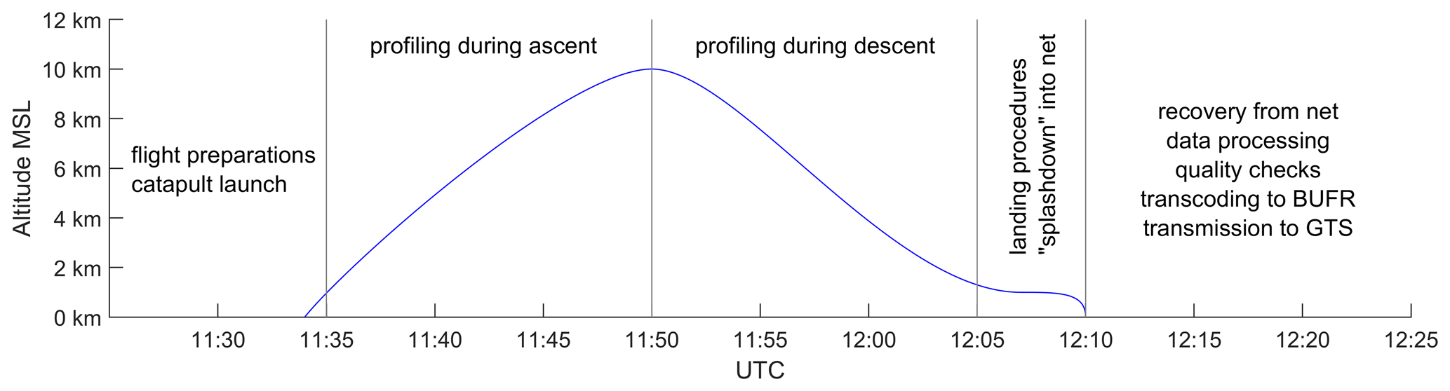
Figure 2Mission design for the LUCA drone. In order to be able to provide a first observation dataset for assimilation at 12:00 UTC, the drone is launched from the catapult at 11:33 UTC (as shown in Fig. 3a) and starts with the vertical sounding in the form of spirals at 11:35 UTC, hypothetically reaching the 100 hPa level at 12:00 UTC. After reaching its target altitude of 10 km at 11:50 UTC, the drone descends with a sink rate equal to the rate of climb (10 m s−1) until it arrives at the designated approach altitude around 12:05 UTC. After circles to determine the speed and direction of the near-surface wind, LUCA begins with the approach and lands in a horizontal landing net. Data processing, quality checks and transcoding into the WMO BUFR data format start directly after landing to enable data transfer of the complete flight to the GTS at around 13:00 UTC.
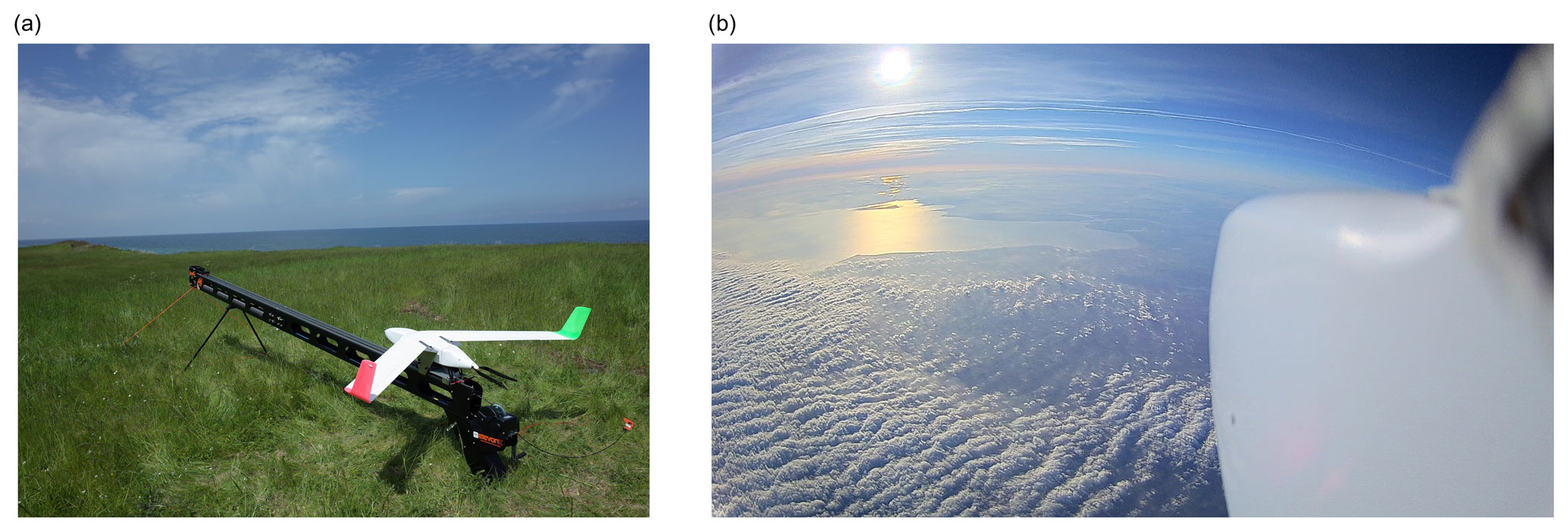
Figure 3(a) The LUCA drone mounted on the catapult to get airborne for measurements over the Baltic Sea. (b) A picture from the LUCA drone 10 km above the Lübeck Bight, the Baltic Sea, on 28 October 2021.
As key design driving parameters, the ability to fly against high-speed winds, an efficient electric propulsion chain and a highly flight-state-independent position for the sensor package are essential. These requirements led to the development of a tailless fixed-wing configuration with a pusher propeller. As the result of a multi-variant optimisation for profiling the atmosphere vertically up to 10 km, the design weighs 5–6 kg, depending on the deployed sensor package; has a wingspan of less than 2 m; and operates at a constant airspeed of 30 m s−1 with a typical ascent rate of 10 m s−1 controlled by the autopilot system. Thus, the system has a minimum airspeed of 18 m s−1, exceeding the minimum airspeed of crewed ultralight aircraft. Subsequently, it is not feasible to launch the drone by hand, and a dedicated mechanical catapult was adapted and used during the measurement campaign (Fig. 3a). As automatic takeoff and landing are required for future operations in zero-visibility conditions, a horizontal landing net has been developed and an appropriate manoeuvre to get the drone safely into the net was implemented in the autopilot firmware (ArduPilot). The manoeuvre itself can be considered an automated vertical dive into the horizontally arranged net. While a belly landing is principally possible, the net-landing technique was preferred as it protects the drone and the sensors from the hostile surface in the Antarctic, and prevents the system from being blown away and lost in low-visibility conditions of drifting and blowing snow in the case of high near-surface wind speed, as occurs frequently in the Antarctic. For the launch and retrieval system, no specific operation limits are in place regarding wind speed, as long as the launch and the landing is performed against the wind direction. Preliminary operating limits are therefore bound to the nominal airspeed of the drone. To address the risk of disintegration in turbulence, the airframe was constructed to resist gusts according to EASA Certification Specifications 23.333 (EASA, 2022). On the avionics side, the systems on the drone were widely predefined by national regulations (e.g. the redundancy of the command and control link). Bärfuss et al. (2022) reveal more technical details of the drone and its ground systems, which are not within the scope of this article.
2.3 Simplistic sensor package
An overview of the sensors and their accuracy according to the data sheet is provided in Table 1. The placement of the sensors is based on experience with similar drone-based systems (e.g. Bärfuss et al., 2018, 2021a; Lampert et al., 2020), and the sensor behaviour and possibilities of correcting, for example, sensor response time are well known. The performance of sensors and the data quality are assessed directly from the atmospheric measurements, without including wind tunnel tests for the overall setup.
To enable the autopilot sensors to measure dynamic and static pressure, a total pressure port (pitot tube) and static pressure ports on both sides of the drone were implemented in the nose section of LUCA. Below the pitot tube, an air inlet for the closed sensing path for the temperature–humidity probe (T/RH probe inlet) is installed, as sensor installation is known to influence the measurements (Jacob et al., 2018; Inoue and Sato, 2022). The combined resistance temperature and capacitive humidity sensor HMP110 (Vaisala, Finland), providing measurements of temperature and relative humidity in the closed sensing path, was mounted within the bulkhead, which separates the sensor chamber from the fuselage area. Subsequent to passing by the sensing elements, the air perfuses the measurement chamber and is vented out through apertures in the bottom of the nose section (venting). This ensures well-defined pressure conditions at the sensor location that are close to total pressure while maintaining ventilation of the sensing element. The ventilation rate, which is assumed to be still higher than the ventilation rate of radiosonde sensors, minimises the response time of the sensors as the sensor is exposed to an increased amount of air over time compared to radiosondes. The enclosure furthermore protects the sensors from damage due to ground contact, even during rough landings. An illustration of the sensor installation used for the measurement flights is provided in Fig. 4a, where the measurement nose of the drone is shown. As the body of the combined temperature and humidity probe is made of stainless steel and is mounted through the bulkhead between the sensor chamber and the fuselage area, thermal conduction into the sensor chamber which might affect the measurements is expected in the case of temperature differences between the ambient air temperature and the temperature inside the fuselage, as mentioned in, for example, Lampert et al. (2020). Additionally, the response times of the humidity measurements are expected to increase further, as the “wetted” area inside the sensor chamber is not well vented. Besides the sensors and pressure ports in the nose section, measurements of static and dynamic pressure, attitude angles, the Earth-related position, and velocities – all taken by the autopilot system (Cube Orange, HexAero, Singapore) – were recorded to derive atmospheric variables. As a drawback, the inertial navigation algorithm running on the autopilot system to calculate attitude angles, the Earth-related position and velocities relies on industrial-grade GNSS (global navigation satellite system), rotation rate, acceleration and magnetic field sensors, which limits the accuracy of the location and attitude estimation and subsequently limits the accuracy of the wind calculation, varying with the flight trajectory. Particularly, heading information might be adversely affected by electromagnetic interference originating from the power train, which is more pronounced during the ascent. Additionally, the estimation filter in the inertial navigation algorithm is not able to observe sensor (e.g. turn rate sensor) errors well during flight phases with low-trajectory dynamics. Measured parameters including data sheet uncertainties for both the LUCA drone and the radiosonde launched for data intercomparison are summarised in Table 1.
Table 1Sensor summary for the radiosonde and the LUCA drone using data sheet values.
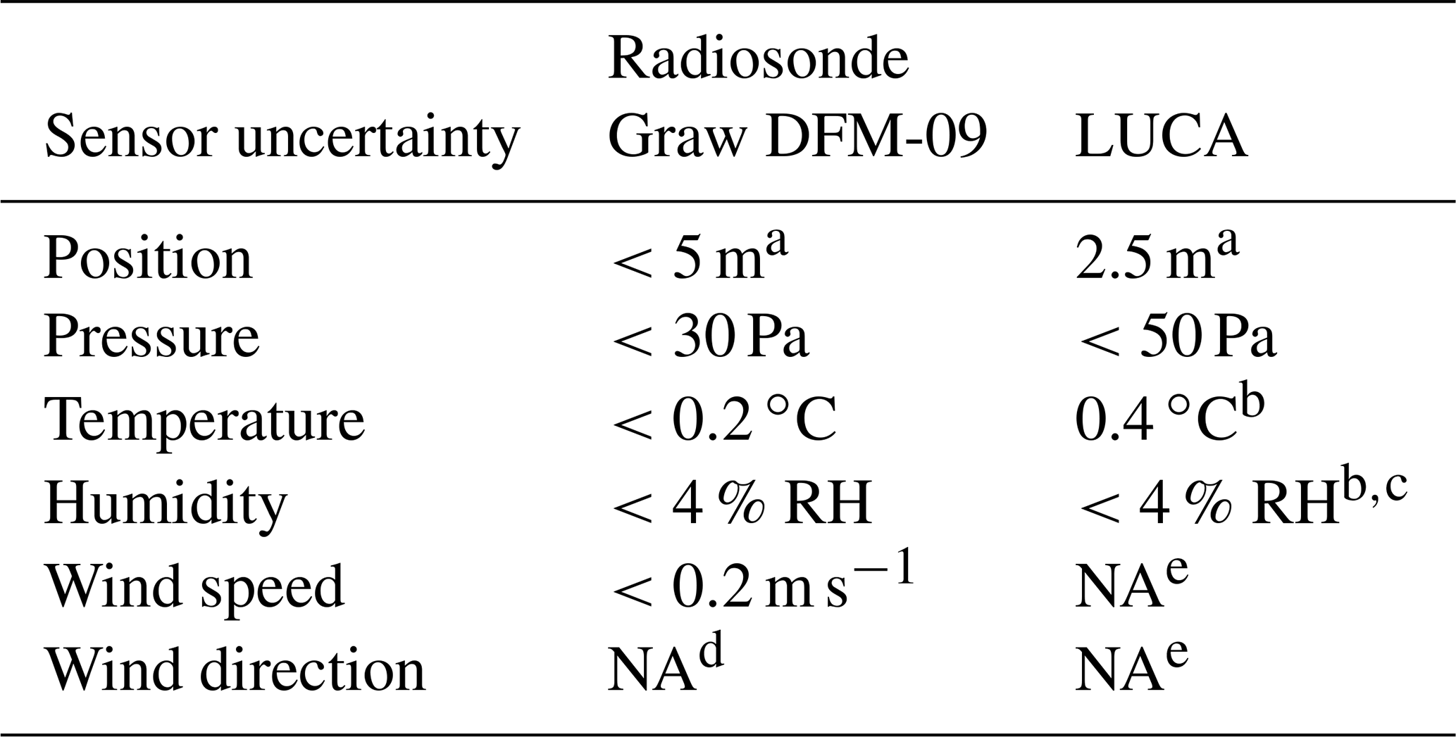
a Slightly differing between vertical and horizontal. b Data sheet measurement range from −40 to 80 ∘C. c Including non-linearity and repeatability. d Depending on wind speed. e Complex error behaviour. NA: not available.
As an example for a flight trajectory, the measurement flight on 28 October 2021 at 07:20 UTC is shown in Fig. 4b. The trajectory during the measurement flight consists mainly of circular patterns and therefore provides trajectory dynamics to facilitate the calculation of aircraft attitude, velocity and position performed by the inertial navigation algorithm.
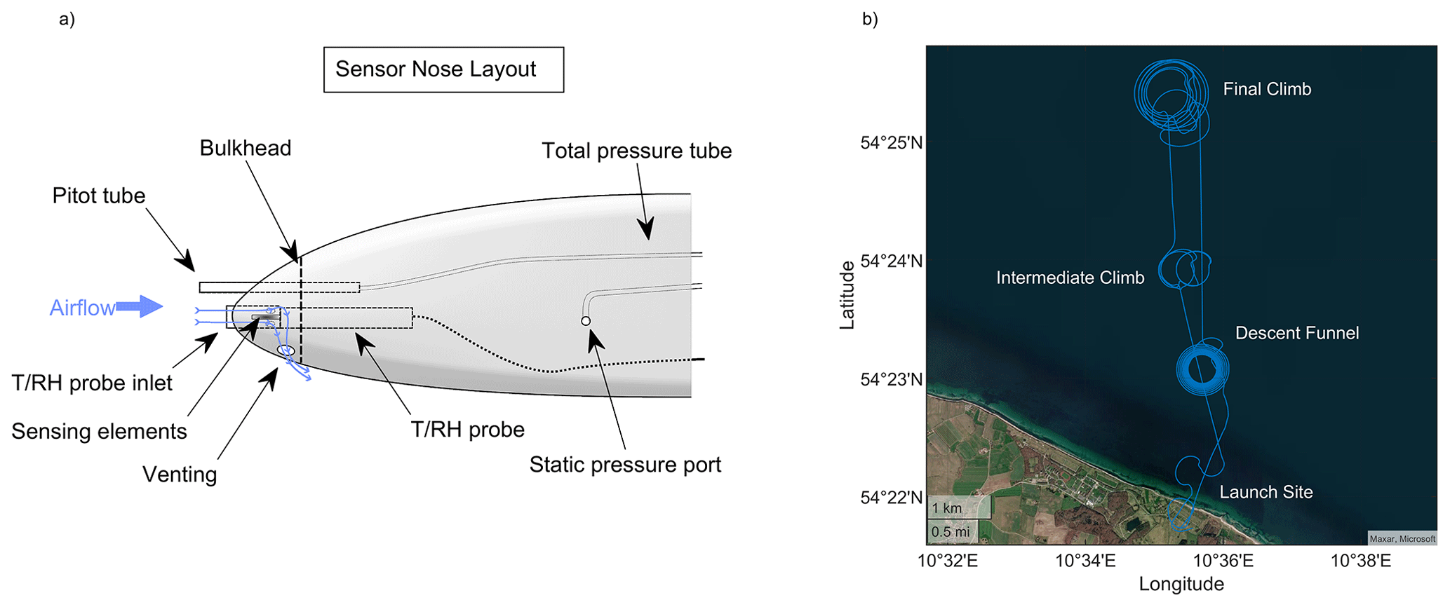
Figure 4(a) The measurement nose section with pressure ports for total pressure (“Pitot tube”) and static pressure (“Static pressure port”) and the installation of the temperature and humidity probe (“T/RH probe”, HMP110, Vaisala, Finland). The probe itself is mounted in the bulkhead, which separates the sensor chamber from the general fuselage area. The air enters the air inlet (“T/RH probe inlet”), passes the sensing element and is vented out through apertures in the bottom of the nose section (“Venting”). (b) Trajectory of the measurement flight on 28 October 2021 at 07:20 UTC – besides the launch site, the intermediate climb position where the drone climbs up to 3 km and the final climb position where it climbs up to ceiling, as well as the descent funnel, are labelled.
A cut-out in the left wing is foreseen to be used for an icing sensor as shown in Bärfuss et al. (2022), but other instruments can be fitted into it. As the risk of in-flight icing was negligible during the measurements, a camera was installed into the cut-out. The camera captured video and audio during the measurements, see Fig. 3b, and helped to analyse the behaviour of the flight controller and the motor controller of the drone.
2.4 Permissions for operation
The most important aspects for drone flights relate to safety. Operational requirements are different for each region of the world; however, in Europe, there are now unified regulations for drone operation (EASA, 2022). The requirements concerning redundancy and the level of integrity of the drone depend on the overall risk analysis. For relatively small and lightweight drones performing flights beyond visual line of sight, which is the case for any system operating up to an altitude of 10 km, the drone falls into the category “specific”, and precautions to avoid damage to a third party have to be met. An operational handbook includes, for example, regular checks and maintenance of vital parts like motors and propellers, redundancy in the electric system, regular training of the crew, independent control links, and many more aspects defined in the so-called operational safety objectives. The flight tests were therefore done in restricted military areas, in this case close to the Baltic Sea, Germany, and the internationally recognised high-quality portable radiosonde system of Graw, Germany (Nash et al., 2011), was deployed from the launching site for direct comparison. In the restricted areas, cooperation with the German Federal Armed Forces is required, and flight permission of the German Federal Supervisory Authority for Air Navigation Services (Bundesaufsichtsamt für Flugsicherung, BAF) is necessary.
For the operation in the Antarctic, a thorough risk assessment was performed with particular emphasis on safety and redundancy to avoid damage to third parties even in such a sparsely populated area. Further, for the deployment in the Antarctic, permission of the German Environmental Agency (Umweltbundesamt) is required, ensuring that no material stays in the pristine environment and that the penguin population near the Neumayer station is not disturbed.
2.5 Method to assess the data quality of the simplistic sensor setup
For a comparison of data obtained by LUCA and radiosonde data, a procedure similar to what is presented in Wagner and Petersen (2021) is applied to the data. In a first step, data within pressure bands of 2 hPa are found for drone observations and radiosonde observations. Assuming a constant wind situation at the particular altitude associated with the pressure band, the air parcel measured by the radiosonde is shifted with the wind according to the time difference between the drone measurement and the radiosonde measurement. For example, if the drone was measuring at 09:20 UTC within the pressure level of 500 hPa and the radiosonde was measuring at 09:30 UTC at the same pressure level, the radiosonde position would be shifted backwards by the distance an air parcel would have been travelling within this 10 min period in constant wind at this particular pressure level. This leads to a “source” position of the air parcel measured by the radiosonde at a specific time – the time when the drone was measuring at the same pressure level (altitude). These virtual positions are then taken into account to select measurements collocated in space and time. Collocation conditions identical to the conditions used in Wagner and Petersen (2021) (spatial distance less than 50 km, temporal gap less than 30 min) were then applied, before measurements were intercompared. No explicit filter for outliers was applied, but the drone data were implicitly filtered for outliers by median-filtering the data measured in each particular pressure band of 5 hPa width. Differences were computed for all pressure bands on all six flights.
In the following section, the technical achievements and the resulting potential of drone measurements are presented. Therefore, the data are discussed in a qualitative and a quantitative way.
3.1 Technical achievement: first flight up to 10 km with a battery-powered meteorological drone
LUCA represents a new type of small fixed-wing drone. The combination of a relatively small wingspan below 2 m and a total weight of more than 6 kg leads to a high minimum flight speed of 18 m s−1 at sea level for obtaining the lift required to fly and therefore complicates the process of getting airborne and landing safely compared to aircraft with larger wing areas related to the total mass. During the flight test and measurement campaign, the design altitude of 10 km was reached. Ascending to such altitudes can be regarded as unique for an electrically powered fixed-wing drone without solar panels. To the authors' knowledge, it is the first time that a meteorological drone powered only by electrical batteries reached the altitude of 10 km. In addition, the landing manoeuvre has been proven to be repeatable during test flights without manual control. A list of flights performed can be accessed in Bärfuss et al. (2022). During flight tests at sea level, a maximum airspeed of more than 60 m s−1 was reached, indicating that the drone is able to operate in equally high wind speed (Pinto et al., 2021). For operations, a safety margin has been applied, and the designated horizontal wind speed limit for normal operations was set to 28 m s−1, which equals the nominal horizontal component of the true airspeed during the ascent. Drifting away from the measurement location is prevented by forcing the minimum ground speed to 2 m s−1. The flight controller automatically increases the airspeed when the minimum ground speed falls below the threshold because of high wind speed – potentially trading the climb rate for airspeed. Resisting high wind speed and the corresponding turbulence was demonstrated during the flight on 25 October 2021 starting at 12:12 UTC, where the maximum measured wind speed was 28 m s−1 during ascent and descent at an altitude of 7800 m a.m.s.l. (above mean sea level). Operations in BVLOS (beyond visual line of sight) conditions and in the presence of closed cloud layers have been conducted successfully.
The drone measurements can take place starting from any location, up to the altitude of 10 km, if flight permission is obtained. Operations are completely independent of additional infrastructure, like an airport, or the availability of helium. The drone only requires a cylindrical airspace with a radius of about 11 km for the whole mission. The drone ascends and descends at a vertical speed of 10 m s−1 and a horizontal speed component of 100 km h−1. Therefore, the mission reaching up to 10 km altitude and returning to the landing site takes in total 33 min. The data are available by remote transfer with a temporal resolution of 1 Hz. The full dataset with a resolution of up to 25 Hz can be downloaded after landing and is preprocessed automatically for upload into the GTS. The subsequent launch after landing can be typically performed after a turnaround time of 20 min.
3.2 Qualitative comparison of meteorological observations between drone and radiosonde data
A measurement campaign with LUCA and radiosondes was performed over the Baltic Sea (54.4∘ N, 10.6∘ E) from 25 to 29 October 2021. An overview of the development of the meteorological conditions with altitude is shown in Fig. 5, based on hourly ERA5 reanalysis data (Hersbach et al., 2023, 2020). The distribution of relative humidity with time and altitude was highly variable during the measurement period. Also, wind speed and wind direction (indicated with wind barbs) varied with height and time. The temporal distribution of the LUCA flights and parallel additional radiosondes are indicated in the overview (Fig. 5). LUCA was tested during a time period with high relative humidity, corresponding to cloudy conditions, and with high wind speed of up to 50 m s−1, but the drone was not operated at the time of the maximum wind speed at 9 km altitude. The overall wind direction was from the west with surface wind speed around 10 m s−1 and an absence of precipitation. Low and high scattered cloud layers were present, and a broad jet stream was forecasted just in the north of Denmark, with the jet core expected at 400 km distance to the north of the measurement campaign location.
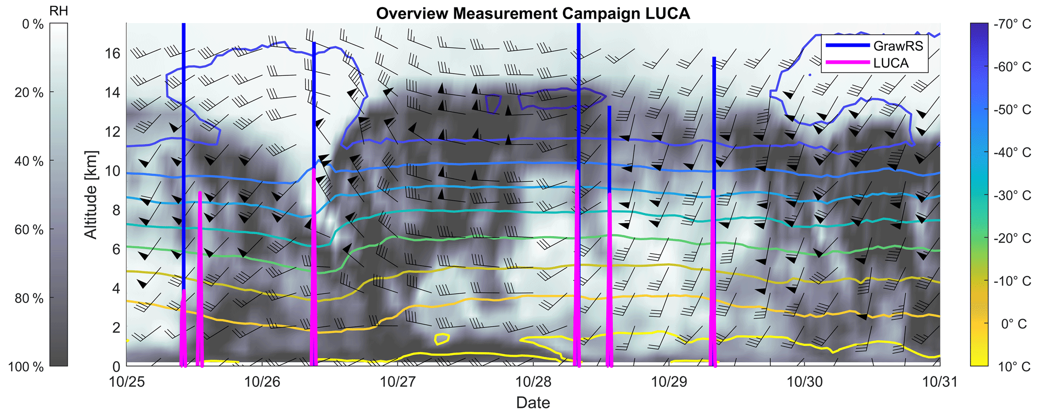
Figure 5Overview of the meteorological situation between 25 and 31 October 2021 (date format: month-day) using ERA5 reanalysis data at the grid point closest to the drone measurements. The background in grey indicates relative humidity (linearly interpolated between times and levels), whereas the coloured isolines indicate air temperature. The measurement times using the LUCA drone are shown in magenta; the measurements with a timely and spatially collocated radiosonde (type DFM-09, Graw, Germany) for comparison with the drone data are marked in blue. The wind barbs as defined in WMO (2011) indicate the high wind speed during the measurements, which coincides with the high variability in humidity over time.
Exemplarily, Fig. 6 shows measurements of temperature, relative humidity, wind speed and wind direction recorded by LUCA at up to 10 km. The measurements took place on 26 October 2021 at 08:45 UTC and on 29 October 2021 at 07:22 UTC. The data of the nearly simultaneous radiosonde are shown, as well as ERA5 reanalysis data.
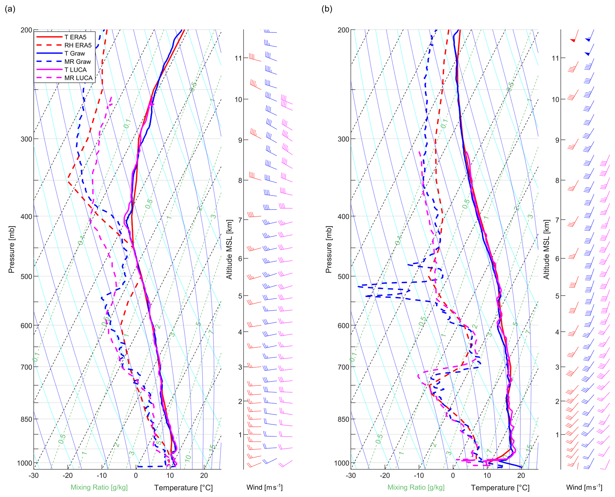
Figure 6Skew-T log-p diagrams of the vertical profiles (descent) of temperature (solid lines), dew point temperature (dashed lines) and wind (wind barbs) measured with LUCA data in magenta, the simultaneously launched radiosonde data in blue and ERA5 data in red. In (a), the launch time of LUCA was 08:45 UTC on 26 October 2021 and the radiosonde was released at 09:11 UTC. The drone profile was measured during the descent from 09:09 to 09:30 UTC. In (b), the drone was launched at 07:22 UTC on 29 October 2021 and the corresponding radiosonde was released at 08:01 UTC. The drone profile was measured during the descent from 07:47 to 08:12 UTC. Statistics as well as observation uncertainties are shown in Fig. 8 for the profile presented in panel (b).
Each profile provided by LUCA shows qualitatively the same atmospheric structures as the radiosonde measurements with a similar sensor package to that used on the radiosondes.
On 26 October 2021, the strong temperature inversion at 400 m as well as the transition to a different temperature gradient at an altitude of around 6500 m is equally captured by the drone and the radiosonde measurements (Fig. 6a). On 29 October 2021, the temperature inversion at the top of the boundary layer at 400 m altitude is captured by the drone and the radiosonde, as well as ERA5 analyses.
Humidity was generally moderately variable during the observation period. The drone and radiosonde measurements, as well as ERA5 data, agree that there was high relative humidity (small differences between dew point temperature and temperature) up to the temperature inversion at around 400 m altitude on 26 October 2021 (Fig. 6a). On both days, there were layers of lower and higher humidity. On 26 October 2021, in the lower troposphere up to an altitude of around 4 km, the individual layers of different humidities are identically resolved by the drone in terms of altitude and magnitude (Fig. 6a). On 29 October 2021, humidity measurements using the drone are in good agreement with radiosonde data up to 500 hPa (around 5 km altitude, Fig. 6b). Above 500 hPa, an increasing deviation between radiosonde and drone measurements can be observed in humidity for both days. This is likely caused by the dramatically increasing response time of the humidity sensor at lower temperatures (Choi et al., 2018; Majewski, 2020) in addition to the delaying effect of the implemented closed-path sensor setup. Moisture is a critical parameter to measure in the upper troposphere (Nash et al., 2011; Dupont et al., 2020).
Wind measurements agree well between the drone and the radiosonde measurements. When comparing the measurements directly, one has to take into account that the radiosonde was launched 53 min after the drone. A systematic deviation can be expected for higher altitudes due to the drifting of the radiosonde with the wind, towards the north-east, which resulted in a spatial distance of 40 km from the launch point when reaching the altitude of 10 km.
3.3 Case study: quantitative intercomparison of the simplistic sensor setup and radiosonde data
Despite the simplistic sensor setup, data measured on board the platform LUCA have been shown to compare at least qualitatively with radiosonde data. To assess quantitative measures, the methods presented in Sect. 2.5 are applied to the data of all six vertical profiles (upwards and downwards) post-processed according to Appendix A. These techniques were applied for ascents as well as descents, as data during the ascent are expected to suffer from electromagnetic interference as well as other factors such as thrust line misalignment. The collocated dataset for the pressure bands of 2 hPa width from 1000 to 250 hPa consists of 694 data points for the ascent and 1323 data points for the descent of the drone. Figure 7 shows histograms of the differences between the radiosonde observations and the drone observations for the variables temperature, relative humidity, specific humidity, wind speed, wind direction as well as the norm of the wind vector difference for the descending profiles. Within the histograms, average differences as well as the standard deviation of the intercompared observations are provided.
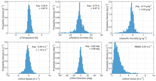
Figure 7Histograms (probability density over observation difference) of the differences between collocated LUCA drone and radiosonde observations for various atmospheric variables. Collocation was assumed for the probed air parcels' virtual spatial distance of less than 50 km and an observation time difference of less than 30 min. The virtual air parcel position was determined by virtually back-shifting the probed air parcel with the negative mean wind vector at the observation level multiplied with the time difference between the drone and the radiosonde measurements within the same pressure level band. All histograms suffer from the sparse database but indicate a Gaussian-like distribution of observation differences, except the difference in the wind vectors, which follows a Rayleigh distribution as expected from theory. Therefore, the root-mean-square deviation (RMSD) is shown in the histogram for the wind vector difference rather than standard deviation as for the other parameters.
Despite the sparse database consisting of six vertical descent profiles, the distributions of the differences for the variables of temperature, relative humidity, specific humidity, wind speed and wind direction are similar to Gaussian distributions. The histogram for the norm of the wind vector difference follows a Rayleigh distribution, as is expected for the norm of a two-dimensional vector whose components are stochastically independent Gaussian processes. For the distribution of the observation differences, the average deviation and the standard deviation (root-mean-square deviation for the Rayleigh distribution) were calculated and are shown in the histogram plots (Fig. 7). These values were retrieved for both the ascent and the descent and are shown in Table 2.
Table 2Statistical measures for the differences in the collocated observation of temperature, humidity and wind between drone measurements and radiosonde measurements. Collocation was assumed when an air parcel, virtually reverse-shifted by the mean wind and the time difference, was within a spatial distance of 50 km and a temporal difference of 30 min. The statistical measures are shown for both the descent and the ascent profile compared to radiosonde data. During the six ascent profiles, an increased variation in wind observations, particularly the wind direction, can be found compared to the six descent profiles.
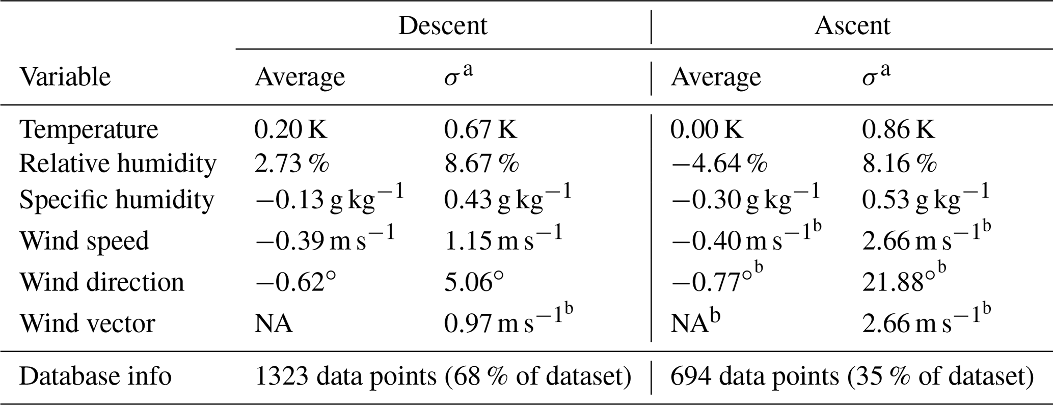
a RMSD for the wind vector difference. b Wind observations during ascent are regarded as invalid due to electromagnetic interferences. NA: not available.
Comparing the statistical measures between ascent and descent data, increased differences between the radiosonde and the drone observations are revealed. This is most likely associated with a magnetic deterioration or a possibly induced sideslip angle when the thrust line is not aligned with the drone's body (see Sect. 2.3 and Appendix A3). For the descent profile, the average differences as well as the standard deviation of the differences between drone observations and radiosonde observations are in the range of (or even below) statistical measures shown in the study of Wagner and Petersen (2021), which includes a comparison of radiosonde data with observation data from the AMDAR–TAMDAR programme. The statistics furthermore support the values of the theoretical error estimation in Appendix C. For the humidity measurement, the average of the differences between radiosonde and LUCA measurements differs significantly between ascent and descent, indicating the possible need for further calibration and tuning of the post-processing parameters using a broader database in the future.
The overall uncertainties for the measured profile in Fig. 6b are shown in Fig. 8. As the contribution of the time lag correction and the wind calculation to the total uncertainty depends on the vertical profile itself, the total uncertainty for the variables of air temperature, relative humidity, wind speed and wind direction is shown as a grey area around the measurements.
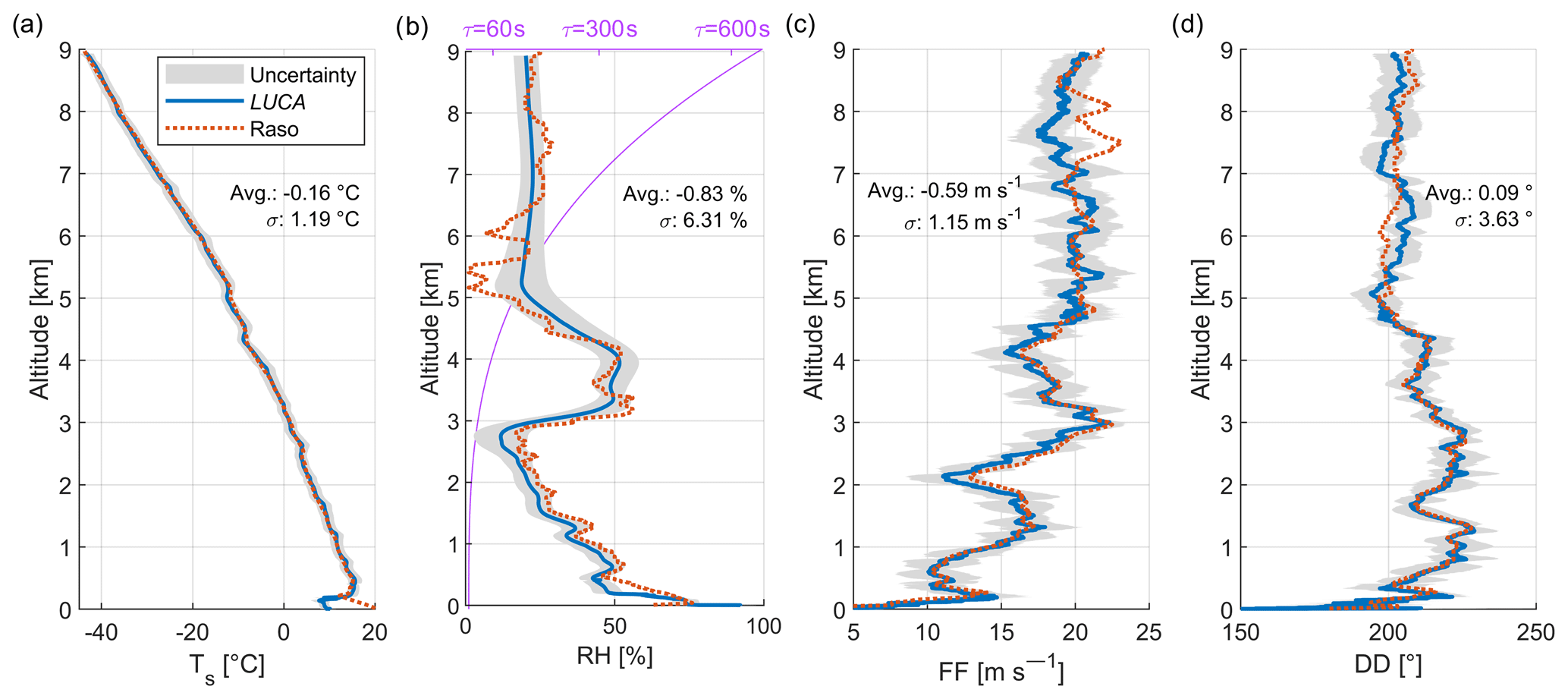
Figure 8Measurements and associated uncertainties in the LUCA drone during the descent on 29 October 2021 from 07:47 to 08:12 UTC and the radiosonde (“Raso”) launched on the same day at 07:22 UTC, i.e. the same measurements as shown in Fig. 6b. For the vertical profiles of static air temperature Ts in (a), relative humidity RH in (b), wind speed FF in (c) and wind direction DD in (d), the corresponding radiosonde profile is plotted. The grey areas surrounding the profiles depict the estimated uncertainties in the measured variables according to Appendix C. Intercomparison statistics for the profile are added in each of the panels. The time constant for the smoothing filter for the temperature in (a) is 4.2 s (roughly comparable to centred average smoothing across 120 m altitude), whereas the lilac curve in (b) indicates the variable “time constant” τ (≠ time span) for the phase-neutral smoothing filter applied to the humidity measurements, for which no accessible replacement value for a centred average exists.
For the air temperature Ts in Fig. 8a, the radiosonde observations deviate significantly in the lower boundary layer, likely caused by the temperature sensor being heated up by solar irradiance without venting on the ground before the launch. No particular uncertainty source dominates the total uncertainty for the measurements. For humidity observations in Fig. 8b, increased uncertainty around rapid changes in humidity is visible, originating in the uncertainty caused by the time lag correction. The data sheet uncertainty dominates the total uncertainty, in which the calibration drift (up to ±2 % per year according to the data sheet) is not yet included. Radiosonde observations lie partly outside the uncertainty area (1σ plus systematic errors) for the drone measurements, potentially pointing to the need for further measurements and investigations. Wind observations in Fig. 8c and d compared to the radiosonde measurements are within reason regarding the uncertainty and taking into account turbulence as well as the spatio-temporal distance between the radiosonde and the drone.
The in situ data gap in the Global Observing System was reviewed in the Introduction. Experiments on the impact of additional vertical profiles on NWP suggest that in situ observations of the complete tropospheric column in remote areas improve forecast quality, which more frequent sampling of the atmosphere also would. Besides the effort in filling the observation gap in the near-surface boundary layer with drones (Leuenberger et al., 2020; Pinto et al., 2021; Inoue and Sato, 2022), the data gap with drone measurements in the free troposphere and the lower stratosphere has not been addressed – the technology of small drones has not been ready for observations at such high altitudes (Geerts et al., 2018; Pinto et al., 2021).
The drone measurements presented here show the potential for covering data gaps as the drone has the capability of measuring frequently, e.g. hourly, with moderate cost and effort. More frequent observations increase the forecast quality (Dabberdt et al., 2005; Faccani et al., 2009), as special atmospheric features like the diurnal cycle can be resolved. The required frequency of measurements strongly depends on the temporal variability of the atmosphere, which is highly variable for different altitude ranges and different for each meteorological parameter, as shown in Fig. D1. The atmospheric boundary layer experiences high temporal changes in temperature, wind speed and humidity. Besides these diurnal variations in the lowermost region, temporal changes in temperature and wind speed are seen in the upper troposphere and the lower stratosphere. Processes in this layer ± 5 km around the tropopause (the virtual boundary between the troposphere and the stratosphere, e.g. Gettelman et al., 2011) are known as being important for global (mass) exchange (Holton et al., 1995). Humidity, in contrast, varies highly from the ground up to the lower stratosphere with no preference in terms of timescales, representing a chaotic system. Interestingly, temperature variability at six cycles per day is low below 5 km altitude (besides the high variability in the boundary layer), emphasising the importance of profiling the atmosphere to higher altitudes. In NWP, physical processes are modelled to predict a future atmospheric state. The modelling of these processes performs quite well on distinct timescales to reproduce the variability of the atmosphere. The need for observations therefore not only can be defined by the atmospheric variability to avoid undersampling, but also has to be seen as complementary to the stability of the modelled physical processes and regional data gaps. Specified by data users, the WMO provides data requirements for observation spacing and uncertainty (WMO OSCAR, 2015; Leuenberger et al., 2020), which interestingly differ only little between the boundary layer and the free troposphere for both global and high-resolution NWP, emphasising the benefits of profiling the atmosphere vertically with a drone up to approximately 10 km and above. Filling the in situ observation gap in both the atmospheric boundary layer and the free troposphere will result in better forecast quality and even has the potential to further adjust and develop the modelling of the underlying physical processes.
This article presents atmospheric soundings up to 10 km altitude using an electrically powered fixed-wing drone. The developed system represents a milestone, demonstrating the capability of fixed-wing drones to perform tropospheric soundings. Measurements with a basic atmospheric sensor package were conducted. The drone measurements of temperature, humidity and wind reported here generally agree with temporally and spatially coinciding radiosonde measurements. Minor drawbacks in the measurements occurred as expected due to the simple sensor setup.
Moisture is generally the most challenging parameter of in-flight atmospheric observations, which demands significant post-processing. This is also a known issue for standard radiosonde systems, where various corrections need to be applied as well (Dirksen et al., 2014). By design, the drone technology bears the pivotal advantages of re-using sensors and the possibility of pre- and post-flight calibration.
More advanced sensor techniques that are available could be integrated into the platform. This would enable us to extend the measured parameters or focus on high-quality measurements of basic atmospheric parameters, e.g. by using dew point mirrors for humidity (Fujiwara et al., 2003) or fine wire temperature sensors with suitable shielding and protection (Stickney et al., 1994; Bärfuss et al., 2018). As an outlook, standard radiosonde accuracy is expected to be reached or even surpassed using a more sophisticated measurement package instead of the simplistic sensor integration used within this study. Sensor limitations and challenges are known; the needs regarding data management (Wyngaard et al., 2019) are not addressed within this article.
The LUCA system was designed to reach its target altitude (10 km) in conditions with average wind speeds of up to 28 m s−1, which results in a minimum flight speed of 18 m s−1. The limitations concerning wind speed are related to the current maximum airspeed of 50 m s−1. In order to ensure the aforementioned operability, LUCA was constructed with suitable ground systems for takeoff and landing. The mechanical start catapult enables robust starts, even in challenging conditions of high wind speed and virtually zero horizontal visibility. The landing net was designed for an automated landing manoeuvre, which allows for landings during high-surface-wind and low-visibility conditions.
As for now, LUCA does not incorporate measures to actually prevent icing but features a dedicated sensor to detect icing. This enables safe operation of flights but limits operability significantly. In future developments, this issue needs further attention.
The reported flights that were carried out demonstrate the general suitability of the technology for the envisaged purpose, explicitly covering rather challenging environmental conditions. However, systematic and extensive tests in adverse weather still need to be performed in the future. Nevertheless, the LUCA system was successfully operated above the design wind speed and through closed cloud layers.
Data quality assessed within a case study using a simple sensor package indicates observation accuracy comparable to AMDAR and TAMDAR observations, but further studies have to be carried out, as the observations within the case study cover only limited atmospheric conditions.
Receiving permissions for drone operations beyond visual line of sight is a demanding prerequisite for atmospheric measurement systems like LUCA. With its design mass of 5–6 kg, LUCA is fairly light compared to crewed aircraft but significantly heavier than typical radiosondes. Hence, the operational risk is an issue. By further miniaturisation of the system, both air and ground risk can be reduced and hence is expected to simplify the process of granting permissions.
Compared to existing in situ observing systems, the vertical profiles are similar to radiosonde ascents and descents (in some NWP centres, radiosonde descents have already been assimilated; Ingleby et al., 2022) and aircraft-based observations close to airports. The assimilation of drone data into the BUFR format (Ingleby and Edwards, 2015; Ingleby et al., 2022) should therefore be quite straightforward compared to new and complex assimilation processes of, for example, radio occultation data (Eyre, 2008). In comparison with observations from crewed aircraft, drones typically operate at a lower airspeed, which tends to result in an increased wind observation accuracy (Pätzold, 2018). Even though reaching 10 km can never replace the well-established radiosonde network, the system has the chance to augment radio soundings with more frequent drone measurements. Furthermore, in the future, it might be feasible to set up atmospheric in situ monitoring programmes by combining profiling drones such as the one presented here with solar-powered semi-permanent systems in the stratosphere.
There are several possible applications and opportunities for the use of small drones measuring the complete tropospheric column and potentially the lower stratosphere – sampling the atmosphere with an increased number of observations per day with re-usable individual sensors has to be highlighted here. Re-using sensors inevitably leads to substantial knowledge about the stability, strengths and flaws of an individual sensor and has the chance of increasing the ability to precisely specify the uncertainty in observations, which is substantial for data assimilation. This effect is regularly observed regarding satellite sensor assessments (Rennie et al., 2021).
The use of reference radiosondes to characterise the uncertainty in NWP models to improve satellite validation and calibration is another future application (Carminati et al., 2019) to which drone measurements potentially can contribute. The quality of drone observations for sampling the complete troposphere is of superior importance and could possibly contribute to climate applications. Regarding the variables involved, one finds that climate users tend to focus on temperature and humidity data (Ingleby et al., 2022).
For NWP applications, wind observations have arguably more than twice the impact on the quality of short-range forecasts compared to temperature observations (Ingleby et al., 2021). In order to augment and compete with the well-established vertical profile observations (radiosondes, airliner-borne) and be used operationally, a drone must be operable by station staff of existing atmospheric observatories. Furthermore, the system needs to cope with a variety of challenging environmental conditions, including high wind speed, poor surface visibility or icing during the flight.
Upcoming implementations of such systems in the GTS will likely depend on investment cost as well as cost generated by the effort for station staff in respect to operations and maintenance. A generic approach to assessing the economical benefit for drone-based observations is presented in Bärfuss et al. (2022), but acquisition and operational costs are widely unclear for the system presented here, in particular regarding system failures and hardware issues.
Targeted observations were discussed controversially, as their impact strongly depends on the assimilation scheme and the NWP system (Schindler et al., 2020). Unquestionable are the use of drone measurements in contributing to scientific campaigns and the resulting reduction in cost and waste when used to replace frequent radio soundings during intense observation periods.
Although this study demonstrates the feasibility of using small drones up to the troposphere as carrier systems for atmospheric observations, envisaged extensive test campaigns (like the WMO UAS Demonstration Campaign; WMO, 2022) are needed to assess the impact of drones on forecast skills and will increase and demonstrate the reliability of LUCA in performing successful and safe tropospheric profiling.
As a fundamental principle, every sensor reading a physical quantity involves a transfer function G(s) from the physical quantity to the sensing element. A transfer function, utilising techniques from the field of control theory, can be noted in the complex frequency domain as
with the input signal X(s), the output signal Y(s) and the complex frequency domain parameter s. Besides the trivial proportional transfer function H(s)=P, which denotes , a common transfer function describing physical processes is the first-order lag function:
where τ is the so-called time constant. In the time domain, such a system has an output rate of change proportional to the difference between the input x and the output y, scaled with the time constant .
An example of a sensor with an inherent first-order lag transfer function is a thermistor air temperature sensor, where the heat transfer between the sensor head and the ambient air drives the rate of temperature change of the sensor head and therefore the temperature readings.
A1 Temperature corrections
The temperature sensor head on board the drone presented here is a thermistor element of specification Pt1000. This type of sensor naturally involves a non-uniform time lag represented by a first-order lag transfer function. This implies spectral errors and an input-signal-dependent time lag in the temperature time series, which are in theory fully recovered using the signal reconstruction (also called inverse filtering) method. The basic idea is to apply the inverted transfer function to the measured sensor output, taking advantage of a priori knowledge during the post-processing.
Expressed by a linear differential equation, the measurement process for the thermistor sensor is defined with
where the quantity to measure is denoted by x, the measurement by y (both as a function of time t) and a time constant by τ. is the derivative of y(t) with respect to the time t. Assuming a step change on the input side and solving the differential equation, the time constant represents the sensor response time in the way that the measurement will reach 63 % of the input state within the time span τ. Having identified the time constant for the sensor response, the signal reconstruction of the measurement time series y(t) can be applied to determine the quantity to measure x(t) by applying Eq. (A3). As the derivative of the measurements is needed for signal reconstruction, measurement noise will be amplified in the recovered signal and is phase-neutrally low-pass-filtered by filtering the recovered signal forwards and backwards (e.g. Bärfuss et al., 2018).
The spectrally corrected temperature measurements then represent the actual temperature at the stagnation point at the sensor position. In aviation, this is called “total air temperature” Tt and can be transferred into the static air temperature Ts, i.e. the temperature of the undisturbed air around the aircraft, with
where k≈1.4 is the adiabatic index of air and Ma the Mach number. The temperature difference between Tt and Ts is caused by energy conversion from kinetic to thermal energy in the air, but as the air at the sensed area with the temperature Traw is not subject to a complete adiabatic process, an additional recovery factor in the range of about 0.6–0.95 has to be applied to the temperature rise Traw−Ts when using Eq. (A4) (e.g. Lenschow, 1972; Bange et al., 2013).
The aforementioned correction for the temperature rise is not applied to the measurements presented here, as the error is expected to be small.
An error correction rather specific to the sensor installation in the LUCA drone is the correction for heat transfer through the metal sensor housing between the fuselage area and the sensor chamber, as is visible in the sensor package sketch in Fig. 4a. The corrected temperature Tc can be assumed to behave as
with the recovered temperature signal Tr, the temperature Tf measured inside the fuselage and a dimensionless coefficient m for the magnitude of the heat transfer. The coefficient m, which expresses the heat transfer rate from the fuselage to the sensor, is regarded as independent of environmental conditions and universal for all temperature measurements with the drone LUCA.
A2 Humidity corrections
Similarly to resistive temperature measurements, capacitive moisture measurements suffer from a time lag which can be described by using a first-order lag transfer function (Miloshevich et al., 2004; Dirksen et al., 2014; Bärfuss et al., 2018; VAISALA, 2021). In contrast to temperature sensor transfer functions, the time constant of humidity observations is heavily affected by the ambient temperature, as the diffusion process acting on the sensing element is slowed down in low temperatures (e.g. Miloshevich et al., 2004; Choi et al., 2018; Majewski, 2020). The so-called “time constant” is therefore not constant anymore and has to be applied as a variable to the signal reconstruction of the humidity measurements. A power law was found to be appropriate to describe the time constant as a function of altitude (intrinsically representing temperature) and, using the method of comparing ascent and descent profiles, the supporting points for the function
which expresses the variable time constant Thumi for the humidity signal as a function of altitude H in metres. The humidity measurements are then corrected with the same recovery algorithm as applied to temperature measurements. For the subsequent low-pass filter, the cut-off frequency was chosen to be 3 times higher than the cut-off frequency of the sensor transfer function.
A3 Wind calculation
The basic equation to calculate the wind vector in the geodetic coordinate system noted as with the wind components north, east and down defined as positive is
using the difference between the velocity vector of the aircraft above ground vg and the true airspeed vector ug of the aircraft relative to the moving air, both in the geodetic coordinate system. Although this technique has been state of the art for decades – see, for example, Axford (1968) and Bange et al. (2013) – some key information is recapped in the following, and errors subject to the simplifications made herein are described in Appendix C.
For the case that the airflow sensor is not located at the chosen reference point of the aircraft, for example, for inertial navigation where wg is determined, the measured airflow includes induced velocities from the rotational speed of the aircraft body , with p, q and r as rotational rates around the roll, pitch and yaw axes, scaled with the lever arm vector rb (here in body-fixed coordinates). This results in
as the basic equation for wind measurements, including lever-arm-induced velocities. This can be prevented by calculating vg at the airflow sensor position within the inertial navigation system or during post-processing. Equation (A8) is usually deployed for research aircraft to enable high-frequency wind and turbulence measurements.
The geodetic velocity vector of an aircraft above ground used for wind measurements usually originates directly from the differentiation of position measurements using a GNSS (global navigation satellite system) receiver and velocity measurements of a GNSS receiver (using Doppler shift measurements for each tracked satellite). Before the deployment of GNSS, velocities were determined using an inertial navigation platform, which nowadays is optionally used to complement GNSS measurements, as GNSS data are commonly only available with a frequency of 10 Hz.
The true airspeed vector ub (here in aircraft body coordinates) by contrast is measured in two steps. Its measured magnitude |u| multiplied by the unit vector ex represents the true airspeed vector in the aerodynamic coordinate system . Measurements of the angle of attack and the angle of sideslip with wind vanes and multi-hole probes are then used to transform the true airspeed vector from the aerodynamic coordinate system into the aircraft's body-fixed coordinate system (subscript b) with the rotation matrix:
where α denotes the angle of attack and β denotes the angle of sideslip. An illustration of the angles commonly used for wind calculation is found in, for example, van den Kroonenberg et al. (2008) or any flight mechanics textbook.
Finally, applying the rotational transformation Mgb from the aircraft body to the geodetic coordinate system gives
with the roll angle Φ, pitch angle Θ and yaw angle ψ. This enables us to use the basic equation, Eq. (A7), for airborne wind measurements in the form of
neglecting lever arm effects.
Assuming β=0, which is motivated by the directional stability of an aircraft, and further assuming that α=0 as the direction of the body x axis can be freely adjusted to achieve this value, further simplifications follow, which are valid for either calm conditions or ensemble observations to be averaged:
To get rid of the angle Θ, which was adjusted to result in α=0, the mean vertical wind speed is assumed to be zero. Upon this, it follows that
which can be used to substitute the dependency on Θ in Eq. (A12), leading to
wherein
can be regarded as the horizontally projected true airspeed of the aircraft.
The additional simplification using VD=0 (which can be assumed during level flight) results in
for the north and the east wind vector components () in the geodetic coordinate system.
The simplified equation, Eq. (A16), is identical to the formulas given in the “Aircraft Meteorological Data Relay (AMDAR) Reference Manual”, WMO (2003), Appendix I, part 4, implying a potentially systematic error in AMDAR–TAMDAR measurements during ascents and descents, which is theoretically quantified during the error discussion in Appendix C.
The calculus for the true airspeed magnitude |u| used for wind calculation
as found in, for example, Lenschow (1972), is derived using Bernoulli's principle, the equation for the ideal gas and an adiabatic process. The adiabatic index of air is k≈1.4 and static pressure is denoted by ps and the total pressure by , where qc is the calibrated difference between the static air pressure and total air pressure. Rf is the specific gas constant for humid air, which is assumed to equal approximately the specific gas constant for dry air with Rl≈287 J kg−1 K−1.
Regarding air as an incompressible fluid, the calculation of the true airspeed magnitude can be simplified to
with the air density .
The LUCA drone measures the airspeed with a single pitot probe, leading to the simplification that the airspeed of the drone is aligned with the drone body – in other words, the sideslip angle and angle of attack are assumed to be zero. Therefore, Eq. (A14) using was applied to the measurements for the calculation of the wind, and Eq. (A18) was applied for the calculation of the true airspeed magnitude within this study. As the measured pressure difference equals , the raw dynamic pressure suffers from pressure port errors, and a calibration factor is introduced.
Besides the dynamic pressure and air density derived from the meteorological sensors, the velocity vector vg and the yaw angle Ψ of the drone are extracted from the autopilot system. Here, a specific filter (an extended Kalman–Bucy–Stratonovich filter; Kalman, 1960) fuses measurements of inertial acceleration, inertial rotation, magnetic measurements of the Earth's magnetic field, GNSS position and velocity as well as pressure data into the calculation of the aircraft state.
The processed wind measurements with a data rate of 25 Hz are finally averaged over a time span of about 5 s (data are averaged within pressure bands of 2 hPa and without excluding any wind observations, e.g. during aircraft bank angles) to increase the validity of the assumption, as this assures averaging over multiple sequences of α and β oscillations.
While the actual sensors can be calibrated in a laboratory, the corrections needed due to flow distortion by the aircraft body require an in-flight calibration of each instrumented aircraft. (Drüe et al., 2008)
This is not limited to atmospheric measurements and flow distortion. In-flight validation denotes the gold standard in measurements, as there is no “friendly” laboratory environment and no simplifying assumptions can be made. If any problem or unknown error source in the data is detected, a measurement system can be evaluated in a wind tunnel to identify the error source. Inversely, using simulations and wind tunnel tests can assist in designing a system, but the whole system has to be validated in flight. As the sensors and installation approaches used in this study were derived from previously built and validated research aircraft, e.g. Bärfuss et al. (2018) and Lampert et al. (2020), no wind tunnel tests were conducted initially and no unexpected error in the data during the first measurements was detected that would justify wind tunnel tests or even flow simulations.
Whereas crewed research aircraft typically perform well-described calibration and validation manoeuvres (Haering, 1990; Drüe et al., 2008; Bange et al., 2013; Cooper et al., 2014; Mallaun et al., 2015; Hartmann et al., 2018), which can also be applied to drone systems, the following techniques freely adopted from Bärfuss et al. (2018) were used within this study to determine correction parameters:
-
Circles. During circling at the same altitude, atmospheric variables are not expected to change, and measurements should be independent of the flight direction. This technique can also be used to estimate the error in the dynamic pressure measurements, assuming a constant airspeed of the drone and a constant mean wind field (disregarding underlying turbulence).
-
Ascent and descent. The resulting profile of a variable over altitude must be independent of the vertical observation direction and speed and must match within the uncorrelated measurement error regimes. Deviations indicate the necessity to apply a time lag correction. Especially around the ceiling of the vertical profile, it can be assumed that atmospheric properties did not change significantly, and the observations obtained during ascent and descent have to agree.
-
Intercomparison. Using a reference measurement system to observe the same parameters that are spatially and temporally close to the measurement system to be calibrated/validated, independent measurements can be assumed, and the direct intercomparison enables the adjustment of calibration parameters or validates the observations.
For the true airspeed calibration of the LUCA drone, Technique (1) using circles has been used to obtain the calibration factor , which was found to equal 0.83 (dimensionless).
The time constant for the signal reconstruction of the temperature measurements was obtained by comparing ascents with descents, Technique (2), leading to τtemp≈21 s for the specific temperature sensor installation. Assuming a constant lapse rate of −0.0065 K m−1 and following the fundamentals of control theory, the signal reconstruction would correct for a hypothetical hysteresis of 1.38 K during the ascent. The phase-neutral low-pass filter (first-order Butterworth type applied forwards and backwards) to reduce the noise amplified by the signal reconstruction process was set to a cut-off frequency of 0.04 Hz, which is roughly comparable to a central average over a vertical extent of approximately 120 m.
Supporting points for the function of the time constant for the humidity sensor signal reconstruction depending on temperature in Eq. (A6) were approached first using the values provided in Miloshevich et al. (2004) and Dirksen et al. (2014) as well as data from recent measurement campaigns in Benin (Bärfuss et al., 2018) and Svalbard (Lampert et al., 2020). Combining Techniques (3) and (2), significant humidity layers were identified based on intercomparison with radiosonde data, and comparing ascents with descents led to an estimate of the time constant τhumi(Ts) in specific temperature realms. The function parameters of Eq. (A6) were then fitted to these particular time constants in relation to static air temperature. Expressed over altitude, the supporting points for fitting the function were estimated as τhumi= 15 s at 0 km, 60 s at 3 km and 2000 s at 10 km. The subsequent phase-neutral noise reduction filter was set to a cut-off frequency 3 times higher than the identified low-pass behaviour of the sensor installation.
To correct for the heat transfer from the fuselage to the sensing area according to Eq. (A5), the coefficient m≈0.07 was determined by Technique (2), comparing measurements from ascents with measurements from descents.
This sums to six relevant calibration and correction parameters, where the noise reduction filters are not counted as relevant. This small number of adjustable calibration and correction parameters ensures that observations are not over-fitted to the expected results.
C1 Theoretical error estimation of temperature measurements
According to Dirksen et al. (2014), systematic and random errors in radiosonde temperature observations include calibration, external radiation, convection of warm air originating from the balloon or the housing, and a time lag following the physical principle presented in Appendix A. For the calibration error, data sheet values (Table 1) are applied to the drone observations with an uncertainty for the temperature sensor of K (unknown portions of random noise and absolute deviation). External radiation is regarded as negligible, since the sensor is placed within a shielded housing, and the correction for temperature-contaminated air is included in the time lag correction, as the sensor shielding and the fuselage temperature adopts to the air temperature. The prominent error source in temperature is then the uncertainty in the time constant for the time lag correction and the uncertainty in the value for the heat transfer correction from the fuselage to the sensor head.
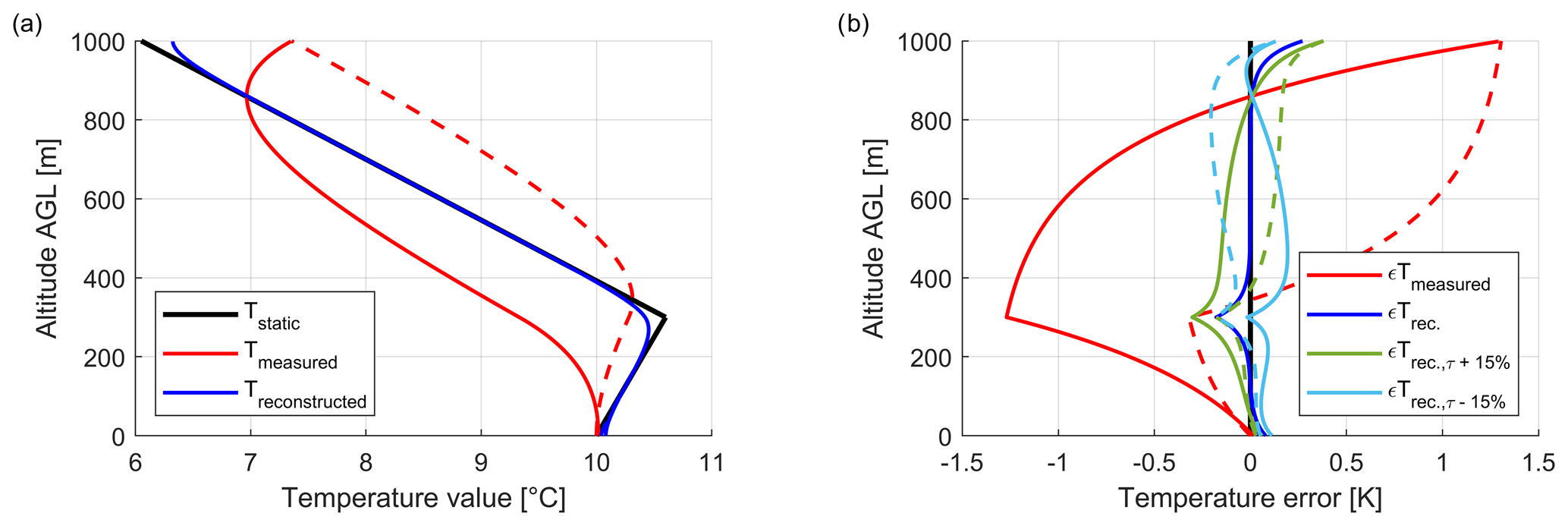
Figure C1(a) A fictional vertical profile of temperature. It is assumed that the drone is moving with a vertical speed of 10 m s−1. In red, the theoretically measured temperature is presented for ascent (dashed line) and descent (solid line), suffering from a time lag with a time constant of 21 s. The blue profile subsequently shows the resulting profile after applying signal reconstruction and subsequently a phase-neutral low-pass filter. (b) The theoretical deviation from the actual profile during ascent (dashed) and descent (solid) for the measured signal and reconstructed signals using the correct time constant τtemp as well as erroneous time constants (τtemp±15 %).
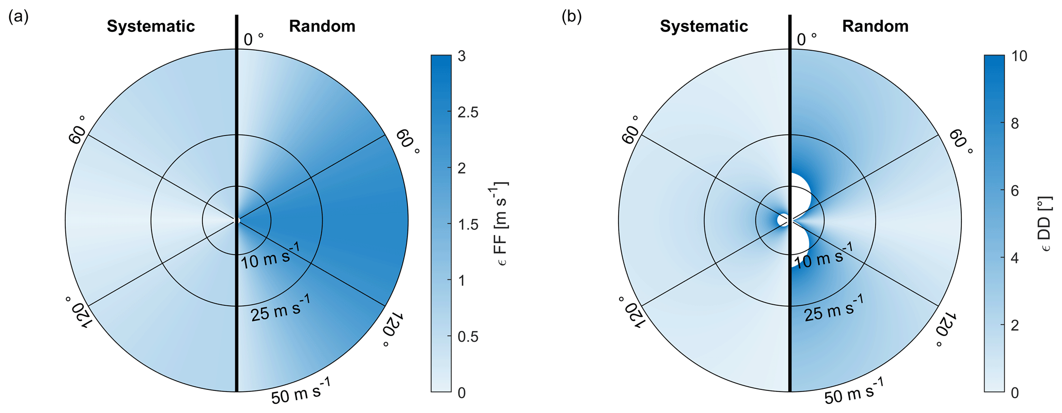
Figure C2Error plots for wind observations, depending on the wind speed and wind incident angle with respect to the course over ground. The colour-coded error is further distinguished between the systematic error caused by a hypothetical vertical air movement of 5 m s−1 and an error in the airspeed calibration factor (uncertainty in the airspeed of 0.2 m s−1) shown on the left halves of the circles and the random error caused by inertial velocity uncertainty (0.1 m s−1 for each component) in addition to an error in the yaw angle Ψ with an uncertainty of 5∘ shown on the right halves. Panel (a) illustrates the subsequent error for wind speed observations, whereas panel (b) reveals systematic as well as random errors in wind direction observations. As the error in the wind direction reaches 180∘ for low-wind conditions, uncertainties above 10∘ are whitened out in the plot.
An illustration of the effect of a time lag on a fictional vertical profile is provided in Fig. C1.
Figure C1a shows the temperature measured with a sensor that incorporates a significant time constant and its deviation during ascent as well as descent. The minimisation of the difference between the profiles during ascent and descent can then be used to determine the time constant of the sensor according to Technique (2). As an additional line in blue, the reconstructed temperature profile using the inverse transfer function of the sensor behaviour is shown. At the reversal points for the temperature gradient and altitude, a small offset is observed, caused by the low-pass filter applied during the signal reconstruction process to eliminate the noise amplified by the reconstruction filter. Figure C1b then shows the correlated errors in temperature observations for the measured temperature, the reconstructed temperature and reconstructed temperatures using an erroneous time constant for the reconstruction filter. The uncertainty in the time constant τtemp is assumed to be ±15 %. Following Eq. (17) in Dirksen et al. (2014), the correlated uncertainty in the temperature caused by an erroneous time constant for signal reconstruction is
with Tmeas,rec(τ) being the measured signal reconstructed with the time constant τ. The additional uncertainty caused by the smoothing filter after the signal reconstruction process ϵTsmooth is roughly estimated as double the magnitude of the error introduced by the time-constant uncertainty ϵTrec for the reconstruction process based on Dirksen et al. (2014), where smoothing after the signal reconstruction using a different filter type than applied here introduces an uncertainty approximately 1 to 2 times larger than the uncertainty according to Eq. (C1).
The maximum error caused by disregarding compressibility (Eq. A4) is determined by calculating the temperature rise for flight parameters and atmospheric values at sea level and at ceiling (10 km) and leads to a theoretical warm bias of ϵTincompress≈0.5 K for the typical flight parameters.
Regarding the error incorporated by an erroneous heat transfer correction factor according to Eq. (A5), assumed to deviate with ±15 %, the measured temperature difference between the fuselage area and the sensor head of up to −40 K results in an error of up to K.
C2 Error estimation of humidity measurements
As the main error sources affecting humidity profiles, daytime solar heating, a sensor lag and a temperature correction are mentioned in Dirksen et al. (2014). The error introduced by solar heating of the HUMICAP sensor is neglected here, since an enclosure protects the sensor from solar radiation. For the calibration uncertainty, data sheet values are adopted. Regarding the time lag, the error introduced by an erroneous time constant for humidity signal reconstruction is prone to potentially high variability and strong gradients for relative humidity in atmospheric profiles. For the estimation of the error, Eq. (C1) is adopted for humidity measurements and time constants, again using a deviation of ±15 % from the assumed correct time constant. Besides the data sheet uncertainty of ϵRH=4 %, the resulting error therefore can only be obtained using observational data.
C3 Error estimation of wind measurements
Neglecting lever-arm-induced velocities leads to an error in wind components of magnitude Ω×r. For typical rotational speeds with σΩ of the LUCA drone and a neglected lever arm of 0.3 m, the uncertainty from neglecting lever arm effects results in an error of up to m s−1 for the vertical and m s−1 for the horizontal lateral (body-fixed) wind component.
The assumption of a zero angle of attack in the first order only influences the vertical wind speed, which will be disregarded in the following, and therefore does not introduce an additional significant error. The assumption of a zero angle of sideslip, however, incorporates an error caused by natural β oscillations of the aircraft. For the LUCA drone, the natural oscillation of 0.7 Hz with an amplitude of around 0.3∘ is irrelevant to the wind and additionally filtered out by averaging the calculated wind in a final step.
The error from neglecting the vertical wind speed, in contrast, potentially leads to significant uncorrelated errors. It is similar to the error introduced by neglecting the vertical velocity of the aircraft, as is assumed in Eq. (A16). Regarding the horizontally projected true airspeed of the aircraft in Eq. (A14), it is evident that the relative error neglecting vertical velocity and the vertical wind speed depends on the ratio of the true airspeed and the vertical velocity/vertical wind speed. Calculating the influence of a neglected vertical speed of 5 m s−1 for an airliner and a fixed-wing drone with hypothetical true airspeeds of 280 m s−1 and 28 m s−1, the deviation from the true airspeed according to Expression (A15) is 0.05 m s−1 for an airliner and 0.45 m s−1 for a fixed-wing drone, directly affecting the wind vector. For the error budget of the LUCA drone, this is neglected for normal measurements, but it should be kept in mind for measurements in strong turbulence.
Another error source leading to a deviation of the retrieved airspeed from the actual airspeed is the pressure calibration coefficient . As the pressure calibration is done by an intrinsic in-flight calibration, comparing flight legs in different directions with respect to the wind, the resulting error in the calibration is below 0.2 m s−1.
The error for inertial position is complex to assess, as multiple sensors are fused in an estimation filter using aircraft states at different integration levels (e.g. acceleration, velocity and position). One can assume that the uncertainty in the velocities estimated by the inertial navigation system on the drone is less than 0.1 m s−1 for each of the three velocity components in vg.
This is similar regarding attitude observations, of which only the yaw angle is needed for wind calculation. Attitude observations of LUCA fuse measurements of the Earth's magnetic field among other measurements and therefore suffer significantly from distortions caused by the electrical system. During climb and generally when the motor of the drone is driven, no wind is calculated as magnetic interferences prevent the attitude estimation from working properly.
The uncertainty in the yaw angle observation on the drone is assumed to be 5∘. From Eq. (A16) using the small-angle approximation sin Ψ≈Ψ, yielding for the easterly wind component, it can be concluded that the wind observation error for an attitude error equals the product of the attitude error and the true airspeed . To reach a comparable uncertainty for the calculated wind, an airliner aircraft (u≈280 m s−1) therefore requires yaw attitude observations that are an order of magnitude lower in uncertainty than the attitude observation uncertainty in a drone with an airspeed of 28 m s−1.
Although uncorrelated errors (e.g. originating from the assumption of β=0 in combination with the aircraft's eigen-oscillations) are likely attenuated during the optional averaging of the calculated wind with a raw data rate of 25 Hz, systematic errors persist. The resulting error for the wind calculation, including systematic errors from neglecting both vertical wind and the airspeed calibration as well as the rather random error sources for inertial velocity and attitude observations, dependent on wind speed and wind direction in relation to aircraft ground course, is presented in Fig. C2, which can be regarded as a graphical elaboration of the error estimation for wind measurements in Vörsmann (1984).
For both wind speed and wind direction, the error in the yaw angle is dominant. For the wind speed, the maximum error of 2.7 m s−1 is seen when the air is moving laterally to the aircraft's course over ground and is independent of the general wind speed, whereas the error in wind direction is maximum with the wind aligned with the aircraft's longitudinal axis (headwind or tailwind) and generally increases towards low wind speed. Neglecting knowledge about wind velocity and direction distribution, the averaged uncertainty fields of the wind observations computed for Fig. C2 are 2.1 m s−1 in magnitude and 7.5∘ in direction.
When it comes to peculiarities of different platform types, one can distinguish three types of platforms: aero-static platforms wandering with the wind speed, Earth-fixed systems such as kites or vertically ascending drones, and fixed-wing aircraft of different sizes and speeds. Based on Eq. (A11), aero-static platforms incorporate with the consequence that only Earth-fixed velocities are needed to calculate wind. Kites or vertically ascending multicopters per definition incorporate , and all transformations and measurements apply to such platforms. Particularly, errors in the vertical velocity assumptions might introduce substantial errors, as the horizontal true airspeed is low in low-wind-speed conditions for kites, tethered balloons or vertically ascending multicopters. Fixed-wing platforms, however, suffer from enhanced angular measurement sensitivity regarding the wind calculation as shown before, which increases with the airspeed of this platform type.
In the following, the temporal variability of temperature, wind speed and relative humidity up to 35 km is illustrated based on ERA5 reanalyses to enable a discussion of the use of additional data observed with drones. To describe the variability of the atmosphere at a specific location and altitude for one parameter, time series of the atmospheric variables can be transformed from the time domain into the frequency domain, e.g. by applying a Fourier transformation. Mapping the results in the frequency domain for every altitude using colours and stacking them over the corresponding altitudes reveal the height-dependent variance of an atmospheric variable on different timescales (herein, the timescale is denoted by cycles per day); e.g. a bright spot for the variable temperature at one cycle per day (period 24 h) close to the surface reveals the diurnal cycle of the temperature in the boundary layer (forced by the sun). Such an analysis of temperature, humidity and wind speed is shown in Fig. D1 for the location of the Lindenberg Meteorological Observatory of the German Weather Service using hourly ERA5 reanalysis data (Hersbach et al., 2023, 2020) for a time span of 1 year. Similar calculations are found in Vinnichenko (1970) and Fiedler and Panofsky (1970), but in contrast to the study of Vinnichenko (1970), which focuses on the kinetic energy spectrum in the free troposphere, and the study of Fiedler and Panofsky (1970), which focuses on spectral gaps, the qualitative fields presented here are used to discuss the benefit of sampling the atmosphere frequently (more than twice a day).
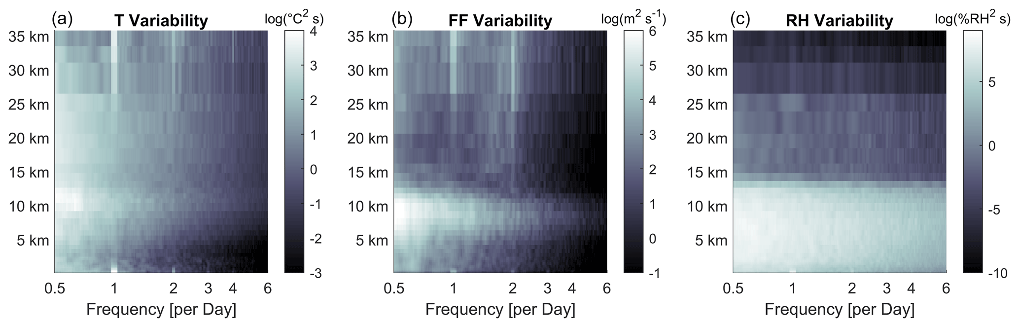
Figure D1Colour-coded mesoscale (periods from 1 to 48 h; Fiedler and Panofsky, 1970) variance densities of time series of atmospheric variables at specific pressure levels (heights). The variances are representative of the atmospheric variability dependent on height and cycles per day (one cycle per day corresponds to a period of 24 h and two cycles per day to 12 h). The data for this analysis originate from the ERA5 reanalysis product. Bright colours indicate high variance density and hence high variability. Panel (a) represents temperature, panel (b) represents wind speed and panel (c) represents humidity.
In Fig. D1a, one can clearly see the diurnal cycle of temperature close to the surface and in the stratosphere through the bright lines at one cycle per day. The bright lines at two cycles per day should not confuse the reader, as the analysis relies on decomposing the time signal in sinusoids with differing frequencies (cycles per day), and higher harmonics (natural products of the fundamental frequency) reveal the non-sinusoidal waveform of the diurnal cycle. Besides in the atmospheric boundary layer, increased variability can be seen at around 10 km altitude for temperature and, after a dip in activity, at around 20 km. Interestingly, temperature variability at six cycles per day is low below 5 km altitude, emphasising the importance of profiling the atmosphere at higher altitudes.
The data are published at PANGAEA and available at https://doi.org/10.1594/PANGAEA.961200 (Bärfuss et al., 2023a) and https://doi.org/10.1594/PANGAEA.961223 (Bärfuss et al., 2023b). Similar datasets obtained with LUCA up to an altitude of 4.5 km are available at https://doi.org/10.1594/PANGAEA.937555 (Bärfuss et al., 2021a) and https://doi.org/10.1594/PANGAEA.937556 (Bärfuss et al., 2021b).
AL and HS developed the project idea and acquired funding. HS and KBB performed the analysis of requirements. KBB developed the LUCA system and the instrumentation. KBB performed the data processing and data analysis. All authors contributed to and reviewed the manuscript.
The contact author has declared that none of the authors has any competing interests.
Publisher’s note: Copernicus Publications remains neutral with regard to jurisdictional claims in published maps and institutional affiliations.
This research has been supported by the Modernity Fund (mFUND) of the German Federal Ministry for Digital and Transport (grant agreement no. 19F2072A).
This open-access publication was funded by Technische Universität Braunschweig.
This paper was edited by Marc von Hobe and reviewed by Ralph Petersen and one anonymous referee.
Archer, C. L. and Caldeira, K.: Historical Trends in the Jet Streams, Geophys. Res. Lett., 35, L08803, https://doi.org/10.1029/2008GL033614, 2008. a
Axford, D. N.: On the Accuracy of Wind Measurements Using an Inertial Platform in an Aircraft, and an Example of a Measurement of the Vertical Mesostructure of the Atmosphere, J. Appl. Meteorol. Climatol., 7, 645–666, https://doi.org/10.1175/1520-0450(1968)007<0645:OTAOWM>2.0.CO;2, 1968. a
Baker, W. E., Atlas, R., Cardinali, C., Clement, A., Emmitt, G. D., Gentry, B. M., Hardesty, R. M., Källén, E., Kavaya, M. J., Langland, R., Ma, Z., Masutani, M., McCarty, W., Pierce, R. B., Pu, Z., Riishojgaard, L. P., Ryan, J., Tucker, S., Weissmann, M., and Yoe, J. G.: Lidar-Measured Wind Profiles: The Missing Link in the Global Observing System, B. Am. Meteorol. Soc., 95, 543–564, https://doi.org/10.1175/BAMS-D-12-00164.1, 2014. a, b
Bange, J., Esposito, M., Lenschow, D. H., Brown, P. R. A., Dreiling, V., Giez, A., Mahrt, L., Malinowski, S. P., Rodi, A. R., Shaw, R. A., Siebert, H., Smit, H., and Zöger, M.: Measurement of Aircraft State and Thermodynamic and Dynamic Variables, in: Airborne Measurements for Environmental Research, Chap. 2, 7–75, John Wiley & Sons, Ltd, https://doi.org/10.1002/9783527653218.ch2, 2013. a, b, c
Bärfuss, K., Pätzold, F., Altstädter, B., Kathe, E., Nowak, S., Bretschneider, L., Bestmann, U., and Lampert, A.: New Setup of the UAS ALADINA for Measuring Boundary Layer Properties, Atmospheric Particles and Solar Radiation, Atmosphere, 9, 28, https://doi.org/10.3390/atmos9010028, 2018. a, b, c, d, e, f, g
Bärfuss, K., Schmithüsen, H., Dirksen, R., Bretschneider, L., Pätzold, F., Bollmann, S., Wickboldt, H., von Unwerth, M., Asmussen, M., Schwarting, T., and Lampert, A.: Atmospheric Profile Measurements Conducted by the Unmanned Aerial System LUCA (Panker, Germany, 2020-07-03 and 2021-05-28), PANGAEA [data set], https://doi.org/10.1594/PANGAEA.937555, 2021a. a, b
Bärfuss, K., Schmithüsen, H., Dirksen, R., Bretschneider, L., Pätzold, F., Bollmann, S., Wickboldt, H., von Unwerth, M., Asmussen, M., Schwarting, T., and Lampert, A.: Radiosonde Measurements Co-Located with Ascends of the Unmanned Aerial System LUCA (Panker, Germany 2020-07-03 and 2021-05-28), PANGAEA [data set], https://doi.org/10.1594/PANGAEA.937556, 2021b. a
Bärfuss, K. B., Schmithüsen, H., and Lampert, A.: Drone-based meteorological observations up to the tropopause, Atmos. Meas. Tech. Discuss. [preprint], https://doi.org/10.5194/amt-2022-236, in review, 2022. a, b, c, d, e
Bärfuss, K., Wickboldt, H., Schlerf, A., Bollmann, S., Rausch, T., and Lampert, A.: Atmospheric profile measurements conducted by the unmanned aerial system LUCA (Panker, Germany 2021-10-25 to 2021-10-29), PANGAEA [data set], https://doi.org/10.1594/PANGAEA.961200, 2023a. a
Bärfuss, K., Wickboldt, H., Schlerf, A., Bollmann, S., Rausch, T., and Lampert, A.: Radiosonde measurements co-located with ascends of the unmanned aerial system LUCA (Panker, Germany 2021-10-25 and 2021-10-29), PANGAEA [data set], https://doi.org/10.1594/PANGAEA.961223, 2023b. a
Bauer, P., Thorpe, A., and Brunet, G.: The Quiet Revolution of Numerical Weather Prediction, Nature, 525, 47–55, https://doi.org/10.1038/nature14956, 2015. a
Bonavita, M., Hólm, E., Isaksen, L., and Fisher, M.: The Evolution of the ECMWF Hybrid Data Assimilation System, Q. J. Roy. Meteorol. Soc., 142, 287–303, https://doi.org/10.1002/qj.2652, 2016. a
Bormann, N., Lawrence, H., Farnan, J., and Farnan, J.: Global Observing System Experiments in the ECMWF Assimilation System, ECMWF, https://doi.org/10.21957/sr184iyz, 2019. a, b
Bouttier, F. and Kelly, G.: Observing-System Experiments in the ECMWF 4D-Var Data Assimilation System, Q. J. Roy. Meteorol. Soc., 127, 1469–1488, https://doi.org/10.1002/qj.49712757419, 2001. a, b
Boylan, P., Wang, J., Cohn, S. A., Fetzer, E., Maddy, E. S., and Wong, S.: Validation of AIRS Version 6 Temperature Profiles and Surface-Based Inversions over Antarctica Using Concordiasi Dropsonde Data, J. Geophys. Res.-Atmos., 120, 992–1007, https://doi.org/10.1002/2014JD022551, 2015. a
Cardinali, C.: Monitoring the Observation Impact on the Short-Range Forecast, Q. J. Roy. Meteorol. Soc., 135, 239–250, https://doi.org/10.1002/qj.366, 2009. a
Cardinali, C.: Observation Impact on the Short Range Forecast, https://www.ecmwf.int/node/16937 (last access: 1 August 2023), 2013. a
Carminati, F., Migliorini, S., Ingleby, B., Bell, W., Lawrence, H., Newman, S., Hocking, J., and Smith, A.: Using reference radiosondes to characterise NWP model uncertainty for improved satellite calibration and validation, Atmos. Meas. Tech., 12, 83–106, https://doi.org/10.5194/amt-12-83-2019, 2019. a, b
Chander, G., Hewison, T. J., Fox, N., Wu, X., Xiong, X., and Blackwell, W. J.: Overview of Intercalibration of Satellite Instruments, IEEE Trans. Geosci. Remote Sens., 51, 1056–1080, https://doi.org/10.1109/TGRS.2012.2228654, 2013. a
Chilson, P. B., Bell, T. M., Brewster, K. A., Britto Hupsel de Azevedo, G., Carr, F. H., Carson, K., Doyle, W., Fiebrich, C. A., Greene, B. R., Grimsley, J. L., Kanneganti, S. T., Martin, J., Moore, A., Palmer, R. D., Pillar-Little, E. A., Salazar-Cerreno, J. L., Segales, A. R., Weber, M. E., Yeary, M., and Droegemeier, K. K.: Moving towards a Network of Autonomous UAS Atmospheric Profiling Stations for Observations in the Earth's Lower Atmosphere: The 3D Mesonet Concept, Sensors, 19, 2720, https://doi.org/10.3390/s19122720, 2019. a
Choi, B. I., Lee, S.-W., Woo, S.-B., Kim, J. C., Kim, Y.-G., and Yang, S. G.: Evaluation of radiosonde humidity sensors at low temperature using ultralow-temperature humidity chamber, Adv. Sci. Res., 15, 207–212, https://doi.org/10.5194/asr-15-207-2018, 2018. a, b
Cione, J. J., Bryan, G. H., Dobosy, R., Zhang, J. A., de Boer, G., Aksoy, A., Wadler, J. B., Kalina, E. A., Dahl, B. A., Ryan, K., Neuhaus, J., Dumas, E., Marks, F. D., Farber, A. M., Hock, T., and Chen, X.: Eye of the Storm: Observing Hurricanes with a Small Unmanned Aircraft System, B. Am. Meteorol. Soc., 101, E186–E205, https://doi.org/10.1175/BAMS-D-19-0169.1, 2020. a
Cohn, S. A., Hock, T., Cocquerez, P., Wang, J., Rabier, F., Parsons, D., Harr, P., Wu, C.-C., Drobinski, P., Karbou, F., Vénel, S., Vargas, A., Fourrié, N., Saint-Ramond, N., Guidard, V., Doerenbecher, A., Hsu, H.-H., Lin, P.-H., Chou, M.-D., Redelsperger, J.-L., Martin, C., Fox, J., Potts, N., Young, K., and Cole, H.: Driftsondes: Providing In Situ Long-Duration Dropsonde Observations over Remote Regions, B. Am. Meteorol. Soc., 94, 1661–1674, https://doi.org/10.1175/BAMS-D-12-00075.1, 2013. a
Cooper, W. A., Spuler, S. M., Spowart, M., Lenschow, D. H., and Friesen, R. B.: Calibrating airborne measurements of airspeed, pressure and temperature using a Doppler laser air-motion sensor, Atmos. Meas. Tech., 7, 3215–3231, https://doi.org/10.5194/amt-7-3215-2014, 2014. a
Dabberdt, W. F., Schlatter, T. W., Carr, F. H., Friday, E. W. J., Jorgensen, D., Koch, S., Pirone, M., Ralph, F. M., Sun, J., Welsh, P., Wilson, J. W., and Zou, X.: Multifunctional Mesoscale Observing Networks, B. Am. Meteorol. Soc., 86, 961–982, https://doi.org/10.1175/BAMS-86-7-961, 2005. a, b
de Boer, G., Diehl, C., Jacob, J., Houston, A., Smith, S. W., Chilson, P., Schmale, D. G., Intrieri, J., Pinto, J., Elston, J., Brus, D., Kemppinen, O., Clark, A., Lawrence, D., Bailey, S. C. C., Sama, M. P., Frazier, A., Crick, C., Natalie, V., Pillar-Little, E., Klein, P., Waugh, S., Lundquist, J. K., Barbieri, L., Kral, S. T., Jensen, A. A., Dixon, C., Borenstein, S., Hesselius, D., Human, K., Hall, P., Argrow, B., Thornberry, T., Wright, R., and Kelly, J. T.: Development of Community, Capabilities, and Understanding through Unmanned Aircraft-Based Atmospheric Research: The LAPSE-RATE Campaign, B. Am. Meteorol. Soc., 101, E684–E699, https://doi.org/10.1175/BAMS-D-19-0050.1, 2020. a
de Haan, S., de Jong, P. M. A., and van der Meulen, J.: Characterizing and correcting the warm bias observed in Aircraft Meteorological Data Relay (AMDAR) temperature observations, Atmos. Meas. Tech., 15, 811–818, https://doi.org/10.5194/amt-15-811-2022, 2022. a
Dirksen, R. J., Sommer, M., Immler, F. J., Hurst, D. F., Kivi, R., and Vömel, H.: Reference quality upper-air measurements: GRUAN data processing for the Vaisala RS92 radiosonde, Atmos. Meas. Tech., 7, 4463–4490, https://doi.org/10.5194/amt-7-4463-2014, 2014. a, b, c, d, e, f, g
Drüe, C., Frey, W., Hoff, A., and Hauf, Th.: Aircraft Type-Specific Errors in AMDAR Weather Reports from Commercial Aircraft, Q. J. Roy. Meteorol. Soc., 134, 229–239, https://doi.org/10.1002/qj.205, 2008. a, b
Dupont, J.-C., Haeffelin, M., Badosa, J., Clain, G., Raux, C., and Vignelles, D.: Characterization and Corrections of Relative Humidity Measurement from Meteomodem M10 Radiosondes at Midlatitude Stations, J. Atmos. Ocean. Technol., 37, 857–871, https://doi.org/10.1175/JTECH-D-18-0205.1, 2020. a
EASA: Easy Access Rules for Unmanned Aircraft Systems (Regulation (EU) 2019/947 and Regulation (EU) 2019/945), https://www.easa.europa.eu/document-library/easy-access-rules/easy-access-rules-unmanned-aircraft-systems-regulation-eu (last access: 1 August 2023), 2022. a, b
Elston, J., Argrow, B., Stachura, M., Weibel, D., Lawrence, D., and Pope, D.: Overview of Small Fixed-Wing Unmanned Aircraft for Meteorological Sampling, J. Atmos. Ocean. Technol., 32, 97–115, https://doi.org/10.1175/JTECH-D-13-00236.1, 2015. a
Elston, J. S., Roadman, J., Stachura, M., Argrow, B., Houston, A., and Frew, E.: The Tempest Unmanned Aircraft System for in Situ Observations of Tornadic Supercells: Design and VORTEX2 Flight Results, J. Field Robot., 28, 461–483, https://doi.org/10.1002/rob.20394, 2011. a
Evtushevsky, O. M., Grytsai, A. V., Klekociuk, A. R., and Milinevsky, G. P.: Total Ozone and Tropopause Zonal Asymmetry during the Antarctic Spring, J. Geophys. Res.-Atmos., 113, D00B06, https://doi.org/10.1029/2008JD009881, 2008. a
Eyre, J.: An Introduction to GPS Radio Occultation and Its Use in Numerical Weather Prediction., in: ECMWF GRAS SAF Workshop on Applications of GPS Radio Occultation Measurements, 16–18 June 2008, 1–10, ECMWF, Shinfield Park, Reading, 2008. a
Faccani, C., Rabier, F., Fourrié, N., Agusti-Panareda, A., Karbou, F., Moll, P., Lafore, J.-P., Nuret, M., Hdidou, F., and Bock, O.: The Impacts of AMMA Radiosonde Data on the French Global Assimilation and Forecast System, Weather Forecast., 24, 1268–1286, https://doi.org/10.1175/2009WAF2222237.1, 2009. a, b
Fiedler, F. and Panofsky, H. A.: Atmospheric Scales and Spectral Gaps, B. Am. Meteorol. Soc., 51, 1114–1120, https://doi.org/10.1175/1520-0477(1970)051<1114:ASASG>2.0.CO;2, 1970. a, b, c
Flagg, D. D., Doyle, J. D., Holt, T. R., Tyndall, D. P., Amerault, C. M., Geiszler, D., Haack, T., Moskaitis, J. R., Nachamkin, J., and Eleuterio, D. P.: On the Impact of Unmanned Aerial System Observations on Numerical Weather Prediction in the Coastal Zone, Mon. Weather Rev., 146, 599–622, https://doi.org/10.1175/MWR-D-17-0028.1, 2018. a
Fleming, R. J.: The Use of Commercial Aircraft as Platforms for Environmental Measurements, B. Am. Meteorol. Soc., 77, 2229–2242, https://doi.org/10.1175/1520-0477(1996)077<2229:TUOCAA>2.0.CO;2, 1996. a
Fujiwara, M., Shiotani, M., Hasebe, F., Vömel, H., Oltmans, S. J., Ruppert, P. W., Horinouchi, T., and Tsuda, T.: Performance of the Meteolabor “Snow White” Chilled-Mirror Hygrometer in the Tropical Troposphere: Comparisons with the Vaisala RS80 A/H-Humicap Sensors, J. Atmos. Ocean. Technol., 20, 1534–1542, https://doi.org/10.1175/1520-0426(2003)020<1534:POTMSW>2.0.CO;2, 2003. a
Geerts, B., Raymond, D. J., Grubišić, V., Davis, C. A., Barth, M. C., Detwiler, A., Klein, P. M., Lee, W.-C., Markowski, P. M., Mullendore, G. L., and Moore, J. A.: Recommendations for In Situ and Remote Sensing Capabilities in Atmospheric Convection and Turbulence, B. Am. Meteorol. Soc., 99, 2463–2470, https://doi.org/10.1175/BAMS-D-17-0310.1, 2018. a, b
Gelaro, R. and Zhu, Y.: Examination of Observation Impacts Derived from Observing System Experiments (OSEs) and Adjoint Models, Tellus A, 61, 179–193, https://doi.org/10.1111/j.1600-0870.2008.00388.x, 2009. a
Gettelman, A., Hoor, P., Pan, L. L., Randel, W. J., Hegglin, M. I., and Birner, T.: The Extratropical Upper Troposphere and Lower Stratosphere, Rev. Geophys., 49, RG3003, https://doi.org/10.1029/2011RG000355, 2011. a
Goldberg, M., Ohring, G., Butler, J., Cao, C., Datla, R., Doelling, D., Gärtner, V., Hewison, T., Iacovazzi, B., Kim, D., Kurino, T., Lafeuille, J., Minnis, P., Renaut, D., Schmetz, J., Tobin, D., Wang, L., Weng, F., Wu, X., Yu, F., Zhang, P., and Zhu, T.: The Global Space-Based Inter-Calibration System, B. Am. Meteorol. Soc., 92, 467–475, https://doi.org/10.1175/2010BAMS2967.1, 2011. a
Hacker, J., Draper, C., and Madaus, L.: Challenges and Opportunities for Data Assimilation in Mountainous Environments, Atmosphere, 9, 127, https://doi.org/10.3390/atmos9040127, 2018. a
Haering, E. Jr.: Airdata Calibration of a High-Performance Aircraft for Measuring Atmospheric Wind Profiles, in: 28th Aerospace Sciences Meeting, Aerospace Sciences Meetings, American Institute of Aeronautics and Astronautics, https://doi.org/10.2514/6.1990-230, 1990. a
Hann, R.: Atmospheric Ice Accretions, Aerodynamic Icing Penalties, and Ice Protection Systems on Unmanned Aerial Vehicles, NTNU, https://ntnuopen.ntnu.no/ntnu-xmlui/handle/11250/2657638 (last access: 1 August 2023), 2020. a
Hann, R., Enache, A., Nielsen, M. C., Stovner, B. N., van Beeck, J., Johansen, T. A., and Borup, K. T.: Experimental Heat Loads for Electrothermal Anti-Icing and De-Icing on UAVs, Aerospace, 8, 83, https://doi.org/10.3390/aerospace8030083, 2021. a
Hartmann, J., Gehrmann, M., Kohnert, K., Metzger, S., and Sachs, T.: New calibration procedures for airborne turbulence measurements and accuracy of the methane fluxes during the AirMeth campaigns, Atmos. Meas. Tech., 11, 4567–4581, https://doi.org/10.5194/amt-11-4567-2018, 2018. a
Hersbach, H., Bell, B., Berrisford, P., Biavati, G., Horányi, A., Muñoz Sabater, J., Nicolas, J., Peubey, C., Radu, R., Rozum, I., Schepers, D., Simmons, A., Soci, C., Dee, D., and Thépaut, J.-N.: ERA5 hourly data on single levels from 1940 to present, Copernicus Climate Change Service (C3S) Climate Data Store (CDS) [data set], https://doi.org/10.24381/cds.adbb2d47, 2023. a, b
Hersbach, H., Bell, B., Berrisford, P., Hirahara, S., Horányi, A., Muñoz-Sabater, J., Nicolas, J., Peubey, C., Radu, R., Schepers, D., Simmons, A., Soci, C., Abdalla, S., Abellan, X., Balsamo, G., Bechtold, P., Biavati, G., Bidlot, J., Bonavita, M., Chiara, G., Dahlgren, P., Dee, D., Diamantakis, M., Dragani, R., Flemming, J., Forbes, R., Fuentes, M., Geer, A., Haimberger, L., Healy, S., Hogan, R. J., Hólm, E., Janisková, M., Keeley, S., Laloyaux, P., Lopez, P., Lupu, C., Radnoti, G., Rosnay, P., Rozum, I., Vamborg, F., Villaume, S., and Thépaut, J.-N.: The ERA5 Global Reanalysis, Q. J. Roy. Meteorol. Soc., 146, 1999–2049, https://doi.org/10.1002/qj.3803, 2020. a, b, c
Hock, T. F. and Franklin, J. L.: The NCAR GPS Dropwindsonde, B. Am. Meteorol. Soc., 80, 407–420, 1999. a
Holton, J. R., Haynes, P. H., McIntyre, M. E., Douglass, A. R., Rood, R. B., and Pfister, L.: Stratosphere-Troposphere Exchange, Rev. Geophys., 33, 403–439, https://doi.org/10.1029/95RG02097, 1995. a
Houston, A. L., PytlikZillig, L. M., and Walther, J. C.: National Weather Service Data Needs for Short-Term Forecasts and the Role of Unmanned Aircraft in Filling the Gap: Results from a Nationwide Survey, B. Am. Meteorol. Soc., 102, E2106–E2120, https://doi.org/10.1175/BAMS-D-20-0183.1, 2021. a, b
Huang, X., Tepylo, N., Pommier-Budinger, V., Budinger, M., Bonaccurso, E., Villedieu, P., and Bennani, L.: A Survey of Icephobic Coatings and Their Potential Use in a Hybrid Coating/Active Ice Protection System for Aerospace Applications, Prog. Aerospace Sci., 105, 74–97, https://doi.org/10.1016/j.paerosci.2019.01.002, 2019. a
Ingleby, B. and Edwards, D.: Changes to Radiosonde Reports and Their Processing for Numerical Weather Prediction, Atmos. Sc. Lett., 16, 44–49, https://doi.org/10.1002/asl2.518, 2015. a, b, c
Ingleby, B., Pauley, P., Kats, A., Ator, J., Keyser, D., Doerenbecher, A., Fucile, E., Hasegawa, J., Toyoda, E., Kleinert, T., Qu, W., James, J. S., Tennant, W., and Weedon, R.: Progress toward High-Resolution, Real-Time Radiosonde Reports, B. Am. Meteorol. Soc., 97, 2149–2161, https://doi.org/10.1175/BAMS-D-15-00169.1, 2016a. a
Ingleby, B., Rodwell, M., and Isaksen, L.: Global Radiosonde Network under Pressure, Tech. Rep. 149, ECMWF, https://doi.org/10.21957/cblxtg, 2016b. a
Ingleby, B., Isaksen, L., Kral, T., and Kral, T.: Evaluation and Impact of Aircraft Humidity Data in ECMWF's NWP System, https://doi.org/10.21957/4e825dtiy, 2020. a, b
Ingleby, B., Candy, B., Eyre, J., Haiden, T., Hill, C., Isaksen, L., Kleist, D., Smith, F., Steinle, P., Taylor, S., Tennant, W., and Tingwell, C.: The Impact of COVID-19 on Weather Forecasts: A Balanced View, Geophys. Res. Lett., 48, e2020GL090699, https://doi.org/10.1029/2020GL090699, 2021. a
Ingleby, B., Motl, M., Marlton, G., Edwards, D., Sommer, M., von Rohden, C., Vömel, H., and Jauhiainen, H.: On the quality of RS41 radiosonde descent data, Atmos. Meas. Tech., 15, 165–183, https://doi.org/10.5194/amt-15-165-2022, 2022. a, b, c, d
Inoue, J. and Sato, K.: Toward Sustainable Meteorological Profiling in Polar Regions: Case Studies Using an Inexpensive UAS on Measuring Lower Boundary Layers with Quality of Radiosondes, Environ. Res., 205, 112468, https://doi.org/10.1016/j.envres.2021.112468, 2022. a, b, c
Jacob, J. D., Chilson, P. B., Houston, A. L., and Smith, S. W.: Considerations for Atmospheric Measurements with Small Unmanned Aircraft Systems, Atmosphere, 9, 252, https://doi.org/10.3390/atmos9070252, 2018. a
Jeck, R. K.: Icing Design Envelopes (14 CFR Parts 25 and 29, Appendix C) Converted to a Distance-Based Format, Federal Aviation Administration Report DOT/FAA/AR-00/30, US Department of Transportation, Washington, DC, USA, 2002. a
Jensen, A. A., Pinto, J. O., Bailey, S. C., Sobash, R. A., de Boer, G., Houston, A. L., Chilson, P. B., Bell, T., Romine, G., Smith, S. W., Lawrence, D. A., Dixon, C., Lundquist, J. K., Jacob, J. D., Elston, J., Waugh, S., and Steiner, M.: Assimilation of a Coordinated Fleet of Uncrewed Aircraft System Observations in Complex Terrain: EnKF System Design and Preliminary Assessment, Mon. Weather Rev., 149, 1459–1480, https://doi.org/10.1175/mwr-d-20-0359.1, 2021. a
Jensen, A. A., Pinto, J. O., Bailey, S. C. C., Sobash, R. A., Romine, G., de Boer, G., Houston, A. L., Smith, S. W., Lawrence, D. A., Dixon, C., Lundquist, J. K., Jacob, J. D., Elston, J., Waugh, S., Brus, D., and Steiner, M.: Assimilation of a Coordinated Fleet of Uncrewed Aircraft System Observations in Complex Terrain: Observing System Experiments, Mon. Weather Rev., 150, 2737–2763, https://doi.org/10.1175/MWR-D-22-0090.1, 2022. a
Jonassen, M. O., Ólafsson, H., Ágústsson, H., Rögnvaldsson, Ó., and Reuder, J.: Improving High-Resolution Numerical Weather Simulations by Assimilating Data from an Unmanned Aerial System, Mon. Weather Rev., 140, 3734–3756, https://doi.org/10.1175/MWR-D-11-00344.1, 2012. a
Joyce, K. E., Anderson, K., and Bartolo, R. E.: Of Course We Fly Unmanned – We're Women!, Drones, 5, 21, https://doi.org/10.3390/drones5010021, 2021. a
Kalinka, F., Roloff, K., Tendel, J., and Hauf, T.: The In-flight Icing Warning System ADWICE for European Airspace – Current Structure, Recent Improvements and Verification Results, Meteorologische Z., 26, 441–455, https://doi.org/10.1127/metz/2017/0756, 2017. a
Kalman, R. E.: A New Approach to Linear Filtering and Prediction Problems, J. Basic Eng., 82, 35–45, https://doi.org/10.1115/1.3662552, 1960. a
Karbou, F., Aires, F., Prigent, C., and Eymard, L.: Potential of Advanced Microwave Sounding Unit-A (AMSU-A) and AMSU-B Measurements for Atmospheric Temperature and Humidity Profiling over Land, J. Geophys. Res.-Atmos., 110, D07109, https://doi.org/10.1029/2004JD005318, 2005. a, b
Kim, S.-M. and Kim, H. M.: Forecast Sensitivity Observation Impact in the 4DVAR and Hybrid-4DVAR Data Assimilation Systems, J. Atmos. Ocean. Technol., 36, 1563–1575, https://doi.org/10.1175/JTECH-D-18-0240.1, 2019. a
Koch, S. E., Fengler, M., Chilson, P. B., Elmore, K. L., Argrow, B., Andra, D. L., and Lindley, T.: On the Use of Unmanned Aircraft for Sampling Mesoscale Phenomena in the Preconvective Boundary Layer, J. Atmos. Ocean. Technol., 35, 2265–2288, https://doi.org/10.1175/JTECH-D-18-0101.1, 2018. a
König-Langlo, G., King, J. C., and Pettré, P.: Climatology of the Three Coastal Antarctic Stations Dumont d'Urville, Neumayer, and Halley, J. Geophys. Res.-Atmos., 103, 10935–10946, https://doi.org/10.1029/97JD00527, 1998. a
Konrad, T., Hill, M., Rowland, J., and Meyer, J. H.: A Small, Radio-Controlled Aircraft as a Platform for Meteorological Sensors, Johns Hopkins APL Tech. Dig., 10, 11–21, 1970. a
Kotthaus, S., Bravo-Aranda, J. A., Collaud Coen, M., Guerrero-Rascado, J. L., Costa, M. J., Cimini, D., O'Connor, E. J., Hervo, M., Alados-Arboledas, L., Jiménez-Portaz, M., Mona, L., Ruffieux, D., Illingworth, A., and Haeffelin, M.: Atmospheric boundary layer height from ground-based remote sensing: a review of capabilities and limitations, Atmos. Meas. Tech., 16, 433–479, https://doi.org/10.5194/amt-16-433-2023, 2023. a
Kräuchi, A. and Philipona, R.: Return glider radiosonde for in situ upper-air research measurements, Atmos. Meas. Tech., 9, 2535–2544, https://doi.org/10.5194/amt-9-2535-2016, 2016. a
Kren, A. C., Cucurull, L., and Wang, H.: Impact of UAS Global Hawk Dropsonde Data on Tropical and Extratropical Cyclone Forecasts in 2016, Weather Forecast., 33, 1121–1141, https://doi.org/10.1175/WAF-D-18-0029.1, 2018. a, b
Lafon, T., Fowler, J., Jiménez, J. F., and Cordoba, G. J. T.: A Viable Alternative for Conducting Cost-Effective Daily Atmospheric Soundings in Developing Countries, B. Am. Meteorol. Soc., 95, 837–842, https://doi.org/10.1175/BAMS-D-13-00125.1, 2014. a
Lampert, A., Altstädter, B., Bärfuss, K., Bretschneider, L., Sandgaard, J., Michaelis, J., Lobitz, L., Asmussen, M., Damm, E., Käthner, R., Krüger, T., Lüpkes, C., Nowak, S., Peuker, A., Rausch, T., Reiser, F., Scholtz, A., Sotomayor Zakharov, D., Gaus, D., Bansmer, S., Wehner, B., and Pätzold, F.: Unmanned Aerial Systems for Investigating the Polar Atmospheric Boundary Layer – Technical Challenges and Examples of Applications, Atmosphere, 11, 416, https://doi.org/10.3390/atmos11040416, 2020. a, b, c, d
Langland, R. H. and Baker, N. L.: Estimation of Observation Impact Using the NRL Atmospheric Variational Data Assimilation Adjoint System, Tellus A. 56, 189–201, https://doi.org/10.3402/tellusa.v56i3.14413, 2004. a
Laursen, K. K., Jorgensen, D. P., Brasseur, G. P., Ustin, S. L., and Huning, J. R.: HIAPER: THE NEXT GENERATION NSF/NCAR RESEARCH AIRCRAFT, B. Am. Meteorol. Soc., 87, 896–909, 2006. a
Lenschow, H.: The Measurement of Air Velocity and Temperature Using the NCAR Buffalo Aircraft Measuring System, Technical Report NCAR/TN-74+EDD, University Corporation for Atmospheric Research, https://opensky.ucar.edu/islandora/object/technotes:62/ (last access: 1 August 2023), 1972. a, b
Leuenberger, D., Haefele, A., Omanovic, N., Fengler, M., Martucci, G., Calpini, B., Fuhrer, O., and Rossa, A.: Improving High-Impact Numerical Weather Prediction with Lidar and Drone Observations, B. Am. Meteorol. Soc., 101, E1036–E1051, https://doi.org/10.1175/BAMS-D-19-0119.1, 2020. a, b, c, d, e, f
Lindskog, M., Salonen, K., Järvinen, H., and Michelson, D. B.: Doppler Radar Wind Data Assimilation with HIRLAM 3DVAR, Mon. Weather Rev., 132, 1081–1092, https://doi.org/10.1175/1520-0493(2004)132<1081:DRWDAW>2.0.CO;2, 2004. a
Lorenc, A. C. and Marriott, R. T.: Forecast Sensitivity to Observations in the Met Office Global Numerical Weather Prediction System, Q. J. Roy. Meteorol. Soc., 140, 209–224, https://doi.org/10.1002/qj.2122, 2014. a
Majewski, J.: The Dynamic Behaviour of Capacitive Humidity Sensors, Devices and Methods of Measurements, 11, 53–59, https://doi.org/10.21122/2220-9506-2020-11-1-53-59, 2020. a, b
Mallaun, C., Giez, A., and Baumann, R.: Calibration of 3-D wind measurements on a single-engine research aircraft, Atmos. Meas. Tech., 8, 3177–3196, https://doi.org/10.5194/amt-8-3177-2015, 2015. a
Miloshevich, L. M., Paukkunen, A., Vömel, H., and Oltmans, S. J.: Development and Validation of a Time-Lag Correction for Vaisala Radiosonde Humidity Measurements, J. Atmos. Ocean. Technol., 21, 1305–1327, https://doi.org/10.1175/1520-0426(2004)021<1305:DAVOAT>2.0.CO;2, 2004. a, b, c
Moninger, W. R., Mamrosh, R. D., and Pauley, P. M.: Automated Meteorological Reports from Commercial Aircraft, B. Am. Meteorol. Soc., 84, 203–216, https://doi.org/10.1175/BAMS-84-2-203, 2003. a
Moninger, W. R., Benjamin, S. G., Jamison, B. D., Schlatter, T. W., Smith, T. L., and Szoke, E. J.: Evaluation of Regional Aircraft Observations Using TAMDAR, Weather Forecast., 25, 627–645, https://doi.org/10.1175/2009WAF2222321.1, 2010. a
Nash, J., Oakley, T., Vömel, H., and Wei, L.: IOM Report, 107. WMO Intercomparison of High Quality Radiosonde Systems, WMO/TD, World Meteorological Organization, Geneva, 249 pp., https://library.wmo.int/doc_num.php?explnum_id=9467 (last access: 1 August 2023), 2011. a, b
Ota, Y., Derber, J. C., Kalnay, E., and Miyoshi, T.: Ensemble-Based Observation Impact Estimates Using the NCEP GFS, Tellus A, 65, 20038, https://doi.org/10.3402/tellusa.v65i0.20038, 2013. a, b, c
Palmer, R., Whelan, D., Bodine, D., Kirstetter, P., Kumjian, M., Metcalf, J., Yeary, M., Yu, T.-Y., Rao, R., Cho, J., Draper, D., Durden, S., English, S., Kollias, P., Kosiba, K., Wada, M., Wurman, J., Blackwell, W., Bluestein, H., Collis, S., Gerth, J., Tuttle, A., Wang, X., and Zrnić, D.: The Need for Spectrum and the Impact on Weather Observations, B. Am. Meteorol. Soc., 102, E1402–E1407, https://doi.org/10.1175/BAMS-D-21-0009.1, 2021. a, b
Pätzold, F.: Windmessung mittels Segelflugzeug, Forschungsbericht 2018-04, Niedersächsisches Forschungszentrum für Luftfahrt, Braunschweig, Germany, https://doi.org/10.24355/dbbs.084-201805221102-1, 2018. a
Pena-Ortiz, C., Gallego, D., Ribera, P., Ordonez, P., and Alvarez-Castro, M. D. C.: Observed Trends in the Global Jet Stream Characteristics during the Second Half of the 20th Century, J. Geophys. Res.-Atmos., 118, 2702–2713, https://doi.org/10.1002/jgrd.50305, 2013. a
Petersen, R. A.: On the Impact and Benefits of AMDAR Observations in Operational Forecasting – Part I: A Review of the Impact of Automated Aircraft Wind and Temperature Reports, B. Am. Meteorol. Soc., 97, 585–602, https://doi.org/10.1175/BAMS-D-14-00055.1, 2016. a, b, c
Petersen, R. A., Cronce, L., Mamrosh, R., and Baker, R.: A Report to the World Meteorological Organization on the Impact and Benefits of AMDAR Temperature, Wind and Moisture Observations in Operational Weather Forecasting, Tech. rep., University of Wisconsin-Madison, Cooperative Institute for Meteorological Satellite Studies, Space Science and Engineering center, https://search.library.wisc.edu/catalog/9911154629902121 (last access: 1 August 2023), 2015. a
Petersen, R. A., Cronce, L., Mamrosh, R., Baker, R., and Pauley, P.: On the Impact and Future Benefits of AMDAR Observations in Operational Forecasting: Part II: Water Vapor Observations, B. Am. Meteorol. Soc., 97, 2117–2133, https://doi.org/10.1175/BAMS-D-14-00211.1, 2016. a, b, c
Pinto, J. O., O'Sullivan, D., Taylor, S., Elston, J., Baker, C. B., Hotz, D., Marshall, C., Jacob, J., Barfuss, K., Piguet, B., Roberts, G., Omanovic, N., Fengler, M., Jensen, A. A., Steiner, M., and Houston, A. L.: The Status and Future of Small Uncrewed Aircraft Systems (UAS) in Operational Meteorology, B. Am. Meteorol. Soc., 102, E2121–E2136, https://doi.org/10.1175/BAMS-D-20-0138.1, 2021. a, b, c, d, e
Rabier, F., Bouchard, A., Brun, E., Doerenbecher, A., Guedj, S., Guidard, V., Karbou, F., Peuch, V.-H., Amraoui, L. E., Puech, D., Genthon, C., Picard, G., Town, M., Hertzog, A., Vial, F., Cocquerez, P., Cohn, S. A., Hock, T., Fox, J., Cole, H., Parsons, D., Powers, J., Romberg, K., VanAndel, J., Deshler, T., Mercer, J., Haase, J. S., Avallone, L., Kalnajs, L., Mechoso, C. R., Tangborn, A., Pellegrini, A., Frenot, Y., Thépaut, J.-N., McNally, A., Balsamo, G., and Steinle, P.: The Concordiasi Project in Antarctica, B. Am. Meteorol. Soc., 91, 69–86, https://doi.org/10.1175/2009BAMS2764.1, 2010. a
Ralph, F. M., Cannon, F., Tallapragada, V., Davis, C. A., Doyle, J. D., Pappenberger, F., Subramanian, A., Wilson, A. M., Lavers, D. A., Reynolds, C. A., Haase, J. S., Centurioni, L., Ingleby, B., Rutz, J. J., Cordeira, J. M., Zheng, M., Hecht, C., Kawzenuk, B., and Monache, L. D.: West Coast Forecast Challenges and Development of Atmospheric River Reconnaissance, B. Am. Meteorol. Soc., 101, E1357–E1377, https://doi.org/10.1175/BAMS-D-19-0183.1, 2020. a
Redelsperger, J.-L., Thorncroft, C. D., Diedhiou, A., Lebel, T., Parker, D. J., and Polcher, J.: African Monsoon Multidisciplinary Analysis: An International Research Project and Field Campaign, B. Am. Meteorol. Soc., 87, 1739–1746, https://doi.org/10.1175/BAMS-87-12-1739, 2006. a
Reineman, B. D., Lenain, L., and Melville, W. K.: The Use of Ship-Launched Fixed-Wing UAVs for Measuring the Marine Atmospheric Boundary Layer and Ocean Surface Processes, J. Atmos. Ocean. Technol., 33, 2029–2052, https://doi.org/10.1175/JTECH-D-15-0019.1, 2016. a
Rennie, M. P., Isaksen, L., Weiler, F., de Kloe, J., Kanitz, T., and Reitebuch, O.: The Impact of Aeolus Wind Retrievals on ECMWF Global Weather Forecasts, Q. J. Roy. Meteorol. Soc., 147, 3555–3586, https://doi.org/10.1002/qj.4142, 2021. a, b, c, d
Riishojgaard, D. L. P.: Wind Measurements in the WMO Global Observing System, ESA Workshop, p. 31, https://earth.esa.int/eogateway/documents/20142/37627/Day1_AM_L_P_Riishoigaard.pdf (last access: 1 August 2023), 2015. a
Runge, H., Rack, W., Alba, R.-L., and Hepperle, M.: A Solar-Powered HALE-UAV for Arctic Research, in: CEAS Conference 2007, pp. 1–6, Berlin, https://elib.dlr.de/51266/ (last access: 1 August 2023), 2007. a
Schindler, M., Weissmann, M., Schäfler, A., and Radnoti, G.: The Impact of Dropsonde and Extra Radiosonde Observations during NAWDEX in Autumn 2016, Mon. Weather Rev., 148, 809–824, https://doi.org/10.1175/MWR-D-19-0126.1, 2020. a, b
Schuyler, T. J., Gohari, S. M. I., Pundsack, G., Berchoff, D., and Guzman, M. I.: Using a Balloon-Launched Unmanned Glider to Validate Real-Time WRF Modeling, Sensors, 19, 1914, https://doi.org/10.3390/s19081914, 2019. a
Secretariat of the Antarctic Treaty: Compilation of Key Documents of the Antarctic Treaty, Secretariat of the Antarctic Treaty, Buenos Aires, 4th edn., https://documents.ats.aq/atcm42/ww/ATCM42_ww011_e.pdf (last access: 1 August 2023), 2019. a
Sørensen, K. L., Borup, K. T., Hann, R., and Hansbø, M.: UAV Atmospheric Icing Limitations, Climate Report Sor Norway and Surrounding Regions, Tech. rep., UBIQ Aerospace, 28 pp., https://www.ubiqaerospace.com/climate-report (last access: 1 August 2023), 2021. a
Steiner, A. K., Kirchengast, G., Foelsche, U., Kornblueh, L., Manzini, E., and Bengtsson, L.: GNSS Occultation Sounding for Climate Monitoring, Phys. Chem. Earth Pt A, 26, 113–124, https://doi.org/10.1016/S1464-1895(01)00034-5, 2001. a
Stickney, T. M., Shedlov, M. W., and Thompson, D. I.: GOODRICH TOTAL TEMPERATURE SENSORS, Tech. rep., Goodrich, 32 pp., https://data.eol.ucar.edu/file/download/53F7B041406B0/TAT-Report.pdf (last access: 1 August 2023), 1994. a
Sun, Q., Vihma, T., Jonassen, M. O., and Zhang, Z.: Impact of Assimilation of Radiosonde and UAV Observations from the Southern Ocean in the Polar WRF Model, Adv. Atmos. Sci., 37, 441–454, https://doi.org/10.1007/s00376-020-9213-8, 2020. a, b
Tafferner, A., Hauf, T., Leifeld, C., Hafner, T., Leykauf, H., and Voigt, U.: ADWICE: Advanced Diagnosis and Warning System for Aircraft Icing Environments, Weather Forecast., 18, 184–203, https://doi.org/10.1175/1520-0434(2003)018<0184:AADAWS>2.0.CO;2, 2003. a
Thépaut, J.-N. and Andersson, E.: The Global Observing System, in: Data Assimilation: Making Sense of Observations, edited by Lahoz, W., Khattatov, B., and Menard, R., 263–281, Springer, Berlin, Heidelberg, https://doi.org/10.1007/978-3-540-74703-1_10, 2010. a
VAISALA: Response Time in Humidity Measurement, TECHNICAL NOTE B211803EN-B, VAISALA, https://www.vaisala.com/sites/default/files/documents/Response-time-in-humidity (last access: 1 August 2023), 2021. a
van den Kroonenberg, A., Martin, T., Buschmann, M., Bange, J., and Vörsmann, P.: Measuring the Wind Vector Using the Autonomous Mini Aerial Vehicle M2AV, J. Atmos. Ocean. Technol., 25, 1969–1982, https://doi.org/10.1175/2008JTECHA1114.1, 2008. a
Vinnichenko, N. K.: The Kinetic Energy Spectrum in the Free Atmosphere – 1 Second to 5 Years, Tellus, 22, 158–166, https://doi.org/10.3402/tellusa.v22i2.10210, 1970. a, b
Vömel, H., Argrow, B. M., Axisa, D., Chilson, P., Ellis, S., Fladeland, M., Frew, E. W., Jacob, J., Lord, M., Moore, J., Oncley, S., Roberts, G., Schoenung, S., and Wolff, C.: The NCAR/EOL Community Workshop on Unmanned Aircraft Systems for Atmospheric Research – Final Report, none, https://doi.org/10.5065/D6X9292S, 2018. a
Vörsmann, P.: Ein Beitrag zur bordautonomen Windmessung, Dissertation, TU Braunschweig, 1984. a
Wagner, T. J. and Petersen, R. A.: On the Performance of Airborne Meteorological Observations against Other In Situ Measurements, J. Atmos. Ocean. Technol., 38, 1217–1230, https://doi.org/10.1175/JTECH-D-20-0182.1, 2021. a, b, c
Wang, B., Zou, X., and Zhu, J.: Data Assimilation and Its Applications, P. Natl. Acad. Sci. USA, 97, 11143–11144, https://doi.org/10.1073/pnas.97.21.11143, 2000. a
Wang, J., Hock, T., Cohn, S. A., Martin, C., Potts, N., Reale, T., Sun, B., and Tilley, F.: Unprecedented Upper-Air Dropsonde Observations over Antarctica from the 2010 Concordiasi Experiment: Validation of Satellite-Retrieved Temperature Profiles, Geophys. Res. Lett., 40, 1231–1236, https://doi.org/10.1002/grl.50246, 2013. a
Watts, A. C., Ambrosia, V. G., and Hinkley, E. A.: Unmanned Aircraft Systems in Remote Sensing and Scientific Research: Classification and Considerations of Use, Remote Sens., 4, 1671–1692, https://doi.org/10.3390/rs4061671, 2012. a
WMO: AMDAR Reference Manual: Aircraft Meteorological Data Relay, no. 958 in WMO, Secretariat of the World Meteorological Organization, Geneva, 84 pp., https://library.wmo.int/index.php?lvl=notice_display&id=7920 (last access: 1 August 2023), 2003. a, b
WMO: Guide to the Global Observing System, WMO, World Meteorological Organization, Geneva, 2010th edn. updated in 2017, 228 pp., https://library.wmo.int/index.php?lvl=notice_display&id=12516 (last access: 1 August 2023), 2010. a
WMO: Manual on Codes - International Codes, Volume I.1, Annex II to the WMO Technical Regulations: Part A – Alphanumeric Codes, WMO, WMO, Geneva, 2011th edn. updated in 2019, 480 pp., https://library.wmo.int/index.php?lvl=notice_display&id=13617 (last access: 1 August 2023), 2011. a
WMO: Global Observing System, https://public.wmo.int/en/programmes/global-observing-system (last access: 1 August 2023), 2015. a
WMO: Guide to Instruments and Methods of Observation, no. 8 in WMO, Geneva, 2018 edn., 197 pp., https://library.wmo.int/index.php?lvl=notice_display&id=12407#.XiGSwf5KiUk (last access: 1 August 2023), 2018. a
WMO: The Gaps in the Global Basic Observing Network (GBON), Tech. rep., WMO Systematic Observations Financing Facility, https://public.wmo.int/en/resources/library/gaps-global-basic-observing-network-gbon (last access: 1 August 2023), 2020. a
WMO: WMO UAS Demonstration Campaign Description | World Meteorological Organization, https://community.wmo.int/uas-demonstration/description (last access: 1 August 2023), 2022. a, b
WMO OSCAR: User requirements for observation (OSCAR/Requirements), WMO, Geneva, https://space.oscar.wmo.int/observingrequirements (last access: 1 August 2023), 2015. a, b
Wyngaard, J., Barbieri, L., Thomer, A., Adams, J., Sullivan, D., Crosby, C., Parr, C., Klump, J., Raj Shrestha, S., and Bell, T.: Emergent Challenges for Science sUAS Data Management: Fairness through Community Engagement and Best Practices Development, Remote Sens., 11, 1797, https://doi.org/10.3390/rs11151797, 2019. a
Zheng, M., Delle Monache, L., Cornuelle, B. D., Ralph, F. M., Tallapragada, V. S., Subramanian, A., Haase, J. S., Zhang, Z., Wu, X., Murphy, M. J., Higgins, T. B., and DeHaan, L.: Improved Forecast Skill Through the Assimilation of Dropsonde Observations From the Atmospheric River Reconnaissance Program, J. Geophys. Res.-Atmos., 126, e2021JD034967, https://doi.org/10.1029/2021JD034967, 2021. a
- Abstract
- Introduction
- Methods
- Results
- Discussion and conclusion
- Appendix A: Post-processing and calculi applied to data
- Appendix B: Calibration technique
- Appendix C: Error estimation of simplifications and measurements
- Appendix D: Variability of the atmosphere
- Data availability
- Author contributions
- Competing interests
- Disclaimer
- Financial support
- Review statement
- References