the Creative Commons Attribution 4.0 License.
the Creative Commons Attribution 4.0 License.
 | 09 Apr 2024
Identifying episodic carbon monoxide emission events in the MOPITT measurement dataset
Paul S. Jeffery
James R. Drummond
Jiansheng Zou
Kaley A. Walker
The Measurements Of Pollution In The Troposphere (MOPITT) instrument aboard NASA's Terra satellite has been measuring upwelling radiance in a nadir-viewing mode since March 2000. These radiance measurements are inverted to yield estimates of carbon monoxide (CO) profiles and total columns, providing the longest satellite record of this trace gas to date. The CO measurements from MOPITT have been used in a variety of ways, including trend analyses and the construction of CO budgets. However, their use is complicated by the influence of episodic emission events, which release large quantities of CO into the atmosphere with irregular timing, such as large sporadic wildfires of natural or anthropogenic origin. The chaotic nature of these events is a large source of variability in CO budgets and models, requiring that these events be well characterized in order to develop an improved understanding of the role they have in influencing tropospheric CO. This study describes the development of a multistep algorithm that is used to identify large episodic emission events using daily mean Level 2 (L2) MOPITT total column measurements gridded to a 0.5 by 0.5° spatial resolution. The core component of this procedure involves empirically determining the expectation density function (EDF) that describes the departure of daily-mean CO observations from the baseline behaviour of CO, as described by its periodic components and trends. The EDFs employed are not assumed to be symmetric but instead are constructed from a pair of superimposed normal distributions. Enhancement flag files are produced following this methodology, identifying the episodic events that show strong enhancement of CO outside of the range of expected CO behaviour and are now made available for the period 3 March 2000 to 31 July 2022. The distribution and frequency of these flagged measurements over this 22-year period are analyzed in order to illustrate the robustness of this method.
- Article
(2498 KB) - Full-text XML
- BibTeX
- EndNote


Carbon monoxide (CO) is an important trace gas species due to its role as a tropospheric pollutant, its use as a tracer of atmospheric transport, and its involvement in tropospheric chemistry. The global budget of atmospheric CO involves both surface and in situ sources, as well as a single dominant atmospheric sink. Surface sources account for approximately 45 % of CO emissions and are principally composed of anthropogenically derived emissions from the incomplete combustion of fossil fuels and biofuels and emissions from biomass-burning events of both natural (lightning fires) and anthropogenic origin (Seiler and Crutzen, 1980; Zheng et al., 2019; Saito et al., 2022). In situ atmospheric CO comes from the oxidation of hydrocarbons, largely methane and isoprene, while oxidation by the hydroxyl radical (OH) is the dominant sink of CO (Brenninkmeijer et al., 1999; Lelieveld et al., 2016). The reaction of CO and OH gives CO an average lifetime of 1–3 months in the troposphere and accounts for 40 % of the removal of tropospheric OH (Brenninkmeijer et al., 1999; Seinfeld and Pandis, 2006; Lelieveld et al., 2016). As OH dominates the oxidizing capacity of the troposphere, the presence of CO plays an important role in modulating tropospheric chemistry. Additionally, this short lifetime is what enables CO to serve as a tracer of tropospheric transport processes as it prevents CO from becoming well mixed globally; thus, pollution sources appear as regions of significantly enhanced CO as compared to background levels (e.g., Worden et al., 2013a; Zheng et al., 2019).
Due to the direct influence CO has on atmospheric chemistry, prior work has asserted that it is crucial to accurately characterize its atmospheric budget, sources, and trends (e.g., Worden et al., 2013a; Zheng et al., 2019). Following industrialization, tropospheric CO concentrations increased until the early 1980s before plateauing and beginning to decrease in the 1990s and through to the present (Khalil and Rasmussen, 1994; Wang et al., 2012; Petrenko et al., 2013; Worden et al., 2013a; Zheng et al., 2019; Hedelius et al., 2021). Current estimates for global CO trends show a decrease of approximately −1 % yr−1, a decline that has been attributed to decreasing direct emissions of CO rather than changes to indirect emissions or atmospheric sinks (Worden et al., 2013a; Jiang et al., 2017; Hedelius et al., 2021). Trend estimates for CO are larger in the Northern Hemisphere, where most global economic activity occurs, and this decline is associated with improvements in combustion technologies that more than offset increased global fossil fuel consumption (Granier et al., 2011; Worden et al., 2013a; Jiang et al., 2017; Hedelius et al., 2021).
In contrast to the well-defined trends in CO, estimates of CO sources for use in constructing atmospheric budgets vary significantly (e.g., Zheng et al., 2019; Desservettaz et al., 2022; Saito et al., 2022). A large part of this variability is due to estimates of biomass-burning emissions, which vary much more significantly than anthropogenic CO emissions from fossil fuel and biofuel consumption. These biomass-burning emission estimates typically exhibit interannual variability 2–3 times greater than that of fuel consumption, and this variability, along with the variability in indirect sources of CO, complicates efforts to model and fully understand atmospheric CO (e.g., Granier et al., 2011; Zheng et al., 2019; Dasari et al., 2022). A major component of this is due to the variation with climate conditions, such as droughts caused by heat waves, of fire intensity and the amount of CO emitted in biomass burning events (Zheng et al., 2019; Saito et al., 2022). Recent work has shown that anthropogenic climate change may lead to an increase in fire frequency and intensity, altering the global CO emission budget (Dutta et al., 2016; Hart et al., 2019; Saito et al., 2022). This complicates the characterization of highly variable sources of CO emission, such as biomass-burning events, as climate conditions change.
The Measurements Of Pollution In The Troposphere (MOPITT) satellite instrument has been continuously monitoring CO since 2000, and it has produced the longest-running global record of CO (Drummond et al., 2010, 2022; Deeter et al., 2022). This data record is well suited for a variety of applications, including analysis of the variability and long-term trends in global CO distributions, examination of atmospheric transport, and exploration of the influence of human activity on global CO emissions (e.g., Worden et al., 2013a; Strode and Pawson, 2013; Buchholz et al., 2021, 2022). MOPITT data have been used to explore emission sources of both a regular or periodic nature, such as from industry and annual cycles in anthropogenic biomass burning (e.g., Zhao et al., 2012; Stroud et al., 2016; Zheng et al., 2019; Qu et al., 2022), and those of an irregular episodic nature, such as the 2019–2020 Australia bushfires (e.g., Worden et al., 2013b; John et al., 2021). Both types of emissions need to be characterized accurately to understand atmospheric CO; the former underpins climatological signals in global CO, while the latter leads to deviations from such and can influence analysis of the long-term trends and distributions of CO (Hedelius et al., 2021).
The irregular nature of episodic emission events can make them hard to identify reliably in a dataset. Multiple methods have been employed to identify them, often employing mixes of qualitative and quantitative assays, with the most common approach involving the generation of CO anomalies by subtracting an average CO value for the period or region from a time series or climatology and then choosing a threshold for which larger/smaller values are associated with episodic events. These thresholds are often based on some multiple of the standard deviation or median average deviation of the dataset. However, this method can be ineffective if the data contain multiple extreme outliers, if there is large variability in the dataset, or if the data are multimodal or asymmetrically distributed. This paper presents a method of detecting nonseasonal emission events in the 22-year MOPITT data record using a multistep algorithm based on prior work by Sheese et al. (2015) in detecting outlier measurements from the Atmospheric Chemistry Experiment–Fourier Transform Spectrometer (ACE-FTS) measurement dataset. Emphasis is placed within this approach on minimizing the need to directly constrain the MOPITT data, thereby generating a robust, quantitatively defined set of markers for these episodic events for use with applications such as event statistics, the analysis of individual events, and for filtering data from averaged ensembles.
The rest of the paper is organized as follows: Sect. 2 outlines the MOPITT instrument and the version 9 (V9) CO data products. Section 3 addresses the detection algorithm and the enhancement event flags produced, while Sect. 4 presents the results from the application of this detection algorithm. Finally, a summary is presented in Sect. 5.
2.1 Instrument description
The NASA Terra satellite was launched on 18 December 1999 into a sun-synchronous low-Earth orbit (98.4° inclination, 705 km altitude), with a descending node at 10:30 local time (Drummond et al., 2022). One orbit takes approximately 98 min, and the satellite orbital track repeats exactly every 16 d. Aboard Terra is the MOPITT instrument, which is a gas correlation radiometer that measures upwelling radiation in both the thermal infrared (TIR; 4.7 µm) and near-infrared (NIR; 2.3 µm), which together enable retrievals of CO vertical profiles and total columns (Drummond et al., 2022; Deeter et al., 2022). Operating in a nadir-viewing geometry, MOPITT has an instantaneous field of view of 22 km × 22 km and a swath width of 640 km (Drummond et al., 2010). Coupled to the orbit of the Terra satellite, this results in global coverage, from 82° N to 82° S, being achieved every 3 d. MOPITT has been operating nearly continuously since March 2000.
2.2 Retrieval of CO
MOPITT radiance measurements are used to determine CO volume mixing ratio (VMR) profile estimates using an optimal estimation-based retrieval algorithm. As described in detail in Deeter et al. (2003, 2022), this process retrieves CO, as a log(VMR) state vector, on a 10-layer grid, spanning from the surface to 100 hPa in 100 hPa intervals. CO values above the topmost retrieval layer are fixed to the Community Atmosphere Model with Chemistry (CAM-chem; Lamarque et al., 2012) model climatology, which is also used to generate a priori profiles of CO. Specifically, monthly mean model output with a 1° latitude by 1° longitude horizontal resolution is averaged over multiple years to generate monthly mean climatologies with the same horizontal resolution. These climatological data are interpolated both spatially and temporally to the location and date of a measurement in order to serve as the a priori for each retrieval. The MOPITT retrieval algorithm also requires meteorological profiles of temperature and water vapour for use with the MOPITT operational radiative transfer model, MOPFAS. These come from the Modern-Era Retrospective Analysis for Research and Applications version 2 (MERRA-2; Gelaro et al., 2017) reanalysis (Deeter et al., 2017, 2019). MOPFAS itself is updated monthly with the mean instrument state (Edwards et al., 1999; Deeter et al., 2013). CO total columns are calculated directly from the retrieved vertical profiles rather than through a separate retrieval. The retrieved CO profiles and total columns constitute the MOPITT Level 2 (L2) products. These are in turn averaged together to form the gridded 1° latitude by 1° longitude daily-mean and monthly-mean MOPITT Level 3 (L3) products, which are not used in this study. The analysis here is performed on the L2 products, which can be analyzed at a finer horizontal resolution.
Three sets of MOPITT CO retrievals are produced using subsets of the MOPITT measurement channels: a TIR-only product, a NIR-only product, and a combined multispectral TIR–NIR product. Each of these products have different characteristics, with the TIR-only product typically showing the greatest sensitivity to CO in the middle and upper troposphere (Deeter et al., 2007), the NIR-only product showing the greatest sensitivity to the CO total column (Deeter et al., 2009; Worden et al., 2010), and the TIR–NIR product showing the finest vertical resolution with the greatest sensitivity to CO in the lower troposphere (Deeter et al., 2013). The NIR measurements require reflected solar radiation, so the NIR-only product is only produced for daytime observations over land, whereas the TIR measurements are operational during both day and night and over both land and water (Deeter et al., 2017, 2022). The dependencies of the former limit the benefits of the TIR–NIR product to daytime land observations. Due to the limitations of the observational coverage in the NIR-only and TIR–NIR products, the TIR-only product is used in this study.
The MOPITT products are periodically updated, with the current V9 product used in this study representing the latest improvements in the retrieval algorithms (Deeter et al., 2022). One of the key changes made to the MOPITT V9 retrieval algorithm provides an improvement in the cloud detection algorithm. MOPITT cannot see through clouds, and so MOPITT and collocated Moderate Resolution Imaging Spectroradiometer (MODIS) information is used to filter out pixels with significant cloud coverage. As of V9, the criteria used to identify clear-sky conditions have been relaxed, which has led to significantly enhanced coverage of global CO. This is particularly relevant in regions with heavy pollution, including those areas affected by large biomass-burning events, as the aerosols in these scenes were frequently misidentified as clouds in previous versions and filtered from the MOPITT data record. The V9 retrieval products have been shown to be more statistically robust and have fewer gaps due to missing data than previous versions of MOPITT retrievals, as shown through analysis of the L3 products by Deeter et al. (2022). Additionally, the V9 products have been found by Deeter et al. (2022) to be more accurate in their representation of heavily polluted regions than prior versions, which is of particular benefit for the goal of this study to develop episodic-emission-based enhancement flags.
Detection algorithm
To identify episodic emission events in the MOPITT CO dataset, a multistep algorithm has been developed. The philosophy behind the approach outlined here is to separate CO emissions into two broad categories: those periodic events that occur with regular frequency, which can be considered climatological in nature, and those episodic events that transiently influence daily-mean distributions of CO in a significant manner. It is the latter that is of particular interest here as they represent those departures from the expected behaviour of CO that require empirical means for identification.
Prior to the application of the detection algorithm, the MOPITT L2 total column CO observations are gridded to 0.5° latitude by 0.5° longitude and used to generate daily means at this spatial resolution. Specifically, the MOPITT data are partitioned into discrete bins at this spatial resolution using the measurement latitude and longitude, and the daily mean for each bin is calculated as the weighted average of the data, with weights assigned as the inverse square of the retrieval error for each measurement. The detection algorithm can then be applied to each spatial bin in the MOPITT total column dataset. Despite atmospheric transport linking adjacent grid cells, each is treated independently to focus on the areas directly impacted by these events, as shown in their daily means. Within each 0.5 by 0.5° bin, the daily-mean total column data were used to form a CO time series spanning from 3 March 2000 through to 31 July 2022. Using a definition of episodic emission events as those that contribute significantly to departures of the daily mean from the expected behaviour of CO, this expected behaviour is first removed from the CO time series. To this end, in each grid cell, a climatological multiyear centred moving average was calculated for each day of the year using a 15 d moving window centred on each day in turn. This was subtracted from the total column CO time series of each bin to deseasonalize it, removing annual and semiannual signals. The top and middle panel of Fig. 1 show an example of a CO total column time series along with the deseasonalized time series.
Following deseasonalization, a multivariable linear regression (MLR) technique is used to account for the trend and the influence of the El Niño–Southern Oscillation (ENSO). The regression model, used to fit each spatial bin, is represented as
where the regressed deseasonalized time series of the bin is expressed as CO(t) for a given time step t. The a coefficients correspond to the regression components of the model, with the first two corresponding to the offset, a0, and linear trend, at. The remaining coefficient corresponds to a model parameterization of the multivariate ENSO index (MEI; MEI(t)) provided by the National Oceanic and Atmospheric Administration Physical Sciences Laboratory (https://psl.noaa.gov/data/climateindices/list/; last access: 26 October 2022) and computed from the combined empirical orthogonal function of meridional and zonal surface winds, outgoing longwave radiation emitted over the tropical Pacific basin (30° S–30° N, 100° E–70° W), and sea surface pressure and temperature. It is included in the regression due to the influence of the ENSO on temperatures, which drives drought and increases fire emissions (e.g., Worden et al., 2013b; Park et al., 2021). Weights for the regression were assigned as the inverse square of the uncertainty in the calculated daily-mean total column data. An example of the regression fit is illustrated by the orange line in the middle panel of Fig. 1.
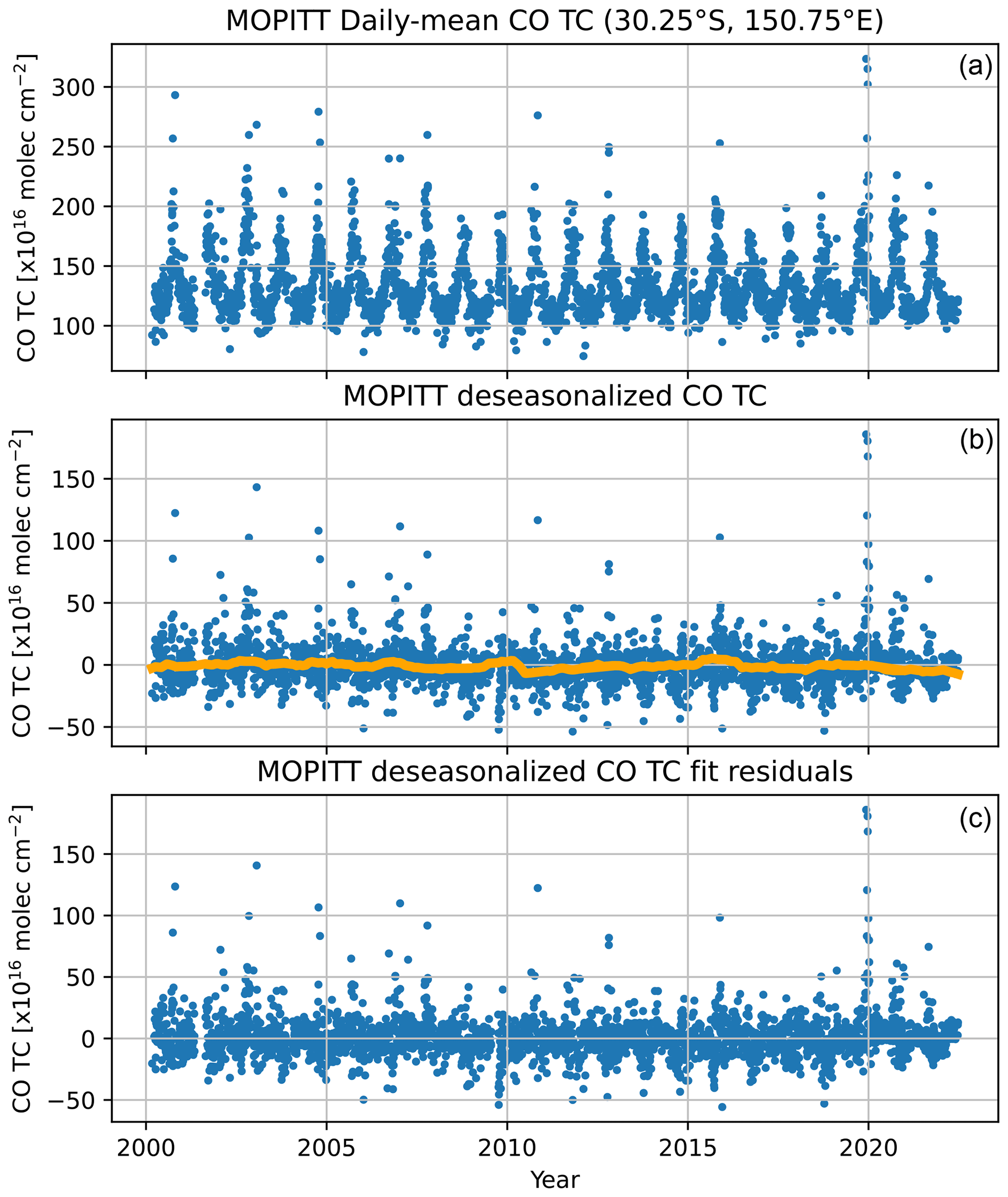
Figure 1Time series of MOPITT daily-mean CO total column (TC; in 1016 molec. cm−2) between 3 March 2000 and 31 July 2022 (a) as well as the deseasonalized time series and the regression fit of the deseasonalized time series (b; blue dots represent the time series and the orange line represents the fit). The MEI term in the regression is included to account for the influence of the ENSO. Fit coefficients were determined for this grid cell as a0=228.7, at=0.11, and aMEI=2.74. The residuals from this fit, used to identify episodic emission events, are shown in panel (c). Data are shown for a 0.5 by 0.5° grid cell centred over land in New South Wales, Australia (grid box centre at 30.25° S, 150.75° E).
After the coefficients of the regression model are determined from MLR, the residuals from the fit are calculated for each grid cell, as shown in the bottom panel of Fig. 1. These residuals are partitioned into discrete histogram bins, using the Freedman–Diaconis method to determine the bin width according to the following equation:
where IQR(r) is the interquartile range of the residual data r and N is the number of observations (Freedman and Diaconis, 1981). As a result of the differences in the interquartile range and the number of observations available in each 0.5 by 0.5° grid cell, the histogram bin width of each grid cell varies. This method is employed as it minimizes the difference between the generated histogram and the shape of the theoretical probability density function (PDF) that underlies the data (Freedman and Diaconis, 1981). It is crucial to note that the residuals cannot be assumed to be characterized by a unimodal Gaussian distribution, as illustrated in Fig. 2.
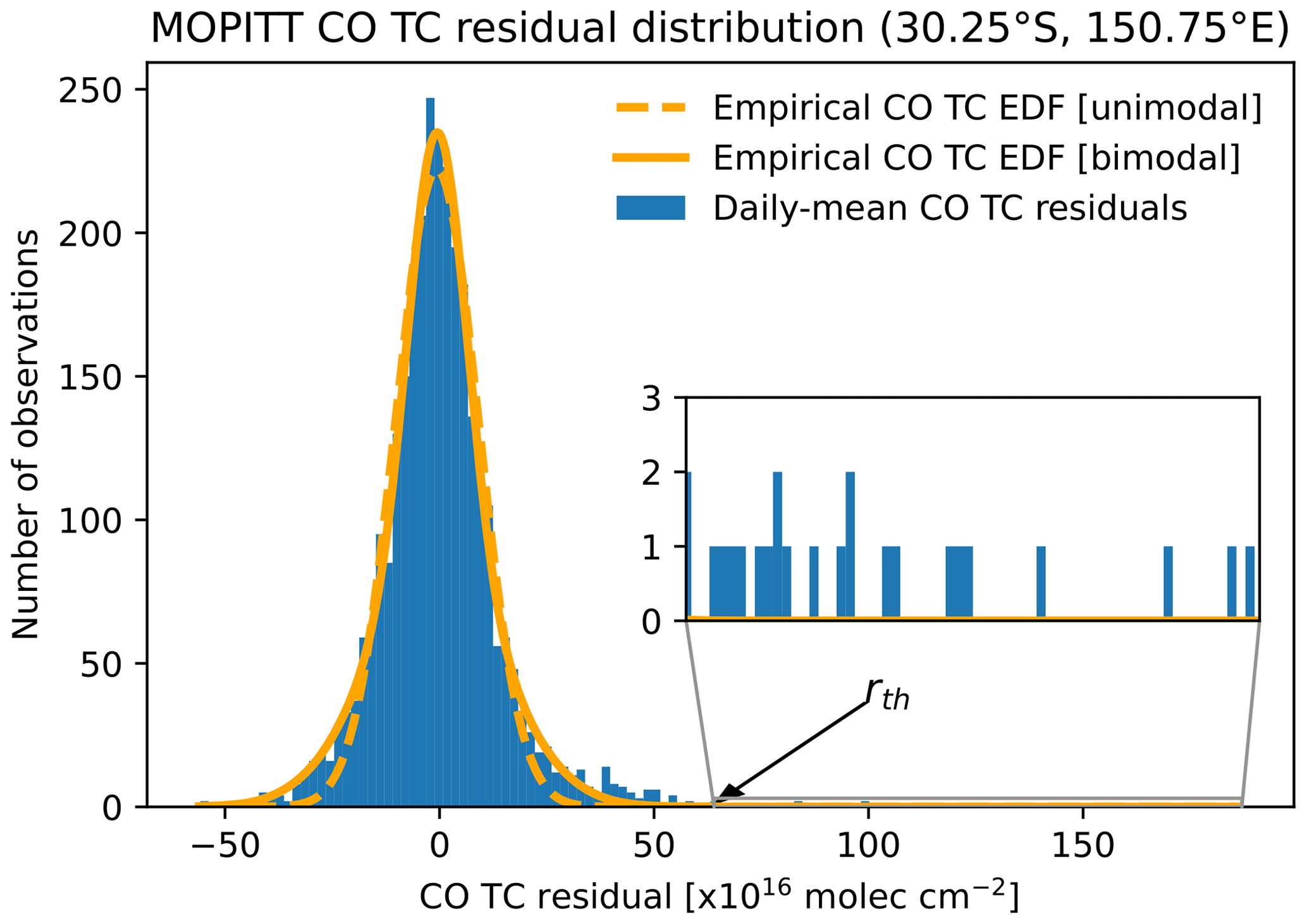
Figure 2MOPITT daily-mean CO total column (TC) residuals, partitioned into discrete histogram bins using the Freedman–Diaconis method (blue bars), and the empirically fitted expectation density functions (EDFs; orange lines) tested. For the grid cell shown, the interquartile range is 14.11×10¹⁶ molec. cm−2, and there were 3015 observations, resulting in a histogram bin width of 1.95×10¹⁶ molec. cm−2. The residuals are fit with both a unimodal (dashed orange line) and bimodal (solid orange line) Gaussian distribution, with the latter having been found to yield the better estimate of the EDF for this grid cell as per the reduced χ2 metric. Note the extended wings of the residual distribution that necessitate a bimodal Gaussian to properly capture the behaviour of the underlying EDF. The black arrow indicates the threshold value (rth) for this grid cell, of 63×1016 molec. cm−2, and the inset shows a magnified view of the data found to be above this threshold value. Data are shown for a 0.5 by 0.5° grid cell centred over land in New South Wales, Australia (grid box centre at 30.25° S, 150.75° E), and they cover the period 3 March 2000 to 31 July 2022.
Once the histogram of the residual data is generated, the methods adapted from Sheese et al. (2015) for screening for outlier data, which explicitly do not assume symmetric or unimodal Gaussian characteristics for the data, can be applied. This process involves analyzing the expectation density function (EDF) of the data, represented by
which is equal to the normalized probability density function (PDF) of the data multiplied by the number of data points, N. The integral of the EDF over all space is equal to the total number of data points observed, and the integral between any two values gives the number of observations expected in that range. As noted in Sheese et al. (2015), this latter property allows for the identification of threshold values, rth, the integral from which to infinity would evaluate to some tolerance level as given by
This is similar in application to both Pierce's criterion and Chauvenet's criterion; however, this approach does not necessitate that the data are normally distributed (Sheese et al., 2015). It is through the identification of these threshold values that observations potentially affected by episodic emission events can be identified.
Given the aforementioned property of the threshold values, the criteria for detecting episodic emission events then become those events whose residuals are larger than the threshold value for a given grid cell, indicative that those are the points with very low probability of occurring given the expected behaviour outlined in the regression model. The tolerance level is chosen to be 0.05, corresponding to a 95 % confidence that the outlier values correspond to irregular emission events (Sheese et al., 2015). This method requires an analytical estimate of the EDF for each grid cell, which is found by empirically fitting the histogram of the residual data using a unimodal and bimodal Gaussian distribution in order to account for any asymmetry or non-Gaussian features in the distribution. The reduced χ2 metric is calculated for each fit and used to evaluate the goodness of fit for both fits of each grid cell. The fit with the better reduced χ2 value is used as the estimate of the EDF. An example of a unimodal and bimodal fit is shown in Fig. 2, with the latter having been found to be the better fit, as per the reduced χ2 metric, for the grid cell shown. From this, the threshold values are identified by evaluating the integral in Eq. (4) over a range of values for rth until the threshold value is found that satisfies the tolerance level. Values outside of the threshold range are flagged as those being potentially affected by episodic emission events, and the results are used to produce a set of enhancement flag files, which contain the location and time information for these flagged daily-mean observations along with the threshold value for the grid cell in which the enhancement occurs and the daily-mean CO total column and measurement error for the anomaly event.
To illustrate the results of this methodology, the measurements that are flagged as those affected by episodic events from the example time series and residual histogram shown in Figs. 1 and 2 can be explored in detail. Integration of the empirically derived estimate of the EDF for this particular grid cell (centred over 30.25° S, 150.75° E; over land in New South Wales, Australia) determined the threshold value for the deseasonalized time series to be 63×1016 molec. cm−2. Given this threshold, 24 daily-mean observations are identified as statistically unlikely to have arisen, given the EDF, without the influence of an episodic CO emission event. Of these 24 observations, 7 correspond to the 2019–2020 Australia Black Summer bushfires which were some of the largest biomass-burning events on record for New South Wales (Davey and Sarre, 2020). Outside of these days, five further observations are found to be coincident with other major Australian bushfires. These events include one on 23 January 2002, around the time of the Black Christmas bushfires; one on 7 November 2002, near the end of the 2002 Victoria wildfires; one on 24 January 2003, at the end of the Canberra bushfires; and a pair on 23 September 2006 and 13 January 2007 that align with the 2006–2007 Australian bushfire season. However, half of the observations flagged as those influenced by episodic emission events do not directly correspond to known major biomass-burning events in the region. Furthermore, not all known major burning events lead to observations that are flagged using this method. This underpins one of the key strengths of the detection algorithm outlined in this work, which is that it is agnostic toward prior assumptions of the impact various events can have on the MOPITT L2 data. This selective flagging allows for an extremely robust approach to data handling that maximizes the amount of information available for analysis, as it does not flag events which do not impact the CO time series in a significant manner.
Examining the global dataset, the MOPITT episodic event threshold values are shown in Fig. 3, while Fig. 4 shows the global distribution of enhancement flags for the daily-mean observations in the gridded L2 dataset. Beginning with the threshold values in Fig. 3, the highest threshold values are found in central South America, Indonesia, western Africa, and eastern China. Given that the seasonality and contributions from the ENSO are explicitly accounted for in the emission event algorithm, the sources of the high thresholds in these cases are frequent large CO emissions with high year-to-year variability. This leads the underlying EDFs of these regions to be very broad and results in there being few enhancement events observed where there are these high thresholds. The lack of flagging for these regions indicates that the method is functioning as it should, only highlighting daily-mean observations that are statistically unlikely to arise. This is exemplified in South America where frequent emission events are found to occur in this region, as shown in Fig. 4. In this example, little overlap is found between where the high threshold values are observed and where the flagged emission events occur, with the latter being located to the east of the former. This pattern also emphasizes the role of transport in enhancing the CO total column on a global basis, and it illustrates the potential for the separation of CO sources and the regions which they might impact.
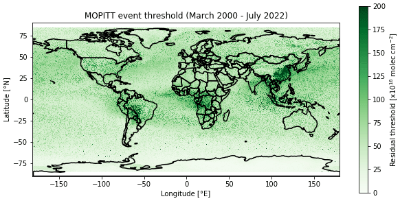
Figure 3MOPITT deseasonalized time series of episodic event threshold values. Data are shown on a 0.5 by 0.5° grid and cover the period 3 March 2000 to 31 July 2022.
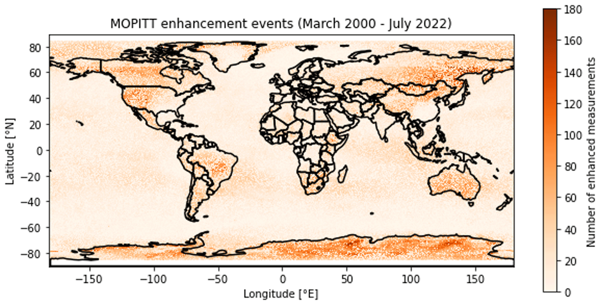
Figure 4Distribution and number of days in the MOPITT L2 daily-mean measurement dataset that are flagged as having been affected by episodic CO emission events. Data are shown on a 0.5 by 0.5° grid and cover the period 3 March 2000 to 31 July 2022.
From the analysis of the four regions with the highest threshold values, the source of the observed threshold values in each is found to vary. The high threshold values over central South America appear to be associated with the frequent wildfires and deforestation in the Amazon, those over Indonesia with the biomass burning during the Indonesian dry season, those over western Africa with agricultural fires in sub-Saharan Africa, and those over eastern China with widespread industrial activity and irregular annual variation in CO emissions. Within these four regions, the CO sources are associated, to at least some degree, with human activity and directly contribute to the interannual variation in these emission sources. However, these sources are captured by the broad EDFs of these regions, implying a predictable behaviour with few events that arise outside of the expected behaviour.
Figure 4, which shows the distribution of enhancement flags, exhibits several regions that display notably higher concentrations of episodic events than the rest of the world: namely western North America (Canada and the United States), the Amazon (Brazil), northeast Asia (Siberia), Australia, and Antarctica. The first four of these experience semi-frequent large CO-emitting wildfires that occur on a variable, nonseasonal basis. Their variable and sporadic nature identifies these events as outliers.
In contrast, the high concentration of outlier events over Antarctica is thought to arise because of CO transport. As there are few emission sources of CO in Antarctica, the CO total column over Antarctica is typically much less than the global average and very stable with little interannual variability. As a result, a relatively small quantity of CO, transported from emission sources elsewhere in the world, can greatly enhance the CO total column, leading observations to be flagged as being associated with an emission event. This property is shown in Fig. 3, which shows that the episodic event threshold values over Antarctica are among the lowest in the world, and small enhancements are likely to be flagged as outliers. Altogether, the combination of the enhancement flags with the event thresholds enables a condensed examination of what can be considered the typical behaviour of CO total columns on a global basis.
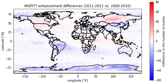
Figure 5Differences in the number of enhancement events identified in the MOPITT L2 daily-mean measurements between two periods corresponding to the measurements made between 3 March 2000 and 31 December 2010 and those made between 1 January 2011 and 31 December 2021.
The temporal distribution of the flagged observations in each grid cell can also be analyzed in order to identify changes in the frequency of enhancement events over time. While the sporadic nature of these enhancement events obfuscates the detection of trends when considering the evolution in the number of these events between individual years, examining multiyear periods allows for an overview of their change with time. To this end, the episodic emission events identified, shown in Fig. 4, have been separated into two periods of roughly equal length, corresponding to the MOPITT measurements made between 3 March 2000 and 31 December 2010 and those made between 1 January 2011 and 31 December 2021. The difference in the number of events in each of these two periods can then be readily calculated as the number of enhancement events in latter period minus those in the former. The results of this are shown in Fig. 5, and from this plot several key features arise. Immediately evident is a small overall trend toward fewer enhancement events over most of the globe in the latter portion of the MOPITT measurement dataset, with the largest decreases happening over Antarctica. However, North America, Siberia, and the eastern coast of Africa all show increasing numbers of enhancement events. Addressing first the general global decrease in the number of events, while the exact cause of this general decrease is uncertain, we found that there is a high likelihood that this decrease is correlated with the decrease in global CO emissions over the MOPITT measurement period (Worden et al., 2013a; Hedelius et al., 2021). The global decrease in CO emissions would also likely reduce the number of observed enhancement events over Antarctica, which are transport-dependent in nature and thus strongly influenced by emissions elsewhere. In contrast to this, the regions displaying elevated numbers of enhancement events in the latter period are most likely affected by an increase in fire frequency and intensity associated with anthropogenic climate change (Dutta et al., 2016; Hart et al., 2019; Saito et al., 2022). Altogether, these findings indicate that the enhancement flags can also aid in understanding the changes in the behaviour of the CO total column over time on a global basis.
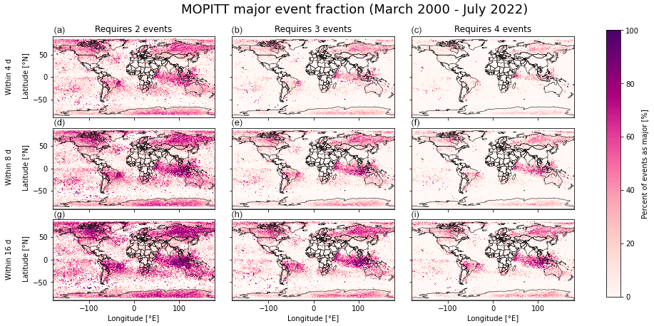
Figure 6Fraction of flagged observations in the MOPITT L2 daily-mean measurement dataset associated with major emission events using nine different classification criteria. Major events consist of those events with two, three, or four flagged observations in a grid cell within at most 4, 8, or 16 d of each other. The columns correspond to the number of required observations: two (a, d, g), three (b, e, h), or four (c, f, i). The rows correspond to the maximum length of time between daily-mean observations for them to be considered part of the same event: 4 d (a, b, c), 8 d (d, e, f), or 16 d (g, h, i). Data are shown on a 0.5 by 0.5° grid and cover the period 3 March 2000 to 31 July 2022.
These enhancement flags can also be used to estimate the fraction of flagged observations in each grid cell associated with major enhancement events by linking flagged measurements based on their temporal distribution. For this purpose, two main factors need to be considered: the number of flagged observations required for an enhancement event to be considered a major event (clustering) and the maximum amount of time between flagged observations for them to still be considered linked (persistence). Naturally, the selection of these factors would impact the frequency and distribution of major enhancement events; however, the response to either of these factors in the number of these major events in any grid cell is influenced by the unique distribution of flagged observations in each cell.
To explore this, a set of nine classification criteria have been examined using three different values for the choice of the time frame for which observations can be considered linked and three values for the number of observations required for an event to be considered a major event. For the former, flagged observations are considered linked if they are within at most 4, 8, or 16 d of each other, with all further observations within a rolling window of that same period treated as part of the same event, while for the latter, at least two, three, or four flagged observations are required for an event to be considered major. Figure 6 shows the fraction of flagged daily-mean observations associated with major enhancement events for each of the criteria permutations tested. As expected, clustering generally increases with the time window permitted between flagged observations for an event and persistence decreases with the number of linked observations in the window. However, not all areas are impacted equally by each change in criteria. This property can be exploited to investigate major enhancement events by analyzing their responses to different criteria.
Here we focus briefly on five regions in Fig. 6 that show that a majority of their flagged observations are associated with major enhancement events under multiple classification criteria. These five regions roughly correspond to northern North America (Canada and Alaska), Siberia, the Amazon (Brazil and the western Atlantic Ocean), the east coast of equatorial Africa, and the equatorial Indian Ocean including Indonesia. Antarctica is excluded from discussion here due to the ease with which transport can dramatically enhance the CO column, as discussed above. Across these five regions, increasing clustering or decreasing persistence causes a gradual reduction in major-event fractions.
In northern North America and Siberia, there are moderate episodic event thresholds (Fig. 3), fairly frequent enhancement events (Fig. 4), and a reduction in the major-event fraction (Fig. 6) with increasing clustering or persistence requirements for major-event classification. Together, this implies that the major events over these two regions are sporadic and likely originate within the regions themselves. As a result, it is found that increasing the stringency of the major-event classification criteria deemphasizes transport processes, restricting the area within each region displaying high major-event fractions to those areas most likely containing the direct CO emission source(s).
The Amazon shows the relationship between transport from emission sources and high major emission event fractions. In the central Amazon, high event thresholds indicate the presence of large, frequent CO emission sources. The eastward propagation of CO from these sources leads to the numerous enhancement events observed over western Brazil and the high major-event fractions seen over Brazil and the western Atlantic Ocean. Elevated episodic event thresholds and major-event fractions are also found drifting across the Atlantic Ocean to the coast of Africa, indicative of the far-reaching effects of transport from these emission sources.
The eastern coast of equatorial Africa shows significantly different behaviour than the prior regions. High episodic event thresholds, shown in Fig. 3, are observed over central Africa, extending westward out over the eastern Atlantic Ocean; however, there are very few enhancement events, as shown in Fig. 4, and very low major-event fractions over this region. This implies a very regular annual cycle in CO emissions with few deviations. The exception to the low major-event fractions occurs off the eastern coast of Africa, an area for which these fractions display high persistence and clustering. As transport from central Africa appears to be predominately westward, evidenced by the drift in high threshold values over the Atlantic, the high major-event fractions off of the eastern coast are likely the result of instances of eastward transport carrying large CO plumes out over a region with comparatively few regular emissions.
The equatorial Indian Ocean also displays significantly different patterns than the previous regions. Around Indonesia, very high episodic event thresholds are found, and few enhancement events are observed across the whole region. However, the high persistence and clustering shown by the major-event fractions, stretching from Indonesia across the Indian Ocean toward the west coast of Africa, imply the existence of occasional extreme events. Thus, the likely source of the most significant deviations in CO behaviour for this entire region stems from the westward transport of CO emissions from these extreme events.
Altogether, by combining the number of flagged observations from Fig. 4 with the major-event information from Fig. 6, a thorough exploration of the types of events identified in this study can be undertaken. From these examples, it is evident that the utility of the MOPITT enhancement flags extends beyond identifying enhancement events and into classifying groupings of these enhancements. Furthermore, grouping enhancement events to identify major events also facilitates analyses of major CO emission events on a global scale by readily identifying major events and their properties.
Motivated by the need for an improved understanding of CO, this study developed a multistep algorithm to detect days in the L2 MOPITT CO dataset that had been affected by large episodic CO emission events. This process involves deseasonalizing an observed total column time series with a centred moving average, fitting the deseasonalized time series with an empirical model of CO trends and periodic drivers, and then fitting the resulting residuals with multimodal Gaussian distributions to estimate the EDFs of the data. This latter step, which adapts the work of Sheese et al. (2015) for detecting outliers in the ACE-FTS measurement dataset, allows for threshold values to be empirically defined, the data above which correspond to observations influenced by episodic emission events. Using these methods, the 22-year MOPITT L2 CO data record has been screened for these events, and enhancement flag files have been produced that identify corresponding days. Overall, these enhancement flags, coupled with the extensive 22-year MOPITT data record, provide insight into the distribution and frequency of these large episodic emission events and can enable more robust approaches for a wide array of applications, such as measurement validation and CO modelling, by carefully screening the data before use.
MOPITT Level 2 data are available from https://doi.org/10.5067/TERRA/MOPITT/MOP02T.009 (MOPITT, 2022). The MOPITT enhancement event flags developed as a part of this study are available from https://doi.org/10.5683/SP3/UU5I7Z (Jeffery and Walker, 2023).
This study was designed by PSJ with input from JRD, JZ, and KAW. PSJ wrote the manuscript and performed the analyses. JRD and JZ provided their expertise on MOPITT. KAW provided insight into the expectation density functions used with ACE-FTS. Valuable comments on the manuscript were provided by all authors.
The authors declare that they have no conflict of interest.
Publisher’s note: Copernicus Publications remains neutral with regard to jurisdictional claims made in the text, published maps, institutional affiliations, or any other geographical representation in this paper. While Copernicus Publications makes every effort to include appropriate place names, the final responsibility lies with the authors.
The authors would like to thank the CSA (Canadian Space Agency) for their financial support of this research. The authors would also like to thank Patrick Sheese, whose work on detecting ACE-FTS outliers laid important groundwork that could be built upon for this study. NCAR (National Center for Atmospheric Research) is sponsored by the National Science Foundation and operated by the University Corporation for Atmospheric Research. The NCAR MOPITT project is supported by the National Aeronautics and Space Administration (NASA) Earth Observing System (EOS) program. The MOPITT team acknowledges support from the Canadian Space Agency (CSA), the Natural Sciences and Engineering Research Council of Canada (NSERC), and Environment and Climate Change Canada (ECCC) and the contributions of COMDEV and ABB Bomem.
This research has been supported by the Canadian Space Agency (grant no. 9F045-170863/001/MTB).
This paper was edited by Bryan N. Duncan and reviewed by Shyno Susan John and one anonymous referee.
Brenninkmeijer, C. A. M., Röckmann, T., Bräunlich, M., Jöckel, P., and Bergamaschi, P.: Review of progress in isotope studies of atmospheric carbon monoxide, Chemosphere, 1, 33–52, https://doi.org/10.1016/S1465-9972(99)00018-5, 1999. a, b
Buchholz, R. R., Worden, H. M., Park, M., Francis, G., Deeter, M. N., Edwards, D. P., Emmons, L. K., Gaubert, B., Gille, J., Martínez-Alonso, S., Tang, W., Kumar, R., Drummond, J. R., Clerbaux, C., George, M., Coheur, P.-F., Hurtmans, D., Bowman, K. W., Luo, M., Payne, V. H., Worden, J. R., Chin, M., Levy, R. C., Warner, J., Wei, Z., and Kulawik, S. S.: Air pollution trends measured from Terra: CO and AOD over industrial, fire-prone, and background regions, Remote Sens. Environ., 256, 112275, https://doi.org/10.1016/j.rse.2020.112275, 2021. a
Buchholz, R. R., Park, M., Worden, H. M., Tang, W., Edwards, D. P., Gaubert, B., Deeter, M. N., Sullivan, T., Ru, M., Chin, M., Levy, R. C., Zheng, B., and Magzamen, S.: New seasonal pattern of pollution emerges from changing North American wildfires, Nat. Commun., 13, 2043, https://doi.org/10.1038/s41467-022-29623-8, 2022. a
Dasari, S., Andersson, A., Popa, M. E., Röckmann, T., Holmstrand, H., Budhavant, K., and Gustafsson, O.: Observational Evidence of Large Contribution from Primary Sources for Carbon Monoxide in the South Asian Outflow, Environ. Sci. Technol., 56, 165–174, https://doi.org/10.1021/acs.est.1c05486, 2022. a
Davey, S. M. and Sarre, A.: Editorial: the 2019/20 Black Summer bushfires, Aust. Forestry, 83, 47–51, https://doi.org/10.1080/00049158.2020.1769899, 2020. a
Deeter, M., Francis, G., Gille, J., Mao, D., Martínez-Alonso, S., Worden, H., Ziskin, D., Drummond, J., Commane, R., Diskin, G., and McKain, K.: The MOPITT Version 9 CO product: sampling enhancements and validation, Atmos. Meas. Tech., 15, 2325–2344, https://doi.org/10.5194/amt-15-2325-2022, 2022. a, b, c, d, e, f, g
Deeter, M. N., Emmons, L. K., Francis, G. L., Edwards, D. P., Gille, J. C., Warner, J. X., Khattatov, B., Ziskin, D., Lamarque, J.-F., Ho, S.-P., Yudin, V., Attié, J.-L., Packman, D., Chen, J., Mao, D., and Drummond, J. R.: Operational carbon monoxide retrieval algorithm and selected results for the MOPITT instrument, J. Geophys. Res.-Atmos., 108, 4399, https://doi.org/10.1029/2002JD003186, 2003. a
Deeter, M. N., Edwards, D. P., and Gille, J. C.: Retrievals of carbon monoxide profiles from MOPITT observations using lognormal a priori statistics, J. Geophys. Res.-Atmos., 112, D11311, https://doi.org/10.1029/2006JD007999, 2007. a
Deeter, M. N., Edwards, D. P., Gille, J. C., and Drummond, J. R.: CO retrievals based on MOPITT near-infrared observations, J. Geophys. Res.-Atmos., 114, D04303, https://doi.org/10.1029/2008JD010872, 2009. a
Deeter, M. N., Martínez-Alonso, S., Edwards, D. P., Emmons, L. K., Gille, J. C., Worden, H. M., Pittman, J. V., Daube, B. C., and Wofsy, S. C.: Validation of MOPITT Version 5 thermal-infrared, near-infrared, and multispectral carbon monoxide profile retrievals for 2000–2011, J. Geophys. Res.-Atmos., 118, 6710–6725, https://doi.org/10.1002/jgrd.50272, 2013. a, b
Deeter, M. N., Edwards, D. P., Francis, G. L., Gille, J. C., Martínez-Alonso, S., Worden, H. M., and Sweeney, C.: A climate-scale satellite record for carbon monoxide: the MOPITT Version 7 product, Atmos. Meas. Tech., 10, 2533–2555, https://doi.org/10.5194/amt-10-2533-2017, 2017. a, b
Deeter, M. N., Edwards, D. P., Francis, G. L., Gille, J. C., Mao, D., Martínez-Alonso, S., Worden, H. M., Ziskin, D., and Andreae, M. O.: Radiance-based retrieval bias mitigation for the MOPITT instrument: the version 8 product, Atmos. Meas. Tech., 12, 4561–4580, https://doi.org/10.5194/amt-12-4561-2019, 2019. a
Desservettaz, M. J., Fisher, J. A., Luhar, A. K., Woodhouse, M. T., Bukosa, B., Buchholz, R., Wiedinmyer, C., Griffith, D. W. T., Krummel, P. B., Jones, N. B., Deutscher, N. M., and Greenslade, J. W.: Australian Fire Emissions of Carbon Monoxide Estimated by Global Biomass Burning Inventories: Variability and Observational Constraints, J. Geophys. Res.-Atmos., 127, e2021JD035925, https://doi.org/10.1029/2021JD035925, 2022. a
Drummond, J. R., Zou, J., Nichitiu, F., Kar, J., Deschambaut, R., and Hackett, J.: A review of 9-year performance and operation of the MOPITT instrument, Adv. Space Res., 45, 760–774, https://doi.org/10.1016/j.asr.2009.11.019, 2010. a, b
Drummond, J. R., Vaziri Zanjani, Z., F., N., and Zou, J.: A 20-year review of the performance and operation of the MOPITT instrument, Adv. Space Res., 70, 3078–3091, https://doi.org/10.1016/j.asr.2022.09.010, 2022. a, b, c
Dutta, R., Das, A., and Aryal, J.: Big data integration shows Australian bush-fire frequency is increasing significantly, Roy. Soc. Open. Sci., 3, 150241, https://doi.org/10.1098/rsos.150241, 2016. a, b
Edwards, D. P., Halvorson, C. M., and Gille, J. C.: Radiative transfer modeling for the EOS Terra satellite Measurement of Pollution in the Troposphere (MOPITT) instrument, J. Geophys. Res.-Atmos., 104, 16755–16775, https://doi.org/10.1029/1999JD900167, 1999. a
Freedman, D. and Diaconis, P.: On the histogram as a density estimator: L2 theory, Z. Wahrscheinlichkeit, 57, 453–476, https://doi.org/10.1007/BF01025868, 1981. a, b
Gelaro, R., McCarty, W., Suárez, M. J., Todling, R., Molod, A., Takacs, L., Randles, C. A., Darmenov, A., Bosilovich, M. G., Reichle, R., Wargan, K., Coy, L., Cullather, R., Draper, C., Akella, S., Buchard, V., Conaty, A., da Silva, A. M., Gu, W., Kim, G.-K., Koster, R., Lucchesi, R., Merkova, D., Nielsen, J. E., Partyka, G., Pawson, S., Putman, W., Rienecker, M., Schubert, S. D., Sienkiewicz, M., and Zhao, B.: The Modern-Era Retrospective Analysis for Research and Applications, version 2 (MERRA-2), J. Climate, 30, 5419–5454, https://doi.org/10.1175/JCLI-D-16-0758.1, 2017. a
Granier, C., Bessagnet, B., Bond, T., D’Angiola, A., Denier van der Gon, H., Frost, G. J., Heil, A., Kaiser, J. W., Kinne, S., Klimont, Z., Kloster, S., Lamarque, J.-F., Liousse, C., Masui, T., Meleux, F., Mieville, A., Ohara, T., Raut, J.-C., Riahi, K., Schultz, M. G., Smith, S. J., Thompson, A., van Aardenne, J., van der Werf, G. R., and van Vuuren, D. P.: Evolution of anthropogenic and biomass burning emissions of air pollutants at global and regional scales during the 1980–2010 period, Clim. Change, 109, 163, https://doi.org/10.1007/s10584-011-0154-1, 2011. a, b
Hart, S. J., Henkelman, J., McLoughlin, P. D., Nielsen, S. E., Truchon-Savard, A., and Johnstone, J. F.: Examining forest resilience to changing fire frequency in a fire-prone region of boreal forest, Glob. Change Biol., 25, 869–884, https://doi.org/10.1111/gcb.14550, 2019. a, b
Hedelius, J. K., Toon, G. C., Buchholz, R. R., Iraci, L. T., Podolske, J. R., Roehl, C. M., Wennberg, P. O., Worden, H. M., and Wunch, D.: Regional and Urban Column CO Trends and Anomalies as Observed by MOPITT Over 16 Years, J. Geophys. Res.-Atmos., 126, e2020JD033967, https://doi.org/10.1029/2020JD033967, 2021. a, b, c, d, e
Jeffery, P. and Walker, K.: MOPITT V9 TIR Anomaly Event Flags, Version V1, Borealis [data set], https://doi.org/10.5683/SP3/UU5I7Z, 2023. a
Jiang, Z., Worden, J. R., Worden, H., Deeter, M., Jones, D. B. A., Arellano, A. F., and Henze, D. K.: A 15-year record of CO emissions constrained by MOPITT CO observations, Atmos. Chem. Phys., 17, 4565–4583, https://doi.org/10.5194/acp-17-4565-2017, 2017. a, b
John, S. S., Deutscher, N. M., Paton-Walsh, C., Velazco, V. A., Jones, N. B., and Griffith, D. W. T.: 2019–20 Australian Bushfires and Anomalies in Carbon Monoxide Surface and Column Measurements, Atmosphere, 12, 755, https://doi.org/10.3390/atmos12060755, 2021. a
Khalil, M. A. K. and Rasmussen, R. A.: Global decrease in atmospheric carbon monoxide concentration, Nature, 370, 639–641, https://doi.org/10.1038/370639a0, 1994. a
Lamarque, J.-F., Emmons, L. K., Hess, P. G., Kinnison, D. E., Tilmes, S., Vitt, F., Heald, C. L., Holland, E. A., Lauritzen, P. H., Neu, J., Orlando, J. J., Rasch, P. J., and Tyndall, G. K.: CAM-chem: description and evaluation of interactive atmospheric chemistry in the Community Earth System Model, Geosci. Model Dev., 5, 369–411, https://doi.org/10.5194/gmd-5-369-2012, 2012. a
Lelieveld, J., Gromov, S., Pozzer, A., and Taraborrelli, D.: Global tropospheric hydroxyl distribution, budget and reactivity, Atmos. Chem. Phys., 16, 12477–12493, https://doi.org/10.5194/acp-16-12477-2016, 2016. a, b
MOPITT: MOPITT Version 9 Level 2 Data, Atmospheric Science Data Center [data set], https://doi.org/10.5067/TERRA/MOPITT/MOP02T.009, 2022. a
Park, M., Worden, H. M., Kinnison, D. E., Gaubert, B., Tilmes, S., Emmons, L. K., Santee, M. L., Froidevaux, L., and Boone, C.: Fate of Pollution Emitted During the 2015 Indonesian Fire Season, J. Geophys. Res.-Atmos., 126, e2020JD033474, https://doi.org/10.1029/2020JD033474, 2021. a
Petrenko, V. V., Martinerie, P., Novelli, P., Etheridge, D. M., Levin, I., Wang, Z., Blunier, T., Chappellaz, J., Kaiser, J., Lang, P., Steele, L. P., Hammer, S., Mak, J., Langenfelds, R. L., Schwander, J., Severinghaus, J. P., Witrant, E., Petron, G., Battle, M. O., Forster, G., Sturges, W. T., Lamarque, J.-F., Steffen, K., and White, J. W. C.: A 60 yr record of atmospheric carbon monoxide reconstructed from Greenland firn air, Atmos. Chem. Phys., 13, 7567–7585, https://doi.org/10.5194/acp-13-7567-2013, 2013. a
Qu, Z., Henze, D. K., Worden, H. M., Jiang, Z., Gaubert, B., Theys, N., and Wang, W.: Sector-Based Top-Down Estimates of NOx, SO2, and CO Emissions in East Asia, Geophys. Res. Lett., 49, e2021GL096009, https://doi.org/10.1029/2021GL096009, 2022. a
Saito, M., Shiraishi, T., Hirata, R., Niwa, Y., Saito, K., Steinbacher, M., Worthy, D., and Matsunaga, T.: Sensitivity of biomass burning emissions estimates to land surface information, Biogeosciences, 19, 2059–2078, https://doi.org/10.5194/bg-19-2059-2022, 2022. a, b, c, d, e
Seiler, W. and Crutzen, P. J.: Estimates of gross and net fluxes of carbon between the biosphere and the atmosphere from biomass burning, Clim. Change, 2, 207–247, https://doi.org/10.1007/BF00137988, 1980. a
Seinfeld, J. H. and Pandis, S. N.: Atmospheric chemistry and physics: From air pollution to climate change, Wiley, Hoboken, N.J, 2nd Edn., ISBN 0-471-72017-8, 2006. a
Sheese, P. E., Boone, C. D., and Walker, K. A.: Detecting physically unrealistic outliers in ACE-FTS atmospheric measurements, Atmos. Meas. Tech., 8, 741–750, https://doi.org/10.5194/amt-8-741-2015, 2015. a, b, c, d, e, f
Strode, S. A. and Pawson, S.: Detection of carbon monoxide trends in the presence of interannual variability, J. Geophys. Res.-Atmos., 118, 12257–12273, https://doi.org/10.1002/2013JD020258, 2013. a
Stroud, C. A., Zaganescu, C., Chen, J., McLinden, C. A., Zhang, J., and Wang, D.: Toxic volatile organic air pollutants across Canada: multi-year concentration trends, regional air quality modelling and source apportionment, J. Atmos. Chem, 73, 137–164, https://doi.org/10.1007/s10874-015-9319-z, 2016. a
Wang, Z., Chappellaz, J., Martinerie, P., Park, K., Petrenko, V., Witrant, E., Emmons, L. K., Blunier, T., Brenninkmeijer, C. A. M., and Mak, J. E.: The isotopic record of Northern Hemisphere atmospheric carbon monoxide since 1950: implications for the CO budget, Atmos. Chem. Phys., 12, 4365–4377, https://doi.org/10.5194/acp-12-4365-2012, 2012. a
Worden, H. M., Deeter, M. N., Edwards, D. P., Gille, J. C., Drummond, J. R., and Nédélec, P.: Observations of near-surface carbon monoxide from space using MOPITT multispectral retrievals, J. Geophys. Res.-Atmos., 115, D18314, https://doi.org/10.1029/2010JD014242, 2010. a
Worden, H. M., Deeter, M. N., Frankenberg, C., George, M., Nichitiu, F., Worden, J., Aben, I., Bowman, K. W., Clerbaux, C., Coheur, P. F., de Laat, A. T. J., Detweiler, R., Drummond, J. R., Edwards, D. P., Gille, J. C., Hurtmans, D., Luo, M., Martínez-Alonso, S., Massie, S., Pfister, G., and Warner, J. X.: Decadal record of satellite carbon monoxide observations, Atmos. Chem. Phys., 13, 837–850, https://doi.org/10.5194/acp-13-837-2013, 2013a. a, b, c, d, e, f, g
Worden, J., Jiang, Z., Jones, D. B. A., Alvarado, M., Bowman, K., Frankenberg, C., Kort, E. A., Kulawik, S. S., Lee, M., Liu, J., Payne, V., Wecht, K., and Worden, H.: El Niño, the 2006 Indonesian peat fires, and the distribution of atmospheric methane, Geophys. Res. Lett., 40, 4938–4943, https://doi.org/10.1002/grl.50937, 2013b. a, b
Zhao, Y., Nielsen, C. P., McElroy, M. B., Zhang, L., and Zhang, J.: CO emissions in China: Uncertainties and implications of improved energy efficiency and emission control, Atmos. Environ., 49, 103–113, https://doi.org/10.1016/j.atmosenv.2011.12.015, 2012. a
Zheng, B., Chevallier, F., Yin, Y., Ciais, P., Fortems-Cheiney, A., Deeter, M. N., Parker, R. J., Wang, Y., Worden, H. M., and Zhao, Y.: Global atmospheric carbon monoxide budget 2000–2017 inferred from multi-species atmospheric inversions, Earth Syst. Sci. Data, 11, 1411–1436, https://doi.org/10.5194/essd-11-1411-2019, 2019. a, b, c, d, e, f, g, h