the Creative Commons Attribution 4.0 License.
the Creative Commons Attribution 4.0 License.
 | 23 Feb 2024
An updated modeling framework to simulate Los Angeles air quality – Part 1: Model development, evaluation, and source apportionment
Elyse A. Pennington
Benjamin C. Schulze
Karl M. Seltzer
Jiani Yang
Zhe Jiang
Hongru Shi
Melissa Venecek
Daniel Chau
Benjamin N. Murphy
Christopher M. Kenseth
Ryan X. Ward
Havala O. T. Pye
This study describes a modeling framework, model evaluation, and source apportionment to understand the causes of Los Angeles (LA) air pollution. A few major updates are applied to the Community Multiscale Air Quality (CMAQ) model with a high spatial resolution (1 km × 1 km). The updates include dynamic traffic emissions based on real-time, on-road information and recent emission factors and secondary organic aerosol (SOA) schemes to represent volatile chemical products (VCPs). Meteorology is well predicted compared to ground-based observations, and the emission rates from multiple sources (i.e., on-road, volatile chemical products, area, point, biogenic, and sea spray) are quantified. Evaluation of the CMAQ model shows that ozone is well predicted despite inaccuracies in nitrogen oxide (NOx) predictions. Particle matter (PM) is underpredicted compared to concurrent measurements made with an aerosol mass spectrometer (AMS) in Pasadena. Inorganic aerosol is well predicted, while SOA is underpredicted. Modeled SOA consists of mostly organic nitrates and products from oxidation of alkane-like intermediate volatility organic compounds (IVOCs) and has missing components that behave like less-oxidized oxygenated organic aerosol (LO-OOA). Source apportionment demonstrates that the urban areas of the LA Basin and vicinity are NOx-saturated (VOC-sensitive), with the largest sensitivity of O3 to changes in VOCs in the urban core. Differing oxidative capacities in different regions impact the nonlinear chemistry leading to PM and SOA formation, which is quantified in this study.
- Article
(3912 KB) - Full-text XML
-
Supplement
(5752 KB) - BibTeX
- EndNote


Air quality is influenced by particle- and gas-phase species, which can impact human and environmental health. Particulate matter (PM), or aerosols, affect human health (Lim et al., 2012), climate (Intergovernmental Panel on Climate Change, 2014), and visibility (Hyslop, 2009). A major fraction of PM in urban areas is organic (Zhang et al., 2007), which itself is largely secondary in nature (Jimenez et al., 2009). Secondary organic aerosol (SOA) comprises thousands of species, which are formed via complex chemistry that also produces ozone (O3). O3 is an oxidant which can damage human (Nuvolone et al., 2018) and plant (Sandermann, 1996) health. Reactive organic gases (ROGs) are necessary precursors to these pollutants and span a range of properties, including vapor pressure and the oxygen-to-carbon ratio. Volatile organic compounds (VOCs) and nitrogen oxides (NOx) control O3 and SOA formation, and semivolatile organic compounds (SVOCs) and intermediate volatility organic compounds (IVOCs) have a high potential to form SOA (Robinson et al., 2007).
The Los Angeles Basin has a long history of air pollution, resulting from substantial anthropogenic emissions and unique meteorology. On-road mobile emissions have historically been the most important source of atmospheric pollution in the Los Angeles (LA) Basin, but emissions have decreased as emissions control technologies (i.e., catalytic converters) have improved, vehicle fuel efficiencies have increased, and electric vehicles have become more prevalent (Khare and Gentner, 2018). Other sources of emissions have become more important, particularly VOC and SVOC emissions from volatile chemical products (VCPs). VCPs are consumer and industrial products that utilize evaporative organics (Seltzer et al., 2021) and can form SOA (Qin et al., 2021). Asphalt emissions can also form SOA and are likely important in LA, where the urban land fraction and temperatures are both high (Khare et al., 2020). In addition to organic emission reductions, NOx emissions from on-road vehicles have decreased. Moreover, NOx emissions from off-road vehicles have become almost equally important to on-road NOx emissions in LA (Khare and Gentner, 2018). As total emissions have decreased, ambient levels of most criteria pollutants have decreased, including NOx, carbon monoxide (CO), and sulfur oxides (SOx) (US EPA, 2013). However, O3 in LA has increased over the past decade (US EPA, 2013) because of the nonlinear atmospheric chemistry leading to its formation (Seinfeld and Pandis, 2016; Le et al., 2020). The LA Basin also displays a temperature inversion layer, which leads to strong atmospheric stability with a low-flow rate out of the LA Basin. The complex interactions between emissions, meteorology, and chemistry will be investigated in this study.
Predicting air quality using chemical transport models (CTMs) is challenging. Developing a model that best represents the complexity of atmospheric chemistry – particularly SOA formation – in a reasonable computation time involves a trade-off in chemical detail. Models exist which represent gas-phase and heterogeneous chemistry (e.g., Carter, 2010; Yarwood et al., 2010; Goliff et al., 2013; Keller and Evans, 2019), and researchers have traditionally modeled SOA formation from VOC oxidation (e.g., Odum et al., 1996; Carlton et al., 2010). An active area of research is the oxidation of SVOCs and IVOCs, which likely yield higher SOA than VOCs due to their lower volatility (e.g., Donahue et al., 2011; Murphy et al., 2017; Gentner et al., 2017). It is well documented that SOA tends to be underpredicted in the Community Multiscale Air Quality (CMAQ) model (Appel et al., 2021), unless an empirical representation of anthropogenic SOA is introduced (Murphy et al., 2017), so a goal of model improvement is to increase SOA mass with improved understanding of sources and physiochemical processes. Representing the correct sources of SOA in a process-based approach is critical for model applications designed to inform control strategies. Recent works have developed new models to represent SOA formation from VCPs (Pennington et al., 2021) and mobile sector IVOCs (Lu et al., 2020), which reduced model SOA bias. The predicted chemistry leading to pollutant formation is highly nonlinear (Seinfeld and Pandis, 2016) and is additionally influenced by emission inventories that typically have high uncertainties (Qin et al., 2021; Khare and Gentner, 2018). Recent work has improved the estimation of emission rates of VCP VOCs (Seltzer et al., 2021), on-road VOCs, NOx, PM, and CO (California Air Resources Board, 2018), and on-road IVOCs (Zhao et al., 2016).
Detailed observational data that can be used to constrain model parameters governing chemical transformations is often lacking. While pollutants like O3, PM2.5, and NO2 are regularly monitored throughout the United States of America (US EPA, 2013), these sites tend to be sparsely distributed. Components of PM2.5 are generally only available on a daily integrated basis, thus preventing a diagnostic separation of daytime vs. nighttime chemistry. Measurements of radical species and specific VOCs are only obtained during field campaigns, which are limited to a small region during a short time duration because they are very expensive to carry out. Even though the lack of in situ data makes it difficult to parameterize or evaluate models, it also underscores the importance of models. Models fill in the spatiotemporal gaps in our measurements and allow us to predict important air quality impacts.
The modeling period in this study covers April 2020, during the strict COVID-19 lockdown regulations in LA. On-road vehicle miles traveled (VMT) declined significantly during this month, as many people remained at home (Caltrans, 2020), and this altered the composition of anthropogenic emissions and resulting pollutant levels (Parker et al., 2020). However, this period also experienced several weather patterns that are unusual to the springtime months in LA, namely a rainy period and a very hot period. Untangling the relative impacts of decreased emissions versus meteorology is feasible, using CTMs.
In the first part of this work, we use the CMAQ model to understand the current air quality of the Los Angeles Basin. Model inputs to CMAQ are developed to represent meteorology and emissions in 2020 and are evaluated against available data. CMAQ model predictions are presented throughout the LA Basin, while source apportionment studies describe the important sources of the emissions. SOA formation in Pasadena is compared to detailed ground-based measurements. In Part 2 of this work, currently in preparation, the sensitivity of pollutants to reduced on-road and VCP emissions is further explored. The relative importance of emissions and meteorology in dictating O3 and PM concentrations during the COVID-19 pandemic is also investigated. The simulations investigated in Part 2 can represent future emission scenarios and provide insight into helpful policies to mitigate air quality.
2.1 Model development
The model framework is summarized in Fig. 1, and detailed descriptions of each component are described below. CTM inputs include meteorology, emissions, chemical boundary conditions, and grid information. The CTM uses these inputs to predict concentrations which will be compared to hourly or daily observed data throughout the domain and specifically in Pasadena.
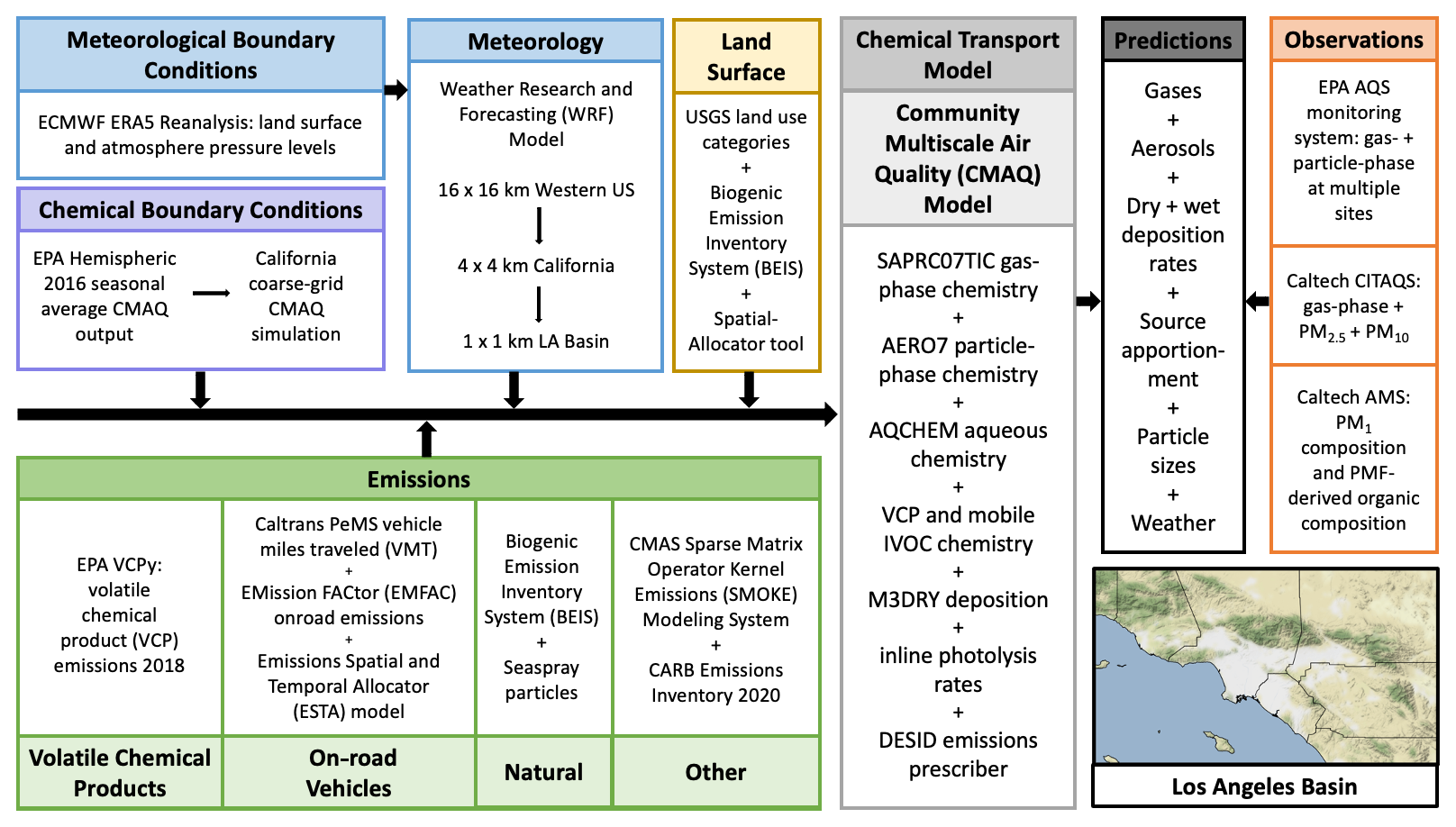
Figure 1Model framework describing the inputs to CMAQ, CMAQ configuration, observational data, and modeling domain.
2.1.1 Chemical transport model
We use CMAQ version 5.3.2 (US EPA Office of Research and Development, 2020), which is documented and evaluated in Appel et al. (2021). The gas-phase chemical mechanism used here is SAPRC07TIC (Carter, 2010; Xie et al., 2013), the organic-aerosol-phase chemical mechanism is AERO7 (Pye et al., 2013, 2017; Murphy et al., 2017; Xu et al., 2018; Qin et al., 2021), the inorganic-aerosol-phase chemical mechanism is ISORROPIA II (Fountoukis and Nenes, 2007), and the aqueous-phase chemical mechanism used is AQCHEM (Fahey et al., 2017). The M3Dry module is the air–surface exchange module used to represent the dry deposition of gas- and particle-phase species (Pleim and Ran, 2011; Appel et al., 2021) and uses the Noah land surface model (Alapaty et al., 2008). The Detailed Emissions Scaling, Isolation, and Diagnostic (DESID) module within CMAQ (Murphy et al., 2021) was used to modify emissions and in our source apportionment sensitivity simulations. The SAPRC07TIC_AE7 chemical mechanism used here was updated to include the emissions and chemistry of VCP species (Pennington et al., 2021) and IVOCs from on-road mobile sources (Lu et al., 2020). The organic aerosol (OA) chemical mechanism is summarized in Fig. S1 in the Supplement.
2.1.2 Meteorology
Meteorological simulations are performed using the Weather Research and Forecasting (WRF) Model (Skamarock et al., 2008) version 4.2. Climatological input data are provided from the ERA5 Reanalysis dataset (Hersbach et al., 2018, p. 5), which contains hourly data on a 0.25° × 0.25° grid at the surface and on 37 pressure levels from 100 to 1 hPa. The WRF configuration uses three nested domains to resample and simulate the meteorological variables from the input resolution to 16, 4, and then 1 km resolution (Fig. 2a). The innermost 1 km × 1 km domain is the region of interest in this study and referred to as the LA domain (Fig. 2a, c).
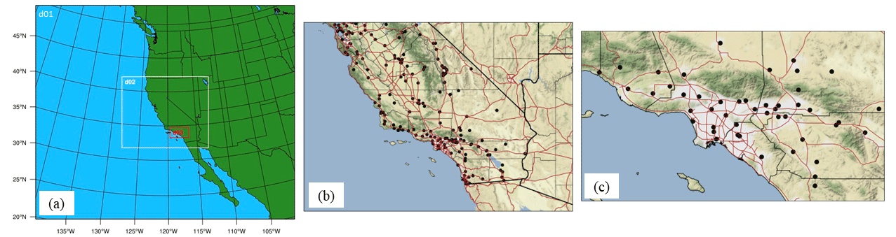
Figure 2(a) Three nested domains used in the WRF simulations. d01 has a horizontal resolution of 16 km, d02 has a resolution of 4 km, and d03 has a resolution of 1 km. (b) California's 4 km × 4 km coarse-resolution domain. (c) LA's 1 km × 1 km fine-resolution domain. Thick black lines are state borders, and thin black lines are county borders. Black dots represent the U.S. Environmental Protection Agency (EPA)'s Air Quality System (AQS) sites and red lines are freeways.
2.1.3 Emissions
On-road vehicles can be separated into two categories, light duty and heavy duty, based on the weight of the vehicle. Light-duty vehicles (LDVs) are smaller, tend to be passenger cars, and tend to use gasoline fuel. On the other hand, heavy-duty vehicles (HDVs) are larger, tend to be used for transport, and tend to use diesel fuel. These categories are represented separately in the model because there has been historical interest in understanding the class of vehicles and fuels to target for emissions regulations (e.g., Bahreini et al., 2012; Ensberg et al., 2014; Gentner et al., 2017; Lu et al., 2020). Additionally, because of the different uses of these types of vehicles, their driving and therefore emissions patterns differ spatially and temporally.
On-road mobile emissions are represented by the EMission FACtor 2017 (EMFAC2017) emissions inventory and model projected to year 2020 (California Air Resources Board, 2018). The projection to year 2020 includes the 2020-specific meteorological effects on emission rates. The Emissions Spatial and Temporal Allocator (ESTA) model uses 1 km × 1 km spatial surrogates and California Vehicle Activity Database (CalVAD) temporal surrogates (Ritchie and Tok, 2016) to calculate hourly, gridded emissions on the LA domain. The speciation profiles used in ESTA include the surrogate NMOGs (non-methane organic gases), which provide diagnostic information but are not used by the chemistry in CMAQ. To estimate emissions of alkane-like IVOC emissions, the unspeciated fraction of NMOGs was used with information from Lu et al. (2020).
EMFAC and ESTA do not capture the effect of COVID-19 on vehicle use, so we modified the on-road emissions to include those changes. The California Performance Measurement System (PeMS) uses in situ detectors distributed throughout California to measure vehicle usage metrics (Caltrans, 2020). One such metric is vehicle miles traveled (VMT), which measures the miles traveled by different vehicle types, e.g., light- and heavy-duty vehicles. The VMT changed directly in response to COVID-19 policies and human behavior changes, so it can be used to reduce on-road emissions in response to the pandemic (Yang et al., 2021). VMT data were summed for all PeMS monitoring sites in the LA domain and separated into heavy-duty and light-duty vehicles (Fig. 3a–b). The VMT for January through March (pre-pandemic) was relatively constant. These values were averaged and used as the baseline VMT, represented by the dashed black lines. The VMT decreased in March as COVID-19 stay-at-home policies were implemented, reached its lowest value in April, and then slowly increased towards the baseline value. All weekly averaged VMT values were divided by the baseline VMT value to obtain scaling factors which are a proxy for declining vehicle emissions resulting from the pandemic (Fig. 3c). The VMT scaling factors are not identical for light-duty and heavy-duty vehicles, which is consistent with the rationale for separating these vehicle types. Light-duty VMT decreased the most, since the pandemic primarily decreased the use of personal vehicles, with a lesser decrease in the use of industrial transport vehicles (i.e., heavy-duty vehicles).
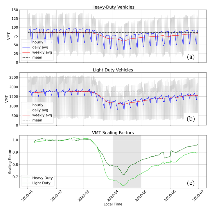
Figure 3Hourly (gray), daily averaged (blue), and weekly averaged (red) VMT data (Caltrans, 2020) for (a) heavy-duty vehicles and (b) light-duty vehicles. The VMT averaged from 1 January–1 March 2020 is represented by the dashed black line. (c) The weekly averaged VMT divided by the January–March mean for heavy-duty (dark green) and light-duty (light green) vehicles. The gray shaded area covers the modeling period from 1–30 April 2020.
VCP emissions are predicted using the VCPy model framework (Seltzer et al., 2021). VCPy version 1.1 (Seltzer et al., 2022) was used to calculate VOC emission rates for 2018 over the contiguous United States (CONUS) on a 4 km × 4 km grid, which were re-gridded to 1 km × 1 km to fit the LA domain grid. The year 2018 emissions are assumed to be representative of the year 2020 emissions within the range of uncertainty present in VCPy.
Natural emissions are treated in-line in CMAQ, using land surface descriptive files generated using the Spatial Allocator tool (US EPA, 2022). Gas-phase biogenic emissions and particle-phase sea spray emissions are modeled using the Biogenic Emission Inventory System (BEIS) version 3.6.1 (Bash et al., 2016). Particle-phase sea spray emissions are modeled according to the method of Gantt et al. (2015). Wildfire emissions were not included, as this time period experienced limited wildfire activity. Lightning NOx and windblown dust emissions are not turned on in the model. Dust makes up a small fraction of total PM loading. Hayes et al. (2013) showed that, in Pasadena, dust makes up only 1.6 % of total PM1 by mass. Natural emissions are the lowest source of PM emissions (CARB, 2020), so windblown dust is a minor contributor to total PM. However, it is possible that muting the dust scheme could cause underestimations of PM2.5 and PM10. Previous work suggests that crustal elements, i.e., dust elements, do not have a large impact on modeled ammonium and nitrate concentrations, so omitting these emissions should not have a large impact on other inorganic aerosol or gas-phase species. Previous work (e.g., Choi et al., 2009) has shown that lightning NOx is nearly negligible over southern California.
All other emissions are calculated using the California Air Resources Board (CARB) emissions inventory (CARB, 2020). The emissions inventory includes data from sources, including off-road vehicles and equipment, agriculture, oil and gas production, industry, and other sources. Annual emission rates were calculated for the base year 2017 and scaled to the year 2020 using the California Emissions Projection Analysis Model (CEPAM) growth and control data (CARB, 2020). The inventory is processed in the Sparse Matrix Operator Kernel Emissions (SMOKE) model version 4.8 (CMAS, 2020), using spatial and temporal surrogates from 2019. SMOKE calculates both gridded-area source emissions, as well as individual point source emissions, and their sum will be referred to as area+point emissions.
Emission rates and the importance of each emission source vary by pollutant and region. Domain-wide emission rates are given in Fig. 4, and the spatial distribution of emissions is given in Figs. S2–S7. All anthropogenic emissions peak during midday when people are most active. Biogenic VOC and NO emissions also peak midday, corresponding to temperature. In contrast, sea spray emissions peak overnight as temperatures decrease and winds increase. Sea spray emissions are only located in the surf zone along the coastline (Fig. S5). Biogenic sources emit significant VOCs, comparable to those from VCPs. However, VCP emissions are largest over urban areas, while biogenic VOC emissions are largest over remote regions (Fig. S7) and so will impact pollutant formation regionally. Area+point sources emit large amounts of all pollutants and comprise a variety of sources (Figs. S8–S9). On-road vehicles emit large amounts of CO (Fig. 4), but total CO emissions are dominated by off-road vehicles (Fig. S8). On-road vehicles also emit significant NOx (Fig. 4), similar in quantity to the individual area+point sources (i.e., boats, off-road, and trains) given in Fig. S8.
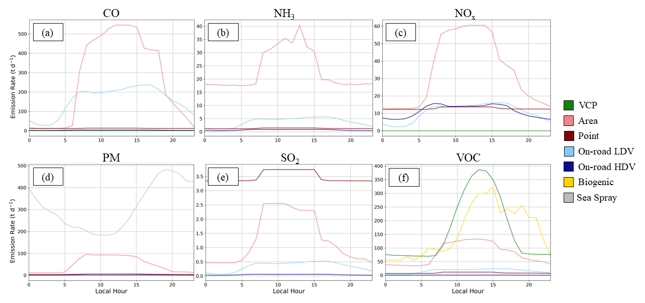
Figure 4Diurnal variations in the emission rates averaged over 1–30 April 2020 and summed over the LA domain (with all ocean-covered cells removed) from all emission sources for (a) CO, (b) NH3, (c) NOx, (d) PM, (e) SO2, and (f) VOC.
2.1.4 Initial and boundary conditions
A nested modeling setup was used to provide the boundary conditions for the Los Angeles Basin. The Los Angeles Basin is represented by the domain shown in Fig. 2c, has a resolution of 1 km × 1 km, and is the domain of interest for this project. The initial and boundary conditions for the LA domain were provided by a coarse-resolution CMAQ simulation performed over a larger domain (Fig. 2b). The outer domain covering southern and central California has a resolution of 4 km × 4 km, and its air quality was simulated using the WRF and CMAQ scenarios described in Sect. 2.1.1–2.1.2. The emissions for this domain match the emissions described in Jiang et al. (2021). Publicly available seasonal average hemispheric CMAQ output was used as initial and boundary conditions for the California domain (Foley et al., 2023). The CMAQ predictions from the coarse-resolution California domain were used as initial and boundary conditions for the inner, finer-resolution LA domain.
2.2 Observational data
Observational data throughout the modeling domain are provided by the U.S. Environmental Protection Agency (EPA)'s Air Quality System (AQS) monitoring system (US EPA, 2013). These sites include measurements of O3, CO, NO, NO2, NOy, SO2, PM2.5, PM10, temperature, relative humidity, wind speed, and wind direction (not all sites contain all species at all times), and their locations are shown in Fig. 2b–c. In addition, gas- and aerosol-phase measurements were collected concurrent to the modeling period in Pasadena at Caltech. The Caltech air quality system (CITAQS) measures O3, CO, NO, NO2, NOy, SO2, and PM2.5 (Parker et al., 2020).
Measurements of PM1 (fine PM with diameters less than 1 µm) and its components (organic, NH4, NO3, SO4, and Cl) were performed using an Aerodyne high-resolution time-of-flight aerosol mass spectrometer (HR-ToF-AMS). Briefly, the AMS measures submicron, non-refractory PM1 (NR-PM1) at a high time resolution. During the 2020 measurement campaign, the AMS isokinetically sampled air from a stainless-steel line downstream of a 2.5 µm cut diameter Teflon-coated cyclone mounted on the roof of the Do you mean “Ronald and Maxine Linde Laboratory for Global Environmental Science at Caltech. Approximately 6 m of stainless-steel tubing connected the cyclone to the inlet of the HR-ToF-AMS. Standard methods were used to correct the data for gas-phase interferences and composition-dependent collection efficiencies (Middlebrook et al., 2012). Daily detection limits for aerosol chemical classes were calculated as 3 times the standard deviation of 30 min blank measurements made with a high-efficiency particulate arrestance (HEPA) filter. Daily detection limits for OA ranged from ∼ 0.1 to 0.3 µg m−3. The ionization efficiency of nitrate and relative ionization efficiency of ammonium was calibrated weekly, using 350 nm ammonium nitrate particles size-selected with a differential mobility analyzer.
Positive matrix factorization (PMF) was applied to the OA mass spectral datasets to gain insight into OA sources. The PMF results presented here were taken from a larger analysis of data collected in 2020 (8 April–19 July 2020). A detailed description of PMF solution selection is provided in Schulze et al. (2022). A total of five factors, corresponding to less-oxidized oxygenated OA (LO-OOA), more-oxidized oxygenated OA (MO-OOA), hydrocarbon-like OA (HOA), cooking-influenced OA (CIOA), and an organic-nitrate influenced LO-OOA (LO-OOA-ON), were extracted from the OA dataset. Factors were identified using correlations with known tracers and comparisons of mass spectral and diurnal profiles to those extracted previously in Los Angeles (Hayes et al., 2013) and other urban areas (Hu et al., 2016; Xu et al., 2016). For comparisons with model predictions, we combine the HOA and CIOA factors as primary OA (POA), though we note that SOA formed from low-volatility species may appear spectrally similar to HOA (Lambe et al., 2012), as discussed in Schulze et al. (2022).
Multiple statistics are used to compare modeled data to observed data. These are mean bias (MB), normalized mean bias (NMB), root mean square error (RMSE), and r2 (the square of the Pearson correlation coefficient), as defined below. In these equations, M is modeled data, O is observed data, is the mean of the modeled data, is the mean of the observed data, and N is the number of data points.
3.1 Evaluation of CTM inputs
3.1.1 Meteorology
The WRF predictions are compared to the AQS observations and the model performs very well in predicting temperature. The NMB values of temperature, relative humidity, wind speed, and wind direction at all AQS sites are calculated in the LA domain (Fig. 5), and statistics are averaged using all site data in Table S1 in the Supplement. Temperature is predicted well, with very low bias (NMB =3.8 %) and low scatter (r2=0.97). Relative humidity is moderately well predicted, with low scatter (r2=0.81) but non-negligible bias (NMB %). Errors in relative humidity will affect the water content of aerosols and the resulting partitioning of aqueous aerosol and the concentrations of other inorganic aerosol components like ammonium, nitrate, and chloride.
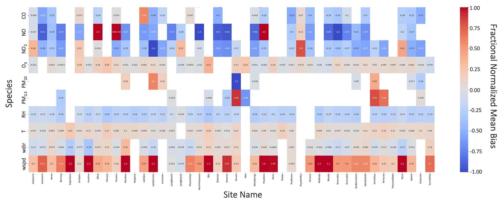
Figure 5Fractional NMB of pollutants (rows) at all EPA AQS sites (columns) in the LA domain, using daily average values from 1–30 April 2020. Empty boxes represent sites without measurements of the given pollutant.
Wind speed and direction tend not to be predicted well, with high bias and high scatter, but the error is highly variable between sites (Fig. 5). Wind speed and direction error will potentially affect the transport between grid cells, and their impact on modeled pollutant concentrations is investigated in Sect. 3.2. To understand the source of wind speed error, the NMB was quantified in all three modeling domains (Fig. S10). Wind speed did not improve appreciably as the model resolution increased, and the spatial distribution of error remained consistent. This suggests that the model error lies more with the input reanalysis data and less with the model configuration. This further suggests that to improve model simulations, new reanalysis data should be used or observational nudging should be engaged when running WRF. However, using new reanalysis data may introduce error to other meteorological fields, whereas temperature is well predicted by this model setup.
The domain-wide statistics (Table S1) capture data over a long time period and over sites with different meteorology, so the error at individual sites must be investigated when making site-specific comparisons. Despite the range of sites contained in these statistics, temperature is well predicted. This is critical, as temperature has a substantial impact on atmospheric chemistry and reaction rates.
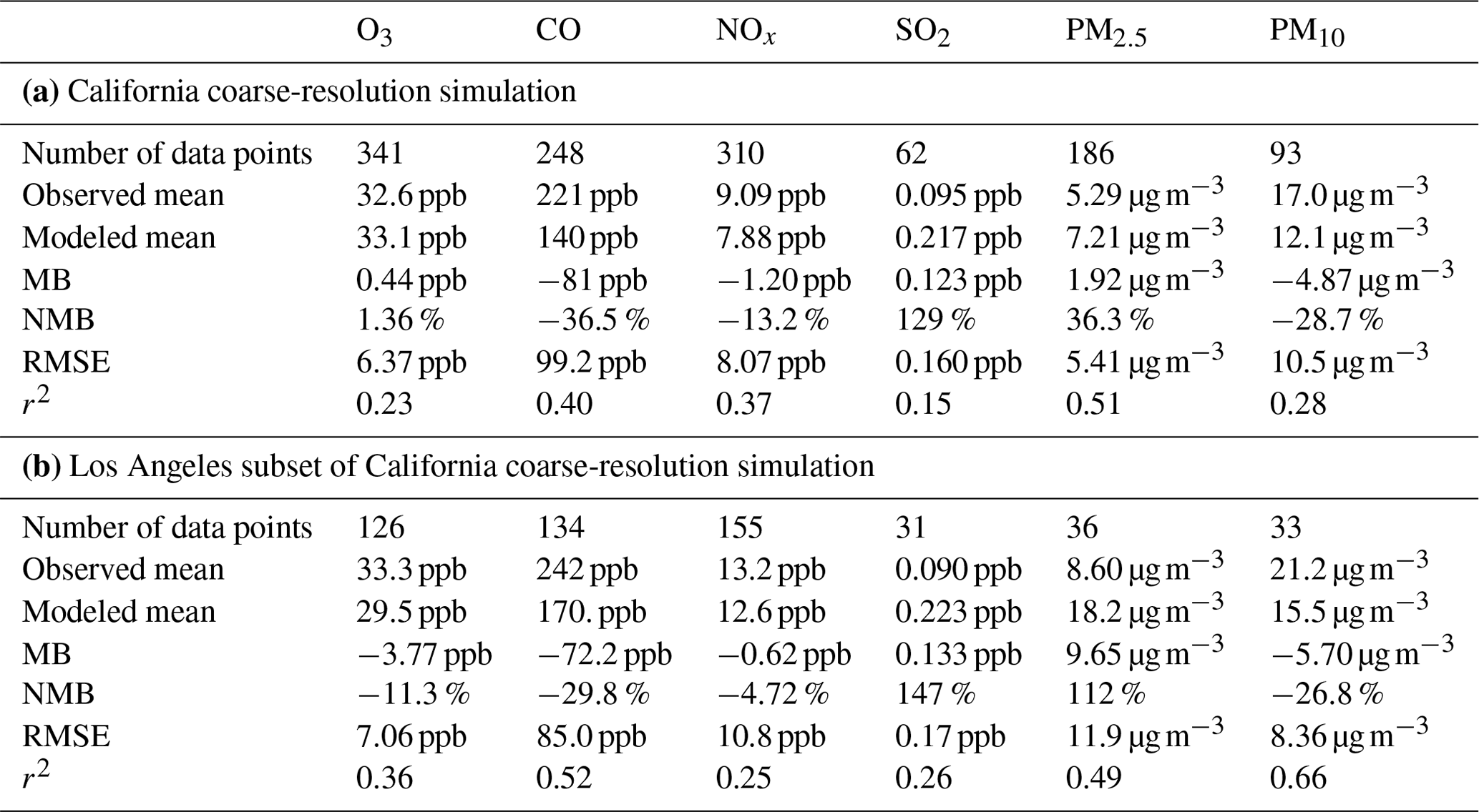
3.1.2 Coarse-resolution simulation results
California's coarse-resolution CMAQ simulation results provide the lateral chemical boundary conditions for the inner LA domain. Predicted pollutant concentrations from the coarse-resolution simulation of California are compared to EPA AQS monitoring site data in Table 1. O3 is well predicted, based on its low MB, NMB, and RMSE. CO, NOx, and PM10 are all underpredicted (MB and NMB), with moderately high scatter (RMSE and r2), while PM2.5 is overpredicted. SO2 is greatly overpredicted (MB and NMB). The accuracy of the region covering the Los Angeles Basin is of particular importance, since that region will provide the initial and boundary conditions for the fine-resolution domain. Those results are compared to AQS measurements (Table 1) and demonstrate some different behaviors when compared to the results of the full domain. NOx is slightly better predicted, while still underestimated, but O3 is now underpredicted and less accurate. The average PM2.5 mass increases substantially, as expected, due to the higher air pollution in LA compared to other regions in California. PM2.5 also becomes greatly overpredicted in the model (MB and NMB) and will be considered when evaluating the results of the fine-resolution simulation. The model bias remains approximately consistent for CO, SO2, and PM10.
Table 1Statistical analysis of daily averaged CMAQ predictions for the (a) coarse-resolution domain of California and the (b) LA Basin subset of the California domain, as compared to EPA AQS monitoring site data. Note that ppb stands for part per billion.
3.2 Evaluation of fine-resolution model predictions
Model predictions are compared to EPA AQS measurements at 44 sites in the domain (Figs. 5–6; Table S2). O3 has low NMB at all sites (NMB =10.2 %) despite high scatter (r2=0.30) and has the correct spatial distribution despite poorly predicted NOx. NO, NO2, and CO prediction errors can be positive or negative, depending on the location. PM measurements are limited in the domain and will be investigated further in Sect. 3.3–3.4. Domain-wide statistics are provided in Table S2. NOx and VOC concentrations are highest in polluted and high-emitting regions, and O3 titration by freshly emitted NO results in O3 concentrations that are lower in the urban core than in surrounding areas. Fine PM (PM1 and PM2.5) are highest in the urban center, while PM10 concentrations increase over the ocean due to sea spray aerosol. Because of the potential overprediction of sea spray emissions, it is possible that PM10 is overpredicted. POA is highest over high-emission regions, while SOA is highest over downwind regions, displaying the importance of chemical aging during transport.
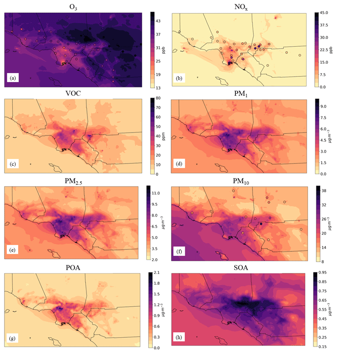
Figure 6Time-averaged (1–30 April 2020) CMAQ-predicted concentration of (a) O3 (parts per billion – ppb), (b) NOx (ppb), (c) total VOC (parts per million – ppm), (d) PM1 (µg m−3), (e) PM2.5 (µg m−3), (f) PM10 (µg m−3), (g) POA (µg m−3), and (h) SOA (µg m−3). Circles depict the average concentration measured at the EPA AQS site at that location. There are no AQS measurements of VOCs, PM1, POA, or SOA.
The impact of transport on modeled pollutant concentration was investigated by performing a sensitivity simulation with perturbed wind speed. The WRF wind speed was reduced by 25 % (i.e., scaled by a factor of 0.75) in an effort to correct for some of the wind speed bias (Fig. 5). A reduction of 25 % was chosen to represent the correction required to bring modeled wind speed into the range of observed wind speed, as represented by the values in Table S1. The results are presented below in Figs. 7 and 8 and can be compared to the base case wind speed bias in Fig. 5. Wind speed improved appreciably in response to the 25 % reduction in their values throughout the domain. In spite of improved wind speed, modeled O3 and PM2.5 did not improve. This suggests that wind speed does not have a large effect on modeled pollutant concentrations, and bias in those concentrations is more likely caused by errors in modeled chemistry and/or emissions.
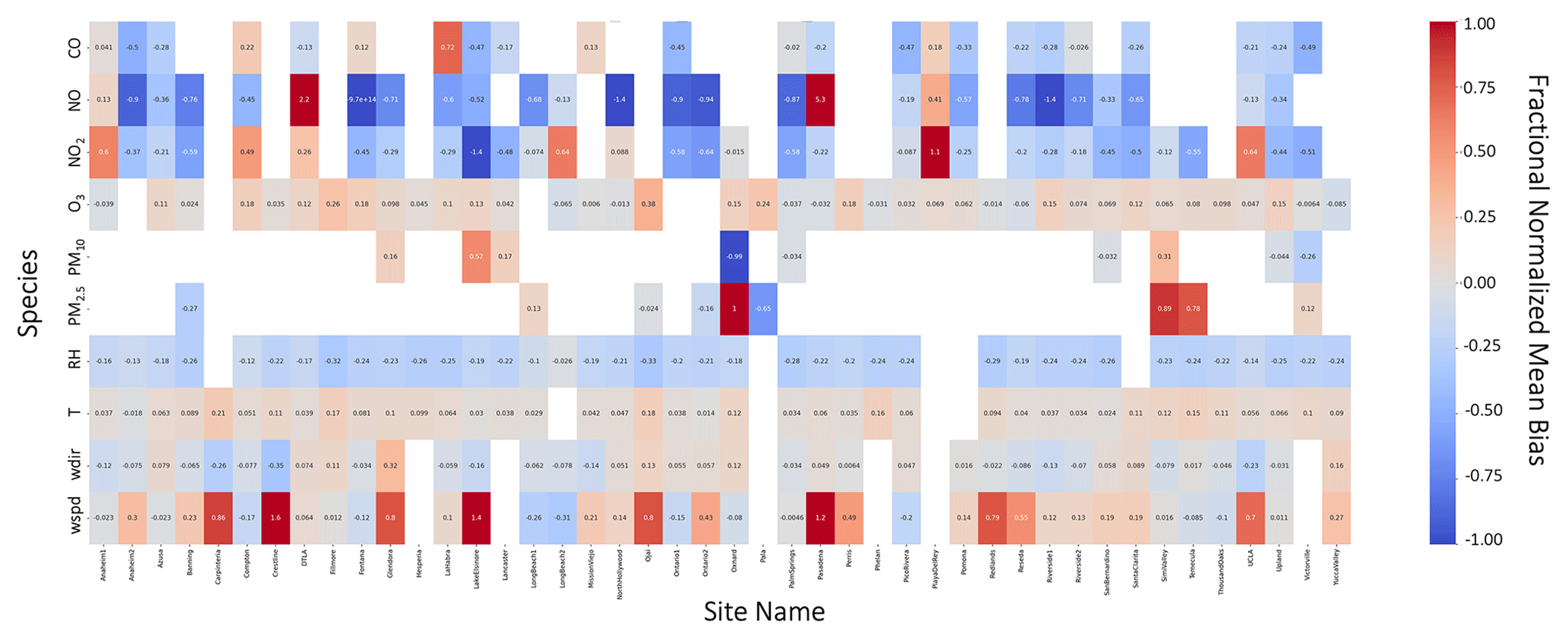
Figure 7Fractional NMB of pollutants (rows) at all EPA AQS sites (columns) in the LA domain using daily average values from 1–30 April 2020. Empty boxes represent sites without measurements of the given pollutant. Results presented here use default wind speed scaled by a factor of 0.75.
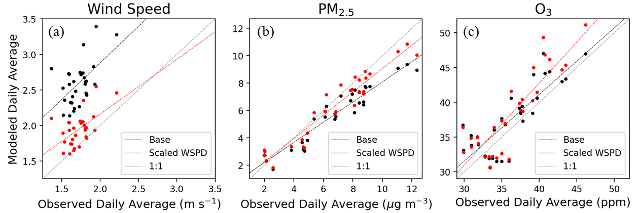
Figure 8Daily averaged modeled versus observed values of (a) wind speed, (b) PM2.5, and (c) O3. Black markers and lines represent data from the base case wind speed simulations. Red markers and lines represent data from the scaled (i.e., scaled by 0.75) wind speed simulations. The gray line represents the 1:1 modeled : observed line.
3.3 Evaluation of aerosol chemistry by ground-based observations in Pasadena
Modeled PM1 is underestimated due primarily to a large underestimation of OA. The PM1 mass and composition in Pasadena measured by AMS and predicted by CMAQ are compared in Fig. 9. All predicted inorganic component (SO4, NO3, NH4, and Cl) concentrations are smaller by mass than observed values. It is worth noting that PM1 NO3 is nearly well predicted (Table S3), despite gaseous NOx underpredictions (Table S4). The model additionally predicts “other” inorganic PM1, which includes elemental carbon (EC), soil, and crustal elements, which is not measured at the Pasadena ground site. The overall PM1 bias (NMB %) is caused by the large underprediction of OA (NMB %). POA is well predicted (Fig. 10a), and the diurnal trend matches predictions, except during the late night and early morning hours (Fig. 10b). SOA is significantly underpredicted (Fig. 10a) and has an accurate diurnal trend, except during early morning (Fig. 10b). During the day when emissions and photochemistry are at maximum, we measured and observed SOA peaks. SOA decreases in the evening as emissions decrease. Despite the lower photochemistry and emissions, SOA (and other pollutant levels) remain high at night due to low planetary boundary layer (PBL) height. The accurate representation of POA and poorer representation of SOA suggests that OA is better represented near source regions and diminishes in its effectiveness with distance from sources.
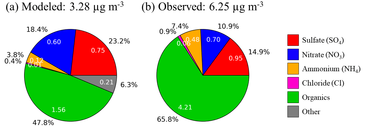
Figure 9PM1 composition averaged over 8–30 April 2020 in Pasadena, as (a) predicted by CMAQ and (b) measured by AMS. Values inside the pie represent average mass values (µg m−3), and values outside the pie represent the percentage of the total mass of each component.
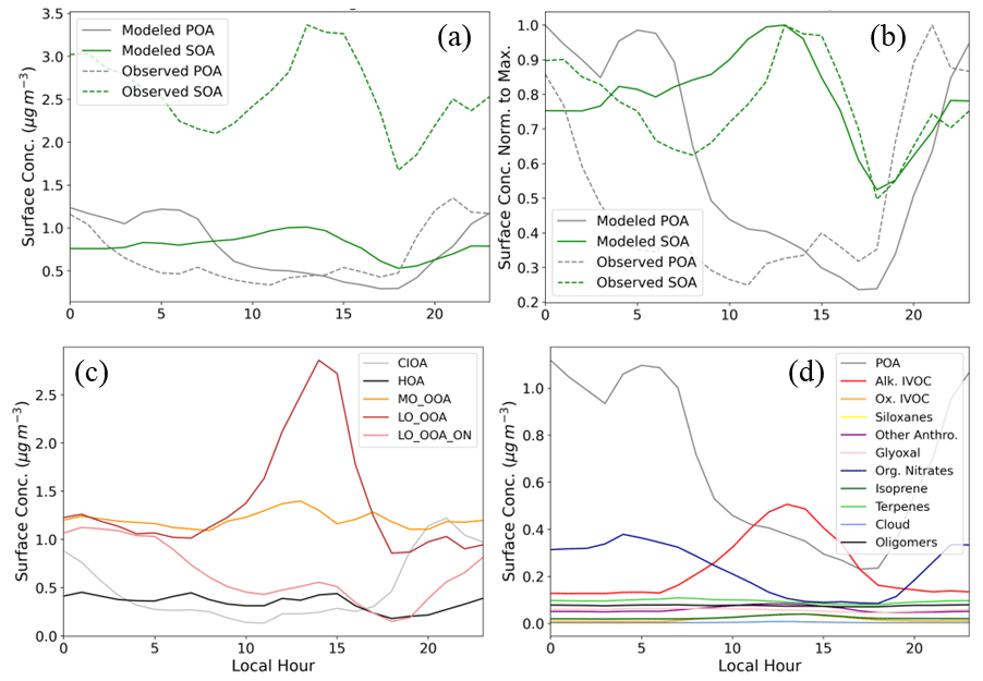
Figure 10(a) Modeled (solid) and measured (dashed) POA (gray) and SOA (green) diurnal variation in Pasadena. (b) Modeled (solid) and measured (dashed) POA (gray) and SOA (green) diurnal variation in Pasadena. Surface concentration was normalized to the daily maximum surface concentration. (c) PMF-calculated POA and SOA speciation in Pasadena. (d) Model-predicted POA and SOA speciation in Pasadena. All diurnal trends are calculated for 8–30 April 2020.
Detailed model speciation and source apportionment can be used to understand the major sources of OA precursors in Pasadena and the error in SOA predictions. Measured POA comprises cooking-influenced OA (CIOA) and hydrocarbon-like OA (HOA). CIOA peaks overnight, due to the PBL height dilution effect during the day, while HOA remains high throughout the day, due to high local primary emissions sources (Fig. 10). Measured SOA comprises more-oxidized oxygenated OA (MO-OOA), less-oxidized oxygenated OA (LO-OOA), and LO-OOA associated with organic nitrates (LO-OOA-ON). MO-OOA is consistently one of the largest OA components, with little diurnal variation. LO-OOA is the largest SOA component and has a sharp peak at midday, which is consistent with higher oxidation rates during midday. Modeled alkane-like IVOCs have a similar high peak around midday, although of a smaller magnitude (Fig. 10d). LO-OOA-ON have a small midday peak, suggesting some photochemical production, but the largest contribution from LO-OOA-ON is overnight. This could be due in part to the PBL effect and may also be due to overnight NO3 chemistry producing organic nitrates. This is consistent with the overnight peak of modeled organic nitrates (Fig. 10d) and terpene- and glyoxal-derived SOA (Fig. S11), which are biogenic in nature. All other modeled SOA species, except oligomers, have low overnight mass and peak at midday, but their magnitudes are small, which are likely a source of error in the CMAQ chemical mechanism. CMAQ lacks species which are behaving like LO-OOA, and the inclusion of additional SOA precursor species could improve SOA predictions (Pye et al., 2023). One potential source of error could be yields of species that are too low and that already exist in the model, such as aromatics, which have not been corrected for gas-phase wall losses (Zhang et al., 2014). Additional sources of error could include missing emissions, such as from asphalt, which would peak during midday when temperatures are highest, consistent with LO-OOA.
3.4 LA Basin source apportionment
The impact of removing each emission source on O3 is presented in Fig. 11, and these changes can be understood by investigating the changes in NOx, VOC, and OH (Figs. S13–S15). The impact of sea spray is small because sea spray emits only particles, so those results are presented in Fig. S12. O3 decreased everywhere in response to the removal of VCP and biogenic emissions. VCPs only emit VOCs, and so the elimination of VCP emissions leads to VOC decreases everywhere. In response, OH and NOx concentrations increase, and the importance of transport and secondary aging processes is evident by the downwind location of most of the OH increase. The O3 decrease resulting from VOC decreases is consistent with NOx-saturated behavior, which has typically described highly polluted urban areas. The removal of biogenic emissions has a similar response, as biogenic sources mainly emit VOCs. One exception lies in the fact that biogenic sources also emit NO, so the VOC : NOx ratio changes less and thus biogenics have a smaller impact on O3 change than VCPs do. In both cases of VCP and biogenic emissions removal, the outer regions display less sensitivity, as a reduction in VOCs results in a near-zero change in O3.
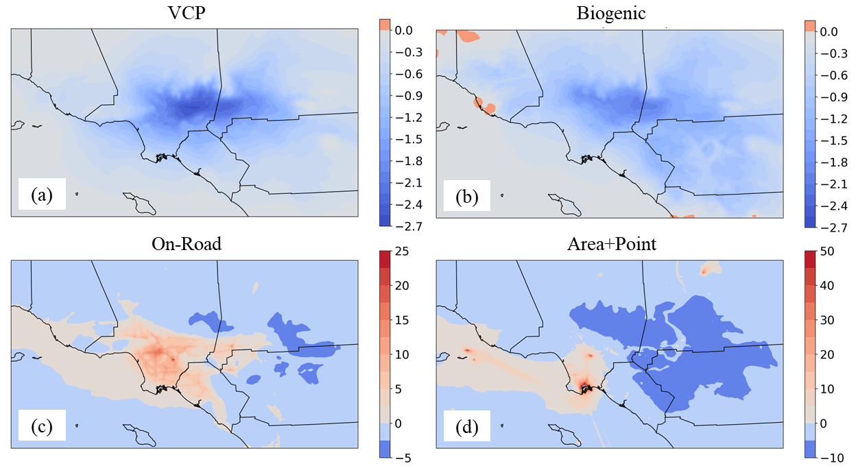
Figure 11Percent change in the average (1–30 April 2020) predicted O3 concentration averaged over 1–30 April 2020 and caused by removing each emission source. (a) VCP, (b) biogenic, (c) on-road vehicles, and (d) area+point.
On-road vehicles and area+point sources emit NOx, VOC, particles, and other inorganic gas-phase species. When these emission sources are removed, VOC and NOx concentrations decrease everywhere. In the urban core, where VOC and NOx concentrations are high, OH and O3 increase in response to the combined on-road VOC and NOx reductions. This is characteristic of the effect of large NOx relative to VOC (Fig. 4) reductions under NOx-saturated conditions. In contrast, the outer regions display behavior closer to NOx-limited behavior, where VOC and NOx reductions result in OH and O3 reductions. The reductions are small, suggesting that O3 is not sensitive to emission reductions in these regions. The elimination of area+point source emissions has a similar impact on O3. OH and O3 increase in the urban core, with a decrease in OH and O3 in the outer regions. The importance of ships and the Long Beach Port is evident, but it is likely that shipping emissions of NOx are overestimated relative to other area source emissions (Fig. S8), and so this impact may be overstated in these results.
PM2.5 concentrations decrease everywhere in response to emission reductions (Fig. 12). VCPs and biogenic sources emit only gas-phase species, so PM is formed exclusively via secondary processes. Biogenic PM is formed mostly over high-emission areas like mountains, while VCP-derived PM is found in downwind regions, highlighting the importance of secondary formation during transport, similar to O3 formation (Fig. 11). PM from on-road and area+point sources is predominantly emitted directly because most of the impact to PM2.5 is located in high-emission regions. This is in spite of the increased oxidation capacity in the high-emission regions (Fig. S13). So if the emissions are removed entirely, as in this study, PM2.5 will decrease. However, if the emissions were not entirely removed, the increased OH and the nonlinearity of atmospheric chemistry could lead to increased PM. Sea spray particles are reduced along the coastline where waves break (Fig. S16).
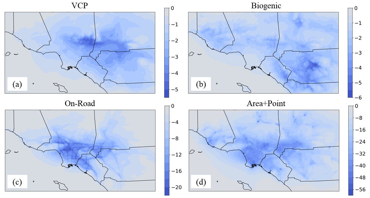
Figure 12Percent change in the average (1–30 April 2020) predicted PM2.5 concentration caused by removing each emission source. (a) VCP, (b) biogenic, (c) on-road vehicles, and (d) area+point.
Different species impact the PM2.5 change from each emission source (Fig. S17). On-road sources primarily decrease the NO3 and NH4 components of PM2.5, both by direct emission and emissions of gas-phase NOx. The reduction in the on-road VOCs has relatively little impact on the organic fraction of PM2.5. Area+point emissions also reduce PM2.5 NO3 and NH4, plus other direct emissions like POA and EC. VCPs and biogenic sources emit only VOCs, so they impact mostly the SOA fraction of PM2.5. The reduction in the VOCs leads to increases in OH and NOx and thus increases in the PM2.5 NO3 and NH4.
SOA decreases almost everywhere in response to the removal of emission sources but can increase in some high-emission regions (Fig. 13). The SOA change from VCPs is downwind of the main emission regions. Biogenic SOA decrease is located mostly in remote, mountainous regions. Downwind SOA decreases when all on-road emissions are removed, but SOA in the downtown LA region increases. This occurs because it is NOx-saturated and has increased OH concentrations (Fig. S13), which increases rates of VOC oxidation and therefore SOA formation. The SOA decrease from the removal of the area+point emission sources is more widely distributed than the emissions themselves (Fig. S2–S7), displaying the importance of SOA formation during transport.
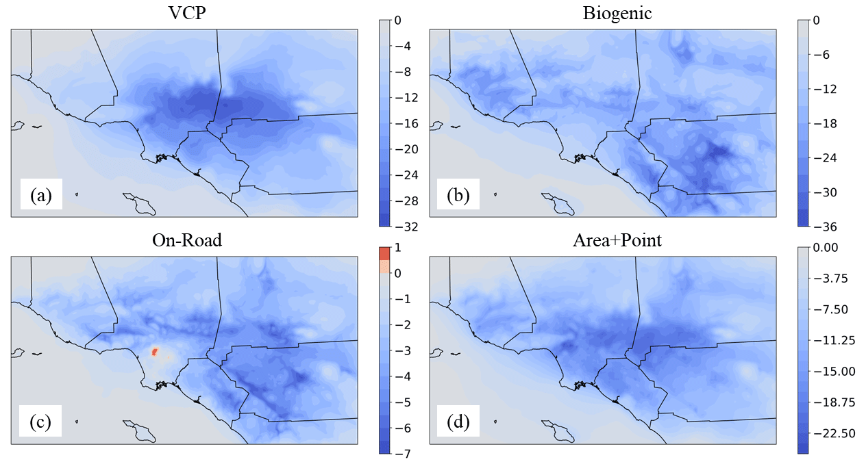
Figure 13Percent change in the average (1–30 April 2020) predicted SOA concentration caused by removing each emission source. (a) VCP, (b) biogenic, (c) on-road vehicles, and (d) area+point.
SOA speciation varies throughout the domain and is dependent on location-specific emissions and meteorology (Fig. S18). The largest components of SOA are derived from alkane-like IVOCs, organic nitrates, and monoterpenes. Alkane-like IVOC concentrations are highest downwind of high-emissions regions, demonstrating the importance of secondary formation during transport. Organic nitrate concentrations are highest over high-emission areas, where VOC and NOx concentrations are largest. Monoterpene concentrations are more uniform and have both anthropogenic (i.e., VCP) and biogenic sources. Little SOA throughout the domain is formed from siloxanes, sesquiterpenes, or cloud processing. Biogenic SOA is primarily derived from sesquiterpenes, monoterpenes, and isoprenes, and these aerosol species dominate over mountainous and remote areas in the outer regions of the domain.
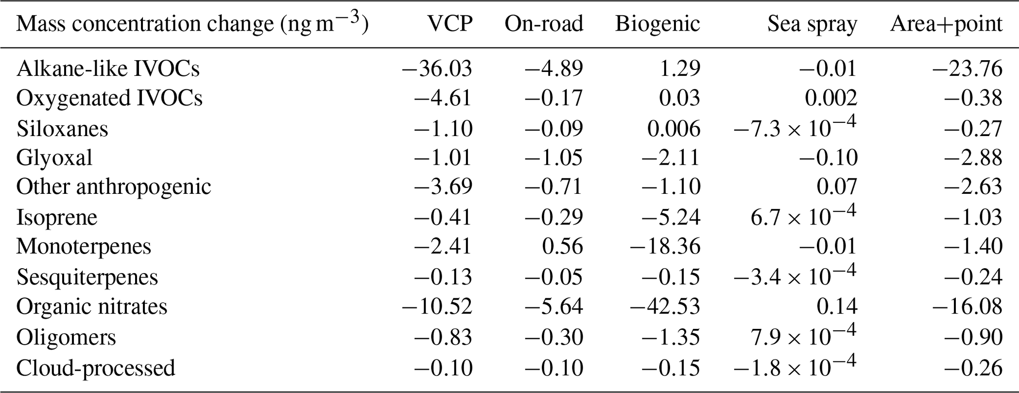
SOA formation chemistry can be further understood by investigating the source apportionment of SOA components in Pasadena. The impact of removing each emission source on each modeled SOA component is given in Table 2. The main component of SOA – alkane-like IVOCs – originates particularly from VCPs and area+point emission sources. Alkane-like IVOCs are emitted from VCPs as low-volatility gases, while they are evaporated and oxidized POA from area+point emission sources. Organic nitrates have important contributions from VCPs and area+point emission sources but are mostly formed from biogenic precursors. Despite VCP, biogenic, and area+point emission sources being highest during the daytime, organic nitrates peak overnight due to nighttime NO3 chemistry. In general, our modeling suggests SOA in LA is mostly driven by VCP, area, and point emission sources.
Table 2Mass concentration change (ng m−3) of SOA components averaged over the LA domain when each emission source is removed.
This study presents a new model framework to simulate air quality in Los Angeles. Past modeling studies of LA focus on 2010 to overlap with the California Research at the Nexus of Air Quality and Climate Change (CalNex) campaign, and few exist which focus on SOA sources and speciation. We developed state-of-the-science inputs of meteorology, emissions, and boundary conditions and show that these inputs are comparable to observations. Emissions are separated into three anthropogenic categories – VCP, on-road, and area+point – and two natural categories – gases and sea spray – allowing for source apportionment studies.
The model is set up for April 2020, and the results are compared to observations, aiming to better understand the chemistry leading to pollutant formation. Temperature and O3 are very well predicted, but NOx and PM are underpredicted. In particular, OA is underpredicted in Pasadena when compared to AMS measurements. While POA is well predicted, SOA is greatly underpredicted. The main components of modeled SOA are alkane-like IVOCs and organic nitrates, while other categories of SOA are likely underpredicted (for example, oxygenated IVOCs which have not been well classified in laboratory settings).
This study stresses that improved model predictions will require updated chemistry and emissions. The chemistry of SVOCs is not well understood, and better representations should be included in CMAQ as they are developed. SVOCs are also typically not represented in emission inventories, and while the VCP inventory used here utilizes new SVOC speciation profiles, the other categories of emissions did not specifically study SVOCs. The chemistry of oxygenated species has not been extensively studied and should be focused on in future work, due to the prevalence of oxygenated emissions and atmospheric constituents (Pennington et al., 2021). Some emissions from anthropogenic sources are likely underpredicted. For example, boats are estimated to emit more NOx than off-road sources, but off-road sources should likely be the main area source of NOx (Khare and Gentner, 2018). Also, many forms of asphalt emissions are not included in VCP or area sources but likely will contribute significant SOA and therefore reduce modeled SOA bias (Khare and Gentner, 2018).
The source apportionment results convey important qualities about the VOC–NOx regime of the LA atmosphere. The urban core of LA demonstrates NOx-saturated behavior; NOx reductions lead to O3 increase, while VOC reductions lead to O3 decrease. Outside of the urban core, O3 decreases in response to any level of either NOx or VOC removal, suggesting a regime that is less NOx-saturated than the urban region, such as a regime lying close to the O3–NOx–VOC ridgeline in the VOC-sensitive regime (Seinfeld and Pandis, 2016). Reducing O3 is a consistent goal for policymakers, and this work shows that O3 in Los Angeles is reduced by the removal of VOCs. NOx emission decreases remain important, as these decreases will move the LA Basin from a NOx-saturated regime closer to a NOx-sensitive regime. However, NOx reductions without concurrent or larger reductions in VOC concentrations will make O3 pollution worse until the NOx-sensitive regime is reached. VCPs emit the highest amount of VOCs from anthropogenic activities and thus may be particularly effective to target for a reduction in O3. It is also important to consider the spatial distribution of emissions and reduction policies. Reducing NOx and/or VOC emissions in the outer regions of the domain will have a lesser impact than reductions in the urban core or may have an opposite effect, as demonstrated in this study. The increased oxidative capacity of the NOx-saturated regions also has an impact on SOA formation and the formation of secondary inorganic components of PM. Focusing on emissions in the urban core is critical and will affect downwind regions. It should be noted that this study was performed in the spring season, which is not peak ozone season. Thus, results may differ in the summer months, and further studies should investigate this period.
In Part 2, the new model framework is used to investigate future emission scenarios involving VCP and on-road vehicle emissions during the 2020 lockdown of the pandemic. VCP emissions have been quantified in multiple studies (i.e., Seltzer et al., 2021; McDonald et al., 2018), but none of these studies has investigated the implications of future VCP emissions. We reduce VCP emissions to investigate the impact on O3, NOx, PM, and SOA speciation. Additionally, we run the model in a “non-COVID-19” scenario, where on-road emissions are represented without COVID-19-induced VMT reductions. In this way, the impact of emissions versus meteorology on 2020 air quality can be distinguished. Understanding these possible outcomes can shape informed policy decisions.
The following data used in this article have been deposited on Stanford Digital Repository (DOI: https://doi.org/10.25740/qc346hv0119, Wang et al., 2024)
-
CMAQ source code
-
WRF namelist files
-
CMAQ processing scripts.
The supplement related to this article is available online at: https://doi.org/10.5194/acp-24-2345-2024-supplement.
EAP, YW, and JHS designed and led the research project. EAP performed all model simulations and drafted the paper. EAP, YW, and JHS analyzed the data. BCS collected AMS data and performed PMF analysis. KMS provided VCP emissions. JY provided VMT data. ZJ and BZ provided emissions for the California 4 km × 4 km domain. MV provided the CARB emissions inventory and all SMOKE input files. DC provided the EMFAC emissions inventory. BNM and HOTP participated in useful research discussions and mentored EAP. CMK and RXW collected AMS data. All authors participated in useful research discussions and revised the paper.
At least one of the (co-)authors is a member of the editorial board of Atmospheric Chemistry and Physics. The peer-review process was guided by an independent editor, and the authors also have no other competing interests to declare.
The views expressed in this article are those of the authors and do not necessarily represent the views or policies of the U.S. Environmental Protection Agency.
Publisher’s note: Copernicus Publications remains neutral with regard to jurisdictional claims made in the text, published maps, institutional affiliations, or any other geographical representation in this paper. While Copernicus Publications makes every effort to include appropriate place names, the final responsibility lies with the authors.
The authors would like to thank Leonardo Ramirez, for his guidance on the CARB emission inventories, and Han Kim, for introducing and explaining useful Python analysis tools. We are also grateful to John Crounse and Harrison Parker for managing the CITAQS station and collecting the CITAQS data used in this study. Elyse A. Pennington and John H. Seinfeld acknowledge funding support from the Samsung Global Research Outreach Program. Yuan Wang and John H. Seinfeld acknowledge funding support from the National Science Foundation (grant no. AGS-2103714). We also acknowledge high-performance computing support from NASA Pleiades.
This research has been supported by the Samsung Global Research Outreach Program and the National Science Foundation (grant no. AGS-2103714).
This paper was edited by Manabu Shiraiwa and reviewed by two anonymous referees.
Alapaty, K., Niyogi, D., Chen, F., Pyle, P., Chandrasekar, A., and Seaman, N.: Development of the Flux-Adjusting Surface Data Assimilation System for Mesoscale Models, J. Appl. Meteorol. Clim., 47, 2331–2350, https://doi.org/10.1175/2008JAMC1831.1, 2008.
Appel, K. W., Bash, J. O., Fahey, K. M., Foley, K. M., Gilliam, R. C., Hogrefe, C., Hutzell, W. T., Kang, D., Mathur, R., Murphy, B. N., Napelenok, S. L., Nolte, C. G., Pleim, J. E., Pouliot, G. A., Pye, H. O. T., Ran, L., Roselle, S. J., Sarwar, G., Schwede, D. B., Sidi, F. I., Spero, T. L., and Wong, D. C.: The Community Multiscale Air Quality (CMAQ) model versions 5.3 and 5.3.1: system updates and evaluation, Geosci. Model Dev., 14, 2867–2897, https://doi.org/10.5194/gmd-14-2867-2021, 2021.
Bahreini, R., Middlebrook, A. M., de Gouw, J. A., Warneke, C., Trainer, M., Brock, C. A., Stark, H., Brown, S. S., Dube, W. P., Gilman, J. B., Hall, K., Holloway, J. S., Kuster, W. C., Perring, A. E., Prevot, A. S. H., Schwarz, J. P., Spackman, J. R., Szidat, S., Wagner, N. L., Weber, R. J., Zotter, P., and Parrish, D. D.: Gasoline emissions dominate over diesel in formation of secondary organic aerosol mass, Geophys. Res. Lett., 39, L06805, https://doi.org/10.1029/2011GL050718, 2012.
Bash, J. O., Baker, K. R., and Beaver, M. R.: Evaluation of improved land use and canopy representation in BEIS v3.61 with biogenic VOC measurements in California, Geosci. Model Dev., 9, 2191–2207, https://doi.org/10.5194/gmd-9-2191-2016, 2016.
California Air Resources Board: EMFAC2017 Volume III - Technical Documentation, V1.0.2, https://ww2.arb.ca.gov/sites/default/files/2023-01/emfac2017-volume-iii-technical-documentation.pdf (last access: 22 September 2023), 2018.
Caltrans: Caltrans PeMS, https://pems.dot.ca.gov/ (last access: 22 September 2023), 2020.
CARB: Criteria Pollutant Emission Inventory Data, California Air Resources Board, https://ww2.arb.ca.gov/criteria-pollutant-emission-inventory-data (last access: 15 September 2022), 2020.
Carlton, A. G., Bhave, P. V., Napelenok, S. L., Edney, E. O., Sarwar, G., Pinder, R. W., Pouliot, G. A., and Houyoux, M.: Model Representation of Secondary Organic Aerosol in CMAQv4.7, Environ. Sci. Technol., 44, 8553–8560, https://doi.org/10.1021/es100636q, 2010.
Carter, W. P. L.: Development of the SAPRC-07 chemical mechanism, Atmos. Environ., 44, 5324–5335, https://doi.org/10.1016/j.atmosenv.2010.01.026, 2010.
Choi, Y., Kim, J., Eldering, A., Osterman, G., Yung, Y. L., Gu, Y., and Liou, K. N.: Lightning and anthropogenic NOx sources over the United States and the western North Atlantic Ocean: Impact on OLR and radiative effects, Geophys. Res. Lett., 36, L17806, https://doi.org/10.1029/2009GL039381, 2009.
CMAS: SMOKE (Sparse Matrix Operator Kerner Emissions) Modeling System, CMAS: Community Modeling and Analysis System, https://www.cmascenter.org/smoke/index.cfm (last access: 22 September 2023), 2020.
Donahue, N. M., Epstein, S. A., Pandis, S. N., and Robinson, A. L.: A two-dimensional volatility basis set: 1. organic-aerosol mixing thermodynamics, Atmos. Chem. Phys., 11, 3303–3318, https://doi.org/10.5194/acp-11-3303-2011, 2011.
Ensberg, J. J., Hayes, P. L., Jimenez, J. L., Gilman, J. B., Kuster, W. C., de Gouw, J. A., Holloway, J. S., Gordon, T. D., Jathar, S., Robinson, A. L., and Seinfeld, J. H.: Emission factor ratios, SOA mass yields, and the impact of vehicular emissions on SOA formation, Atmos. Chem. Phys., 14, 2383–2397, https://doi.org/10.5194/acp-14-2383-2014, 2014.
Fahey, K. M., Carlton, A. G., Pye, H. O. T., Baek, J., Hutzell, W. T., Stanier, C. O., Baker, K. R., Appel, K. W., Jaoui, M., and Offenberg, J. H.: A framework for expanding aqueous chemistry in the Community Multiscale Air Quality (CMAQ) model version 5.1, Geosci. Model Dev., 10, 1587–1605, https://doi.org/10.5194/gmd-10-1587-2017, 2017.
Foley, K. M., Pouliot, G. A., Eyth, A., Aldridge, M. F., Allen, C., Appel, K. W., Bash, J. O., Beardsley, M., Beidler, J., Choi, D., Farkas, C., Gilliam, R. C., Godfrey, J., Henderson, B. H., Hogrefe, C., Koplitz, S. N., Mason, R., Mathur, R., Misenis, C., Possiel, N., Pye, H. O. T., Reynolds, L., Roark, M., Roberts, S., Schwede, D. B., Seltzer, K. M., Sonntag, D., Talgo, K., Toro, C., Vukovich, J., Xing, J., and Adams, E.: 2002–2017 Anthropogenic Emissions Data for Air Quality Modeling over the United States, Data in Brief, 47, 109022, https://doi.org/10.1016/j.dib.2023.109022, 2023.
Fountoukis, C. and Nenes, A.: ISORROPIA II: a computationally efficient thermodynamic equilibrium model for aerosols, Atmos. Chem. Phys., 7, 4639–4659, https://doi.org/10.5194/acp-7-4639-2007, 2007.
Gantt, B., Kelly, J. T., and Bash, J. O.: Updating sea spray aerosol emissions in the Community Multiscale Air Quality (CMAQ) model version 5.0.2, Geosci. Model Dev., 8, 3733–3746, https://doi.org/10.5194/gmd-8-3733-2015, 2015.
Gentner, D. R., Jathar, S. H., Gordon, T. D., Bahreini, R., Day, D. A., El Haddad, I., Hayes, P. L., Pieber, S. M., Platt, S. M., de Gouw, J., Goldstein, A. H., Harley, R. A., Jimenez, J. L., Prévôt, A. S. H., and Robinson, A. L.: Review of Urban Secondary Organic Aerosol Formation from Gasoline and Diesel Motor Vehicle Emissions, Environ. Sci. Technol., 51, 1074–1093, https://doi.org/10.1021/acs.est.6b04509, 2017.
Goliff, W. S., Stockwell, W. R., and Lawson, C. V.: The regional atmospheric chemistry mechanism, version 2, Atmos. Environ., 68, 174–185, https://doi.org/10.1016/j.atmosenv.2012.11.038, 2013.
Hayes, P. L., Ortega, A. M., Cubison, M. J., Froyd, K. D., Zhao, Y., Cliff, S. S., Hu, W. W., Toohey, D. W., Flynn, J. H., Lefer, B. L., Grossberg, N., Alvarez, S., Rappenglück, B., Taylor, J. W., Allan, J. D., Holloway, J. S., Gilman, J. B., Kuster, W. C., de Gouw, J. A., Massoli, P., Zhang, X., Liu, J., Weber, R. J., Corrigan, A. L., Russell, L. M., Isaacman, G., Worton, D. R., Kreisberg, N. M., Goldstein, A. H., Thalman, R., Waxman, E. M., Volkamer, R., Lin, Y. H., Surratt, J. D., Kleindienst, T. E., Offenberg, J. H., Dusanter, S., Griffith, S., Stevens, P. S., Brioude, J., Angevine, W. M., Jimenez, J. L.: Organic aerosol composition and sources in Pasadena, California, during the 2010 CalNex campaign, J. Geophys. Res.-Atmos., 118, 9233–9257, https://doi.org/10.1002/jgrd.50530, 2013.
Hersbach, H., Bell, B., Berrisford, P., Biavati, G., Horányi, A., Muñoz Sabater, J., Nicolas, J., Peubey, C., Radu, R., Rozum, I., Schepers, D., Simmons, A., Soci, C., Dee, D., and Thépaut, J.-N.: ERA5 hourly data on pressure levels from 1979 to present, Copernicus Climate Change Service (C3S) Climate Data Store (CDS) [data set], https://doi.org/10.24381/cds.bd0915c6, 2018.
Hu, W., Hu, M., Hu, W., Jimenez, J. L., Yuan, B., Chen, W., Wang, M., Wu, Y., Chen, C., Wang, Z., Peng, J., Zeng, L., and Shao, M.: Chemical composition, sources, and aging process of submicron aerosols in Beijing: Contrast between summer and winter, J. Geophys. Res.-Atmos., 121, 1955–1977, https://doi.org/10.1002/2015JD024020, 2016.
Hyslop, N. P.: Impaired visibility: The air pollution people see, Atmos. Environ., 43, 182–195, https://doi.org/10.1016/j.atmosenv.2008.09.067, 2009.
Intergovernmental Panel on Climate Change (Ed.): Anthropogenic and Natural Radiative Forcing, in: Climate Change 2013 – The Physical Science Basis: Working Group I Contribution to the Fifth Assessment Report of the Intergovernmental Panel on Climate Change, Cambridge University Press, 659–740, https://doi.org/10.1017/CBO9781107415324.018, 2014.
Jiang, Z., Shi, H., Zhao, B., Gu, Y., Zhu, Y., Miyazaki, K., Lu, X., Zhang, Y., Bowman, K. W., Sekiya, T., and Liou, K.-N.: Modeling the impact of COVID-19 on air quality in southern California: implications for future control policies, Atmos. Chem. Phys., 21, 8693–8708, https://doi.org/10.5194/acp-21-8693-2021, 2021.
Jimenez, J. L., Canagaratna, M. R., Donahue, N. M., Prevot, A. S. H., Zhang, Q., Kroll, J. H., DeCarlo, P. F., Allan, J. D., Coe, H., Ng, N. L., Aiken, A. C., Docherty, K. S., Ulbrich, I. M., Grieshop, A. P., Robinson, A. L., Duplissy, J., Smith, J. D., Wilson, K. R., Lanz, V. A., Hueglin, C., Sun, Y. L., Tian, J., Laaksonen, A., Raatikainen, T., Rautiainen, J., Vaattovaara, P., Ehn, M., Kulmala, M., Tomlinson, J. M., Collins, D. R., Cubison, M. J., E., Dunlea, J., Huffman, J. A., Onasch, T. B., Alfarra, M. R., Williams, P. I., Bower, K., Kondo, Y., Schneider, J., Drewnick, F., Borrmann, S., Weimer, S., Demerjian, K., Salcedo, D., Cottrell, L., Griffin, R., Takami, A., Miyoshi, T., Hatakeyama, S., Shimono, A., Sun, J. Y., Zhang, Y. M., Dzepina, K., Kimmel, J. R., Sueper, D., Jayne, J. T., Herndon, S. C., Trimborn, A. M., Williams, L. R., Wood, E. C., Middlebrook, A. M., Kolb, C. E., Baltensperger, U., and Worsnop, D. R.: Evolution of Organic Aerosols in the Atmosphere, Science, 326, 1525–1529, https://doi.org/10.1126/science.1180353, 2009.
Keller, C. A. and Evans, M. J.: Application of random forest regression to the calculation of gas-phase chemistry within the GEOS-Chem chemistry model v10, Geosci. Model Dev., 12, 1209–1225, https://doi.org/10.5194/gmd-12-1209-2019, 2019.
Khare, P. and Gentner, D. R.: Considering the future of anthropogenic gas-phase organic compound emissions and the increasing influence of non-combustion sources on urban air quality, Atmos. Chem. Phys., 18, 5391–5413, https://doi.org/10.5194/acp-18-5391-2018, 2018.
Khare, P., Machesky, J., Soto, R., He, M., Presto, A. A., and Gentner, D. R.: Asphalt-related emissions are a major missing nontraditional source of secondary organic aerosol precursors, Science Advances, 6, eabb9785, https://doi.org/10.1126/sciadv.abb9785, 2020.
Lambe, A. T., Onasch, T. B., Croasdale, D. R., Wright, J. P., Martin, A. T., Franklin, J. P., Massoli, P., Kroll, J. H., Canagaratna, M. R., Brune, W. H., Worsnop, D. R., and Davidovits, P.: Transitions from Functionalization to Fragmentation Reactions of Laboratory Secondary Organic Aerosol (SOA) Generated from the OH Oxidation of Alkane Precursors, Environ. Sci. Technol., 46, 5430–5437, https://doi.org/10.1021/es300274t, 2012.
Le, T., Wang, Y., Liu, L., Yang, J., Yung, Y. L., Li, G., and Seinfeld, J. H.: Unexpected air pollution with marked emission reductions during the COVID-19 outbreak in China, Science, 369, 702–706, https://doi.org/10.1126/science.abb7431, 2020.
Lim, S. S., Vos, T., Flaxman, A. D., Danaei, G., Shibuya, K., Adair-Rohani, H., AlMazroa, M. A., Amann, M., Anderson, H. R., Andrews, K. G., Aryee, M., Atkinson, C., Bacchus, L. J., Bahalim, A. N., Balakrishnan, K., Balmes, J., Barker-Collo, S., Baxter, A., Bell, M. L., Blore, J. D., Blyth, F., Bonner, C., Borges, G., Bourne, R., Boussinesq, M., Brauer, M., Brooks, P., Bruce, N. G., Brunekreef, B., Bryan-Hancock, C., Bucello, C., Buchbinder, R., Bull, F., Burnett, R. T., Byers, T. E., Calabria, B., Carapetis, J., Carnahan, E., Chafe, Z., Charlson, F., Chen, H., Chen, J. S., Cheng, A. T.-A., Child, J. C., Cohen, A., Colson, K. E., Cowie, B. C., Darby, S., Darling, S., Davis, A., Degenhardt, L., Dentener, F., Des Jarlais, D. C., Devries, K., Dherani, M., Ding, E. L., Dorsey, E. R., Driscoll, T., Edmond, K., Ali, S. E., Engell, R. E., Erwin, P. J., Fahimi, S., Falder, G., Farzadfar, F., Ferrari, A., Finucane, M. M., Flaxman, S., Fowkes, F. G. R., Freedman, G., Freeman, M. K., Gakidou, E., Ghosh, S., Giovannucci, E., Gmel, G., Graham, K., Grainger, R., Grant, B., Gunnell, D., Gutierrez, H. R., Hall, W., Hoek, H. W., Hogan, A., Hosgood, H. D., Hoy, D., Hu, H., Hubbell, B. J., Hutchings, S. J., Ibeanusi, S. E., Jacklyn, G. L., Jasrasaria, R., Jonas, J. B., Kan, H., Kanis, J. A., Kassebaum, N., Kawakami, N., Khang, Y.-H., Khatibzadeh, S., Khoo, J.-P., Kok, C., Laden, F., Lalloo, R., Lan, Q., Lathlean, T., Leasher, J. L., Leigh, J., Li, Y., Lin, J. K., Lipshultz, S. E., London, S., Lozano, R., Lu, Y., Mak, J., Malekzadeh, R., Mallinger, L., Marcenes, W., March, L., Marks, R., Martin, R., McGale, P., McGrath, J., Mehta, S., Memish, Z. A., Mensah, G. A., Merriman, T. R., Micha, R., Michaud, C., Mishra, V., Hanafiah, K. M., Mokdad, A. A., Morawska, L., Mozaffarian, D., Murphy, T., Naghavi, M., Neal, B., Nelson, P. K., Nolla, J. M., Norman, R., Olives, C., Omer, S. B., Orchard, J., Osborne, R., Ostro, B., Page, A., Pandey, K. D., Parry, C. D., Passmore, E., Patra, J., Pearce, N., Pelizzari, P. M., Petzold, M., Phillips, M. R., Pope, D., Pope, C. A., Powles, J., Rao, M., Razavi, H., Rehfuess, E. A., Rehm, J. T., Ritz, B., Rivara, F. P., Roberts, T., Robinson, C., Rodriguez-Portales, J. A., Romieu, I., Room, R., Rosenfeld, L. C., Roy, A., Rushton, L., Salomon, J. A., Sampson, U., Sanchez-Riera, L., Sanman, E., Sapkota, A., Seedat, S., Shi, P., Shield, K., Shivakoti, R., Singh, G. M., Sleet, D. A., Smith, E., Smith, K. R., Stapelberg, N. J., Steenland, K., Stöckl, H., Stovner, L. J., Straif, K., Straney, L., Thurston, G. D., Tran, J. H., Van Dingenen, R., van Donkelaar, A., Veerman, J. L., Vijayakumar, L., Weintraub, R., Weissman, M. M., White, R. A., Whiteford, H., Wiersma, S. T., Wilkinson, J. D., Williams, H. C., Williams, W., Wilson, N., Woolf, A. D., Yip, P., Zielinski, J. M., Lopez, A. D., Murray, C. J., and Ezzati, M.: A comparative risk assessment of burden of disease and injury attributable to 67 risk factors and risk factor clusters in 21 regions, 1990–2010: A systematic analysis for the Global Burden of Disease Study 2010, The Lancet, 380, 2224–2260, https://doi.org/10.1016/S0140-6736(12)61766-8, 2012.
Lu, Q., Murphy, B. N., Qin, M., Adams, P. J., Zhao, Y., Pye, H. O. T., Efstathiou, C., Allen, C., and Robinson, A. L.: Simulation of organic aerosol formation during the CalNex study: updated mobile emissions and secondary organic aerosol parameterization for intermediate-volatility organic compounds, Atmos. Chem. Phys., 20, 4313–4332, https://doi.org/10.5194/acp-20-4313-2020, 2020.
McDonald, B. C., Gouw, J. A. de, Gilman, J. B., Jathar, S. H., Akherati, A., Cappa, C. D., Jimenez, J. L., Lee-Taylor, J., Hayes, P. L., McKeen, S. A., Cui, Y. Y., Kim, S.-W., Gentner, D. R., Isaacman-VanWertz, G., Goldstein, A. H., Harley, R. A., Frost, G. J., Roberts, J. M., Ryerson, T. B., and Trainer, M.: Volatile chemical products emerging as largest petrochemical source of urban organic emissions, Science, 359, 760–764, https://doi.org/10.1126/science.aaq0524, 2018.
Middlebrook, A. M., Bahreini, R., Jimenez, J. L., and Canagaratna, M. R.: Evaluation of Composition-Dependent Collection Efficiencies for the Aerodyne Aerosol Mass Spectrometer using Field Data, Aerosol Sci. Tech., 46, 258–271, https://doi.org/10.1080/02786826.2011.620041, 2012.
Murphy, B. N., Woody, M. C., Jimenez, J. L., Carlton, A. M. G., Hayes, P. L., Liu, S., Ng, N. L., Russell, L. M., Setyan, A., Xu, L., Young, J., Zaveri, R. A., Zhang, Q., and Pye, H. O. T.: Semivolatile POA and parameterized total combustion SOA in CMAQv5.2: impacts on source strength and partitioning, Atmos. Chem. Phys., 17, 11107–11133, https://doi.org/10.5194/acp-17-11107-2017, 2017.
Murphy, B. N., Nolte, C. G., Sidi, F., Bash, J. O., Appel, K. W., Jang, C., Kang, D., Kelly, J., Mathur, R., Napelenok, S., Pouliot, G., and Pye, H. O. T.: The Detailed Emissions Scaling, Isolation, and Diagnostic (DESID) module in the Community Multiscale Air Quality (CMAQ) modeling system version 5.3.2, Geosci. Model Dev., 14, 3407–3420, https://doi.org/10.5194/gmd-14-3407-2021, 2021.
Nuvolone, D., Petri, D., and Voller, F.: The effects of ozone on human health, Environ. Sci. Pollut. R., 25, 8074–8088, https://doi.org/10.1007/s11356-017-9239-3, 2018.
Odum, J. R., Hoffmann, T., Bowman, F., Collins, D., Flagan, R. C., and Seinfeld, J. H.: Gas/Particle Partitioning and Secondary Organic Aerosol Yields, Environ. Sci. Technol., 30, 2580–2585, https://doi.org/10.1021/es950943+, 1996.
Parker, H. A., Hasheminassab, S., Crounse, J. D., Roehl, C. M., and Wennberg, P. O.: Impacts of Traffic Reductions Associated With COVID-19 on Southern California Air Quality, Geophys. Res. Lett., 47, e2020GL090164, https://doi.org/10.1029/2020GL090164, 2020.
Pennington, E. A., Seltzer, K. M., Murphy, B. N., Qin, M., Seinfeld, J. H., and Pye, H. O. T.: Modeling secondary organic aerosol formation from volatile chemical products, Atmos. Chem. Phys., 21, 18247–18261, https://doi.org/10.5194/acp-21-18247-2021, 2021.
Pleim, J. and Ran, L.: Surface Flux Modeling for Air Quality Applications, Atmosphere, 2, 3, https://doi.org/10.3390/atmos2030271, 2011.
Pye, H. O. T., Pinder, R. W., Piletic, I. R., Xie, Y., Capps, S. L., Lin, Y.-H., Surratt, J. D., Zhang, Z., Gold, A., Luecken, D. J., Hutzell, W. T., Jaoui, M., Offenberg, J. H., Kleindienst, T. E., Lewandowski, M., and Edney, E. O.: Epoxide Pathways Improve Model Predictions of Isoprene Markers and Reveal Key Role of Acidity in Aerosol Formation, Environ. Sci. Technol., 47, 11056–11064, https://doi.org/10.1021/es402106h, 2013.
Pye, H. O. T., Murphy, B. N., Xu, L., Ng, N. L., Carlton, A. G., Guo, H., Weber, R., Vasilakos, P., Appel, K. W., Budisulistiorini, S. H., Surratt, J. D., Nenes, A., Hu, W., Jimenez, J. L., Isaacman-VanWertz, G., Misztal, P. K., and Goldstein, A. H.: On the implications of aerosol liquid water and phase separation for organic aerosol mass, Atmos. Chem. Phys., 17, 343–369, https://doi.org/10.5194/acp-17-343-2017, 2017.
Pye, H. O. T., Place, B. K., Murphy, B. N., Seltzer, K. M., D'Ambro, E. L., Allen, C., Piletic, I. R., Farrell, S., Schwantes, R. H., Coggon, M. M., Saunders, E., Xu, L., Sarwar, G., Hutzell, W. T., Foley, K. M., Pouliot, G., Bash, J., and Stockwell, W. R.: Linking gas, particulate, and toxic endpoints to air emissions in the Community Regional Atmospheric Chemistry Multiphase Mechanism (CRACMM), Atmos. Chem. Phys., 23, 5043–5099, https://doi.org/10.5194/acp-23-5043-2023, 2023.
Qin, M., Murphy, B. N., Isaacs, K. K., McDonald, B. C., Lu, Q., McKeen, S. A., Koval, L., Robinson, A. L., Efstathiou, C., Allen, C., and Pye, H. O. T.: Criteria pollutant impacts of volatile chemical products informed by near-field modelling, Nature Sustainability, 4, 2, https://doi.org/10.1038/s41893-020-00614-1, 2021.
Ritchie, S. and Tok, Y. C.: Development of a New Methodology to Characterize Truck Body Types Along California Freeways California Air Resources Board, 11–316, p. 176, https://ww2.arb.ca.gov/sites/default/files/classic/research/apr/past/11-316.pdf (last access: 15 September 2022), 2016.
Robinson, A. L., Donahue, N. M., Shrivastava, M. K., Weitkamp, E. A., Sage, A. M., Grieshop, A. P., Lane, T. E., Pierce, J. R., and Pandis, S. N.: Rethinking Organic Aerosols: Semivolatile Emissions and Photochemical Aging, Science, 315, 1259–1262, https://doi.org/10.1126/science.1133061, 2007.
Sandermann Jr., H.: Ozone and Plant Health, Annu. Rev. Phytopathol., 34, 347–366, https://doi.org/10.1146/annurev.phyto.34.1.347, 1996.
Seinfeld, J. H. and Pandis, S. N.: Atmospheric Chemistry and Physics: From Air Pollution to Climate Change, 3rd edn., John Wiley & Sons, Inc., ISBN: 978-1118947401, 2016.
Seltzer, K. M., Pennington, E., Rao, V., Murphy, B. N., Strum, M., Isaacs, K. K., and Pye, H. O. T.: Reactive organic carbon emissions from volatile chemical products, Atmos. Chem. Phys., 21, 5079–5100, https://doi.org/10.5194/acp-21-5079-2021, 2021.
Seltzer, K. M., Murphy, B. N., Pennington, E. A., Allen, C., Talgo, K., and Pye, H. O. T.: Volatile Chemical Product Enhancements to Criteria Pollutants in the United States, Environ. Sci. Technol., https://doi.org/10.1021/acs.est.1c04298, 2022.
Skamarock, W. C., Klemp, J. B., Dudhia, J., Gill, D. O., and Barker, D.: A Description of the Advanced Research WRF Version 3, NCAR/TN-475+STR, University Corporation for Atmospheric Research, https://doi.org/10.5065/D68S4MVH, 2008.
US EPA: Air Quality System (AQS), US EPA, https://www.epa.gov/aqs (last access: 15 September 2022), 2013.
US EPA Office of Research and Development: CMAQ, Version 5.3.2, Zenodo [code], https://doi.org/10.5281/zenodo.4081737, 2020.
Wang, Y., Pennington, E., and Seinfeld, J.: CMAQ Model and scripts with Penning et al., 2024, ACP, Stanford Digital Repository [data set], https://doi.org/10.25740/qc346hv0119, 2024.
Xie, Y., Paulot, F., Carter, W. P. L., Nolte, C. G., Luecken, D. J., Hutzell, W. T., Wennberg, P. O., Cohen, R. C., and Pinder, R. W.: Understanding the impact of recent advances in isoprene photooxidation on simulations of regional air quality, Atmos. Chem. Phys., 13, 8439–8455, https://doi.org/10.5194/acp-13-8439-2013, 2013.
Xu, J., Shi, J., Zhang, Q., Ge, X., Canonaco, F., Prévôt, A. S. H., Vonwiller, M., Szidat, S., Ge, J., Ma, J., An, Y., Kang, S., and Qin, D.: Wintertime organic and inorganic aerosols in Lanzhou, China: sources, processes, and comparison with the results during summer, Atmos. Chem. Phys., 16, 14937–14957, https://doi.org/10.5194/acp-16-14937-2016, 2016.
Xu, L., Pye, H. O. T., He, J., Chen, Y., Murphy, B. N., and Ng, N. L.: Experimental and model estimates of the contributions from biogenic monoterpenes and sesquiterpenes to secondary organic aerosol in the southeastern United States, Atmos. Chem. Phys., 18, 12613–12637, https://doi.org/10.5194/acp-18-12613-2018, 2018.
Yang, J., Wen, Y., Wang, Y., Zhang, S., Pinto, J. P., Pennington, E. A., Wang, Z., Wu, Y., Sander, S. P., Jiang, J. H., Hao, J., Yung, Y. L., and Seinfeld, J. H.: From COVID-19 to future electrification: Assessing traffic impacts on air quality by a machine-learning model, P. Natl. Acad. Sci. USA, 118, e2102705118, https://doi.org/10.1073/pnas.2102705118, 2021.
Yarwood, G., Jung, J., Whitten, G. Z., Heo, G., Mellberg, J., and Estes, M.: Updates to the Carbon Bond Mechanism for Version 6 (CB6), 9th Annual CMAS Conference, Chapel Hill, NC, 11–13 October 2010.
Zhang, Q., Jimenez, J. L., Canagaratna, M. R., Allan, J. D., Coe, H., Ulbrich, I., Alfarra, M. R., Takami, A., Middlebrook, A. M., Sun, Y. L., Dzepina, K., Dunlea, E., Docherty, K., DeCarlo, P. F., Salcedo, D., Onasch, T., Jayne, J. T., Miyoshi, T., Shimono, A., Hatakeyama, S., Takegawa, N., Kondo, Y., Schneider, J., Drewnick, F., Borrmann, S., Weimer, S., Demerjian, K., Williams, P., Bower, K., Bahreini, R., Cottrell, L., Griffin, R. J., Rautiainen, J., Sun, J. Y., Zhang, Y. M., and Worsnop, D. R.: Ubiquity and dominance of oxygenated species in organic aerosols in anthropogenically-influenced Northern Hemisphere midlatitudes, Geophys. Res. Lett., 34, L13801, https://doi.org/10.1029/2007GL029979, 2007.
Zhang, X., Cappa, C. D., Jathar, S. H., McVay, R. C., Ensberg, J. J., Kleeman, M. J., and Seinfeld, J. H.: Influence of vapor wall loss in laboratory chambers on yields of secondary organic aerosol, P. Natl. Acad. Sci. USA, 111, 5802–5807, https://doi.org/10.1073/pnas.1404727111, 2014.
Zhao, Y., Nguyen, N. T., Presto, A. A., Hennigan, C. J., May, A. A., and Robinson, A. L.: Intermediate Volatility Organic Compound Emissions from On-Road Gasoline Vehicles and Small Off-Road Gasoline Engines, Environ. Sci. Technol., 50, 4554–4563, https://doi.org/10.1021/acs.est.5b06247, 2016.