Evaluation of liquid cloud albedo susceptibility  in E3SM using coupled eastern North  Atlantic surface and satellite retrievals

Varble, Adam C.; Ma, Po-Lun; Christensen, Matthew W.; Mülmenstädt, Johannes; Tang, Shuaiqi; Fast, Jerome

doi:https://doi.org/10.5194/acp-23-13523-2023

Articles | Volume 23, issue 20

https://doi.org/10.5194/acp-23-13523-2023

Articles | Volume 23, issue 20

Research article

27 Oct 2023

Research article |

| 27 Oct 2023

Evaluation of liquid cloud albedo susceptibility in E3SM using coupled eastern North Atlantic surface and satellite retrievals

Adam C. Varble, Po-Lun Ma, Matthew W. Christensen, Johannes Mülmenstädt, Shuaiqi Tang, and Jerome Fast

Abstract

The impact of aerosol number concentration on cloud albedo is a persistent source of spread in global climate predictions due to multi-scale, interactive atmospheric processes that remain difficult to quantify. We use 5 years of geostationary satellite and surface retrievals at the US Department of Energy (DOE) Atmospheric Radiation Measurement (ARM) eastern North Atlantic (ENA) site in the Azores to evaluate the representation of liquid cloud albedo susceptibility for overcast cloud scenes in the DOE Energy Exascale Earth System Model version 1 (E3SMv1) and provide possible reasons for model–observation discrepancies.

The overall distribution of surface 0.2 % CCN concentration values is reasonably simulated, but simulated liquid water path (LWP) is lower than observed and layer mean droplet concentration (N_d) comparisons are highly variable depending on the N_d retrieval technique. E3SMv1's cloud albedo is greater than observed for given LWP and N_d values due to a lower cloud effective radius than observed. However, the simulated albedo response to N_d is suppressed due to a correlation between the solar zenith angle (SZA) and N_d created by the seasonal cycle that is not observed. Controlling for this effect by examining the cloud optical depth (COD) shows that E3SMv1's COD response to CCN concentration is greater than observed. For surface-based retrievals, this is only true after controlling for cloud adiabaticity because E3SMv1's adiabaticities are much lower than observed. Assuming a constant adiabaticity in surface retrievals as done in top-of-atmosphere (TOA) retrievals narrows the retrieved ln N_d distribution, which increases the cloud albedo sensitivity to ln N_d to match the TOA sensitivity.

The greater sensitivity of COD to CCN is caused by a greater Twomey effect in which the sensitivity of N_d to CCN is greater than observed for TOA-retrieved N_d, and once model–observation cloud adiabaticity differences are removed, this is also true for surface-retrieved N_d. The LWP response to N_d in E3SMv1 is overall negative as observed. Despite reproducing the observed LWP–N_d relationship, observed clouds become much more adiabatic as N_d increases, while E3SMv1 clouds do not, associated with more heavily precipitating clouds that are partially but not completely caused by deeper clouds and weaker inversions in E3SMv1. These cloud property differences indicate that the negative LWP–N_d relationship is likely not caused by the same mechanisms in E3SMv1 and observations. The negative simulated LWP response also fails to mute the excessively strong Twomey effect, highlighting potentially important confounding factor effects that likely render the LWP–N_d relationship non-causal. N_d retrieval scales and assumptions, particularly related to cloud adiabaticity, contribute to substantial spreads in the model–observation comparisons, though enough consistency exists to suggest that aerosol activation, drizzle, and entrainment processes are critical areas to focus E3SMv1 development for improving the fidelity of aerosol–cloud interactions in E3SM.

Download & links

Article (PDF, 15597 KB)

Supplement (11409 KB)

Download & links

Article (15597 KB)
Full-text XML
Supplement (11409 KB)
BibTeX
EndNote

How to cite

How to cite.

Dates

Received: 13 May 2023 – Discussion started: 23 May 2023 – Revised: 12 Sep 2023 – Accepted: 13 Sep 2023 – Published: 27 Oct 2023

1 Introduction

Aerosol effects on liquid clouds are a long-standing leading source of uncertainty in climate projections (Boucher et al., 2013; Bellouin et al., 2020; Smith et al., 2020). As aerosols acting as cloud condensation nuclei (CCN) increase, the number of cloud droplets (N_d) increases while droplet size decreases if holding other cloud properties constant. This increases the cloud albedo and is known as the first indirect effect, cloud albedo effect, or Twomey effect (Twomey, 1974, 1977; Coakley et al., 1987; Radke et al., 1989). However, this near-instantaneous aerosol–cloud interaction (ACI) can be buffered or amplified by slower cloud adjustments to the new cloud state including changes in cloud fraction (CF) and/or liquid water path (LWP) (Gryspeerdt et al., 2016, 2019; Christensen et al., 2020, and references therein). Increasing N_d can increase cloud lifetime and thus CF and/or LWP by suppressing precipitation that removes liquid from the cloud (Albrecht, 1989; Pincus and Baker, 1994), which is known as the second indirect, cloud lifetime, or Albrecht effect. However, it can also potentially decrease CF and/or LWP in non-precipitating clouds when dry-air entrainment-driven evaporation increases. This can occur via decreased cloud droplet sedimentation with increased cloud-top radiative and evaporational cooling in stratocumulus clouds (Ackerman et al., 2004; Bretherton et al., 2007). Increasing N_d may decrease cloud updraft equilibrium supersaturation, thus increasing condensate (Kogan and Martin, 1994; Koren et al., 2014), but smaller droplets may also increase cloud edge evaporation, thus decreasing condensate (Jiang et al., 2006; Xue and Feingold, 2006; Small et al., 2009). There can also be several confounding factors affecting correlations between LWP and N_d including meteorological correlations (J. Zhang et al., 2022). These individual factors influencing effective radiative forcing caused by ACI (ERFaci) are controlled by complex, cross-scale interactions between evolving clouds and their surrounding environment. Better isolating and quantifying these interactions and the processes that control them is required for reducing uncertainty and improving model parameterizations.

The change in cloud albedo for a given change in N_d or aerosols is called the cloud albedo susceptibility (Platnick and Twomey, 1994). This metric is commonly decomposed into contributions from the first and second indirect effect, where the second indirect effect can be further separated into changes in CF versus changes in LWP (e.g., Quaas et al., 2008; Mülmenstädt et al., 2019; Bellouin et al., 2020). These terms can then be further decomposed to isolate the response of N_d to a change in aerosols, which we refer to as the aerosol activation term herein while acknowledging that N_d sink processes such as precipitation and evaporation also influence the N_d vs. CCN relationship. Because the cloud-base CCN number concentration is rarely directly observed and very difficult to accurately retrieve from satellite measurements (Shinozuka et al., 2015), the aerosol optical depth (AOD) or aerosol index (AI) is often used instead with the caveat that they can only be retrieved for clear sky and are thus offset in space from clouds (Stier, 2016). These terms have been quantified in many observational and large eddy simulation (LES) studies that have elucidated complex dependencies on cloud properties and atmospheric state that can yield susceptibilities of varying sign and magnitude (J. Zhang et al., 2022). The spread in estimated global Twomey effects remains substantial due to the need for imperfect aerosol proxies, N_d retrievals, and statistical techniques used for observational quantification (Quaas et al., 2020); imperfect model parameterizations (Gryspeerdt et al., 2017); and an unknown change in aerosols between pre-industrial and present day (Carslaw et al., 2013; Ghan et al., 2016). CF and LWP adjustments are even more uncertain given their operation over longer timescales and larger spatial scales. The LWP response to N_d in liquid clouds has been shown in observations and LES to be positive or negative depending on precipitation rate and evaporation via sedimentation–radiation–entrainment feedbacks (e.g., Lebsock et al., 2008; Chen et al., 2014; Glassmeier et al., 2019; Hoffmann et al., 2020). The most recent net global $\frac{d \ln LWP}{d \ln N_{d}}$ estimates are negative (−0.3 to 0) with a positive value in precipitating clouds with $N_{d} < \sim 30$ cm⁻³ and a value as low as −0.4 in non-precipitating clouds with higher N_d values (Bellouin et al., 2020). However, estimates vary even more substantially and go strongly positive on smaller scales in which strong aerosol perturbations exist (Christensen et al., 2022). These values remain highly uncertain due to observational uncertainty and substantial modulation by atmospheric conditions such as inversion strength, relative humidity, and boundary layer depth (e.g., Gryspeerdt et al., 2019; Possner et al., 2020).

Present-day aerosol and cloud statistics are commonly used to quantify cloud albedo susceptibility or ERFaci, which are then used to evaluate ACI in climate models. Several previous studies have compared cloud albedo susceptibility, ERFaci, or similar metrics in climate models with observations, often finding that models have a greater susceptibility than observed (Boucher et al., 2013; Ghan et al., 2016). More weight has been traditionally given to observational estimates, but recent studies have shown that they can have significant biases, particularly depending on the aerosol variable used, with AOD being problematic (Penner et al., 2011), particularly near cloud edges (Christensen et al., 2017). Gryspeerdt et al. (2020) show that this can be largely attributed to the forcing being computed differently in observational and model datasets and that climate models and observations have surprisingly good agreement if consistent methods are applied to each, though still with significant spread and disagreement on the sign and magnitude of cloud adjustments. In contrast to recent observational and LES studies showing a net decrease in global LWP in response to a N_d increase, climate models most commonly produce a net LWP increase (Quaas et al., 2009; Gryspeerdt et al., 2020). This may be due to model representation of precipitation suppression with increasing N_d but not buffering effects (e.g., Stevens and Feingold, 2009) associated with condensate sedimentation, radiative cooling, entrainment, and evaporation (Ghan et al., 2016; Michibata et al., 2016; Toll et al., 2017). Indeed, there are suggestions that global storm-resolving models may better represent LWP responses to N_d perturbations (Sato et al., 2018; Terai et al., 2020).

A difficulty in evaluating process parameterizations with observations is that such processes cannot be directly observed and need to be inferred from properties. A commonly used approach for analyzing processes given only statistics of select properties is plotting joint distributions and heatmaps of variables known to control and/or respond to processes (e.g., Suzuki et al., 2010, 2013, 2015; Gryspeerdt et al., 2016, 2017, 2019; Jing and Suzuki, 2018; Z. Zhang et al., 2022). Others have examined cloud susceptibilities to aerosols in the context of cloud and atmospheric state properties that modulate their magnitude (e.g., Douglas and L'Ecuyer, 2019, 2020; J. Zhang et al., 2022). These approaches coupled with linear regressions to quantify relationships following numerous past studies are used in this study to assess how well the US Department of Energy's Energy Exascale Earth System Model version 1 (E3SMv1; Golaz et al., 2019; Rasch et al., 2019) with ∼1^∘ grid spacing reproduces observationally estimated cloud albedo susceptibility controls at the Atmospheric Radiation Measurement (ARM) eastern North Atlantic (ENA) site (Mather and Voyles, 2013) and to identify possible reasons for discrepancies with observations.

Observational and modeling datasets as well as the study methodology are described in Sect. 2. Comparisons of observed and simulated Twomey, LWP susceptibility, and aerosol activation contributions to cloud albedo susceptibility over the eastern North Atlantic are discussed in Sects. 3 and 4 along with possible reasons for E3SM–observation differences. Finally, conclusions are presented in Sect. 5.

2 Datasets and methodology

2.1 Approach

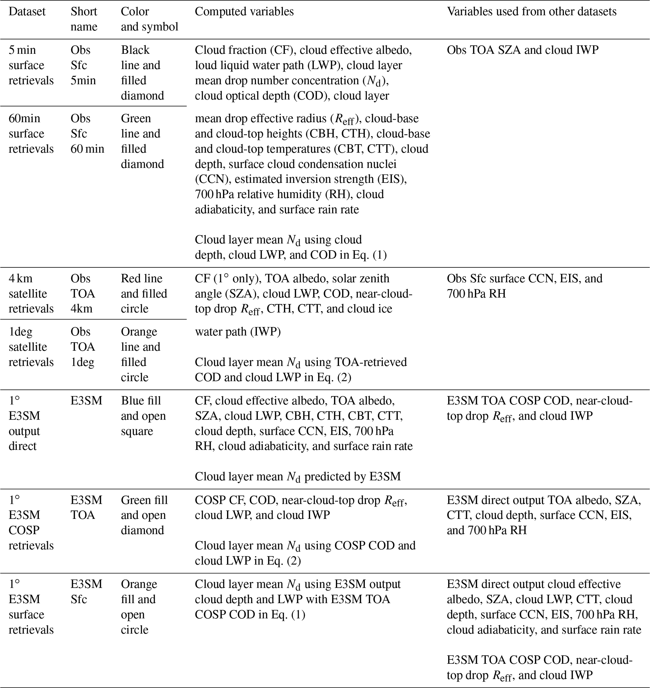
Several methodological decisions are made to improve the interpretability of model–observation comparisons in this study. Both surface and satellite observational retrievals of cloud properties are used in comparisons with model output because of uncertainties associated with each, for N_d in particular (Grosvenor et al., 2018). Although in situ cloud droplet measurements are more accurate than remote sensing retrievals, they are much rarer, which results in sampling biases. Surface and satellite retrievals are also applied to model output to yield multiple model datasets. Observational retrievals are analyzed at their highest resolution (5 min and 4 km) as well as coarse resolutions (60 min and 1^∘) consistent with model output. This approach yields four observational and three E3SMv1 datasets described in more detail below and in Table 1, where the output spread among them can be viewed as a rough measure of uncertainty stemming from retrieval assumptions and resolution. Lastly, analyses are confined to situations with single-layer liquid clouds and greater than 95 % cloud fraction to improve the accuracy of remote sensing retrievals (see, e.g., Grosvenor et al., 2018).

Table 1Each dataset analyzed including its short name and color used in figures along with variables computed by each dataset that are used in comparisons. Inputs used to compute cloud layer mean N_d for each dataset are listed. Variables within each dataset that are obtained from a different dataset are also shown.

Download Print Version | Download XLSX

Long-term surface retrievals require a fixed site that experiences frequent marine liquid clouds with aerosol, cloud, and atmospheric state measurements. They have several advantages over satellite retrievals including CCN observations that eliminate the need to use column-integrated optical properties, such as AOD or AI, and which are co-located with clouds rather than offset in space. In addition, no cloud adiabaticity assumption is required for retrieving N_d. Instead, adiabaticity can be estimated, and variables such as cloud depth and rain rate can be well quantified. This approach lends itself to Eulerian climatological statistics as opposed to Lagrangian trajectory analyses (e.g., Pincus et al., 1997; Johnson et al., 2000; Eastman et al., 2016; Goren et al., 2019; Mohrmann et al., 2019; Christensen et al., 2020, 2023) or comparisons of situational aerosol plume effects on clouds from ship tracks, volcanoes, or other significant emission sources (see Christensen et al., 2022, and references therein), though those strategies provide valuable complementary perspectives.

2.2 Observations

Surface datasets from 2016–2020 are collected from the ARM ENA site located on Graciosa Island in the Azores at about 39^∘ N and 28^∘ W (Mather and Voyles, 2013). The site experiences a range of marine midlatitude meteorological and cloud conditions (Dong et al., 2014; Rémillard and Tselioudis, 2015) with frequent drizzling stratocumulus (Rémillard et al., 2012; Giangrande et al., 2019; Jensen et al., 2021). Synoptic conditions strongly modulate clouds at ENA with substantial interannual variability, seasonal shifts in the Azores high and Icelandic low (Wood et al., 2015; Mechem et al., 2018), and frequent cold frontal passages (Naud et al., 2018; Kazemirad and Miller, 2020; Lamer et al., 2020; Ilotoviz et al., 2021). Mesoscale moisture variability in the boundary layer has also been shown to be important (Cadeddu et al., 2023), while interactions between cloud-top radiative cooling, drizzle evaporation, downdrafts, and boundary layer turbulence also affect the evolution of cloud properties (Ghate and Cadeddu, 2019; Ghate et al., 2021). In addition, cloud properties at ENA experience a diurnal cycle with cloud deepening and drizzle production overnight (Rémillard et al., 2012; Dong et al., 2014; Ghate et al., 2021). Such processes have been shown to modulate the effects of aerosols on cloud microphysical and radiative properties (Zheng et al., 2022; Qiu et al., 2023). Despite the importance of this meteorological regime for climate prediction, few long-term surface-based and in situ measurements targeting aerosol, cloud, and radiation conditions exist for it outside the ENA site, making it ideal for this study of aerosol effects on single-layer liquid clouds (Wood et al., 2015) and for assessing findings based on satellite remote sensing retrievals.

Surface CCN concentration at 0.2 % supersaturation is estimated by a CCN counter (ARM user facility, 2016a) that varies supersaturation set points between 0 % and 1 % over the course of an hour from which a polynomial is fit to the data to provide the CCN spectra as a function of supersaturation (ARM user facility, 2016b). Although aerosol measurements at ENA are occasionally impacted by emissions from the airport where the site is located (Gallo et al., 2020), this had a minimal impact on hourly 0.2 % CCN statistics, and thus we do not control for it. However, there are missing CCN measurements before 23 June 2016, between 31 July and 4 December 2018, and after 28 October 2020. Thus, analyses involving CCN cover a shorter period than the full 5 years. Cloud LWP is retrieved from a three-channel microwave radiometer (Turner et al., 2007; Cadeddu et al., 2013; ARM user facility, 2014c) with an estimated uncertainty of ∼20 g m⁻² for low LWPs increasing to ∼10 % for large LWPs (Cadeddu et al., 2013). A multifrequency shadowband radiometer (MFRSR) is used to retrieve cloud optical depth (COD) and layer mean effective radius (R_eff) (Min and Harrison, 1996; Min et al., 2003; ARM user facility, 2014a). Times for which the R_eff retrieval fails have a default constant R_eff value, and these times are removed from analyses. Cloud-base and cloud-top heights are retrieved from the Active Remote Sensing of Clouds (ARSCL) product (Clothiaux et al., 2000; ARM user facility, 2015) that combines vertically pointing ceilometer and Ka-band zenith radar (KAZR) measurements. Cloud-base and cloud-top temperatures are then estimated by matching temperature profiles retrieved from interpolated radiosonde measurements scaled by microwave radiometer precipitable water retrievals (Fairless et al., 2021; ARM user facility, 2013a) to cloud-base and cloud-top heights. Surface rain rates are retrieved using a Parsivel² disdrometer (ARM user facility, 2014b) and optical rain gauge (ARM user facility, 2013c). All-sky and clear-sky downwelling broadband shortwave irradiances are obtained from a pyranometer via the RADFLUX product (Long and Ackerman, 2000; ARM user facility, 2013c), from which cloud effective albedo is computed by dividing the downwelling broadband shortwave flux by the estimated clear-sky downwelling broadband shortwave flux. These variables are then either averaged or interpolated to 5 and 60 min intervals depending on whether the temporal frequency of the variable is less than or greater than that interval. N_d is then derived using MWR-derived LWP and MFRSR-derived COD as in McComiskey et al. (2009) with Eq. (1):

\begin{matrix} (1) & N_{d} = \frac{2^{- \frac{5}{2}}}{k H} {(\frac{4 π ρ_{liq}}{3 LWP})}^{2} {(\frac{5 C O D}{3 π Q})}^{3}, \end{matrix}

where H is the cloud depth, k is the ratio of the drop volume mean radius to R_eff, Q is the droplet scattering efficiency, and ρ_liq is the liquid water density. This retrieval assumes a stratified adiabatic cloud model as in Bennartz (2007) but allows for variable cloud adiabaticity by incorporating H following Boers and Mitchell (1994). LWP, COD, and H inputs from surface retrievals are averaged to 5 and 60 min intervals for each of the surface observation datasets (“Obs Sfc 5 min” and “Obs Sfc 60 in” in Table 1). While it is more physically realistic to compute N_d at the highest resolution possible and average it to coarser scales, that would be inconsistent with the E3SM-simulated surface retrievals that use inputs from a 1^∘ grid. We assume Q=2 following Bennartz (2007) and k=0.74 following Brenguier et al. (2011). Values for k commonly vary between 0.5 and 0.9 depending on the drop size distribution, which introduces uncertainty into the N_d retrieval. Adiabatic LWP (LWP_ad) is estimated by moist adiabatic ascent of a parcel with the retrieved cloud-base temperature and pressure to the radar-retrieved cloud top, from which cloud adiabaticity is computed as $α = \frac{LWP}{{LWP}_{ad}}$ . Lastly, CF is estimated from the frequency of clouds overhead within 5 and 60 min periods as detected in the ARSCL product.

Hourly satellite-based cloud retrievals are obtained from the NASA Visible Infrared Solar-infrared Split-Window Technique (VISST) dataset (Minnis et al., 2008, 2011; ARM user facility, 2013b, 2014c, 2018a, b). These retrievals use MeteoSat 10 and 11 geostationary satellite measurements to estimate top-of-atmosphere (TOA) radiative fluxes including all-sky albedo, cloud LWP and IWP, COD, and cloud-top R_eff, height, and temperature for 4 km wide pixels and 0.5^∘ regions, with the 0.5^∘ retrievals including CF. To match the E3SMv1 1^∘ grid, the 0.5^∘ retrievals are averaged to 1^∘ grids with each 0.5^∘ value weighted by CF for CF-dependent variables to yield in-cloud rather than all-sky values. From these, cloud layer mean N_d values for 4 km and 1^∘ grids in the “Obs TOA 4 km” and “Obs TOA 1^∘” datasets (Table 1) are retrieved using Eq. (2) following Bennartz (2007):

\begin{matrix} (2) & N_{d} = \frac{\sqrt{α Γ_{ad}}}{k} {(\frac{4 π ρ_{liq}}{3})}^{2} {(\frac{5 COD}{3 π Q})}^{3} (2 LWP)^{- \frac{5}{2}}, \end{matrix}

where α is cloud adiabaticity (assumed to be 0.8 in this study) and Γ_ad is the adiabatic liquid water content lapse rate. Equation (2) assumes adiabatically stratified clouds and uses inputs of COD, LWP, and cloud-top temperature (for calculation of Γ_ad) that are obtained from the VISST retrievals. Because α is assumed to be constant, this retrieval may be less accurate than the surface-based retrieval using Eq. (1), though the accuracies of COD and LWP inputs also matter. Bennartz (2007) showed that the uncertainty in this retrieval is less than 80 % for LWP exceeding 30 g m⁻² and CFs exceeding 0.8. Cloud adiabaticity is highly variable (e.g., Merk et al., 2016), which, along with the assumed k value of 0.74, cloud inhomogeneity, LWP uncertainty, and satellite viewing angle, contributes to N_d retrieval uncertainty. Grosvenor et al. (2018) reported N_d retrieval uncertainties of 54 %–78 % depending on the averaging area for ideal conditions, while Gryspeerdt et al. (2022) report lower uncertainties of 30 %–50 % for overcast stratocumulus with parameter thresholds to remove likely biased samples, most of which we employ in this study (see Sect. 2.4). Surface-measured CCN is interpolated to satellite retrieval times for analyses relating satellite-retrieved cloud properties with CCN concentration. An example of a closed-cell stratocumulus case is shown to highlight some of the key retrieved variables from the surface and satellite data (Fig. 1).

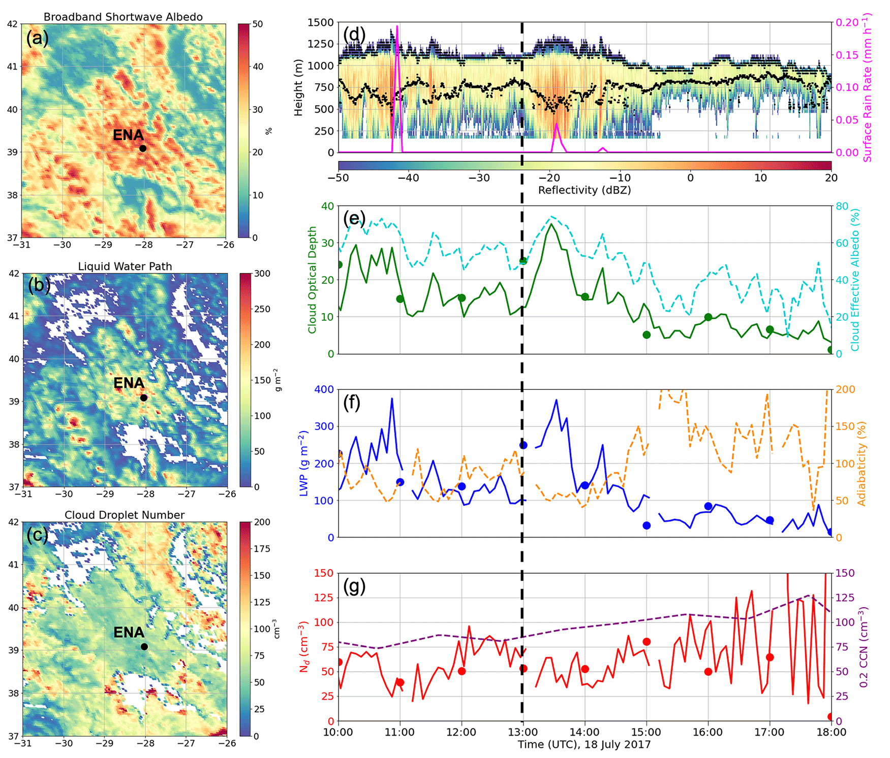
https://acp.copernicus.org/articles/23/13523/2023/acp-23-13523-2023-f01

Figure 1An example single-layer liquid cloud case at the ARM ENA site showing snapshots of 4 km satellite-retrieved (a) TOA albedo, (b) LWP, and (c) N_d at 13:00 UTC on 18 July 2017. An 8 h period of the same event is shown with surface observations of (d) Ka-band reflectivity and lidar-retrieved cloud base with 5 min optical rain gauge surface rain rate, (e) 5 min surface-retrieved COD (solid) and cloud effective broadband shortwave albedo (dashed), (f) 5 min LWP (solid) and cloud adiabaticity (dashed), and (g) 5 min N_d (solid) and hourly 0.2 % CCN concentration (dashed). Satellite-retrieved COD, LWP, and N_d values are plotted on the time series with circles. The dashed vertical black line indicates the time of the satellite snapshots. The surface site is noted in the satellite images.

Download

2.3 Model output

The E3SMv1 (Golaz et al., 2019) Atmosphere Model (Rasch et al., 2019) is run with ne30np4 horizontal resolution (approximately 1^∘ grid spacing) for 2016–2020 with hourly output. Although E3SMv2 was recently released (Golaz et al., 2022), E3SMv1 is used because it has been better characterized to date in many studies and as part of the Coupled Model Intercomparison Project Phase 6 (CMIP6; Eyring et al., 2016). Large-scale meteorological conditions are constrained via nudging the horizontal winds toward the Modern-Era Retrospective Analysis for Research and Applications version 2 (MERRA-2) (Gelaro et al., 2017) with a relaxation timescale of 6 h. Several of the variables used in analyses are directly outputted including grid-scale LWP, CF by height, surface and TOA radiative fluxes, temperature and moisture by height, surface rain rate, and surface CCN concentration at 0.2 % supersaturation.

Other variables require derivation. TOA albedo is computed as the upwelling broadband shortwave radiative flux divided by the downwelling broadband shortwave radiative flux at TOA. Cloud effective albedo is computed as the downwelling broadband shortwave radiative flux divided by the clear-sky broadband shortwave radiative flux at the surface. Cloud-base height is derived by summing height levels at which CF is greater than 0 weighted by that level's CF contribution minus the integrated CF below that level to the total 2D low-level CF moving upward from the surface until the 2D low-level cloud fraction is reached. This assumes maximum cloud overlap. Mathematically, this is written as

\begin{matrix} (3) & \begin{aligned} Cloud - base height = \sum_{z = 1}^{n_{lev}} \\ \{Z_{z} \max [\frac{{CF}_{z} - \max ({CF}_{1}, \dots, {CF}_{k - 1})}{\max ({CF}_{1}, \dots, {CF}_{n_{lev}})}, 0]\}, \end{aligned} \end{matrix}

where z is the height level with 1 being the lowest level and n_lev being the highest level, Z_z is the height at level z, and CF_z is the cloud fraction at level z. As an example, if the 2D low-level cloud fraction is 80 %, the lowest-level clouds are located at 1000 m with a CF of 60 %, and the next height level at 1200 m has a CF of 80 % that is equal to the low cloud fraction, the cloud-base level would be $(60 / 80) \cdot 1000$ m + $((80 - 60) / 80) \cdot 1200$ m = 1050 m. However, a complication arises due to limited model vertical resolution. The existence of cloud at a point means that the cloud layer thickness is equal to the distance between the model half-levels bounding the point, but if the cloud was fully resolved, it could be anything greater than 0 up to this value. To account for this effect in comparisons to observations, cloud bases are computed separately using both the half-levels directly below the cloud mass levels and using the cloud mass levels, and then these values are averaged as a best estimate. The same method is applied for estimating cloud-top heights but integrating normalized CF-weighted height levels downward from above cloud top until the 2D low-level cloud fraction is consumed. Cloud-base and cloud-top temperatures are computed in the same way. The cloud layer mean N_d is computed by averaging N_d at each level in the cloud weighted by the CF at that level. Note that this is the grid-scale “stratiform” N_d, whereas LWP and CF include convective contributions to be consistent with observations. This cloud layer mean N_d is used in a dataset referred to as “E3SM” (see Table 1), whereas two additional model datasets are constructed to mimic TOA and surface observational retrievals, respectively.

The TOA-based N_d retrieval used in the “E3SM TOA” dataset (Table 1) leverages simulated MODerate resolution Imaging Spectroradiometer (MODIS) retrievals (Pincus et al., 2012) using the Cloud Feedback Model Intercomparison Project Observation Simulator Package (COSP; Bodas-Salcedo et al., 2011) version 2 (Swales et al., 2018). The simulator reads in E3SMv1 vertical profiles of layer COD and R_eff for liquid and ice from which MODIS TOA visible and near-infrared radiances are estimated. R_eff is determined from the two-moment parameterized cloud droplet size distribution in the Morrison–Gettelman (MG2) microphysics scheme (Morrison and Gettelman, 2008; Gettelman and Morrison, 2015; Gettelman et al., 2015). From these inputs and predicted radiances, 2.1 µm R_eff as estimated from a TOA perspective is predicted, from which the product of COD and R_eff is used to estimate LWP (Pincus et al., 2012). Simulated MODIS-retrieved LWP and COD with cloud-top temperature are used to derive N_d following Eq. (2) in Sect. 2.1 that is also used for observational TOA retrievals. The simulated surface-based N_d retrieval used in the “E3SM Sfc” dataset (Table 1) uses vertically integrated cloud plus rainwater content (since surface-based observations are also impacted by rain) with COSP-simulated COD and cloud depth following Eq. (1) in Sect. 2.1 that is also used for surface-based observations. Cloud adiabaticity is also computed following the same method used for observations in Sect. 2.2 by dividing LWP by the adiabatic LWP estimated from moist adiabatic ascent from cloud base to top.

To summarize the differences between the three E3SM datasets used in comparisons (E3SM, E3SM Sfc, and E3SM TOA) as highlighted in Table 1, E3SM Sfc uses direct model output like E3SM but with N_d retrieval following the surface-based N_d retrieval for observations with directly predicted LWP and cloud depth coupled with COD obtained from COSP. E3SM TOA uses the same COSP COD as input to its N_d retrieval but further uses LWP from the COSP MODIS simulator as input with a constant cloud adiabaticity of 0.8 following TOA-based observational retrievals. E3SM-predicted R_eff and COD vertical profiles are inputs to the COSP MODIS simulator. However, LWP is predicted by the COSP MODIS simulator based on R_eff and COD inputs, whereas LWP for E3SM and E3SM Sfc datasets is predicted and not linked by a simple adiabatic droplet growth model to R_eff and COD. Thus, the relationship between COD, LWP, R_eff, and N_d differs between datasets due to differing LWP inputs and N_d retrieval assumptions, which motivates the usage of multiple retrievals with direct model output for better interpretable comparisons with observational retrievals.

2.4 Comparison methods

All datasets and variables used in comparisons are listed in Table 1 including 5 and 60 min averaged surface observations (Obs Sfc 5 min, Obs Sfc 60 min), 4 km and 1^∘ satellite observations (Obs TOA 4 km, Obs TOA 1^∘), and E3SMv1 datasets that use direct output (E3SM), surface-estimated N_d (E3SM Sfc), and TOA-estimated N_d (E3SM TOA). For both observations and E3SM, the surface N_d retrieval (Eq. 1) is the same as the TOA N_d retrieval (Eq. 2) except that (i) no cloud adiabaticity assumption is made and (ii) the sources for LWP and COD inputs to Eqs. (1) and (2) differ (Table 1). Effects of assuming constant adiabaticity on cloud susceptibilities are explored in analyses by making use of surface retrieval sensitivity tests. These tests still use surface-retrieved COD and LWP for observations and COSP COD and model-predicted LWP for E3SM when computing N_d but use Eq. (2) rather than Eq. (1) with adiabaticity assumed to be constant at 80 % to match TOA datasets. Although it would be ideal to apply a parameterization for adiabaticity within TOA retrievals to potentially improve their accuracy, deriving such a parameterization is beyond the scope of this study. The sensitivity tests are instead simply meant to quantify differences between constant and variable adiabaticity representations in retrievals. How cloud adiabaticity is handled in retrievals will be shown to be a key factor in understanding differences between the various model and observation datasets.

LWP estimates also slightly differ between the three E3SMv1 datasets. To be consistent with surface measurements, E3SM surface retrievals use total LWP inclusive of rain and convective liquid from the Zhang–McFarlane (Z–M) scheme (Zhang and McFarlane, 1995) that accounts for 15 % of the total LWP in single-layer liquid cloud situations at ENA. The direct output E3SM dataset uses summed column-integrated grid-scale and Z–M cloud water (not including rainwater path), and TOA retrievals use COSP-simulated LWP. Times with drizzle can influence the accuracy of retrievals (Cadeddu et al., 2020) but are not removed except for surface-based observations when drizzle at the surface is sufficient to obscure MWR LWP retrievals. For some variables such as albedo, CCN concentration, COD, and R_eff, the value from a single dataset is used for the others that do not have uniquely derived values (rightmost column in Table 1). For these variables, only differing sampling constraints produce slight differences in values between datasets. Since only overcast conditions are analyzed, all-sky albedo varies as cloud albedo varies, and thus we use all-sky values in analyses to avoid estimating clear-sky contributions.

Comparisons between E3SMv1 and observational datasets are confined to specific situations to limit sources of retrieval uncertainty and possible contributors to dataset differences. All comparisons are limited to the column over the ENA site. In E3SMv1 datasets, single-layer liquid cloud situations are isolated by removing times with COSP-simulated MODIS IWP > 0 or cloud-top temperature < 0 ^∘C. E3SMv1-predicted IWP is not used since it is commonly slightly greater than 0. This same IWP and cloud-top temperature filtering is applied to VISST datasets, which allows multiple liquid cloud layers to exist due to a lack of sufficient TOA data to remove such situations. However, surface-based vertically pointing radar measurements indicate that such situations are not common for the overcast, liquid cloud situations considered. For surface-based observations, only single-layer cloud situations are considered, and situations with cloud-top temperature < 0 ^∘C are removed using the radar-detected cloud boundaries described in Sect. 2.2. Only situations with CF > 95 %, solar zenith angle (SZA) < 65^∘, LWP > 20 g m⁻², and COD > 4 are included following some recommendations in Grosvenor et al. (2018) and Gryspeerdt et al. (2022). E3SMv1 and TOA measurements of these variables are spatial averages, whereas surface measurements of these variables are averaged over 5 and 60 min periods. For analyses relating cloud properties to surface CCN concentrations, only times with cloud-base potential temperature < 2 ^∘C warmer than the near-surface potential temperature are included. These are situations that are most likely to have surface-coupled cloud bases that respond to surface CCN more strongly than decoupled clouds (Dong et al., 2015). This threshold will not remove all uncoupled clouds, but it allows for retaining greater sample sizes. Other cloud–surface coupling indices produced similar results as the potential temperature metric (Fig. S1 in the Supplement). Lastly, Graciosa Island where the ENA site is located is not represented in the E3SMv1 simulation but has been shown to influence the boundary layer vertical motion and turbulence at the site when wind directions are between 90 and 310^∘ where 0^∘ is from the north (Ghate et al., 2021; Jeong et al., 2022). It is also possible for the terrain on the island, which reaches 400 m a.s.l., to influence clouds. Such potential island effects have not been removed from analyses to retain sufficient sampling but could contribute to some of the differences between observations and E3SMv1.

3 Cloud, aerosol, radiation, and atmospheric state properties

The sampling of overcast single-layer liquid clouds at ENA depends on the resolution and sensitivity of each dataset. The average warm, liquid CF and percentage of times with CF > 95 % for times without supercooled and ice clouds are greater for the 5 min surface and 4 km TOA retrievals than the 60 min surface and 1^∘ TOA retrievals (Table 2). This is likely the result of increasing probability of encountering overlying cloud layers as the scale increases. The average warm, liquid CF in E3SMv1 for times without overlying clouds is slightly lower than observed. However, the percentage of time that CF exceeds 95 % is similar for satellite-observed and COSP-simulated TOA estimates (20 % vs. 23 %) with the 60 min surface estimate a bit lower (17 %) and direct model output having a greater occurrence (31 %). SZA, LWP, and COD constraints further reduce observational hourly sampling to between 649 and 1381 with between 1697 and 1941 hourly E3SM samples depending on the dataset. Analyses involving surface CCN concentration have even fewer samples. This is partly because of the surface coupling constraint, though observed samples drop further than for E3SM due to some missing and bad CCN data, resulting in 197–328 hourly observational samples but 1303–1459 E3SM samples.

Table 2Warm (T≥0 ^∘C) liquid cloud fraction and sampling as filters are applied for each dataset for only situations with no sub-freezing clouds detected using both IWP and cloud-top temperature constraints. For E3SM, IWP is derived from the COSP simulator due to an abundance of very low ice concentrations in the upper troposphere that would remove too many warm, liquid cloud samples. Sensitivity tests indicate that these low ice concentrations that COSP does not detect have little impact on albedo. For non-TOA datasets, multi-layer warm cloud situations have additionally been removed. The Obs TOA 4 km CF is derived from measurements over a 0.5^∘ region.

Download Print Version | Download XLSX

For times with overcast, warm liquid clouds and sufficient SZA, distributions of TOA albedo, cloud effective albedo at the surface, and COD are shown in Fig. 2. E3SMv1 has slightly greater median TOA albedos than observed (Figs. 2a and 3), though median surface-estimated cloud effective albedos are slightly lower (Figs. 2b and 3). This TOA difference will be shown later to be the result of differing SZA–N_d correlations between E3SMv1 and observations. Indeed, median COD is similar between E3SMv1 and TOA observations (Fig. 3). Surface-estimated COD values are greater than simulated, consistent with greater cloud effective albedos caused by greater LWPs being sampled with similar N_d values (Figs. 3 and 4a, b). Median LWP is lower in E3SMv1 compared to observations (Figs. 3 and 4a) by ∼30 % (62–68 g m⁻² vs. 78–92 g m⁻²). Unlike LWP, N_d is notably greater in E3SMv1 TOA than TOA observations (95 cm⁻³ vs. 56–61 cm⁻³ medians; Figs. 3and 4b) and droplet R_eff is notably smaller (9.6 µm vs. 13 µm median values; Figs. 3 and 4c), though E3SMv1 directly outputted N_d is lower with a median value of 70 cm⁻³. While surface-retrieved R_eff observations are also greater than simulated, 60 min surface-retrieved N_d observations are similar to E3SMv1 surface-retrieved N_d, both having median values near 110 cm⁻³ (Figs. 3 and 4b, c), while 0.2 % surface CCN concentration distributions are also similar (Figs. 3 and 4d). Model–observation N_d comparisons clearly depend tremendously on how N_d is retrieved with typical values changing by up to a factor of 2 based on retrieval method. Simulated N_d values via TOA retrievals that are greater than directly outputted by E3SMv1 are consistent with results in Saponaro et al. (2020) for different Earth system models. This emphasizes the importance of using multiple different retrievals to assess and better interpret model–observation differences.

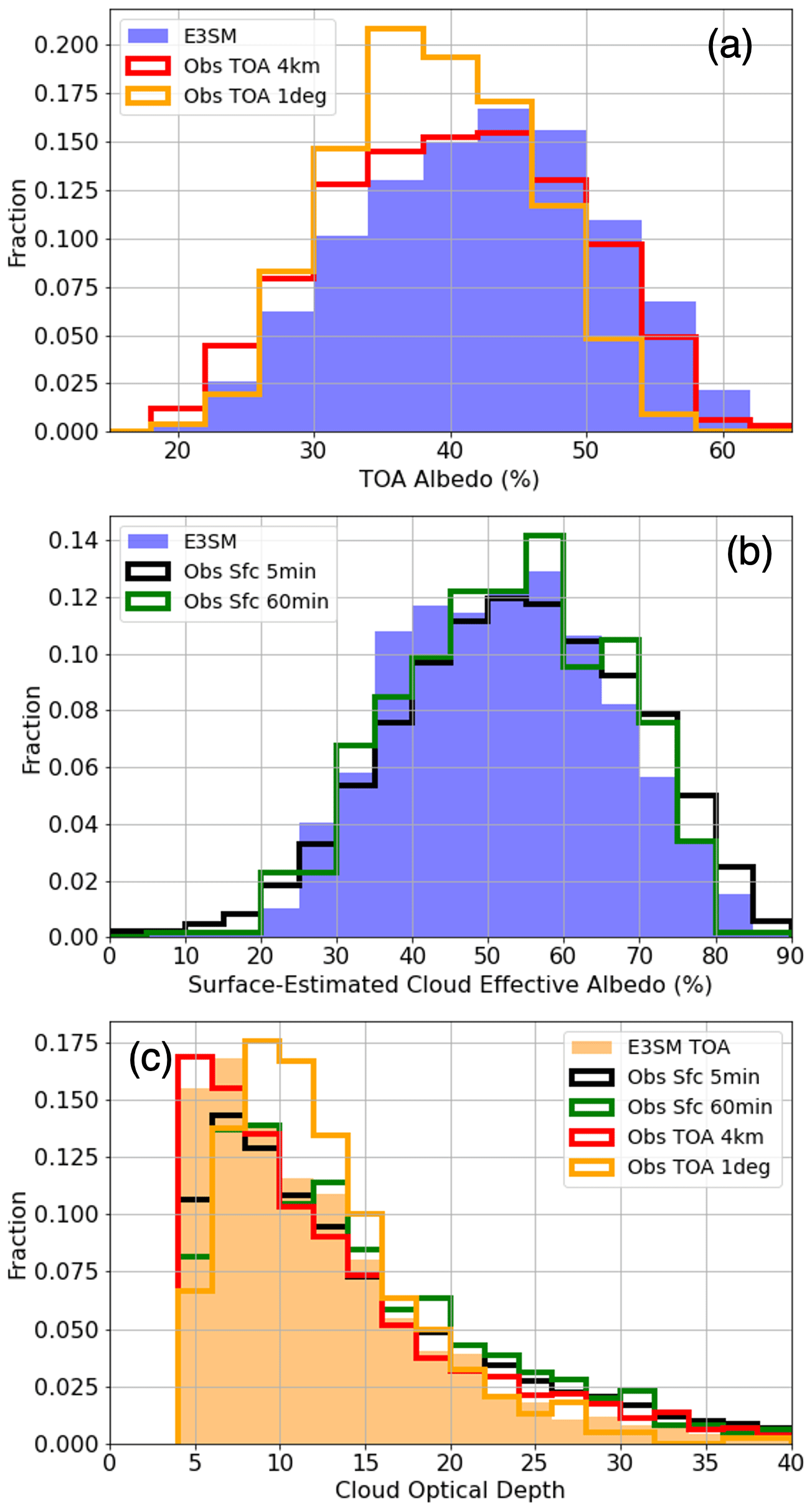
https://acp.copernicus.org/articles/23/13523/2023/acp-23-13523-2023-f02

Figure 2Probability distributions of observed and simulated (a) TOA albedo, (b) surface-estimated cloud effective albedo, and (c) cloud optical depth. Datasets are excluded when they are similar to another already shown due to being derived from the shown dataset.

Download

https://acp.copernicus.org/articles/23/13523/2023/acp-23-13523-2023-f03

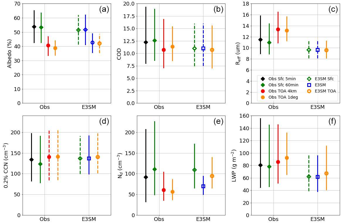
Figure 3Median (symbol) and interquartile range (vertical bar) values of key variables: (a) albedo, (b) COD, (c) R_eff, (d) 0.2 % CCN, (e) N_d, and (f) LWP. Dashed vertical bars indicate datasets sampled from solid vertical bar datasets including Obs TOA from Obs Sfc CCN values, E3SM and E3SM Sfc COD and R_eff from E3SM TOA, E3SM Sfc and TOA albedos and CCN from E3SM, and E3SM Sfc LWP from E3SM.

Download

https://acp.copernicus.org/articles/23/13523/2023/acp-23-13523-2023-f04

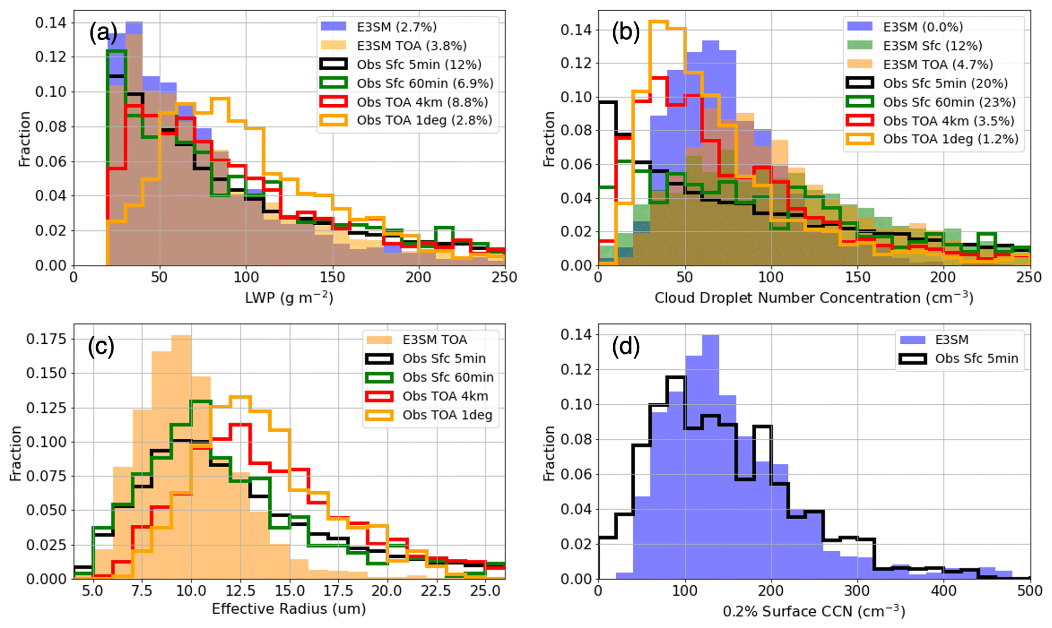
Figure 4Probability distributions of observed and simulated (a) cloud LWP, (b) cloud layer mean N_d, (c) cloud droplet R_eff, and (d) 0.2 % surface CCN. Percentages in the legends indicate how many samples exceed the range of the x axis. Datasets are excluded when they are similar to another already shown due to being derived from the shown dataset.

Download

For overcast cloud conditions at ENA, E3SMv1 has weaker than observed inversion strengths and higher than observed above-inversion relative humidity (Fig. 5a and b). Even though the simulation winds are nudged to MERRA-2, thermodynamic state is not and can develop errors. These errors suggest excessive mixing between the boundary layer and free troposphere or insufficient free-tropospheric subsidence. Zheng et al. (2020) found insufficient vertical mixing in E3SMv1 for the subtropical stratocumulus-to-cumulus transition region of the northeastern Pacific, but Ma et al. (2022) found excessive turbulent mixing in E3SMv1 that has been tuned down in E3SMv2 (Golaz et al., 2022). These inversion differences are associated with clouds in E3SMv1 that have similar cloud bases to observed (Fig. S2a and b) but higher and colder cloud tops (Fig. S2c and d) with greater cloud depths (Fig. 5c). TOA estimates of cloud depth are shallower than in surface retrievals and E3SM direct output due to assuming that clouds are 80 % adiabatic, whereas most clouds have less cloud adiabaticity, particularly in E3SM (Fig. 5d). Note that observationally estimated adiabaticities can exceed 100 % and even approach 200 % (Fig. 1). This typically occurs for thin clouds with low LWP values for which the LWP and cloud depth retrieval errors can cause adiabaticity errors on the order of 100 %. However, most of the sampled observed clouds are subadiabatic, consistent with the results of Wu et al. (2020b), with a mean of 71 % that is only slightly higher than the 63 % found in Merk et al. (2016) and not far below the 80 % assumed in TOA retrievals. However, E3SMv1's mean adiabaticity is 27 %, a much lower value than observed that is associated with its deeper clouds and weaker inversions but similar LWPs. A total of 68 % of simulated clouds have an adiabaticity < 30 %, whereas only 16 % do in observations (Fig. 5d). On the other hand, 64 % of observed clouds are more than 60 % adiabatic but only 12 % of clouds sampled in E3SMv1 reach this threshold. Thus, an assumption of 80 % adiabaticity for E3SM clouds is substantially biased high. The differences in how cloud adiabaticity is handled across the datasets will be shown to impact quantification of susceptibilities.

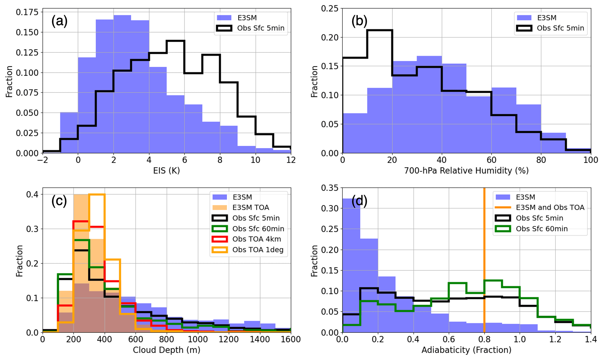
https://acp.copernicus.org/articles/23/13523/2023/acp-23-13523-2023-f05

Figure 5(a) Estimated inversion strength (EIS), (b) 700 hPa RH, (c) cloud depth, and (d) cloud adiabaticity probability distributions for E3SM and observations. Observations are derived from interpolated radiosondes. Datasets are excluded when they are similar to another already shown due to being derived from the shown dataset.

Download

4 Cloud albedo susceptibility

Differences in observed and simulated cloud properties can result from differences in atmospheric states and/or errors from subgrid-scale parameterizations. Such errors do not necessarily imply that the responses of clouds and radiation to aerosol perturbations are incorrect, and it is these responses that are the primary focus here. In particular, the response of cloud albedo to CCN is evaluated in this section. The cloud albedo (A) susceptibility to changes in CCN number concentration is evaluated by separating the Twomey effect and LWP response components with Eq. (4) (Quaas et al., 2008):

\begin{matrix} (4) & \frac{d A}{d \ln CCN} = (\frac{\partial A}{\partial \ln N_{d}} + \frac{\partial A}{\partial \ln LWP} \frac{d \ln LWP}{d \ln N_{d}}) \frac{d \ln N_{d}}{d \ln CCN} . \end{matrix}

Given the overcast cloud condition requirement, the CF response is neglected, and we analyze all-sky albedo for TOA relationships. COD susceptibility is also analyzed, for which A in Eq. (4) is simply replaced with lnCOD. Changes in the SZA affect A via changes in the slant path of shortwave radiation through the cloud, whereas COD estimates the vertical component of the change in shortwave radiation.

The following sections quantify the individual terms of Eq. (4) within each of the E3SMv1 and observation datasets within the context of retrieval uncertainties. Analyses are also performed to assess possible causes for model–observation discrepancies including differences in R_eff and cloud adiabaticity. Within the context of Eq. (4), R_eff is implicit since it is retrieved from only two variables (LWP and COD) for surface measurements, while for TOA measurements, COD and R_eff collectively determine LWP. These variables together also determine cloud layer mean N_d with an assumption of scaled adiabatic growth of droplets from cloud base to top. In E3SM, R_eff also only depends on two variables, the predicted LWC and N_d that dictate the two-moment cloud droplet size distribution. Thus, LWP and N_d encapsulate the information content available in the cloud retrievals. Surface retrievals of cloud depth provide additional information on the cloud adiabaticity, which scales adiabatic N_d and LWP by $\sqrt{α} N_{d, adiabatic}$ and αLWP_adiabatic, producing Eq. (5):

\begin{matrix} (5) & \begin{aligned} \frac{d A}{d \ln CCN} & = (\frac{\partial A}{\partial \ln (\sqrt{α} N_{d, adiabatic})} \\ + \frac{\partial A}{\partial \ln (α {LWP}_{adiabatic})} \frac{d \ln (α {LWP}_{adiabatic})}{d \ln (\sqrt{α} N_{d, adiabatic})}) \\ \frac{d \ln (\sqrt{α} N_{d, adiabatic})}{d \ln CCN} . \end{aligned} \end{matrix}

Hence, the magnitudes of terms can change based on the chosen constant α value, and because $0 < α \leq 1$ , LWP decreases faster than N_d from adiabatic values as α decreases. However, we will show that retrieved α is not constant and varies with N_d and LWP, which alters the magnitudes of terms further and will be shown to be important in understanding differences between datasets.

4.1 Twomey effect comparison

We first evaluate the Twomey effect signified by $\frac{\partial A}{\partial \ln N_{d}} \frac{d \ln N_{d}}{d \ln CCN}$ , which describes the response of albedo to a change in N_d via a change in CCN.

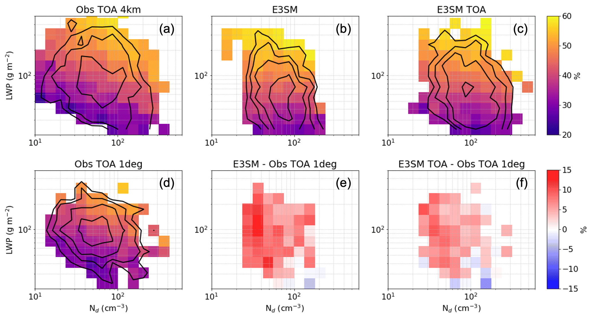
https://acp.copernicus.org/articles/23/13523/2023/acp-23-13523-2023-f06

Figure 6Median TOA albedo vs. N_d and LWP for (a) Obs TOA 4 km, (b) E3SM, (c) E3SM TOA, and (d) Obs TOA 1^∘. Absolute differences are also shown between (e) E3SM and Obs TOA 1^∘ and between (f) E3SM TOA and Obs TOA 1^∘. Black contours indicate sample size thresholds of 0.4 %, 0.8 %, 1.6 %, and 3.2 %.

Download

https://acp.copernicus.org/articles/23/13523/2023/acp-23-13523-2023-f07

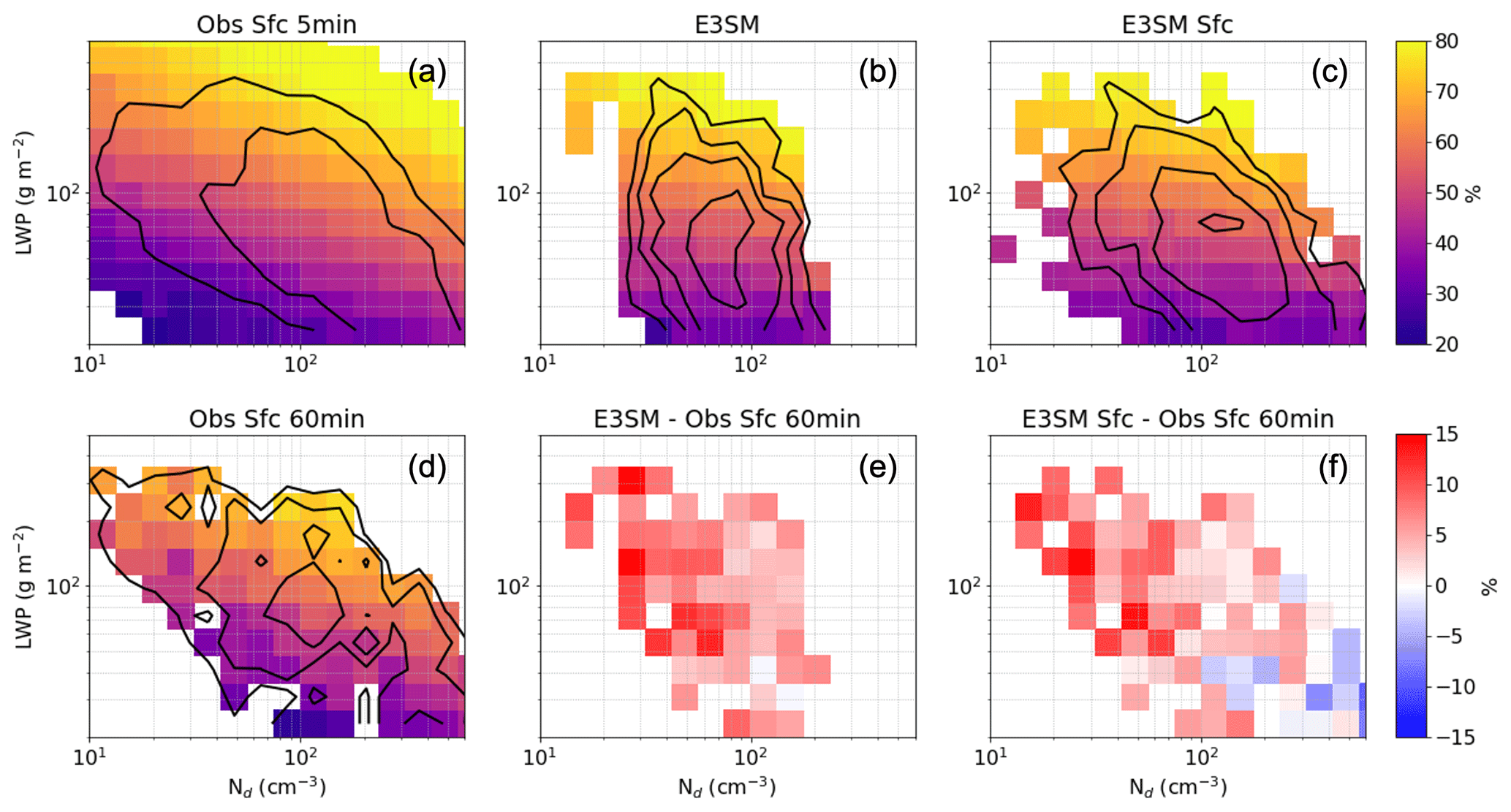
Figure 7Median cloud effective albedo vs. N_d and LWP for (a) Obs Sfc 5 min, (b) E3SM, (c) E3SM Sfc, and (d) Obs Sfc 60 min. Absolute differences are also shown between (e) E3SM and Obs Sfc 60 min and between (f) E3SM Sfc and Obs Sfc 60 min. Black contours indicate sample size thresholds of 0.4 %, 0.8 %, 1.6 %, and 3.2 %.

Download

https://acp.copernicus.org/articles/23/13523/2023/acp-23-13523-2023-f08

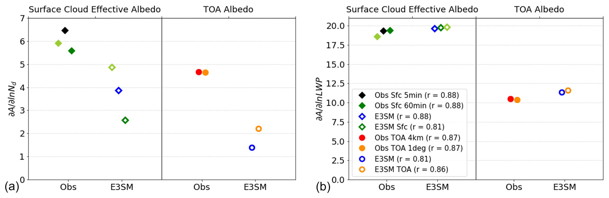
Figure 8Surface cloud effective albedo and TOA albedo as functions of (a) ln N_d and (b) lnLWP for observational and E3SM datasets. Estimates are obtained from ordinary least-squares multiple linear regression with Pearson correlation coefficients shown in the legend. Light-green symbols represent Obs Sfc 60 min and E3SM Sfc datasets with a recomputed N_d that assumes 80 % adiabaticity like the TOA retrievals.

Download

https://acp.copernicus.org/articles/23/13523/2023/acp-23-13523-2023-f09

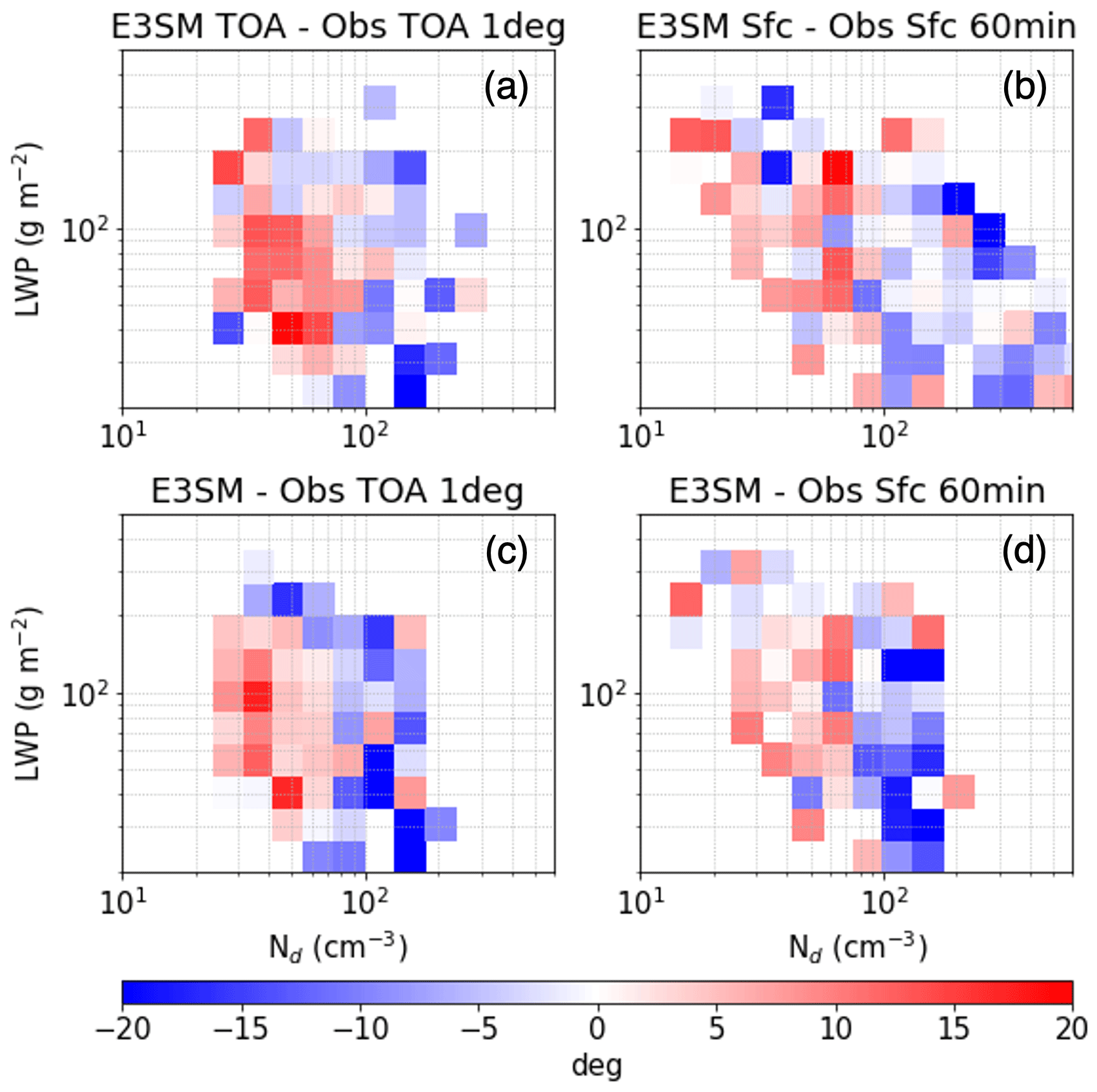
Figure 9Median absolute SZA differences between (a) E3SM TOA and Obs TOA 1^∘, (b) E3SM Sfc and Obs Sfc 60 min, (c) E3SM and Obs TOA 1^∘, and (d) E3SM and Obs Sfc 60 min as functions of N_d and LWP.

Download

4.1.1 Albedo dependence on droplet concentration

Isolating the Twomey effect requires accounting for the effect of changes in LWP on A. The effect of both LWP and N_d on A is visualized in Figs. 6a–d and 7a–d, which show heatmaps of median A within bins of N_d and LWP for the various datasets analyzed. All datasets show similar patterns with A increasing foremost with increasing LWP and secondarily with increasing N_d, though the A sensitivity to N_d is muted in E3SMv1, particularly for TOA estimates. Indeed, absolute differences between E3SMv1 and observations in Figs. 6e–f and 7e–f show that E3SMv1 A is much greater than observed for relatively low N_d values, a difference that decreases as N_d increases. $\frac{\partial A}{\partial \ln N_{d}}$ is further quantified by multiple linear regression. Regression coefficients confirm that $\frac{\partial A}{\partial \ln LWP}$ is greater than $\frac{\partial A}{\partial \ln N_{d}}$ by a factor of 2–8 depending on the dataset considered (Fig. 8). All dataset fits have Pearson correlation coefficients (r) of 0.81–0.88 (Fig. 8), showing that LWP and N_d alone predict much of the A variability. Consistent with Figs. 6 and 7, E3SMv1 coefficients have a similar response of A to LWP as observations but the response of A to N_d is about half that observed. The estimated response of A to N_d also depends on how N_d is retrieved. Whereas a surface-retrieved N_d value decreases $\frac{\partial A}{\partial \ln N_{d}}$ relative to the actual E3SMv1-predicted N_d value (green vs. blue open diamonds), a TOA-retrieved N_d does the opposite (orange vs. blue open circles) (Fig. 8). This difference is explained by differences in cloud adiabaticity assumptions made by TOA and surface retrievals. TOA retrievals assume an adiabaticity of 80 %, while surface retrievals allow adiabaticity to vary by leveraging cloud depth measurements. If N_d is recomputed from surface-retrieved COD and LWP assuming an adiabaticity of 80 % in Eq. (2), then the sensitivity of albedo to N_d increases (light-green relative to dark-green symbols in Fig. 8). The increase is especially dramatic for E3SMv1, where surface-retrieved $\frac{\partial A}{\partial \ln N_{d}}$ assuming 80 % adiabaticity now exceeds the value derived from direct model output in agreement with the higher TOA retrieval value relative to direct model output. Clearly cloud adiabaticity can affect $\frac{\partial A}{\partial \ln N_{d}}$ , a topic discussed further in the next section. While the resolution of the N_d retrieval input data does not affect TOA $\frac{\partial A}{\partial \ln N_{d}}$ , the surface $\frac{\partial A}{\partial \ln N_{d}}$ decreases by 15 % when switching from 5 to 60 min inputs, a difference that is less than the model–observation differences (Fig. 8). Thus, there is agreement between datasets that E3SMv1 significantly underestimates the N_d effect on A despite reasonable sensitivity of A to LWP.

4.1.2 Factors affecting model–observation differences

We first investigate how SZA impacts differences in observed and simulated $\frac{\partial A}{\partial \ln N_{d}}$ . SZA and N_d are not correlated in observations, but E3SMv1 SZA decreases as N_d increases (Fig. S3). This difference between E3SMv1 and observations is evident in Fig. 9 where E3SMv1 has greater SZA values for relatively low N_d and lower SZA values for relatively high N_d. We first check whether this correlation is caused by the diurnal cycle. There is an early-afternoon N_d minimum in E3SMv1 datasets (dashed lines in Fig. S4e) that correlates with an SZA minimum (Fig. S4b), whereas observed variables lack such a correlation. However, this is the opposite SZA–N_d correlation in Figs. S3 and 9, so this cannot be the cause of the SZA–N_d correlation in those figures. Surface CCN concentration reaches a minimum in early afternoon (Fig. S5a), which is less apparent in observations than E3SMv1 and could be the cause of the simulated early-afternoon N_d minimum. We next investigate the seasonal cycle. Simulated N_d strongly peaks in July with median values that are more than twice the wintertime minimum (Fig. 10e), a seasonal cycle that is anticorrelated with the SZA and A seasonal cycles (Fig. 10b and c). R_eff also exhibits a notable seasonal cycle, but LWP does not. Thus, seasonality is likely the cause of the E3SMv1 SZA–N_d correlation. Observations also exhibit N_d seasonality, consistent with past studies (e.g., Wood et al., 2015) but with a peak in May that does not correlate with the SZA seasonal cycle. Both E3SMv1 and observations also exhibit strong seasonal cycles in surface CCN concentration (Fig. S5b), and despite being constrained to specific cloud situations, the wintertime minimum and summer maximum in CCN concentration are consistent with the results of Zheng et al. (2018). The observed maximum is 2 months earlier than simulated, possibly contributing to the ∼2-month earlier peak in observed maximum N_d relative to E3SMv1 that leads to the differing relationship of N_d with SZA between E3SMv1 and observations.

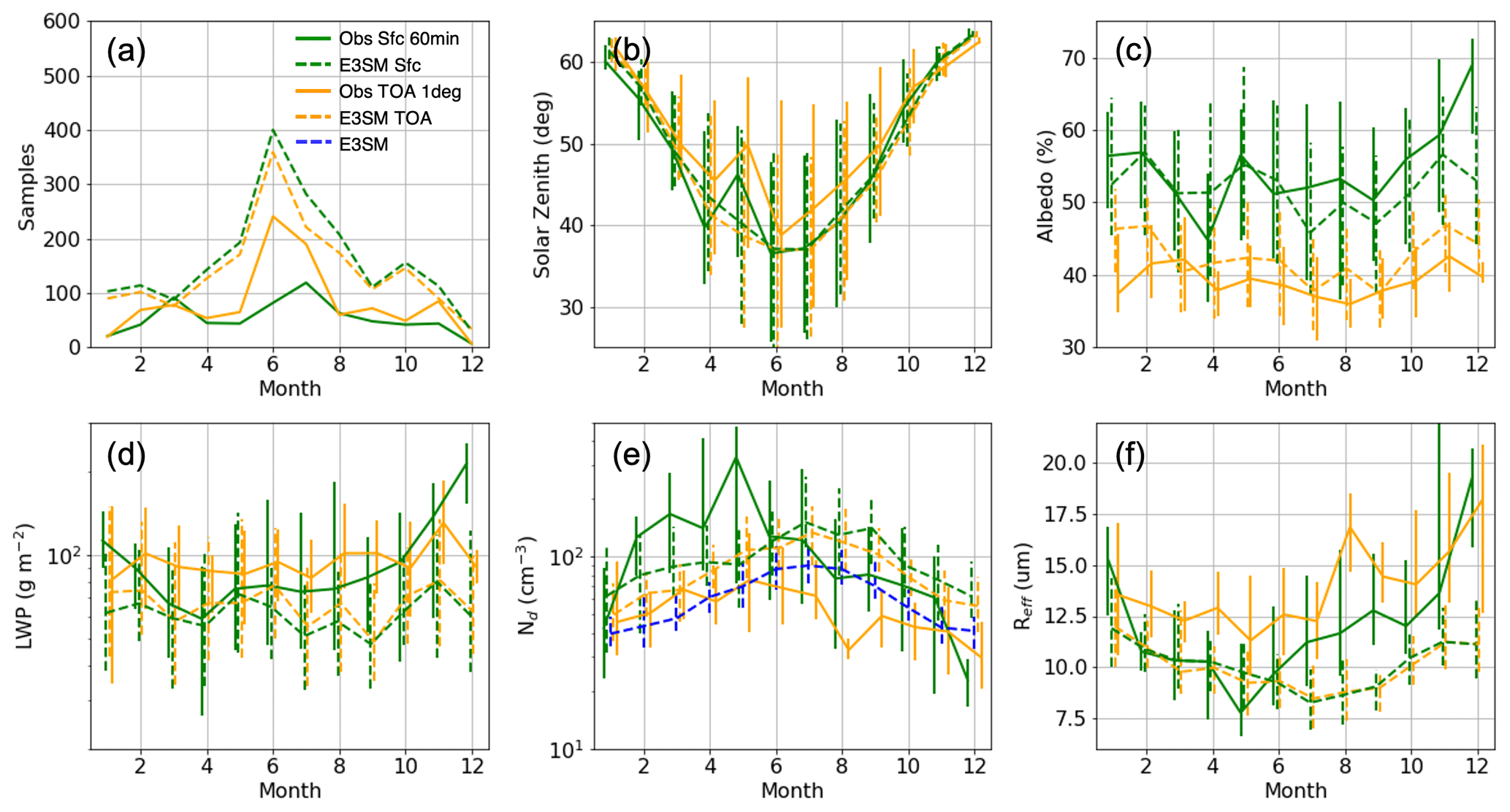
https://acp.copernicus.org/articles/23/13523/2023/acp-23-13523-2023-f10

Figure 10Seasonal cycles of (a) the number of samples and interquartile ranges (vertical bars) connected by medians for (b) SZA < 65^∘, (c) TOA or cloud effective albedo, (d) cloud LWP, (e) layer mean N_d, and (f) R_eff.

Download

Because seasonality-influenced SZA–N_d correlations significantly impact model–observation differences in cloud albedo susceptibility terms, we also analyze the COD response to N_d and LWP. COD is much less influenced by such correlations, which allows for better isolation of cloud radiative effects caused by N_d and LWP alone rather than SZA. Observed and simulated $\frac{\partial \ln COD}{\partial \ln LWP}$ values are similar, which is consistent with $\frac{\partial A}{\partial \ln LWP}$ comparisons (Fig. 11). Whereas observed and simulated $\frac{\partial A}{\partial \ln N_{d}}$ values significantly differed, observed and simulated $\frac{\partial COD}{\partial \ln N_{d}}$ values are much more similar (Fig. 11). The difference that remains is E3SM and E3SM Sfc values being less than surface-based observations. However, controlling for cloud adiabaticity differences between E3SM and observations removes this difference (light-green symbols in Fig. 11). As described in Sect. 4.1.1, this is done by recomputing N_d in surface retrievals with scaled cloud depths to values that would be associated with 80 % adiabatic LWP. This increases $\frac{\partial \ln COD}{\partial \ln LWP}$ by over 10 % for observations and almost 50 % for E3SMv1, leading to values that are almost identical to TOA-retrieved values that assume 80% adiabaticity. To visualize this, Fig. 12 shows absolute differences of lnCOD between E3SM and observational datasets as a function of LWP and N_d (lnCOD values for each dataset are shown in Fig. S6). Note that when the exact same retrieval with a constant adiabaticity is applied to both E3SM and observations (Fig. 12a and c), there is virtually no difference in lnCOD for a given LWP and N_d because N_d is computed from COD, LWP, and adiabaticity or cloud depth. When adiabaticity is not held constant, lnCOD values for surface-based retrievals in E3SMv1 and observations diverge (Fig. 12b). Why is this? As shown in Fig. 13, cloud adiabaticity is frequently lower than 80 % and decreases as N_d decreases and LWP increases. E3SMv1 also has many more subadiabatic clouds than observed. When N_d is recomputed using a constant adiabaticity, it causes a shift in the N_d distribution. For the case of constant 80 % adiabaticity, low N_d values with adiabaticity much less than 80 % increase more than higher N_d values that have higher adiabaticity values. This causes a narrowing of the ln N_d distribution, which increases $\frac{\partial \ln COD}{\partial \ln N_{d}}$ (Fig. 14). Because adiabaticity also decreases with increasing LWP, the shift in the ln N_d distribution varies by LWP (Fig. 14), causing a slight decrease in $\frac{\partial \ln COD}{\partial \ln LWP}$ (Fig. 11) that can also affect $\frac{\partial \ln COD}{\partial \ln N_{d}}$ . Thus, the grossly subadiabatic clouds in E3SMv1 suppress the change in COD with N_d relative to more adiabatic observed clouds and retrievals with constant 80 % adiabaticity.

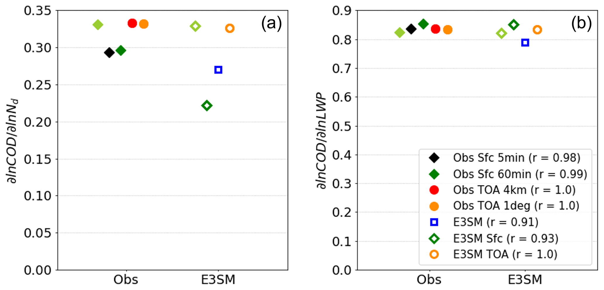
https://acp.copernicus.org/articles/23/13523/2023/acp-23-13523-2023-f11

Figure 11lnCOD as a function of (a) ln N_d and (b) lnLWP for observational and E3SM datasets. Estimates are obtained from ordinary least-squares multiple linear regression with Pearson correlation coefficients shown in the legend. Light-green symbols represent Obs Sfc 60 min and E3SM Sfc datasets with a recomputed N_d that assumes 80 % adiabaticity like the TOA retrievals.

Download

https://acp.copernicus.org/articles/23/13523/2023/acp-23-13523-2023-f12

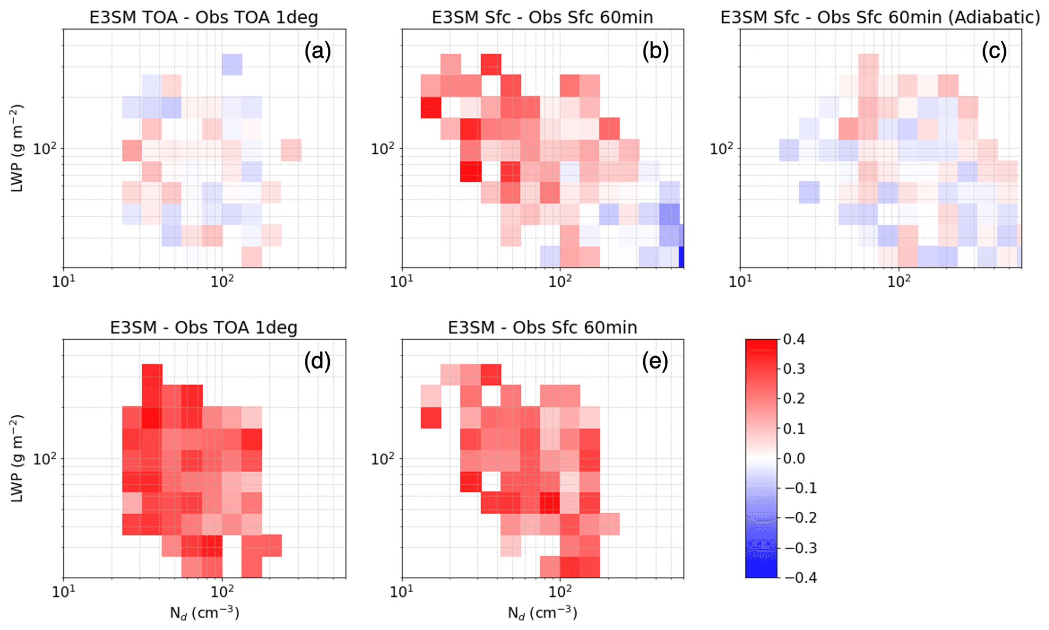
Figure 12Median absolute lnCOD differences between (a) E3SM TOA and Obs TOA 1^∘, (b) E3SM Sfc and Obs Sfc 60 min, and (c) E3SM Sfc and Obs Sfc 60 min using N_d retrievals that assume 80 % adiabaticity, (d) E3SM and Obs Sfc 60 min, and (e) E3SM and Obs TOA 1^∘ as functions of N_d and LWP.

Download

https://acp.copernicus.org/articles/23/13523/2023/acp-23-13523-2023-f13

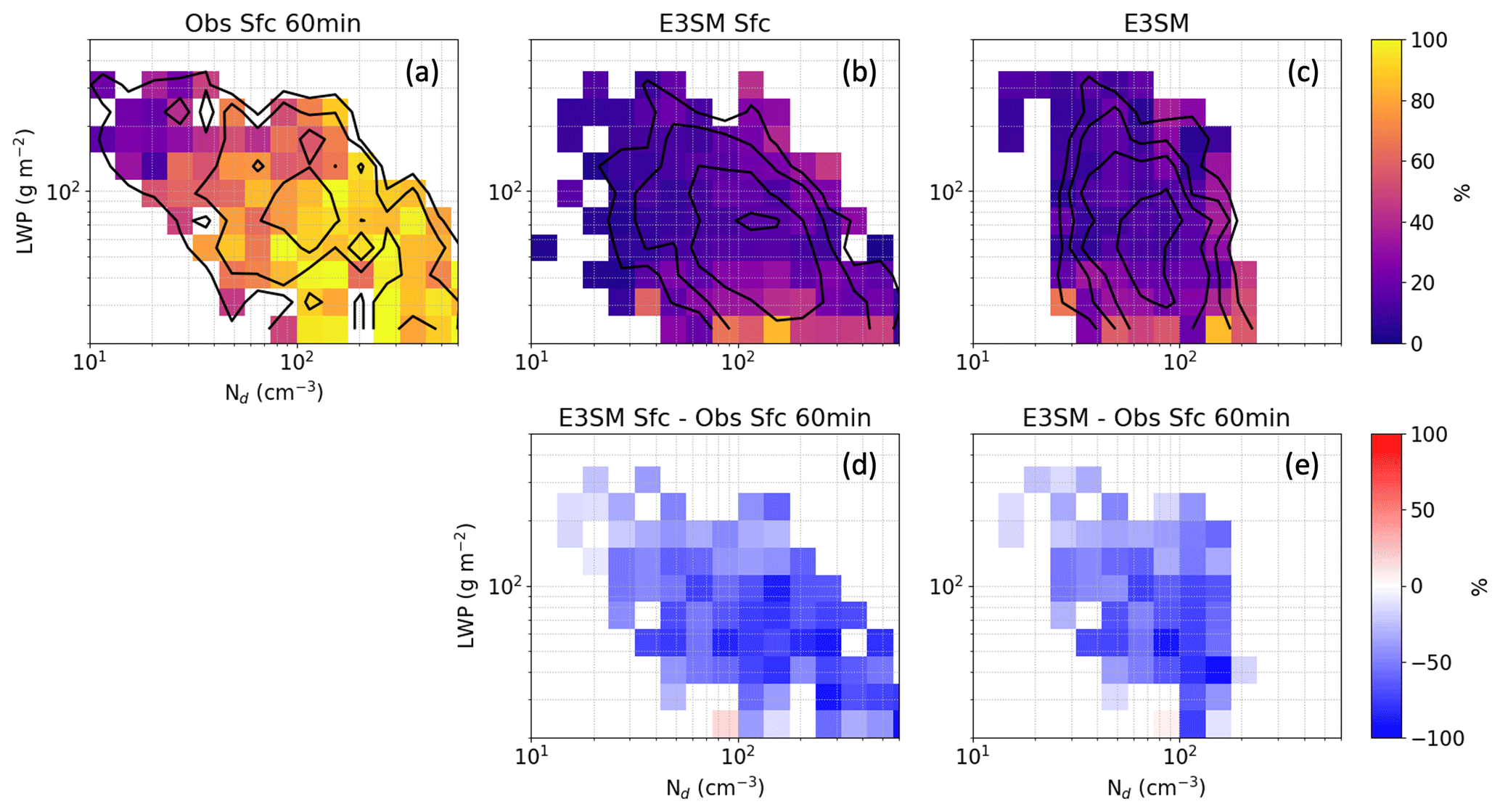
Figure 13Median cloud adiabaticity as a function of LWP and N_d for (a) Obs Sfc 60 min, (b) E3SM Sfc, and (c) E3SM. (d) Absolute differences between E3SM Sfc and Obs Sfc 60 min. (e) Absolute differences between E3SM and Obs Sfc 60 min. Black contours indicate sample size thresholds of 0.4 %, 0.8 %, 1.6 %, and 3.2 %.

Download

https://acp.copernicus.org/articles/23/13523/2023/acp-23-13523-2023-f14

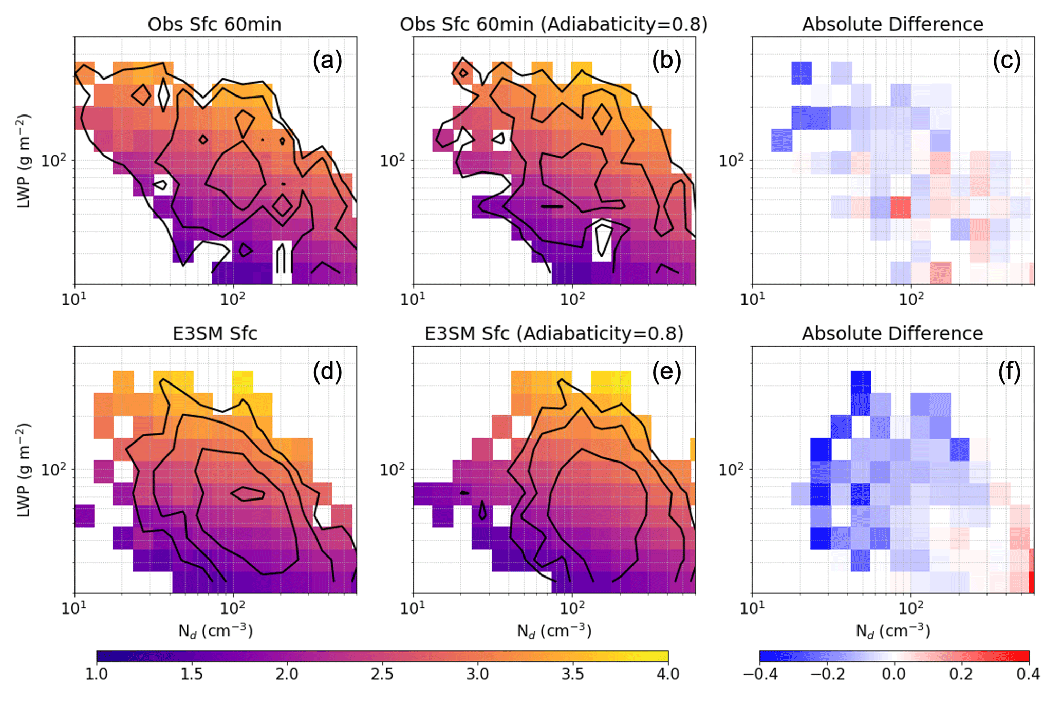
Figure 14Median lnCOD as a function of LWP and N_d for (a) Obs Sfc 60 min, (b) Obs Sfc 60 min using N_d derived assuming 80 % adiabaticity, (c) Obs Sfc 60 min (80 % adiabaticity) minus Obs Sfc 60 min, (d) E3SM Sfc, (e) E3SM Sfc assuming 80 % adiabaticity, and (f) E3SM Sfc (80 % adiabaticity) minus E3SM Sfc. Black contours indicate sample size thresholds of 0.4 %, 0.8 %, 1.6 %, and 3.2 %.

Download

Though simulated and observed values of $\frac{\partial \ln COD}{\partial \ln N_{d}}$ agree once cloud adiabaticity effects on N_d retrievals are removed, lnCOD is always greater than observed for the E3SM direct model output (Fig. 12d and e). This is potentially the result of lower R_eff values in E3SMv1 than observed for given LWP and N_d values (Fig. 15c and d; R_eff values for each dataset are shown in Fig. S7). While R_eff is also systematically lower for given LWP and N_d values in TOA retrievals (Fig. 15a), this does not lead to COD differences as a function of LWP and N_d in the TOA datasets because the exact same N_d calculation is used for Obs TOA and E3SM TOA with sole dependence on LWP, COD, and the constant k parameter that relates droplet volume mean radius to R_eff. The same applies for surface retrievals (Fig. 15b), but non-systematic differences are created by differing adiabaticity values and surface-retrieved R_eff that is sensitive to the entire cloud layer, whereas E3SM Sfc R_eff reflects near-cloud-top values obtained from COSP. That E3SM's R_eff is lower in direct model output than retrievals means that the parameterized size distribution differs from that assumed in observations. Although it is possible that remote-sensing-retrieved R_eff is high biased, recent studies show limited satellite retrieval biases when compared with in situ measurements (Witte et al., 2018; Kang et al., 2021). In addition, aircraft in situ measurements from the ACE-ENA campaign (Wang et al., 2022) support remotely sensed R_eff values being greater in observations than E3SMv1 with corresponding lower N_d values (Wu et al., 2020a). These results provide further support that the simulated SZA–N_d correlation caused by seasonality and the simulated cloud adiabaticity that differs from observations mute the effect of N_d on A in E3SMv1, while smaller R_eff in E3SMv1 than observed amplifies A for a given N_d.

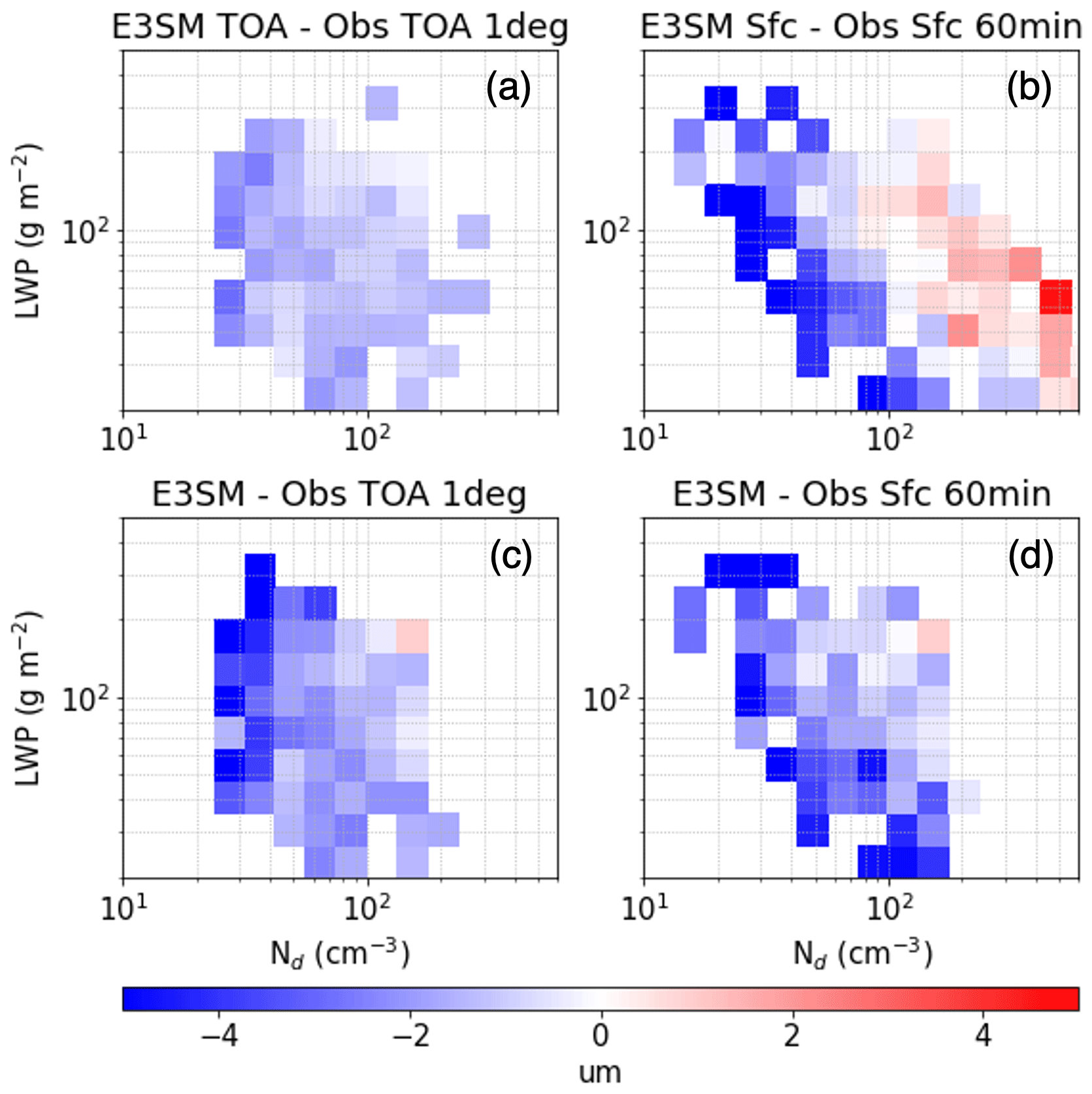
https://acp.copernicus.org/articles/23/13523/2023/acp-23-13523-2023-f15

Figure 15Median absolute R_eff differences between (a) E3SM TOA and Obs TOA 1^∘, (b) E3SM Sfc and Obs Sfc 60 min, (c) E3SM and Obs TOA 1^∘, and (d) E3SM and Obs Sfc 60 min as functions of N_d and LWP.

Download

4.1.3 Aerosol activation into cloud droplets

Twomey effect differences between E3SMv1 and observations also depend on the response of N_d to CCN ( $\frac{d \ln N_{d}}{d \ln CCN}$ ). This term is expected to strongly depend on aerosol activation, though with modulation by N_d sinks such as evaporation and precipitation. It is only evaluated for situations in which clouds are more likely to be coupled with the surface where CCN measurements are made. Although Jones et al. (2011) use a threshold of 0.5 ^∘C for the difference in cloud-base and near-surface potential temperature, we increase this to 2 ^∘C to retain more samples and to account for uncertainty in potential temperature measurements obtained from interpolated soundings that are often separated by 12 h.

Figure 16 shows N_d as a function of surface 0.2 % CCN for all datasets, and correlation coefficients from Theil–Sen robust linear regression are provided in Fig. 17. The sensitivity of N_d to CCN is greater for E3SM direct output than any other dataset. The sensitivity is reduced for E3SM TOA but remains greater than Obs TOA datasets, and it is reduced further for E3SM Sfc, which aligns well with Obs Sfc datasets. The fit is weaker in observations than E3SMv1 as shown by the spread of N_d values for a given CCN value (Fig. 16) and the correlation coefficients in Fig. 17 (0.29–0.54 for observations vs. 0.39–0.85 for E3SMv1 datasets). A substantial portion of this spread is a result of errors in TOA- and surface-retrieved N_d values. This is shown by the greater spread in the COSP- and surface-simulated E3SMv1 N_d relationships compared to the direct N_d relationship, quantified by differences in E3SMv1 correlation coefficients – 0.85 (direct) vs. 0.65 (satellite) and 0.39 (surface) – compared to observational coefficients – 0.46–0.54 (TOA) and 0.29–0.30 (surface). Why do surface-retrieved $\frac{d \ln N_{d}}{d \ln CCN}$ values agree between E3SMv1 and observations while TOA values do not? As for $\frac{\partial \ln COD}{\partial \ln N_{d}}$ discrepancies, this contrast is caused by variable cloud adiabaticity in surface retrievals and constant 80 % adiabaticity in TOA retrievals. When surface-retrieved N_d is recomputed assuming 80 % adiabaticity, E3SMv1's N_d sensitivity to CCN substantially increases, but the observed sensitivity does not (dark-green to light-green symbols in Fig. 17). Thus, once the effect of cloud adiabaticity differences between E3SMv1 and observations on N_d is removed, it becomes clear that the sensitivity of N_d to CCN is too high in E3SMv1. Aircraft-observed N_d vs. CCN concentration during ACE-ENA also supports a conclusion of greater sensitivity in E3SMv1 (Tang et al., 2023). This explains why surface-retrieved N_d values agree between E3SM Sfc and Obs Sfc but are greater for E3SM TOA than Obs TOA. Lower adiabaticities in E3SMv1 than observed have the effect of lowering N_d further from its adiabatic value, but when that effect is removed, it becomes clear that E3SMv1 has higher N_d values than observed despite reasonable CCN values because of a greater sensitivity of N_d to CCN.

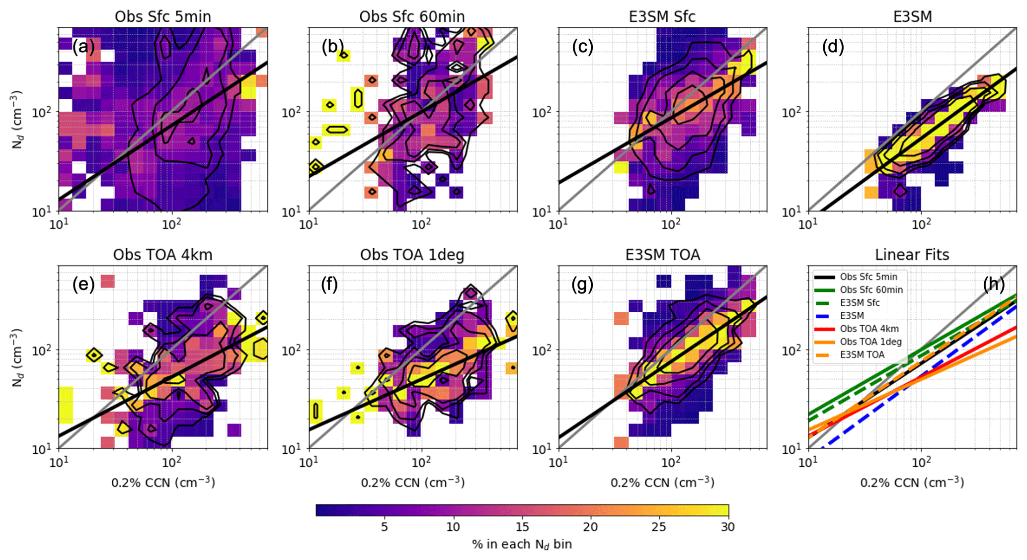
https://acp.copernicus.org/articles/23/13523/2023/acp-23-13523-2023-f16

Figure 16Joint distributions of N_d and 0.2 % CCN number concentration normalized by CCN bin for (a) Obs Sfc 5 min, (b) Obs Sfc 60 min, (c) E3SM Sfc, (d) E3SM, (e) Obs TOA 4 km, (f) Obs TOA 1^∘, and (g) E3SM TOA. Thin black contours indicate sample size thresholds of 0.4 %, 0.8 %, 1.6 %, and 3.2 %. Theil–Sen linear fits are overplotted as a thick solid black with the 1:1 line in gray. Linear fits for each dataset are plotted over one another in (h).

Download

https://acp.copernicus.org/articles/23/13523/2023/acp-23-13523-2023-f17

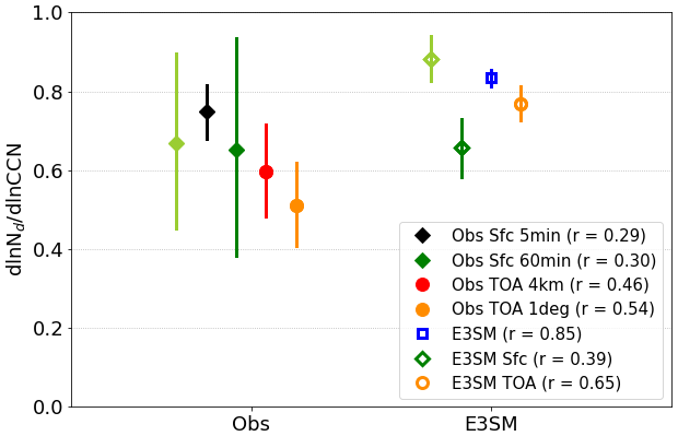
Figure 17ln N_d as a function of lnCCN for observational and E3SM datasets. Estimates are obtained from Theil–Sen robust linear regression with 95 % confidence intervals. Pearson correlation coefficients are shown in the legend. Light-green symbols represent Obs Sfc 60 min and E3SM Sfc datasets with a recomputed N_d that assumes 80 % adiabaticity like the TOA retrievals.

Download

These comparisons suggest that aerosol activation in E3SMv1 is potentially too high. This is consistent with the findings of Ghan et al. (2011) for the Abdul-Razzak–Ghan (ARG) scheme (Abdul-Razzak and Ghan, 2000) used in E3SM. Gong et al. (2023) also find that the ARG scheme coupled with the Cloud Layers Unified by Binormals (Golaz et al., 2002; Larson and Golaz, 2005) and the four-mode Modal Aerosol Module (Liu et al., 2016) in the Community Earth System Model version 2.1 with the Community Atmosphere Model version 6 (Danabasoglu et al., 2020) produces greater cloud supersaturations than retrieved from observations at ENA. With a similar setup in E3SMv1, this could also be influencing the $\frac{d \ln N_{d}}{d \ln CCN}$ differences shown here. However, it is also possible that unrealistic N_d sinks including precipitation and evaporation contribute to $\frac{d \ln N_{d}}{d \ln CCN}$ being greater in E3SMv1 than observed, and more investigation into these processes is required.

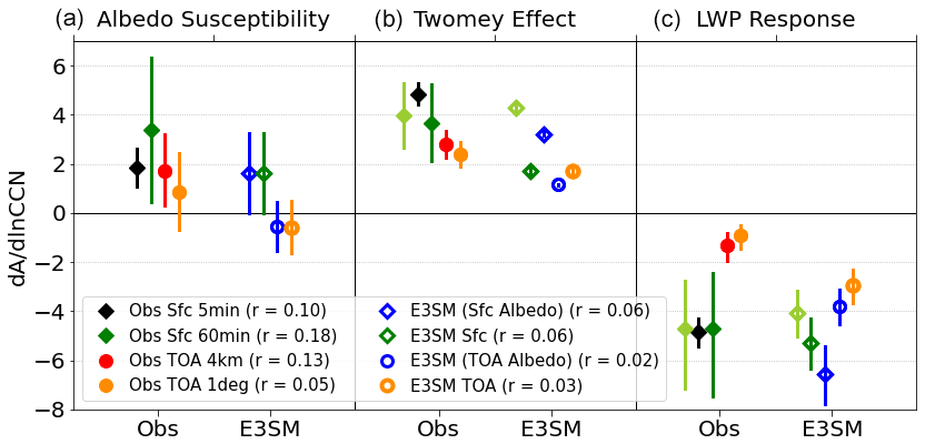
https://acp.copernicus.org/articles/23/13523/2023/acp-23-13523-2023-f18

Figure 18(a) Cloud albedo susceptibility to CCN concentration with (b) the Twomey effect $(\frac{\partial A}{\partial \ln N_{d}} \frac{d \ln N_{d}}{d \ln CCN})$ and (c) LWP response $(\frac{\partial A}{\partial \ln LWP} \frac{d \ln LWP}{d \ln N_{d}} \frac{d \ln N_{d}}{d \ln CCN})$ terms for observational and E3SM datasets with 95 % confidence intervals. Pearson correlation (r) coefficients for albedo regressed on lnCCN are shown in the legend. Note that confidence intervals and r values can seem inconsistent because of differing sample sizes between datasets (see last column in Table 2). Light-green symbols represent Obs Sfc 60 min and E3SM Sfc datasets with a recomputed N_d that assumes 80 % adiabaticity like the TOA retrievals.

Download

E3SMv1–observation $\frac{d \ln N_{d}}{d \ln CCN}$ differences offset $\frac{\partial A}{\partial \ln N_{d}}$ differences for surface retrievals, producing Twomey effect $(\frac{\partial A}{\partial \ln N_{d}} \frac{d \ln N_{d}}{d \ln CCN})$ and albedo susceptibility estimates that are similar (Fig. 18). For TOA estimates, $\frac{\partial A}{\partial \ln N_{d}}$ differences are too great to overcome, leading to a weaker than observed Twomey effect and albedo susceptibility best estimate that is negative (Fig. 18). As discussed in Sect. 4.1.2, this is caused by the negative SZA–N_d correlation in E3SM that is not observed and suppresses $\frac{\partial A}{\partial \ln N_{d}}$ relative to observations. Removing SZA–N_d correlation effects by instead examining COD susceptibility shows in fact that the Twomey effect $(\frac{\partial \ln COD}{\partial \ln N_{d}} \frac{d \ln N_{d}}{d \ln CCN})$ is greater in E3SMv1 than observed, though this is only true for surface retrievals once model–observation cloud adiabaticity differences are removed. Removing adiabaticity effects gives Twomey effects that are about 30 %–40 % greater in E3SMv1 than observed, while lnCOD susceptibility can be up to a factor of 2 greater depending on dataset (Fig. 19).

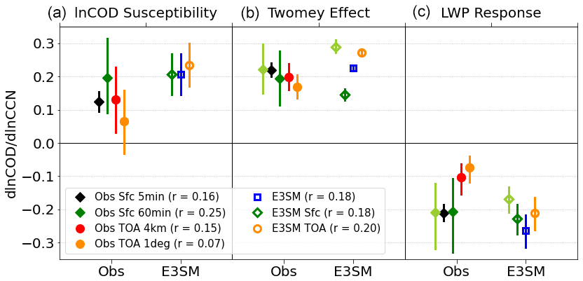
https://acp.copernicus.org/articles/23/13523/2023/acp-23-13523-2023-f19

Figure 19(a) lnCOD susceptibility to CCN concentration with (b) Twomey effect $(\frac{\partial \ln COD}{\partial \ln N_{d}} \frac{d \ln N_{d}}{d \ln CCN})$ and (c) LWP response $(\frac{\partial \ln COD}{\partial \ln LWP} \frac{d \ln LWP}{d \ln N_{d}} \frac{d \ln N_{d}}{d \ln CCN})$ terms for observational and E3SM datasets with 95 % confidence intervals. Pearson correlation (r) coefficients for lnCOD regressed on lnCCN are shown in the legend. Light-green symbols represent Obs Sfc 60 min and E3SM Sfc datasets with a recomputed N_d that assumes 80 % adiabaticity like the TOA retrievals.

Download

4.2 LWP susceptibility comparison

Since only overcast cloud conditions are considered, the second aerosol indirect effect is confined to the LWP susceptibility to N_d $(\frac{d \ln LWP}{d \ln N_{d}})$ , which can accentuate or mute the Twomey effect. Figure 20 shows N_d-bin-normalized joint distributions N_d and LWP for the various datasets analyzed. Like the Twomey effect, the quantified LWP responses depend on the datasets considered since LWP and N_d values shift depending on how they are retrieved. Somewhat poor linear fits are readily apparent, as highlighted by low correlation coefficients (0.21–0.58) in Fig. 21. E3SM susceptibilities range from −0.3 to −0.4, which is similar to those in surface observations, while TOA observations have weaker susceptibilities around −0.2. Removing cloud adiabaticity effects in surface retrievals results in a weaker LWP susceptibility in E3SM than observations, while the opposite is true for TOA retrievals. Thus, there is no consensus among comparisons, and all that can be said is that E3SMv1 has similar values to observed, which differs from most global climate models (GCMs) that produce a positive LWP susceptibility (Quaas et al., 2009; Gryspeerdt et al., 2020).

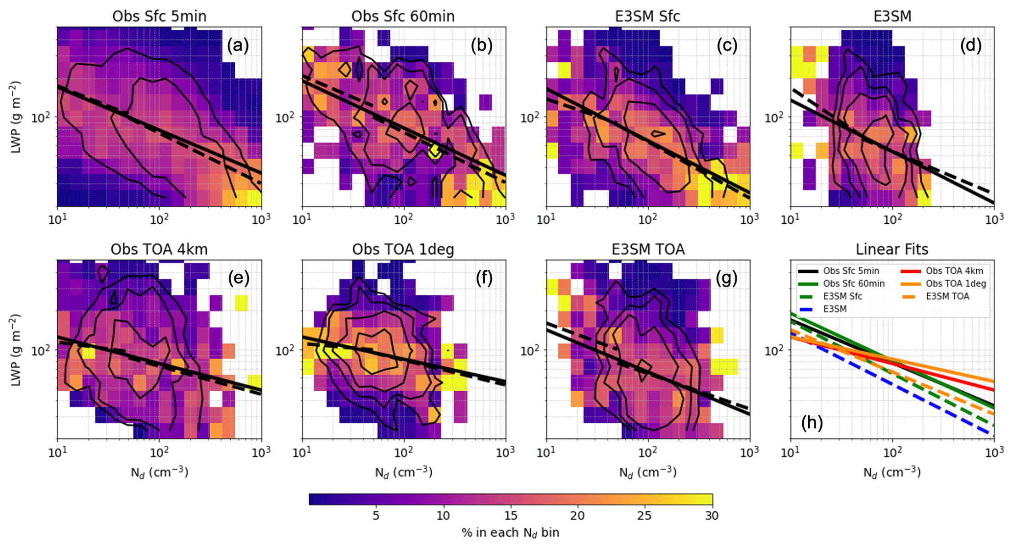
https://acp.copernicus.org/articles/23/13523/2023/acp-23-13523-2023-f20

Figure 20Joint distributions of LWP and N_d normalized by N_d bin for (a) Obs Sfc 5 min, (b) Obs Sfc 60 min, (c) E3SM Sfc, (d) E3SM, (e) Obs TOA 4 km, (f) Obs TOA 1^∘, and (g) E3SM TOA. Thin black contours indicate sample size thresholds of 0.4 %, 0.8 %, 1.6 %, and 3.2 %. Single Theil–Sen linear fits are overplotted in thick solid black, and piecewise fits are overplotted in thick dashed black. Linear fits for each dataset are plotted over one another in (h).

Download

https://acp.copernicus.org/articles/23/13523/2023/acp-23-13523-2023-f21

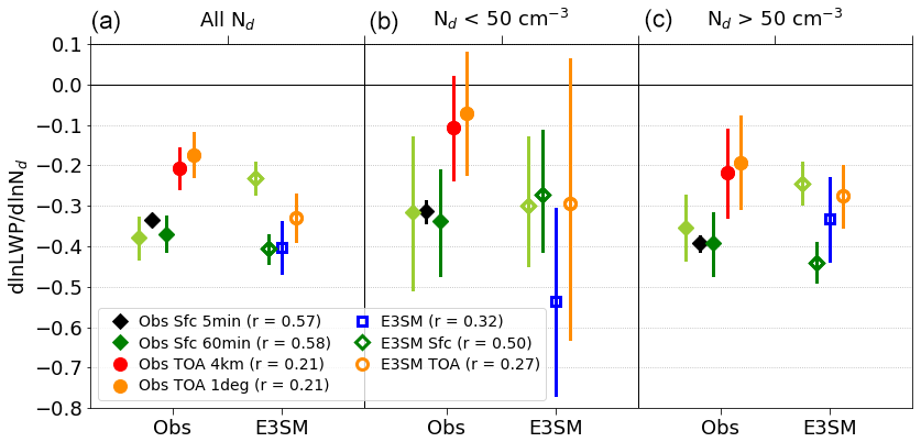
Figure 21lnLWP as a function of ln N_d for (a) all N_d values, (b) N_d<50 cm⁻³, and (c) N_d>50 cm⁻³ for observational and E3SM datasets. Estimates and 95 % confidence intervals are obtained from Theil–Sen robust linear regressions with Pearson correlation coefficients shown in the legend. Light-green symbols represent Obs Sfc 60 min and E3SM Sfc datasets with a recomputed N_d that assumes 80 % adiabaticity like the TOA retrievals.

Download

Previous satellite retrieval and LES studies discussed in the Introduction have highlighted an inverted V response of LWP to N_d, which has been hypothesized to be caused by drizzle suppression at relatively low N_d values increasing LWP but with entrainment-driven evaporation mechanisms reducing LWP for relatively high N_d values in non-drizzling clouds. To assess whether LWP responses to N_d change as N_d increases, linear fits are applied for two different ranges of N_d shown as dashed black lines in Fig. 20a–g and quantified in Fig. 21. Observational datasets become more negative as N_d increases, in agreement with past satellite retrieval studies. However, the opposite trend exists in E3SMv1 direct output and TOA datasets where LWP responses become less negative as N_d increases, with the caveat that uncertainty is high for N_d<50 cm⁻³ due to limited sampling that is possibly associated with constraining analyses to overcast conditions. For surface retrievals, E3SM's LWP susceptibility becomes more negative with increasing N_d like observed, but once cloud adiabaticity is held constant, the opposite occurs, in disagreement with observations. Thus, the change in E3SM's LWP susceptibility with increasing N_d is generally opposite to the expectation from proposed physical mechanisms in past observational and LES studies, indicating possibly different mechanisms that cause its overall negative sign in observations.

4.2.1 Potential physical mechanisms affecting model–observation comparisons

Are negative LWP susceptibilities caused by physical processes, and if so, are they the same in observations and E3SMv1? If clouds are responding to the entrainment–evaporation mechanism, one might expect the LWP susceptibility to change with the inversion strength and above-inversion RH. To assess this, the median LWP susceptibility is plotted in joint EIS–700 hPa RH bins in Fig. 22. No clear dependencies on EIS or RH arise in surface observations (Fig. 22a), while the LWP response becomes less negative as RH increases in TOA observations (Fig. 22c), consistent with more widespread satellite measurements of marine warm clouds in Chen et al. (2014). However, the simulated LWP response to N_d becomes more negative as RH increases for a given EIS (Fig. 22b, d, and e), which indicates that entrainment-driven evaporation is likely not a major control on the negative LWP response in E3SMv1.

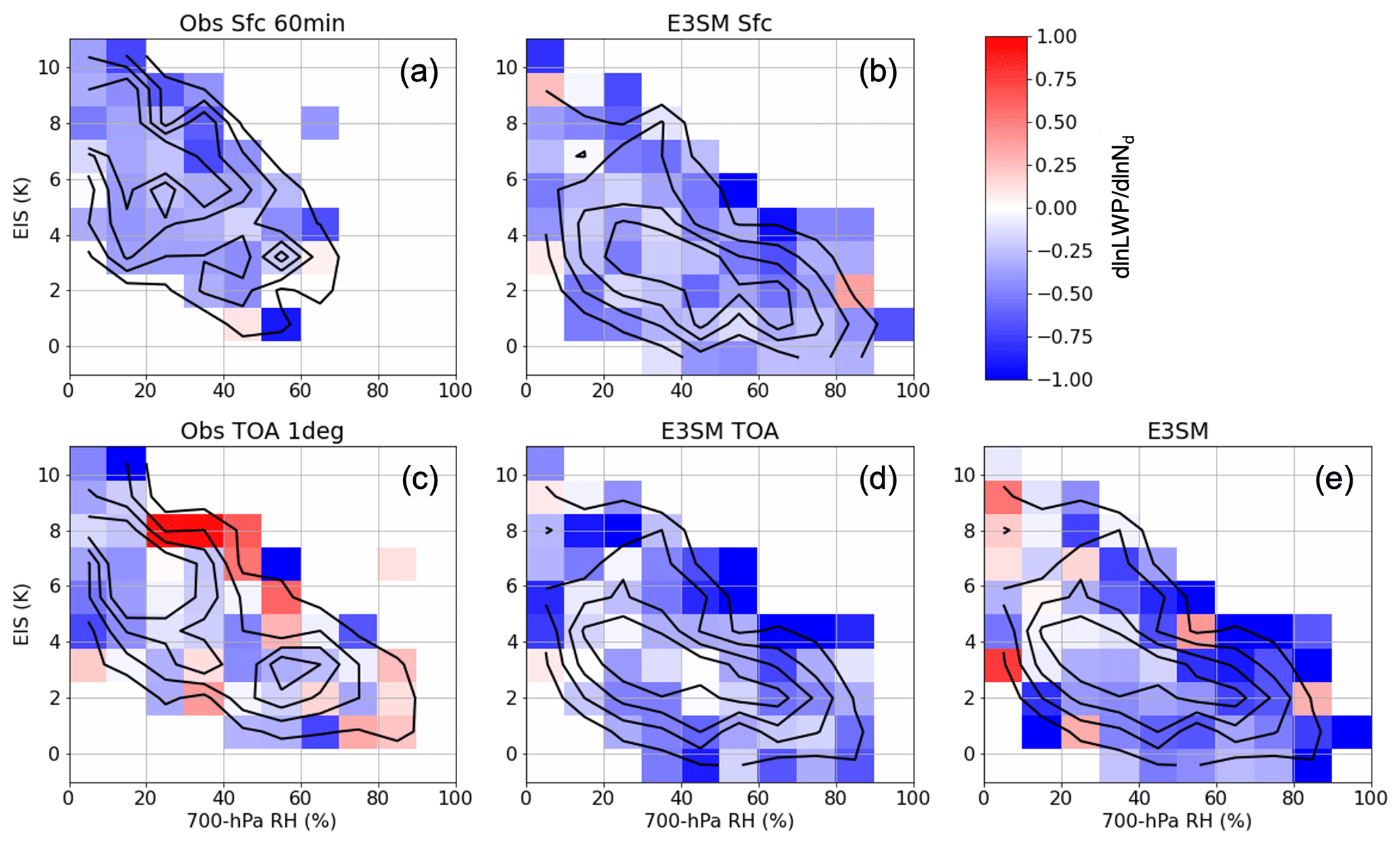
https://acp.copernicus.org/articles/23/13523/2023/acp-23-13523-2023-f22

Figure 22Median LWP response $(\frac{d \ln LWP}{d \ln N_{d}})$ as a function of EIS and 700 hPa RH for (a) Obs Sfc 60 min, (b) E3SM Sfc, (c) Obs TOA 1^∘, (d) E3SM TOA, and (e) E3SM. Black contours indicate sample size thresholds of 0.4 %, 0.8 %, 1.6 %, and 3.2 %.

Download

However, it is apparent from the sample size contours in Fig. 22 that E3SM has fewer occurrences of strong inversions (high EIS) with low 700 hPa RH conditions than observed, consistent with Fig. 5. For a given LWP and N_d value, E3SMv1 can have substantially deeper clouds than observed, often by a couple hundred meters (Fig. S8), and weaker inversions in E3SMv1 are present for all LWP–N_d combinations (Figs. S9 and S10). While E3SM direct model output and surface retrievals have inversions that strengthen as N_d increases with clouds that become shallower, the EIS gradient is notably absent in TOA datasets and the cloud depth dependence on N_d changes sign. This is likely associated with the lack of variable cloud adiabaticity in TOA datasets and suggests caution when using such datasets alone to infer physical processes and evaluate model output. Past studies have shown that weaker stability with boundary layer and cloud deepening causes the LWP susceptibility to become more negative (e.g., Possner et al., 2020; J. Zhang et al., 2022). Thus, one might expect a more negative LWP susceptibility in E3SMv1 than observed if it were properly representing processes controlling the LWP response to N_d, but this is not the case, again suggesting that there are other causes for the negative simulated sign.

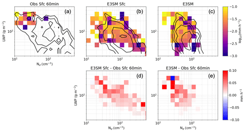
https://acp.copernicus.org/articles/23/13523/2023/acp-23-13523-2023-f23

Figure 23Median surface hourly rain rate as a function of LWP and N_d for (a) Obs Sfc 60 min disdrometer retrievals, (b) E3SM Sfc, and (c) E3SM. (d) Absolute differences between E3SM Sfc and Obs Sfc 60 min. (e) Absolute differences between E3SM and Obs Sfc 60 min. Only rain rates exceeding 0.001 mm h⁻¹ are included in statistics due to observational sensitivity limitations. Black contours indicate sample size thresholds of 0.4 %, 0.8 %, 1.6 %, and 3.2 %.

Download

Another factor affecting LWP susceptibility is cloud adiabaticity (dark- vs. light-green symbols in Fig. 21). In observations, clouds become more adiabatic as N_d increases, potentially due to drizzle suppression (Fig. 13). However, clouds only become slightly more adiabatic as N_d increases in E3SMv1 (Fig. 13). Median hourly surface rain rates as a function of LWP and N_d are shown in Fig. 23 with rain rates less than 0.001 mm h⁻¹ removed due to limited observational sensitivity. Observed clouds with less than 100 g m⁻² LWP or greater than 50 cm⁻³ N_d usually do not have rain reaching the surface, but this is common in E3SMv1 where the sensitivity of surface rain rate to N_d and LWP is muted. The hourly surface rain rate exceeds 0.001 mm h⁻¹ 62 % of the time in E3SMv1 compared to 15 %–18 % in disdrometer and optical rain gauge observations, while rates exceed 0.01 mm h⁻¹ nearly half the time in E3SMv1 as compared to ∼10 % in observations (Table S1 in the Supplement). Total surface rainfall accumulation is also nearly 3 times greater in E3SMv1 as evidenced by average rain rates inclusive of all times in Table S1. Precipitation that is too frequent and light is a well-known problem in GCMs (Stephens et al., 2010; Song et al., 2018) including E3SM (Ma et al., 2022) in which Zheng et al. (2020) noted biases associated with the long microphysics time step and precipitation fraction parameterization. For the single-layer, overcast liquid clouds at ENA assessed here, 84 % of the surface rainfall is produced in the Z–M convection parameterization (Table S1), while the frequency of stratiform drizzle is closer to observed. Figure S11 shows that surface hourly rain rates compare much more favorably when only stratiform rain rates for E3SM and E3SM Sfc are considered, indicating that the Z–M parameterization is a primary driver of the drizzle frequency and amount biases. This is partly caused by deeper clouds in E3SM that more heavily precipitate (Fig. S12), likely a result of weaker inversions in E3SM. However, even for given cloud depth and N_d values, clouds precipitate more heavily (Fig. S12) and are less adiabatic (Fig. S13) than observed. It is probable that the excessive convective drizzle in E3SMv1 contributes to much fewer adiabatic clouds than observed, a difference that increases as N_d increases when observed drizzle ceases but E3SMv1 clouds continue to drizzle with only slightly lower rates (Figs. 13, 23, S12, and S13). It is possible that this muted sensitivity of rain rate and adiabaticity to N_d contributes to the negative relationship of LWP with N_d. Cadeddu et al. (2023) also find that entrainment could be a primary controlling factor of cloud adiabaticity at ENA. How much entrainment affects simulated adiabaticity is not clear, but it is possible that dominant mechanisms controlling adiabaticity and its effects on LWP and N_d differ between E3SMv1 and the real world. More research is needed to better understand how rain rate, entrainment, LWP, and N_d interact to affect albedo susceptibility in both models and the real world.

A final important consideration for interpreting LWP susceptibility quantification is that the LWP–N_d joint distribution is likely not entirely due to N_d effects on LWP. Confounding factors such as meteorology or mesoscale cloud structures may combine with microphysical processes to create overall negative LWP–N_d relationships. Indeed, present-day minus pre-industrial E3SMv1 simulations produce a positive rather than negative LWP susceptibility (Christensen et al., 2023). Albedo and COD susceptibilities are also generally slightly less than Twomey effects $(\frac{\partial A}{\partial \ln N_{d}} \frac{d \ln N_{d}}{d \ln CCN}$ , $\frac{\partial \ln COD}{\partial \ln N_{d}} \frac{d \ln N_{d}}{d \ln CCN})$ despite LWP response $(\frac{\partial A}{\partial \ln LWP} \frac{d \ln LWP}{d \ln N_{d}} \frac{d \ln N_{d}}{d \ln CCN}$ , $\frac{\partial \ln COD}{\partial \ln LWP} \frac{d \ln LWP}{d \ln N_{d}} \frac{d \ln N_{d}}{d \ln CCN})$ estimates that are large enough to completely cancel the Twomey effects (Figs. 18 and 19). This suggests that spread in the $\frac{d \ln LWP}{d \ln N_{d}}$ and $\frac{d \ln N_{d}}{d \ln CCN}$ relationships and unaccounted-for covariations between lnLWP and lnCCN partly counteract the estimated LWP response. Thus, further research is needed to develop methods for sufficiently evaluating cloud adjustments in GCMs using present-day observations.

5 Conclusions

Surface-based and satellite observations collected at the ARM ENA site in the Azores over 5 years were used to evaluate factors controlling single-layer liquid cloud albedo susceptibility for overcast cloud conditions in E3SMv1. While a single geographical location such as the ENA site is not representative of all environments and cloud types, its relatively comprehensive measurements and retrievals, including CCN number concentration, atmospheric stability and humidity, and radiative fluxes, as well as cloud LWP, N_d, rain rate, and cloud adiabaticity in a marine environment with frequent single-layer liquid clouds susceptible to aerosol influences, allow for detailed model evaluation targeting specific processes. This methodology provides valuable context for more traditional model evaluation via longer-term global metrics. Surface retrievals with 5 and 60 min resolutions, geostationary satellite retrievals with 4 km and 1^∘ resolutions, and 1^∘ resolution E3SMv1 datasets using different N_d and LWP retrievals from raw model output, COSP satellite simulator output, and surface variables are all analyzed to assess the robustness of model–observation comparisons.

Simulated cloud albedo values are greater for given LWP and N_d values due to R_eff being smaller than retrieved in observations. However, cloud albedo sensitivities to N_d and LWP are well simulated by E3SMv1 after accounting for a simulated SZA–N_d correlation caused by seasonality that is not observed by analyzing COD susceptibility and after accounting for differences in observed and simulated cloud adiabaticity. Both effects mute the simulated sensitivity of cloud albedo to N_d. E3SMv1 adiabaticities are much lower than observed and the common 80 % assumed in satellite retrievals, and adiabaticities affect the sensitivity of cloud albedo to ln N_d by altering the width of the ln N_d distribution. LWP is also less than observed, while N_d is greater than observed if cloud adiabaticity differences between E3SMv1 and observations are removed, despite a similar overall distribution of surface CCN concentration to observed. Because of logarithmic sensitivities, this means that linear perturbations in N_d will result in a lower Twomey effect in E3SMv1 compared to observations at ENA, though perturbations in LWP could potentially result in a greater effect.

Greater N_d values in E3SMv1 may result from excessive activation of CCN. This drives a Twomey effect that is too large by 30 %–40 % when using TOA- and surface-retrieved N_d values. However, this difference again only emerges after controlling for SZA and cloud adiabaticity. LWP decreases as N_d increases like observed, something that is not produced by most GCMs. However, the LWP susceptibility becomes more negative in E3SMv1 as above-inversion RH increases, a trend that is not observed and is not consistent with drier conditions facilitating more evaporation. In addition, the simulated LWP susceptibility does not become more negative as N_d increases like observed. Thus, it is unlikely that an entrainment-driven evaporation mechanism is operating in E3SMv1. E3SMv1 also has weaker inversions and deeper clouds than observed, which partly contributes to excessive convectively driven drizzle that is a common bias in GCMs (Stephens et al., 2010), though a substantial bias remains after controlling for cloud depth. There is also little decrease in drizzle rate and little increase in cloud adiabaticity as N_d increases for a given LWP or cloud depth in E3SMv1, which is in stark contrast to observations. Because of these major differences in observed and simulated cloud properties, the causes of the similar negative LWP susceptibility in E3SMv1 and observations likely differ. The negative LWP responses also only slightly decrease the overall cloud albedo susceptibilities, especially for E3SMv1, indicating that there are confounding effects that render a statistical correlation between LWP and N_d insufficient for assessing N_d impacts on LWP.

Because E3SMv1 has a greater Twomey effect than observed and because adjustments lower the COD susceptibility more in observations than E3SMv1, simulated COD susceptibility values are about double those observed after controlling for cloud adiabaticity differences, which is consistent with overly negative ERFaci assessed in previous studies (Golaz et al., 2019; Rasch et al., 2019; Wang et al., 2020; Ma et al., 2022; K. Zhang et al., 2022). This also indicates that greater $\frac{d \ln N_{d}}{d \ln CCN}$ values in E3SMv1, as modulated by aerosol activation, N_d evaporation, and precipitation, along with less muting by adjustments, are the primary drivers of greater radiative susceptibilities to aerosols in E3SMv1.

Differences between E3SMv1 and observations often exceed the observational spreads after critically controlling for cloud adiabaticity model–observation differences, but the spreads are still substantial. Both retrieval scale and simplifying assumptions contribute similar magnitudes of uncertainty in quantifying cloud albedo susceptibility and the Twomey effect, while retrieval assumptions contribute the most uncertainty in quantifying the LWP susceptibility. A major contributor to these discrepancies is the retrieval of N_d. For the most accurate N_d retrieval, it is best to compute N_d at the highest resolution possible and average it to coarser scales (McComiskey and Feingold, 2012; Feingold et al., 2022). However, because E3SM surface and TOA N_d retrievals were performed using E3SMv1 1^∘ output, 1^∘ and 60 min observational N_d retrievals were instead computed using inputs averaged to those scales so that comparisons used consistent methods. This creates differences as a function of data resolution. However, the spreads in Twomey effect and LWP susceptibility estimates from E3SMv1 are of similar magnitude to observational spreads despite being computed at a constant resolution. This occurs because the retrieval assumptions create shifts in the N_d distribution relative to its true shape in direct model output. Retrieval biases are to be expected given assumptions of constant N_d in the cloud layer, drizzle contamination, and scaled adiabatic droplet growth between cloud base and cloud top, but this clearly demonstrates the significant impacts of such assumptions in quantifying aerosol–cloud interactions.

Multiple model–observation comparison approaches like those used in this study coupled with in situ data comparisons provide critical context in the absence of well-quantified sampling and retrieval biases. Comparative analyses used in this study are being implemented into the open-source ESMAC-Diags software package (Tang et al., 2022, 2023) and expanded to additional locations with differing aerosol, cloud, and meteorological conditions such that E3SMv2 and future versions can be assessed in the same manner. However, despite designing this study to have interpretable model–observation comparisons, it does not overcome several key issues that have led to persistent uncertainty of ERFaci through successive generations of climate models. These include the small magnitude of ERFaci relative to the total shortwave cloud radiative effect, its dependency on massive cross-scale atmospheric interactions, an inability to isolate specific model components that contribute to errors, and an inability to estimate such effects with sufficient accuracy in observations (Mülmenstädt and Feingold, 2018). Furthermore, it does not overcome the problem of present-day statistically derived cloud susceptibilities being insufficient to describe susceptibilities based on present-day minus pre-industrial conditions (e.g., Ghan et al., 2016; Christensen et al., 2022). There are also observational complexities that were not considered that could impact conclusions. Namely, possible Graciosa Island effects on clouds (e.g., Ghate et al., 2021; Jeong et al., 2022) were not considered. Drizzle contamination can also bias LWP retrievals (e.g., Cadeddu et al., 2020), which can then impact N_d retrievals using LWP as an input, particularly for relatively high-LWP and low-N_d conditions.

There are several implications of this study's results. First, the diurnal and seasonal cycles of LWP and N_d can modulate cloud albedo susceptibility due to correlations with the SZA, which impacts interpretations of model–observation differences. Second, large uncertainties exist due to N_d retrieval assumptions that limit our ability to accurately quantify factors affecting cloud albedo susceptibility. Continued and expanded integration of complementary in situ, remote sensing, and high-resolution model datasets will aid this effort. Critical to properly predicting albedo susceptibility are improved understanding and quantification of LWP and CF adjustments that respond to poorly simulated small-scale entrainment and precipitation processes operating over days and hundreds of kilometers, processes that are not well represented in GCMs. Of equal importance is improving parameterized activation of aerosol particles into cloud droplets, which is known to be problematic (e.g., Ghan et al., 2011) and can turn realistic simulated radiation responses to N_d perturbations into greatly amplified (as in this study) or muted responses to aerosol perturbations. Recent work shows promise in improving aerosol activation parameterization (e.g., Silva et al., 2021), though relationships between N_d and CCN can also be affected by precipitation scavenging that complicates interpretations of observations. Further studies are also required to critically improve simulated drizzle and entrainment processes that influence quantification of both the Twomey effect and cloud adjustments via impacts on cloud adiabaticity. Lastly, more studies are needed to assess how confounding factors such as erroneous responses to meteorology (e.g., Eastman et al., 2021) contribute to susceptibilities and interpretations of model–observation comparisons.

Code and data availability

Files containing all the observations, E3SM output variables, and necessary E3SM setup files used in this study can be downloaded from https://doi.org/10.5281/zenodo.8436534 (Varble et al., 2023). Python notebooks used to make these files including retrievals of several variables can also be downloaded from the same location. Original DOE ARM datasets at the ENA site used in this research can be downloaded from the links provided in each dataset's citation.

Supplement

The supplement related to this article is available online at: https://doi.org/10.5194/acp-23-13523-2023-supplement.

Author contributions

ACV wrote the paper, performed analyses, and created visualizations. PLM performed E3SMv1 simulations. Research conceptualization, as well as reviewing and editing of the paper, was performed by ACV, PLM, MWC, JM, ST, and JF.

Competing interests

The contact author has declared that none of the authors has any competing interests.

Disclaimer

Publisher's note: Copernicus Publications remains neutral with regard to jurisdictional claims made in the text, published maps, institutional affiliations, or any other geographical representation in this paper. While Copernicus Publications makes every effort to include appropriate place names, the final responsibility lies with the authors.

Acknowledgements

This research used resources from the National Energy Research Scientific Computing Center (NERSC), a US Department of Energy Office of Science User Facility located at Lawrence Berkeley National Laboratory, operated under contract no. DE-AC02-05CH11231 using NERSC awards ALCCERCAP0016315, BER-ERCAP0015329, BER-ERCAP0018473, and BER-ERCAP0020990. We thank the numerous ARM instrument and data mentors for providing data. We also thank Zhibo Zhang and an anonymous reviewer for helpful feedback that improved the quality of this paper. The Pacific Northwest National Laboratory is operated for the US Department of Energy by Battelle Memorial Institute under contract no. DE-AC05-76RL01830.

Financial support

This study was funded by the US Department of Energy, Office of Science, Office of Biological and Environmental Research, Earth System Model Development (ESMD) program via the Enabling Aerosol–cloud interactions at Global convection-permitting scalES (EAGLES) project (project no. 74358).

Review statement

This paper was edited by Matthew Lebsock and reviewed by Zhibo Zhang and one anonymous referee.

References

Abdul-Razzak, H. and Ghan, S. J.: A parameterization of aerosol activation: 2. Multiple aerosol types, J. Geophys. Res., 105, 6837–6844, https://doi.org/10.1029/1999JD901161, 2000.

Ackerman, A. S., Kirkpatrick, M. P., Stevens, D. E., and Toon, O. B.: The impact of humidity above stratiform clouds on indirect aerosol climate forcing, Nature, 432, 1014–1017, https://doi.org/10.1038/nature03174, 2004.

Albrecht, B. A.: Aerosols, Cloud Microphysics, and Fractional Cloudiness, Science, 245, 1227–1230, https://doi.org/10.1126/science.245.4923.1227, 1989.

ARM – Atmospheric Radiation Measurement user facility: Interpolated Sonde (INTERPOLATEDSONDE), 2016-01-01 to 2020-12-31, Eastern North Atlantic (ENA) Graciosa Island, Azores, Portugal (C1), compiled by: Jensen, M., Giangrande, S., Fairless, T., and Zhou, A., ARM Data Center [data set], https://doi.org/10.5439/1095316, 2013a.

ARM – Atmospheric Radiation Measurement user facility: Minnis Cloud Products Using Visst Algorithm (VISSTGRIDM10MINNIS), 2016-01-01 to 2018-02-20, Eastern North Atlantic (ENA) External Data (satellites and others) (X1), ARM Data Center [data set], https://adc.arm.gov/discovery/#/results/datastream::enavisstgridm10minnisX1.c1 (last access: 12 August 2021), 2013b.

ARM – Atmospheric Radiation Measurement user facility: Surface Meteorological Instrumentation (MET), 2016-01-01 to 2020-12-31, Eastern North Atlantic (ENA) Graciosa Island, Azores, Portugal (C1), compiled by: Kyrouac J., and Shi, Y., ARM Data Center [data set], https://doi.org/10.5439/1786358, 2013c.

ARM – Atmospheric Radiation Measurement user facility: Cloud Optical Properties from MFRSR Using Min Algorithm (MFRSRCLDOD1MIN), 2016-01-01 to 2020-12-31, Eastern North Atlantic (ENA) Graciosa Island, Azores, Portugal (C1), compiled by: Zhang, D., ARM Data Center [data set], https://doi.org/10.5439/1027296, 2014a.

ARM – Atmospheric Radiation Measurement user facility: Laser Disdrometer Quantities (LDQUANTS), 2016-01-01 to 2020-12-31, Eastern North Atlantic (ENA) Graciosa Island, Azores, Portugal (C1), compiled by: Hardin, J., Giangrande, S., and Zhou, A., ARM Data Center [data set], https://doi.org/10.5439/1432694, 2014b.

ARM – Atmospheric Radiation Measurement user facility: Minnis Cloud Products Using Visst Algorithm (VISSTPXM10MINNIS), 2016-01-01 to 2018-02-20, Eastern North Atlantic (EN) External Data (satellites and others) (X1), ARM Data Center [data set], https://adc.arm.gov/discovery/#/results/datastream::enavisstpx2dm10minnisX1.c1 (last access: 12 August 2021), 2014c.

ARM – Atmospheric Radiation Measurement user facility: MWR Retrievals with MWRRET Version 2 (MWRRET2TURN), 2016-01-01 to 2020-12-31, Eastern North Atlantic (ENA) Graciosa Island, Azores, Portugal (C1), compiled by: Gaustad, K., ARM Data Center [data set], https://doi.org/10.5439/1566156, 2014d.

ARM – Atmospheric Radiation Measurement user facility: Active Remote Sensing of CLouds (ARSCL) product using Ka-band ARM Zenith Radars (ARSCLKAZRBND1KOLLIAS), 2016-01-01 to 2020-12-31, Eastern North Atlantic (ENA) Graciosa Island, Azores, Portugal (C1), compiled by: Johnson, K., Giangrande, S., and Toto, T., ARM Data Center [data set], https://doi.org/10.5439/1393438, 2015.

ARM – Atmospheric Radiation Measurement user facility: Cloud Condensation Nuclei Particle Counter (AOSCCN1COLAVG), 2016-06-22 to 2020-10-28, Eastern North Atlantic (ENA) Graciosa Island, Azores, Portugal (C1), compiled by: Koontz, A. and Flynn, C., ARM Data Center [data set], https://doi.org/10.5439/1255094, 2016a.

ARM – Atmospheric Radiation Measurement user facility: Cloud Condensation Nuclei Particle Counter (AOSCCN1COLSPECTRA), 2016-06-22 to 2020-10-28, Eastern North Atlantic (ENA) Graciosa Island, Azores, Portugal (C1), compiled by: Uin, J., ARM Data Center [data set], https://doi.org/10.5439/1342134, 2016b.

ARM – Atmospheric Radiation Measurement user facility: Minnis Cloud Products Using Visst Algorithm (VISSTGRIDM11MINNIS), 2018-02-20 to 2020-12-31, Eastern North Atlantic (EN) External Data (satellites and others) (X1), ARM Data Center [data set], https://adc.arm.gov/discovery/#/results/datastream::enavisstgridm11minnisX1.c1 (last access: 12 August 2021), 2018a.

ARM – Atmospheric Radiation Measurement user facility: Minnis Cloud Products Using Visst Algorithm (VISSTPX2DM11MINNIS), 2018-02-20 to 2020-12-31, Eastern North Atlantic (ENA) External Data (satellites and others) (X1), ARM Data Center [data set], https://adc.arm.gov/discovery/#/results/datastream::enavisstpx2dm11minnisX1.c1 (last access: 12 August 2021), 2018b.

Bellouin, N., Quaas, J., Gryspeerdt, E., Kinne, D., Stier, P., Watson-Parris, D., Boucher, O., Carslaw, K. S., Christensen, M., Daniau, A.-L., Dufresne, J.-L., Feingold, G., Fiedler, S., Forster, P., Gettelman, A., Haywood, J. M., Lohmann, U., Malavelle, F., Mauritsen, T., McCoy, D. T., Myhre, G., Mülmenstädt, J., Neubauer, D., Possner, A., Rugenstein, M., Sato, Y., Schulz, M., Schwartz, S. E., Sourdeval, O., Storelvmo, T., Toll, V., Winker, D., and Stevens, B.: Bounding global aerosol radiative forcing of climate change, Rev. Geophys., 58, e2019RG000660, https://doi.org/10.1029/2019RG000660, 2020.

Bennartz, R.: Global assessment of marine boundary layer cloud droplet number concentration from satellite, J. Geophys. Res.-Atmos., 112, D02201, https://doi.org/10.1029/2006JD007547, 2007.

Bodas-Salcedo, A., Webb, M. J., Bony, S., Chepfer, H., Dufresne, J.-L., Klein, S. A., Zhang, Y., Marchand, R., Haynes, J. M., Pincus, R., and John, V. O.: COSP: Satellite simulation software for model assessment, B. Am. Meteorol. Soc., 92, 1023–1043, https://doi.org/10.1175/2011BAMS2856.1, 2011.

Boers, R. and Mitchell, R. M.: Absorption feedback in stratocumulus clouds influence on cloud top albedo, Tellus A, 46, 229–241, https://doi.org/10.1034/j.1600-0870.1994.00001.x, 1994.

Boucher, O., Randall, D., Artaxo, P., Bretherton, C., Feingold, G., Forster, P., Kerminen, V.-M., Kondo, Y., Liao, H., Lohmann, U., Rasch, P., Satheesh, S., Sherwood, S., Stevens, B., and Zhang, X.: Clouds and aerosols, in: Climate change 2013: The physical science basis, Contribution of Working Group I to the Fifth Assessment Report of the Intergovernmental Panel on Climate Change, Chap. 7, edited by: Stocker, T., Qin, D., Plattner, G.-K., Tignor, M., Allen, S., Boschung, J., Nauels, A., Xia, Y., Bex, V., and Midgley, P., Cambridge University Press, Cambridge, UK and New York, NY, USA, 571–658, https://doi.org/10.1017/CBO9781107415324.016, 2013.

Brenguier, J.-L., Burnet, F., and Geoffroy, O.: Cloud optical thickness and liquid water path – does the k coefficient vary with droplet concentration?, Atmos. Chem. Phys., 11, 9771–9786, https://doi.org/10.5194/acp-11-9771-2011, 2011.

Bretherton, C. S., Blossey, P. N., and Uchida, J.: Cloud droplet sedimentation, entrainment efficiency, and subtropical stratocumulus albedo, Geophys. Res. Lett., 34, L03813, https://doi.org/10.1029/2006GL027648, 2007.

Cadeddu, M. P., Liljegren, J. C., and Turner, D. D.: The Atmospheric radiation measurement (ARM) program network of microwave radiometers: instrumentation, data, and retrievals, Atmos. Meas. Tech., 6, 2359–2372, https://doi.org/10.5194/amt-6-2359-2013, 2013.

Cadeddu, M. P., Ghate, V. P., and Mech, M.: Ground-based observations of cloud and drizzle liquid water path in stratocumulus clouds, Atmos. Meas. Tech., 13, 1485–1499, https://doi.org/10.5194/amt-13-1485-2020, 2020.

Cadeddu, M. P., Ghate, V. P., Turner, D. D., and Surleta, T. E.: Boundary layer moisture variability at the Atmospheric Radiation Measurement (ARM) Eastern North Atlantic observatory during marine conditions, Atmos. Chem. Phys., 23, 3453–3470, https://doi.org/10.5194/acp-23-3453-2023, 2023.

Carslaw, K., Lee, L., Reddington, C., Pringle, K. J., Rap, A., Forster, P. M., Mann, G. W., Spracklen, D. V., Woodhouse, M. T., Regayre, L. A., and Pierce, J. R.: Large contribution of natural aerosols to uncertainty in indirect forcing, Nature, 503, 67–71, https://doi.org/10.1038/nature12674, 2013.

Chen, YC., Christensen, M., Stephens, G., and Seinfeld, J. H.: Satellite-based estimate of global aerosol–cloud radiative forcing by marine warm clouds, Nat. Geosci., 7, 643–646, https://doi.org/10.1038/ngeo2214, 2014.

Christensen, M. W., Neubauer, D., Poulsen, C. A., Thomas, G. E., McGarragh, G. R., Povey, A. C., Proud, S. R., and Grainger, R. G.: Unveiling aerosol–cloud interactions – Part 1: Cloud contamination in satellite products enhances the aerosol indirect forcing estimate, Atmos. Chem. Phys., 17, 13151–13164, https://doi.org/10.5194/acp-17-13151-2017, 2017.

Christensen, M. W., Jones, W. K., and Stier, P.: Aerosols Enhance Cloud Lifetime and Brightness along the Stratus-to-Cumulus Transition, P. Natl. Acad. Sci. USA, 117, 17591–17598, https://doi.org/10.1073/pnas.1921231117, 2020.

Christensen, M. W., Gettelman, A., Cermak, J., Dagan, G., Diamond, M., Douglas, A., Feingold, G., Glassmeier, F., Goren, T., Grosvenor, D. P., Gryspeerdt, E., Kahn, R., Li, Z., Ma, P.-L., Malavelle, F., McCoy, I. L., McCoy, D. T., McFarquhar, G., Mülmenstädt, J., Pal, S., Possner, A., Povey, A., Quaas, J., Rosenfeld, D., Schmidt, A., Schrödner, R., Sorooshian, A., Stier, P., Toll, V., Watson-Parris, D., Wood, R., Yang, M., and Yuan, T.: Opportunistic experiments to constrain aerosol effective radiative forcing, Atmos. Chem. Phys., 22, 641–674, https://doi.org/10.5194/acp-22-641-2022, 2022.

Christensen, M. W., Ma, P.-L., Wu, P., Varble, A. C., Mülmenstädt, J., and Fast, J.: Evaluation of aerosol-cloud interactions in E3SSM using a Lagrangian framework, Atmos. Chem. Phys., 23, 2789–2812, https://doi.org/10.5194/acp-23-2789-2023, 2023.

Clothiaux, E. E., Ackerman, T. P., Mace, G. G., Moran, K. P., Marchand, R. T., Miller, M. A., and Martner, B. E.: Objective determination of cloud heights and radar reflectivities using a combination of active remote sensors at the ARM CART sites, J. Appl. Meteorol., 39, 645–665, https://doi.org/10.1175/1520-0450(2000)039<0645:ODOCHA>2.0.CO;2, 2000.

Coakley, J. A., Bernstein, R. L., and Durkee, P. A.: Effect of Ship-Stack Effluents on Cloud Reflectivity, Science, 237, 1020–1022, https://doi.org/10.1126/science.237.4818.1020, 1987.

Danabasoglu, G., Lamarque, J.-F., Bacmeister, J., Bailey, D. A., DuVivier, A. K., Edwards, J., Emmons, L. K., Fasullo, J., Garcia, R., Gettelman, A., Hannay, C., Holland, M. M., Large, W. G., Lauritzen, P. H., Lawrence, D. M., Lenaerts, J. T. M., Lindsay, K., Lipscomb, W. H., Mills, M. J., Neale, R., Oleson, K. W., Otto-Bliesner, B., Phillips, A. S., Sacks, W., Tilmes, S., van Kampenhout, L., Vertenstein, M., Bertini, A., Dennis, J., Deser, C., Fischer, C., Fox-Kemper, B., Kay, J. E., Kinnison, D., Kushner, P. J., Larson, V. E., Long, M. C., Mickelson, S., Moore, J. K., Nienhouse, E., Polvani, L., Rasch, P. J., and Strand, W. G.: The Community Earth System Model Version 2 (CESM2), J. Adv. Model. Earth Syst., 12, e2019MS001916, https://doi.org/10.1029/2019MS001916, 2020.

Dong, X., Xi, B., Kennedy, A., Minnis, P., and Wood, R.: A 19-month record of marine aerosol-cloud-radiation properties derived from DOE ARM Mobile Facility deployment at the Azores. Part I: cloud fraction and single-layered MBL cloud properties, J. Climate, 27, 3665–3682, https://doi.org/10.1175/JCLI-D-13-00553.1, 2014.

Dong, X., Schwantes, A. C., Xi, B., and Wu, P.: Investigation of the marine boundary layer cloud and CCN properties under coupled and decoupled conditions over the Azores, J. Geophys. Res.-Atmos., 120, 6179–6191, https://doi.org/10.1002/2014JD022939, 2015.

Douglas, A. and L'Ecuyer, T.: Quantifying variations in shortwave aerosol–cloud–radiation interactions using local meteorology and cloud state constraints, Atmos. Chem. Phys., 19, 6251–6268, https://doi.org/10.5194/acp-19-6251-2019, 2019.

Douglas, A. and L'Ecuyer, T.: Quantifying cloud adjustments and the radiative forcing due to aerosol–cloud interactions in satellite observations of warm marine clouds, Atmos. Chem. Phys., 20, 6225–6241, https://doi.org/10.5194/acp-20-6225-2020, 2020.

Eastman, R., Wood, R., and Bretherton, C. S.: Time Scales of Clouds and Cloud-Controlling Variables in Subtropical Stratocumulus from a Lagrangian Perspective, J. Atmos. Sci., 73, 3079–3091, https://doi.org/10.1175/JAS-D-16-0050.1, 2016.

Eastman, R., Terai, C. R., Grosvenor, D. P., and Wood, R.: Evaluating the Lagrangian Evolution of Subtropical Low Clouds in GCMs Using Observations: Mean Evolution, Time Scales, and Responses to Predictors, J. Atmos. Sci., 78, 353–372, https://doi.org/10.1175/JAS-D-20-0178.1, 2021.

Eyring, V., Bony, S., Meehl, G. A., Senior, C. A., Stevens, B., Stouffer, R. J., and Taylor, K. E.: Overview of the Coupled Model Intercomparison Project Phase 6 (CMIP6) experimental design and organization, Geosci. Model Dev., 9, 1937–1958, https://doi.org/10.5194/gmd-9-1937-2016, 2016.

Fairless, T., Jensen, M., Zhou, A., and Giangrande, S. E.: Interpolated sonde and gridded sonde value-added products, US Department of Energy, Atmospheric Radiation Measurement user facility, Richland, Washington, DOE/SC-ARM-TR-183, https://doi.org/10.2172/1248938, 2021.

Feingold, G., Goren, T., and Yamaguchi, T.: Quantifying albedo susceptibility biases in shallow clouds, Atmos. Chem. Phys., 22, 3303–3319, https://doi.org/10.5194/acp-22-3303-2022, 2022.

Gallo, F., Uin, J., Springston, S., Wang, J., Zheng, G., Kuang, C., Wood, R., Azevedo, E. B., McComiskey, A., Mei, F., Theisen, A., Kyrouac, J., and Aiken, A. C.: Identifying a regional aerosol baseline in the eastern North Atlantic using collocated measurements and a mathematical algorithm to mask high-submicron-number-concentration aerosol events, Atmos. Chem. Phys., 20, 7553–7573, https://doi.org/10.5194/acp-20-7553-2020, 2020.

Gelaro, R., McCarty, W., Suárez, M. J., Todling, R., Molod, A., Takacs, L., Randles, C. A., Darmenov, A., Bosilovich, M. G., Reichle, R., Wargan, K., Coy, L., Cullather, R., Draper, C., Akella, S., Buchard, V., Conaty, A., da Silva, A. M., Gu, W., Kim, G.-K., Koster, R., Lucchesi, R., Merkova, D., Nielsen, J. E., Partyka, G., Pawson, S., Putman, W., Rienecker, M., Schubert, S. D., Sienkiewicz, M., and Zhao, B.: The Modern-Era Retrospective Analysis for Research and Applications, Version 2 (MERRA-2), J. Climate, 30, 5419–5454, https://doi.org/10.1175/JCLI-D-16-0758.1, 2017.

Gettelman, A. and Morrison, H.: Advanced two-moment bulk microphysics for global models. Part I: Off-line tests and comparison with other schemes, J. Climate, 28, 1268–1287, https://doi.org/10.1175/JCLI-D-14-00102.1, 2015.

Gettelman, A., Morrison, H., Santos, S., Bogenschutz, P., and Caldwell, P. M.: Advanced two-moment bulk microphysics for global models. Part II: Global model solutions and aerosol–cloud interactions, J. Climate, 28, 1288–1307, https://doi.org/10.1175/JCLI-D-14-00103.1, 2015.

Ghan, S., Wang, M., Zhang, S., Ferrachat, S., Gettelman, A., Griesfeller, J., Kipling, Z., Lohmann, U., Morrison, H., Neubauer, D., Partridge, D. G., Stier, P., Takemura, T., Wang, H., and Zhang, K.: Challenges in constraining anthropogenic aerosol effects on cloud radiative forcing using present-day spatiotemporal variability, P. Natl. Acad. Sci. USA, 113, 5804–5811, https://doi.org/10.1073/pnas.1514036113, 2016.

Ghan, S. J., Abdul-Razzak, H., Nenes, A., Ming, Y., Liu, X., Ovchinnikov, M., Shipway, B., Meskhidze, N., Xu, J., and Shi, X.: Droplet nucleation: Physically-based parameterizations and comparative evaluation, J. Adv. Model. Earth Syst., 3, M10001, https://doi.org/10.1029/2011MS000074, 2011.

Ghate, V. P. and Cadeddu, M. P.: Drizzle and turbulence below closed cellular marine stratocumulus clouds, J. Geophys. Res.-Atmos., 124, 5724–5737, https://doi.org/10.1029/2018JD030141, 2019.

Ghate, V. P., Cadeddu, M. P., Zheng, X., and O'Connor, E.: Turbulence in the marine boundary layer and air motions below stratocumulus clouds at the ARM Eastern North Atlantic site, J. Appl. Meteorol. Clim., 60, 1495–1510, https://doi.org/10.1175/JAMC-D-21-0087.1, 2021.

Giangrande, S. E., Wang, D., Bartholomew, M. J., Jensen, M. P., Mechem, D. B., Hardin, J. C., and Wood, R.: Midlatitude oceanic cloud and precipitation properties as sampled by the ARM Eastern North Atlantic Observatory, J. Geophys. Res.-Atmos., 124, 4741–4760, https://doi.org/10.1029/2018JD029667, 2019.

Glassmeier, F., Hoffmann, F., Johnson, J. S., Yamaguchi, T., Carslaw, K. S., and Feingold, G.: An emulator approach to stratocumulus susceptibility, Atmos. Chem. Phys., 19, 10191–10203, https://doi.org/10.5194/acp-19-10191-2019, 2019.

Golaz, J.-C., Larson, V. E., and Cotton, W. R.: A PDF-Based Model for Boundary Layer Clouds. Part I: Method and Model Description, J. Atmos. Sci., 59, 3540–3551, https://doi.org/10.1175/1520-0469(2002)059<3540:APBMFB>2.0.CO;2, 2002.

Golaz, J. C., Caldwell, P. M., Van Roekel, L. P., Petersen, M. R., Tang, Q., Wolfe, J. D., Abeshu, G., Anantharaj, V., Asay-Davis, X. S., Bader, D. C., Baldwin, S. A., Bisht, G., Bogenschutz, P. A., Branstetter, M., Brunke, M. A., Brus, S. R., Burrows, S. M., Cameron-Smith, P. J., Donahue, A. S., Deakin, M., Easter, R. C., Evans, K. J., Feng, Y., Flanner, M., Foucar, J. G., Fyke, J. G., Griffin, B. M., Hannay, C., Harrop, B. E., Hoffman, M. J., Hunke, E. C., Jacob, R. L., Jacobsen, D.W., Jeffery, N., Jones, P.W., Keen, N. D., Klein, S. A., Larson, V. E., Leung, L. R., Li, H. Y., Lin, W. Y., Lipscomb, W. H., Ma, P. L., Mahajan, S., Maltrud, M. E., Mametjanov, A., McClean, J. L., McCoy, R. B., Neale, R. B., Price, S. F., Qian, Y., Rasch, P. J., Eyre, J. E. J. R., Riley, W. J., Ringler, T. D., Roberts, A. F., Roesler, E. L., Salinger, A. G., Shaheen, Z., Shi, X. Y., Singh, B., Tang, J. Y., Taylor, M. A., Thornton, P. E., Turner, A. K., Veneziani, M., Wan, H., Wang, H. L., Wang, S. L., Williams, D. N., Wolfram, P. J., Worley, P. H., Xie, S. C., Yang, Y., Yoon, J. H., Zelinka, M. D., Zender, C. S., Zeng, X. B., Zhang, C. Z., Zhang, K., Zhang, Y., Zheng, X., Zhou, T., and Zhu, Q.: The DOE E3SM Coupled Model Version 1: Overview and Evaluation at Standard Resolution, J. Adv. Model. Earth Syst., 11, 2089–2129, https://doi.org/10.1029/2018ms001603, 2019.

Golaz, J. C., Van Roekel, L. P., Zheng, X., Roberts, A. F., Wolfe, J. D., Lin, W., Bradley, A. M., Tang, Q., Maltrud, M. E., Forsyth, R. M., Tang, Q., Zhang, C., Zhou, T., Zhang, K., Zender, C. S., Wu, M., Wang, H. L., Turner, A. K., Singh, B., Richter, J. H., Qin, Y., Petersen, M. R., Mametjanov, A., Ma, P. L., Larson, V. E., Krishna, J., Keen, N. D., Jeffery, N., Hunke, E. C., Hannah, W. M., Guba, O., Griffin, B. M., Feng, Y., Engwirda, D., Di Vittorio, A. V., Dang, C., Conlon, L. M., Chen, C.-C.-J., Brunke, M. A., Bisht, G., Benedict, J. J., Asay-Davis, X. S., Zhang, Y., Zhang, M., Zeng, X., Xie, S., Wolfram, P. J., Vo, T., Veneziani, M., Tesfa, T. K., Sreepathi, S., Salinger, A. G., Eyre, J. E. J. R., Prather, M. J., Mahajan, S., Li, Q., Jones, P. W., Jacob, R. L., Huebler, G. W., Huang, X., Hillman, B. R., Harrop, B. E., Foucar, J. G., Fang, Y., Comeau, D. S., Caldwell, P. M., Bartoletti, T., Balaguru, K., Taylor, M. A., McCoy, R. B., Leung, L. R., and Bader, D. C.: The DOE E3SM Model Version 2: Overview of the Physical Model and Initial Model Evaluation, J. Adv. Model. Earth Syst., 14, e2022MD003156, https://doi.org/10.1029/2022MS003156, 2022.

Gong, X., Wang, Y., Xie, H., Zhang, J., Lu, Z., Stratmann, F., Wex, H., Liu, X., and Wang, J.: Maximum supersaturation in marine boundary layer clouds over the North Atlantic, in: 15th Symposium on Aerosol-Cloud-Climate Interactions, 103rd American Meteorological Society Annual Meeting, 8–12 January 2023, Denver, CO, USA, 8B.2, https://ams.confex.com/ams/103ANNUAL/meetingapp.cgi/Paper/417366 (last access: 14 September 2023), 2023.

Goren, T., Kazil, J., Hoffmann, F., Yamaguchi, T., and Feingold, G.: Anthropogenic air pollution delays marine stratocumulus break-up to open-cells, Geophys. Res. Lett., 46, 14135– 14144, https://doi.org/10.1029/2019GL085412, 2019.

Grosvenor, D. P., Sourdeval, O., Zuidema, P., Ackerman, A., Alexandrov, M. D., Bennartz, R., Boers, R., Cairns, B., Chiu, J. C., Christensen, M., Deneke, H., Diamond, M., Feingold, G., Fridlind, A., Hunerbein, A., Knist, C., Kollias, P., Marshak, A., McCoy, D., Merk, D., Painemal, D., Rausch, J., Rosenfeld, D., Russchenberg, H., Seifert, P., Sinclair, K., Stier, P., van Diedenhoven, B., Wendisch, M., Werner, F., Wood, R., Zhang, Z., and Quaas, J.: Remote sensing of droplet number concentration in warm clouds: A review of the current state of knowledge and perspectives, Rev. Geophys., 56, 409–453, https://doi.org/10.1029/2017RG000593, 2018.

Gryspeerdt, E., Quaas, J., and Bellouin, N.: Constraining the aerosol influence on cloud fraction, J. Geophys. Res.-Atmos., 121, 3566–3583, https://doi.org/10.1002/2015JD023744, 2016.

Gryspeerdt, E., Quaas, J., Ferrachat, S., Gettelman, A., Ghan, S., Lohmann, U., Morrison, H., Neubauer, D., Partridge, D. G., Stier, P., Takemura, T., Wang, H., Wang, M., and Zhang, K.: Constraining the instantaneous aerosol influence on cloud albedo, P. Natl. Acad. Sci. USA, 114, 4899–4904, https://doi.org/10.1073/pnas.1617765114, 2017.

Gryspeerdt, E., Goren, T., Sourdeval, O., Quaas, J., Mülmenstädt, J., Dipu, S., Unglaub, C., Gettelman, A., and Christensen, M.: Constraining the aerosol influence on cloud liquid water path, Atmos. Chem. Phys., 19, 5331–5347, https://doi.org/10.5194/acp-19-5331-2019, 2019.

Gryspeerdt, E., Mülmenstädt, J., Gettelman, A., Malavelle, F. F., Morrison, H., Neubauer, D., Partridge, D. G., Stier, P., Takemura, T., Wang, H., Wang, M., and Zhang, K.: Surprising similarities in model and observational aerosol radiative forcing estimates, Atmos. Chem. Phys., 20, 613–623, https://doi.org/10.5194/acp-20-613-2020, 2020.

Gryspeerdt, E., McCoy, D. T., Crosbie, E., Moore, R. H., Nott, G. J., Painemal, D., Small-Griswold, J., Sorooshian, A., and Ziemba, L.: The impact of sampling strategy on the cloud droplet number concentration estimated from satellite data, Atmos. Meas. Tech., 15, 3875–3892, https://doi.org/10.5194/amt-15-3875-2022, 2022.

Hoffmann, F., Glassmeier, F., Yamaguchi, T., and Feingold, G.: Liquid Water Path Steady States in Stratocumulus: Insights from Process-Level Emulation and Mixed-Layer Theory, J. Atmos.Sci., 77, 2203–2215, https://doi.org/10.1175/JAS-D-19-0241.1, 2020.

Ilotoviz, E., Ghate, V. P., and Raveh-Rubin, S.: The impact of slantwise descending dry intrusions on the marine boundary layer and air-sea interface over the ARM Eastern North Atlantic site, J. Geophys. Res.-Atmos., 126, e2020JD033879, https://doi.org/10.1029/2020JD03389, 2021.

Jensen, M. P., V. P. Ghate, D. Wang, D. K. Apoznanski, M. J. Bartholomew, S. E. Giangrande, K. L. Johnson, and Thieman, M. M.: Contrasting characteristics of open- and closed-cellular stratocumulus cloud in the eastern North Atlantic, Atmos. Chem. Phys., 21, 14557–14571, https://doi.org/10.5194/acp-21-14557-2021, 2021.

Jeong, J.-H., Witte, M. K., Glenn, I. B., Smalley, M., Lebsock, M. D., Lamer, K., and Zhu, Z.: Distinct dynamical and structural properties of marine stratocumulus and shallow cumulus clouds in the Eastern North Atlantic, J. Geophys. Res.-Atmos., 127, e2022JD037021, https://doi.org/10.1029/2022JD037021, 2022.

Jiang, H., Xue, H., Teller, A., Feingold, G., and Levin, Z.: Aerosol effects on the lifetime of shallow cumulus, Geophys. Res. Lett., 33, L14806, https://doi.org/10.1029/2006GL026024, 2006.

Jing, X. and Suzuki, K.: The impact of process-based warm rain constraints on the aerosol indirect effect, Geophys. Res. Lett., 45, 10729–10737, https://doi.org/10.1029/2018GL079956, 2018.

Johnson, D. W., Osborne, S., Wood, R., Suhre, K., Johnson, R., Businger, S., Quinn, P. K., Wiedensohler, A., Durkee, P. A., Russell, L. M., Andreae, M. O., O'Dowd, C., Noone, K. J., Bandy, B., Rudolph, J., and Rapsomanikis, S.: An overview of the Lagrangian experiments undertaken during the North Atlantic regional Aerosol Characterisation Experiment (ACE-2), Tellus B, 52, 290–320, https://doi.org/10.3402/tellusb.v52i2.16110, 2000.

Jones, C. R., Bretherton, C. S., and Leon, D.: Coupled vs. decoupled boundary layers in VOCALS-REx, Atmos. Chem. Phys., 11, 7143–7153, https://doi.org/10.5194/acp-11-7143-2011, 2011.

Kang, L., Marchand, R. T., and Smith, W. L.: Evaluation of MODIS and Himawari-8 low clouds retrievals over the Southern Ocean with in situ measurements from the SOCRATES campaign, Earth Space Sci., 8, e2020EA001397, https://doi.org/10.1029/2020EA001397, 2021.

Kazemirad, M. and Miller, M. A.: Summertime post-cold-frontal marine stratocumulus transition processes over the Easter North Atlantic, J. Atmos. Sci., 77, 2011–2037, https://doi.org/10.1175/JAS-D-19-0167.1, 2020.

Kogan, Y. L. and Martin, W. J.: Parameterization of Bulk Condensation in Numerical Cloud Models, J. Atmos. Sci., 51, 1728–1739, https://doi.org/10.1175/1520-0469(1994)051<1728:POBCIN>2.0.CO;2, 1994.

Koren, I., Dagan, G., and Altaratz, O.: From aerosol-limited to invigoration of warm convective clouds, Science, 344, 1143–1146, https://doi.org/10.1126/science.1252595, 2014.

Lamer, K., Naud, C. M., and Booth, J. F.: Relationships between precipitation properties and large-scale conditions during subsidence at the Eastern North Atlantic observatory, J. Geophys. Res.-Atmos., 125, e2019JD031848, https://doi.org/10.1029/2019JD031848, 2020.

Larson, V. E. and Golaz, J.-C.: Using Probability Density Functions to Derive Consistent Closure Relationships among Higher-Order Moments, Mon. Weather Rev., 133, 1023–1042, https://doi.org/10.1175/MWR2902.1, 2005.

Lebsock, M. D., Stephens, G. L., and Kummerow, C.: Multisensor satellite observations of aerosol effects on warm clouds, J. Geophys. Res., 113, D15205, https://doi.org/10.1029/2008JD009876, 2008.

Liu, X., Ma, P.-L., Wang, H., Tilmes, S., Singh, B., Easter, R. C., Ghan, S. J., and Rasch, P. J.: Description and evaluation of a new four-mode version of the Modal Aerosol Module (MAM4) within version 5.3 of the Community Atmosphere Model, Geosci. Model Dev., 9, 505–522, https://doi.org/10.5194/gmd-9-505-2016, 2016.

Long, C. N. and Ackerman, T. P.: Identification of clear skies from broadband pyranometer measurements and calculation of downwelling shortwave cloud effects, J. Geophys. Res.-Atmos., 105, 15609–15626, https://doi.org/10.1029/2000JD900077, 2000.

Ma, P.-L., Harrop, B. E., Larson, V. E., Neale, R. B., Gettelman, A., Morrison, H., Wang, H., Zhang, K., Klein, S. A., Zelinka, M. D., Zhang, Y., Qian, Y., Yoon, J.-H., Jones, C. R., Huang, M., Tai, S.-L., Singh, B., Bogenschutz, P. A., Zheng, X., Lin, W., Quaas, J., Chepfer, H., Brunke, M. A., Zeng, X., Mülmenstädt, J., Hagos, S., Zhang, Z., Song, H., Liu, X., Pritchard, M. S., Wan, H., Wang, J., Tang, Q., Caldwell, P. M., Fan, J., Berg, L. K., Fast, J. D., Taylor, M. A., Golaz, J.-C., Xie, S., Rasch, P. J., and Leung, L. R.: Better calibration of cloud parameterizations and subgrid effects increases the fidelity of the E3SM Atmosphere Model version 1, Geosci. Model Dev., 15, 2881–2916, https://doi.org/10.5194/gmd-15-2881-2022, 2022.

Mather, J. H. and Voyles, J. W.: The ARM Climate Research Facility: A Review of Structure and Capabilities, B. Am. Meteorol. Soc., 94, 377–392, https://doi.org/10.1175/bams-d-11-00218.1, 2013.

McComiskey, A. and Feingold, G.: The Scale Problem in Quantifying Aerosol Indirect Effects, Atmos. Chem. Phys., 12, 1031–1049, https://doi.org/10.5194/acp-12-1031-2012, 2012.

McComiskey, A., Feingold, G., Frisch, A. S., Turner, D. D., Miller, M. A., Chiu, J. C., Min, Q., and Ogren, J. A.: An assessment of aerosol-cloud interactions in marine stratus clouds based on surface remote sensing, J. Geophys. Res.–Atmos., 114, D09203, https://doi.org/10.1029/2008JD011006, 2009.

Mechem, D. B., Wittman, C. S., Miller, M. A., Yuter, S. E., and de Szoeke, S. P.: Joint synoptic and cloud variability over the Northeast Atlantic near the Azores, J. Appl. Meteorol. Clim., 57, 1273–1290, https://doi.org/10.1175/JAMC-D-17-0211.1, 2018.

Merk, D., Deneke, H., Pospichal, B., and Seifert, P.: Investigation of the adiabatic assumption for estimating cloud micro- and macrophysical properties from satellite and ground observations, Atmos. Chem. Phys., 16, 933–952, https://doi.org/10.5194/acp-16-933-2016, 2016.

Michibata, T., Suzuki, K., Sato, Y., and Takemura, T.: The source of discrepancies in aerosol–cloud–precipitation interactions between GCM and A-Train retrievals, Atmos. Chemi. Phys., 16, 15413–15424, https://doi.org/10.5194/acp-16-15413-2016, 2016.

Min, Q. and Harrison, L. C.: Cloud properties derived from surface MFRSR measurements and comparison with GOES results at the ARM SGP site, Geophys. Res. Lett., 23, 1641–1644, https://doi.org/10.1029/96GL01488, 1996.

Min, Q.-L., Duan, M., and Marchand, R.: Validation of surface retrieved cloud optical properties with in situ measurements at the Atmospheric Radiation Measurement program (ARM) South Great Plains site, J. Geophys. Res., 108, 4547, https://doi.org/10.1029/2003JD003385, 2003.

Minnis, P., Nguyen, L., Palikonda, R., Heck, P. W., Spangenberg, D. A., Doelling, D. R., Ayers, J. K., Smith, J. W. L., Khaiyer, M. M., Trepte, Q. Z., Avey, L. A., Chang, F.-L., Yost, C. R., Chee, T. L., and Szedung, S.-M.: Near-real time cloud retrievals from operational and research meteorological satellites, Proc. SPIE, 7107, 710703, https://doi.org/10.1117/12.800344, 2008.

Minnis, P., Sun-Mack, S., Young, D. F., Heck, P. W., Garber, D. P., Chen, Y., Spangenberg, D. A., Arduini, R. F., Trepte, Q. Z., Smith, W. L., Ayers, J. K., Gibson, S. C., Miller, W. F., Hong, G., Chakrapani, V., Takano, Y., Liou, K. N., Xie, Y., and Yang, P.: CERES Edition-2 Cloud Property Retrievals Using TRMM VIRS and Terra and Aqua MODIS Data – Part I: Algorithms, IEEE T. Geosci. Remote, 49, 4374–4400, https://doi.org/10.1109/tgrs.2011.2144601, 2011.

Mohrmann, J., Bretherton, C. S., McCoy, I. L., McGibbon, J., Wood, R., Ghate, V., Albrecht, B., Sarkar, M., Zuidema, P., and Palikonda, R.: Lagrangian Evolution of the Northeast Pacific Marine Boundary Layer Structure and Cloud during CSET, Mon. Weather Rev., 147, 4681–4700, https://doi.org/10.1175/MWR-D-19-0053.1, 2019.

Morrison, H. and Gettelman, A.: A new two-moment bulk stratiform cloud microphysics scheme in the Community Atmosphere Model, version 3 (CAM3). Part I: Description and numerical tests, J. Climate, 21, 3642–3659, https://doi.org/10.1175/2008JCLI2105.1, 2008.

Mülmenstädt, J. and Feingold, G.: The radiative forcing of aerosol–cloud interactions in liquid clouds: Wrestling and embracing uncertainty, Curr. Clim. Change Rep., 4, 23–40, https://doi.org/10.1007/s40641-018-0089-y, 2018.

Mülmenstädt, J., Gryspeerdt, E., Salzmann, M., Ma, P.-L., Dipu, S., and Quaas, J.: Separating radiative forcing by aerosol–cloud interactions and rapid cloud adjustments in the ECHAM–HAMMOZ aerosol–climate model using the method of partial radiative perturbations, Atmos. Chem. Phys., 19, 15415–15429, https://doi.org/10.5194/acp-19-15415-2019, 2019.

Naud, C. M., Booth, J. F., and Lamraoui, F.: Post cold frontal clouds at the ARM Eastern North Atlantic site: An examination of the relationship between large-scale environment and cloud properties, J. Geophys. Res.-Atmos., 123, 12117–12132, https://doi.org/10.1029/2018JD029015, 2018.

Penner, J. E., Xu, L., and Wang, M.: Satellite methods underestimate indirect climate forcing by aerosols, P. Natl. Acad. Sci. USA, 108, 13404–13408, https://doi.org/10.1073/pnas.1018526108, 2011.

Pincus, R. and Baker, M.: Effects of precipitation on the albedo susceptibility of clouds in the marine boundary layer, Nature, 372, 250–252, https://doi.org/10.1038/372250a0, 1994.

Pincus, R., Baker, M. B., and Bretherton, C. S.: What Controls Stratocumulus Radiative Properties? Lagrangian Observations of Cloud Evolution, J. Atmos. Sci., 54, 2215–2236, https://doi.org/10.1175/1520-0469(1997)054<2215:WCSRPL>2.0.CO;2, 1997.

Pincus, R., Platnick, S., Ackerman, S. A., Hemler, R. S., and Hofmann, R. J. P.: Reconciling simulated and observed views of clouds: MODIS, ISCCP, and the limits of instrument simulators, J. Climate, 25, 4699–4720, https://doi.org/10.1175/JCLI-D-11-00267.1, 2012.

Platnick, S. and Twomey, S.: Determining the Susceptibility of Cloud Albedo to Changes in Droplet Concentration with the Advanced Very High Resolution Radiometer, J. Appl. Meteorol. Clim., 33, 334–347, https://doi.org/10.1175/1520-0450(1994)033<0334:DTSOCA>2.0.CO;2, 1994.

Possner, A., Eastman, R., Bender, F., and Glassmeier, F.: Deconvolution of boundary layer depth and aerosol constraints on cloud water path in subtropical stratocumulus decks, Atmos. Chem. Phys., 20, 3609–3621, https://doi.org/10.5194/acp-20-3609-2020, 2020.

Qiu, S., Zheng, X., Painemal, D., Terai, C., and Zhou, X.: Diurnal variation of aerosol indirect effect for warm marine boundary layer clouds in the eastern north Atlantic, EGUsphere [preprint], https://doi.org/10.5194/egusphere-2023-1676, 2023.

Quaas, J., Boucher, O., Bellouin, N., and Kinne, S.: Satellite-based estimate of the direct and indirect aerosol climate forcing, J. Geophys. Res., 113, D05204, https://doi.org/10.1029/2007JD008962, 2008.

Quaas, J., Ming, Y., Menon, S., Takemura, T., Wang, M., Penner, J., Gettelman, A., Lohmann, U., Bellouin, N., Boucher, O., Sayer, A., Thomas, G., McComiskey, A., Feingold, G., Hoose, C., Kristjánsson, J., Liu, X., Balkanski, Y., Donner, L., Ginoux, P., Stier, P., Grandey, B., Feichter, J., Sednev, I., Bauer, S., Koch, D., Grainger, R., Kirkevåg, A., Iversen, T., Seland, Ø., Easter, R., Ghan, S., Rasch, P., Morrison, H., Lamarque, J.-F., Iacono, M., Kinne, S., and Schulz, M.: Aerosol indirect effects – General circulation model intercomparison and evaluation with satellite data, Atmos. Chem. Phys., 9, 8697–8717, https://doi.org/10.5194/acp-9-8697-2009, 2009.

Quaas, J., Arola, A., Cairns, B., Christensen, M., Deneke, H., Ekman, A. M. L., Feingold, G., Fridlind, A., Gryspeerdt, E., Hasekamp, O., Li, Z., Lipponen, A., Ma, P.-L., Mülmenstädt, J., Nenes, A., Penner, J. E., Rosenfeld, D., Schrödner, R., Sinclair, K., Sourdeval, O., Stier, P., Tesche, M., van Diedenhoven, B., and Wendisch, M.: Constraining the Twomey effect from satellite observations: issues and perspectives, Atmos. Chem. Phys., 20, 15079–15099, https://doi.org/10.5194/acp-20-15079-2020, 2020.

Radke, L. F., Coakley, J. A., and King, M. D.: Direct and Remote Sensing Observations of the Effects of Ships on Clouds, Science, 246, 1146–1149, https://doi.org/10.1126/science.246.4934.1146, 1989.

Rasch, P. J., Xie, S., Ma, P.-L., Lin, W., Wang, H., Tang, Q., Burrows, S. M., Caldwell, P., Zhang, K., Easter, R. C., Cameron-Smith, P., Singh, B., Wan, H., Golaz, J.-C., Harrop, B. E., Roesler, E., Bacmeister, J., Larson, V. E., Evans, K. J., Qian, Y., Taylor, M., Leung, L. R., Zhang, Y., Brent, L., Branstetter, M., Hannay, C., Mahajan, S., Mametjanov, A., Neale, R., Richter, J. H., Yoon, J.-H., Zender, C. S., Bader, D., Flanner, M., Foucar, J. G., Jacob, R., Keen, N., Klein, S. A., Liu, X., Salinger, A., Shrivastava, M., and Yang, Y.: An Overview of the Atmospheric Component of the Energy Exascale Earth System Model, J. Adv. Model. Earth Syst., 11, 2377–2411, https://doi.org/10.1029/2019MS001629, 2019.

Rémillard, J. and Tselioudis, G.: Cloud regime variability over the Azores and its application to climate model evaluation, J. Climate, 28, 9707–9720, https://doi.org/10.1175/JCLI-D-15-0066.1, 2015.

Rémillard, J., Kollias, P., Luke, E., and Wood, R.: Marine Boundary Layer Cloud Observations in the Azores, J. Climate, 25, 7381–7398, https://doi.org/10.1175/JCLI-D-11-00610.1, 2012.

Saponaro, G., Sporre, M. K., Neubauer, D., Kokkola, H., Kolmonen, P., Sogacheva, L., Arola, A., de Leeuw, G., Karset, I. H. H., Laaksonen, A., and Lohmann, U.: Evaluation of aerosol and cloud properties in three climate models using MODIS observations and its corresponding COSP simulator, as well as their application in aerosol–cloud interactions, Atmos. Chem. Phys., 20, 1607–1626, https://doi.org/10.5194/acp-20-1607-2020, 2020.

Sato, Y., Goto, D., Michibata, T., Suzuki, K., Takemura, T., Tomita, H., and Nakajima, T.: Aerosol effects on cloud water amounts were successfully simulated by a global cloud-system resolving model, Nat. Commun., 9, 985, https://doi.org/10.1038/s41467-018-03379-6, 2018.

Shinozuka, Y., Clarke, A. D., Nenes, A., Jefferson, A., Wood, R., McNaughton, C. S., Strom, J., Tunved, P., Redemann, J., Thornhill, K. L., Moore, R. H., Lathem, T. L., Lin, J. J., and Yoon, Y. J.: The relationship between cloud condensation nuclei (CCN) concentration and light extinction of dried particles: indications of underlying aerosol processes and implications for satellite-based CCN estimates, Atmos. Chem. Phys., 15, 7585–7604, https://doi.org/10.5194/acp-15-7585-2015, 2015.

Silva, S. J., Ma, P.-L., Hardin, J. C., and Rothenberg, D.: Physically regularized machine learning emulators of aerosol activation, Geosci. Model Dev., 14, 3067–3077, https://doi.org/10.5194/gmd-14-3067-2021, 2021.

Small, J. D., Chuang, P. Y., Feingold, G., and Jiang, H.: Can aerosol decrease cloud lifetime?, Geophys. Res. Lett., 36, L16806, https://doi.org/10.1029/2009GL038888, 2009.

Smith, C. J., Kramer, R. J., Myhre, G., Alterskjær, K., Collins, W., Sima, A., Boucher, O., Dufresne, J.-L., Nabat, P., Michou, M., Yukimoto, S., Cole, J., Paynter, D., Shiogama, H., O'Connor, F. M., Robertson, E., Wiltshire, A., Andrews, T., Hannay, C., Miller, R., Nazarenko, L., Kirkevåg, A., Olivié, D., Fiedler, S., Lewinschal, A., Mackallah, C., Dix, M., Pincus, R., and Forster, P. M.: Effective radiative forcing and adjustments in CMIP6 models, Atmos. Chem. Phys., 20, 9591–9618, https://doi.org/10.5194/acp-20-9591-2020, 2020.

Song, H., Zhang, Z., Ma, P., Ghan, S. J., and Wang, M.: An Evaluation of Marine Boundary Layer Cloud Property Simulations in the Community Atmosphere Model Using Satellite Observations: Conventional Subgrid Parameterization versus CLUBB, J. Climate, 31, 2299–2320, https://doi.org/10.1175/JCLI-D-17-0277.1, 2018.

Stephens, G. L., L'Ecuyer, T., Forbes, R., Gettelmen, A., Golaz, J.-C., Bodas-Salcedo, A., Suzuki, K., Gabriel, P., and Haynes, J.: Dreary state of precipitation in global models, J. Geophys. Res., 115, D24211, https://doi.org/10.1029/2010JD014532, 2010.

Stevens, B. and Feingold, G.: Untangling aerosol effects on clouds and precipitation in a buffered system, Nature, 461, 607–613, https://doi.org/10.1038/nature08281, 2009.

Stier, P.: Limitations of passive remote sensing to constrain global cloud condensation nuclei, Atmos. Chem. Phys., 16, 6595–6607, https://doi.org/10.5194/acp-16-6595-2016, 2016.

Suzuki, K., Nakajima, T. Y., and Stephens, G. L.: Particle growth and drop collection efficiency of warm clouds as inferred from joint CloudSat and MODIS observations, J. Atmos. Sci., 67, 3019–3032, https://doi.org/10.1175/2010JAS3463.1, 2010.

Suzuki, K., Stephens, G. L., and Lebsock, M. D.: Aerosol effect on the warm rain formation process: Satellite observations and modeling, J. Geophys. Res.-Atmos., 118, 170–184, https://doi.org/10.1002/jgrd.50043, 2013.

Suzuki, K., Stephens, G. L., Bodas-Salcedo, A., Wang, M., Golaz, J.-C., Yokohata, T., and Tsuyoshi, K.: Evaluation of the warm rain formation process in global models with satellite observations, J. Atmos. Sci., 72, 3996–4014, https://doi.org/10.1175/JAS-D-14-0265.1, 2015.

Swales, D. J., Pincus, R., and Bodas-Salcedo, A.: The Cloud Feedback Model Intercomparison Project Observational Simulator Package: Version 2, Geosci. Model Dev., 11, 77–81, https://doi.org/10.5194/gmd-11-77-2018, 2018.

Tang, S., Fast, J. D., Zhang, K., Hardin, J. C., Varble, A. C., Shilling, J. E., Mei, F., Zawadowicz, M. A., and Ma, P.-L.: Earth System Model Aerosol-Cloud Diagnostics (ESMAC Diags) package version 1: assessing E3SM aerosol predictions using aircraft, ship, and surface measurements, Geosci. Model Dev., 15, 4055–4076, https://doi.org/10.5194/gmd-15-4055-2022, 2022.

Tang, S., Varble, A. C., Fast, J. D., Zhang, K., Wu, P., Dong, X., Mei, F., Pekour, M., Hardin, J. C., and Ma, P.-L.: Earth System Model Aerosol-Cloud Diagnostics Package (ESMAC Diags) Version 2: Assessments of Aerosols, Clouds and Aerosol-Cloud Interactions Through Field Campaign and Long-Term Observations, Geosci. Model Dev. Discuss. [preprint], https://doi.org/10.5194/gmd-2023-51, in review, 2023.

Terai, C. R., Pritchard, M. S., Blossey, P., and Bretherton, C. S.: The impact of resolving subkilometer processes on aerosol-cloud interactions of low-level clouds in global model simulations, J. Adv. Model. Earth Syst., 12, e2020MS002274, https://doi.org/10.1029/2020MS002274, 2020.

Toll, V., Christensen, M., Gassó, S., and Bellouin, N.: Volcano and ship tracks indicate excessive aerosol-induced cloud water increases in a climate model, Geophys. Res. Lett., 44, 12492–12500, https://doi.org/10.1002/2017GL075280, 2017.

Turner, D. D., Clough, S. A., Liljegren, J. C., Clothiaux, E. E., Cady-Pereira, K. E., and Gaustad, K. L.: Retrieving liquid water path and precipitable water vapor from Atmospheric Radiation Measurement (ARM) microwave radiometers, IEEE T. Geosci. Remote, 45, 3680–3690, https://doi.org/10.1109/TGRS.2007.903703, 2007.

Twomey, S.: Pollution and the planetary albedo, Atmos. Environ., 8, 1251–1256, https://doi.org/10.1016/0004-6981(74)90004-3, 1974.

Twomey, S.: The influence of pollution on the shortwave albedo of clouds, J. Atmos. Sci., 34, 1149–1152, https://doi.org/10.1175/1520-0469(1977)034<1149:TIOPOT>2.0.CO;2, 1977.

Varble, A., Ma, P.-L., Christensen, M., Mülmenstädt, J., Tang, S., and Fast, J.: EGUsphere-2023-998 Data and Code [Data set]. In Atmospheric Chemistry and Physics (Version 1), Zenodo [code and data set], https://doi.org/10.5281/zenodo.8436534, 2023.

Wang, H., Easter, R. C., Zhang, R., Ma, P.-L., Singh, B., Zhang, K., Ganguly, D., Rasch, P. J., Burrows, S. M., Ghan, S. J., Lou, S., Qian, Y., Yang, Y., Feng, Y., Flanner, M., Leung, L. R., Liu, X., Shrivastava, M., Sun, J., Tang, Q., Xie, S., and Yoon, J.-H.: Aerosols in the E3SM Version 1: New developments and their impacts on radiative forcing, J. Adv. Model. Earth Syst., 12, e2019MS001851, https://doi.org/10.1029/2019MS001851, 2020.

Wang, J., Wood, R., Jensen, M. P., Chiu, J. C., Liu, Y., Lamer, K., Desai, N., Giangrande, S. E., Knopf, D. A., Kollias, P., Laskin, A., Liu, X., Lu, C., Mechem, D., Mei, F., Starzec, M., Tomlinson, J., Wang, Y., Yum, S. S., Zheng, G., Aiken, A. C., Azevedo, E. B., Blanchard, Y., China, S., Dong, X., Gallo, F., Gao, S., Ghate, V. P., Glienke, S., Goldberger, L., Hardin, J. C., Kuang, C., Luke, E. P., Matthews, A. A., Miller, M. A., Moffet, R., Pekour, M., Schmid, B., Sedlacek, A. J., Shaw, R. A., Shilling, J. E., Sullivan, A., Suski, K., Veghte, D. P., Weber, R., Wyant, M., Yeom, J., Zawadowicz, M., and Zhang, Z.: Aerosol and Cloud Experiments in the Eastern North Atlantic (ACE-ENA), B. Am. Meteorol. Soc., 103, E619–E641, https://doi.org/10.1175/BAMS-D-19-0220.1, 2022.

Witte, M. K., Yuan, T., Chuang, P. Y., Platnick, S., Meyer, K. G., Wind, G., and Jonsson, H. H.: MODIS retrievals of cloud effective radius in marine stratocumulus exhibit no significant bias, Geophys. Res. Lett., 45, 10656–10664, https://doi.org/10.1029/2018GL079325, 2018.

Wood, R., Wyant, M., Bretherton, C. S., Rémillard, J., Kollias, P., Fletcher, J., Stemmler, J., Szoeke, S. D., Yuter, S., Miller, M., Mechem, D., Tselioudis, G., Chiu, J. C., Mann, J. A. L., O'Connor, E. J., Hogan, R. J., Dong, X., Miller, M., Ghate, V., Jefferson, A., Min, Q., Minnis, P., Palikonda, R., Albrecht, B., Luke, E., Hannay, C., and Lin, Y.: Clouds, aerosol, and precipitation in the marine boundary layer: An ARM mobile facility deployment, B. Am. Meteorol. Soc., 96, 419–440, https://doi.org/10.1175/BAMS-D-13-00180.1, 2015.

Wu, P., Dong, X., Xi, B., Tian, J., and Ward, D. M.: Profiles of MBL cloud and drizzle microphysical properties retrieved from ground-based observations and validated by aircraft in situ measurements over the Azores, J. Geophys. Res.-Atmos., 125, e2019JD032205, https://doi.org/10.1029/2019JD032205, 2020a.

Wu, P., Dong, X., and Xi, B.: A Climatology of Marine Boundary Layer Cloud and Drizzle Properties Derived from Ground-Based Observations over the Azores, J. Climate, 33, 10133–10148, https://doi.org/10.1175/JCLI-D-20-0272.1, 2020b.

Xue, H. and Feingold, G.: Large-Eddy Simulations of Trade Wind Cumuli: Investigation of Aerosol Indirect Effects, J. Atmos. Sci., 63, 1605–1622, https://doi.org/10.1175/JAS3706.1, 2006.

Zhang, G. J. and McFarlane, N. A.: Sensitivity of climate simulations to the parameterization of cumulus convection in the Canadian climate center general-circulation model, Atmos.-Ocean, 33, 407–446, https://doi.org/10.1080/07055900.1995.9649539, 1995.

Zhang, J., Zhou, X., Goren, T., and Feingold, G.: Albedo susceptibility of northeastern Pacific stratocumulus: the role of covarying meteorological conditions, Atmos. Chem. Phys., 22, 861–880, https://doi.org/10.5194/acp-22-861-2022, 2022.

Zhang, K., Zhang, W., Wan, H., Rasch, P. J., Ghan, S. J., Easter, R. C., Shi, X., Wang, Y., Wang, H., Ma, P.-L., Zhang, S., Sun, J., Burrows, S. M., Shrivastava, M., Singh, B., Qian, Y., Liu, X., Golaz, J.-C., Tang, Q., Zheng, X., Xie, S., Lin, W., Feng, Y., Wang, M., Yoon, J.-H., and Leung, L. R.: Effective radiative forcing of anthropogenic aerosols in E3SM version 1: historical changes, causality, decomposition, and parameterization sensitivities, Atmos. Chem. Phys., 22, 9129–9160, https://doi.org/10.5194/acp-22-9129-2022, 2022.

Zhang, Z., Oreopoulos, L., Lebsock, M. D., Mechem, D. B., and Covert, J.: Understanding the microphysical control and spatial-temporal variability of warm rain probability using CloudSat and MODIS observations, Geophys. Res. Lett., 49, e2022GL098863, https://doi.org/10.1029/2022GL098863, 2022.

Zheng, G., Wang, Y., Aiken, A. C., Gallo, F., Jensen, M. P., Kollias, P., Kuang, C., Luke, E., Springston, S., Uin, J., Wood, R., and Wang, J.: Marine boundary layer aerosol in the eastern North Atlantic: seasonal variations and key controlling processes, Atmos. Chem. Phys., 18, 17615–17635, https://doi.org/10.5194/acp-18-17615-2018, 2018.

Zheng, X., Klein, S. A., Ghate, V. P., Santos, S., McGibbon, J., Caldwell, P., Bogenschutz, P., Lin, W., and Cadeddu, M. P.: Assessment of precipitating marine stratocumulus clouds in the E3SMv1 Atmosphere Model: A case study from the ARM MAGIC field campaign, Mon. Weather Rev., 148, 3341–3359, https://doi.org/10.1175/MWR-D-19-0349.1, 2020.

Zheng, X., Xi, B., Dong, X., Wu, P., Logan, T., and Wang, Y.: Environmental effects on aerosol–cloud interaction in non-precipitating marine boundary layer (MBL) clouds over the eastern North Atlantic, Atmos. Chem. Phys., 22, 335–354, https://doi.org/10.5194/acp-22-335-2022, 2022.

Articles

Download

Article (15597 KB)
Full-text XML

Short summary

We evaluate how clouds change in response to changing atmospheric particle (aerosol) concentrations in a climate model and find that the model-predicted cloud brightness increases too much as aerosols increase because the cloud drop number increases too much. Excessive drizzle in the model mutes this difference. Many differences between observational and model estimates are explained by varying assumptions of how much liquid has been lost in clouds, which impacts the estimated cloud drop number.