2.1 Chemistry–climate model

We used the CHASER (MIROC) global chemistry–climate model (Sudo et al., 2002; Sudo and Akimoto, 2007; Watanabe et al., 2011; Ha et al., 2021) for this study, which incorporated the consideration of detailed chemical and physical processes in the troposphere and stratosphere. The CHASER version adopted for this study simulates the distributions of 94 chemical species while reflecting the effects of 269 chemical reactions (58 photolytic, 190 kinetic, and 21 heterogeneous). As processes associated with tropospheric chemistry, non-methane hydrocarbon (NMHC) oxidation and the fundamental chemical cycle of O_x–NO_x–HO_x–CH₄–CO are considered. CHASER simulates stratospheric chemistry involving the Chapman mechanisms and catalytic reactions associated with HO_x, NO_x, ClO_x, and BrO_x. Moreover, it simulates the formation of polar stratospheric clouds (PSCs) and heterogeneous reactions occurring on their surfaces. CHASER is online coupled to MIROC (Model for Interdisciplinary Research on Climate) AGCM (Atmospheric General Circulation Model) ver. 5.0 (Watanabe et al., 2011), which simulates cumulus convection (Arakawa–Schubert scheme) and grid-scale large-scale condensation to represent cloud and precipitation processes. The radiation flux is calculated using a two-stream k-distribution radiation scheme, which considers absorption, scattering, and emissions by aerosol and cloud particles as well as by gaseous species (Sekiguchi and Nakajima, 2008; Goto et al., 2015). The aerosol component in CHASER is coupled with the SPRINTARS aerosol model (Takemura et al., 2009), particularly for simulating primary organic carbon, sea salt, and dust, which is also based on MIROC. The aerosol radiation effects are considered in both large-scale condensation and cumulus convection schemes, although the aerosol microphysical effects are only reflected in the large-scale condensation scheme.

This study used a horizontal resolution of T42 ($\mathrm{2.8}{}^{\circ }\times \mathrm{2.8}{}^{\circ }$), with a vertical resolution of 36 σ–p hybrid levels from the surface to approximately 50 km. Anthropogenic and biomass burning emissions were obtained from the CMIP6 forcing datasets (van Marle et al., 2017; Hoesly et al., 2018) for 1959–2014 (https://esgf-node.llnl.gov/search/input4mips/, last access: 19 September 2022). Interannual variations in biogenic emissions for isoprene, monoterpene, acetone, and methanol were considered using an offline simulation by the Vegetation Integrative Simulator for Trace Gases (VISIT) terrestrial ecosystem model (Ito and Inatomi, 2012). The residual biogenic emissions (ethane, propane, ethylene, propene) used are climatological values derived from the Model of Emissions of Gases and Aerosols from Nature (MEGAN) modeling system (Guenther et al., 2012).

The CHASER (MIROC) global chemistry–climate model originally parameterized lightning with the widely used cloud top height scheme (Price and Rind, 1992). Here, a newly developed ice-based lightning scheme called the ECMWF-McCAUL has been implemented into CHASER (MIROC) (He et al., 2022b). The ECMWF-McCAUL scheme computes LFRs as a function of CAPE and Q_Ra (Q_Ra represents the total volumetric amount of cloud ice, graupel, and snow in the charge separation region). Compared with the cloud top height, a salient advantage of the ECMWF-McCAUL scheme is that it has a direct physical link with the charging mechanism.

2.2 Lightning NO_x emission parameterizations

We tested two lightning schemes for this study. The first lightning scheme is the widely used cloud top height (CTH) scheme (Price and Rind, 1992), which was originally used in CHASER (MIROC). This lightning scheme uses the following equations to calculate LFR.

Herein, F represents the total flash frequency ($\mathrm{fl}.{\min }^{-\mathrm{1}}$), H stands for the cloud top height (km), and subscripts l and o respectively denote the land and ocean (Price and Rind, 1992). However, we realize the CTH scheme in CHASER using Eqs. 3 and 4 (Sudo et al., 2002). Each model layer's cumulus cloud fractions are used to weight the calculated lightning densities from that layer in the CTH scheme.

In these equations, i represents the model layer index. In addition, adj_factor represents adjustment factors that differ for different model layers and model grids. Cu_CF_i symbolizes the cumulus cloud fraction at model layer i. H_i and H_surface respectively denote the altitude of model layer i and the altitude of the model's surface layer.

The second lightning scheme used for this study is a newly developed one named the ECMWF-McCAUL scheme (He et al., 2022b), which is based on the original ECMWF scheme and findings reported by McCaul et al. (2009). The ECMWF-McCAUL scheme calculates LFRs as a function of CAPE (m² s⁻²) and Q_Ra (Q_Ra symbolizes the total volumetric amount of cloud ice, graupel, and snow in the charge separation region) as

where f_l and f_o respectively symbolize the total flash density ($\mathrm{fl}.{\mathrm{m}}^{-\mathrm{2}}{\mathrm{s}}^{-\mathrm{1}}$) over land and ocean. In addition, α_l and α_o are constants ($\mathrm{fl}.{\mathrm{s}}^{\mathrm{1.6}}{\mathrm{kg}}^{-\mathrm{1}}{\mathrm{m}}^{-\mathrm{2.6}}$) determined after calibration against LIS–OTD climatology respectively for land and ocean. For this study, α_l and α_o are set respectively as $\mathrm{2.67}\times {\mathrm{10}}^{-\mathrm{16}}$ and $\mathrm{1.68}\times {\mathrm{10}}^{-\mathrm{17}}$. In the charge separation region (from 0 to −25 ^∘C isotherm), Q_Ra (kg m⁻²) is expressed as a proxy for the charging rate because of collisions between graupel and hydrometeors of other types (McCaul et al., 2009). Moreover, Q_Ra represents the total volumetric amount of hydrometeors of three kinds (graupel, snow, and cloud ice) within the charge separation region, calculated as

where q_graup, q_snow, and q_ice respectively represent the mass mixing ratios (kg kg⁻¹) of graupel, snow, and cloud ice. In addition, q_ice was diagnosed using the Arakawa–Schubert cumulus parameterization. Then, q_graup and q_snow were computed at each vertical level of the model using the following equations.

In these equations, P_f represents the vertical profile of the frozen precipitation convective flux ($\mathrm{kg}{\mathrm{m}}^{-\mathrm{2}}{\mathrm{s}}^{-\mathrm{1}}$), $\stackrel{\mathrm{‾}}{\mathit{\rho }}$ denotes the air density (kg m⁻³), and V_graup and V_snow respectively express the typical fall speeds for graupel and snow set to 3.1 and 0.5 m s⁻¹ for this study. For land, the dimensionless coefficient β is set to 0.7, whereas it is set to 0.45 for oceans to consider the observed lower graupel content over the oceans.

Based on the cold cloud depth, a fourth-order polynomial (Eq. 10) is used to calculate the proportion of total flashes that are cloud-to-ground lightning flashes (p). An earlier report of the literature describes the method (Price and Rind, 1993).

The depth of the cloud above the 0 ^∘C isotherms is represented by D (km) in this equation.

According to recent studies, the intra-cloud (IC) lightning flashes are as efficient as cloud-to-ground (CG) lightning flashes at producing NO_x. The lightning NO_x production efficiency is estimated as 100–400 mol per flash (Ridley et al., 2005; Cooray et al., 2009; Ott et al., 2010; Allen et al., 2019). The LNO_x production efficiencies for IC and CG are therefore set to the same value (250 mol per flash) in CHASER, which is the median of the commonly cited range of 100–400 mol per flash. Therefore, in this study, the distinctions between IC and CG do not affect the distribution or magnitude of LNO_x emissions. It is noteworthy that marked uncertainties are involved in ascertaining the LNO_x production efficiency (Allen et al., 2019; Bucsela et al., 2019). The choice of a different LNO_x production efficiency might affect the simulation of LNO_x emissions. Further research must be undertaken to implement and validate a more sophisticated parameterization of LNO_x production efficiency in chemistry–climate models. The calculated total column LNO_x for each grid was distributed into each model layer based on a prescribed “backward C-shaped” LNO_x vertical profile (Ott et al., 2010).

2.3 Lightning observation data for model evaluation

We used LIS and OTD gridded climatology datasets for this study, consisting of climatologies of total LFRs observed using the Lightning Imaging Sensor (LIS) and Optical Transient Detector (OTD). The OTD is aboard the MicroLab-1 satellite, and LIS is aboard the Tropical Rainfall Measuring Mission (TRMM) satellite (Cecil et al., 2014). Both sensors detected lightning by monitoring pulses of illumination produced by lightning in the 777.4 nm atomic oxygen multiplet above background levels. In low Earth orbit, both sensors viewed Earth locations for approximately 3 min during the passing of the OTD or for 1.5 min during the passing of the LIS. Each day, OTD and LIS respectively orbited the globe 14 times and 16 times. OTD observed data between +75 and −75^∘ latitude during May 1995–March 2000, whereas LIS collected data between +38 and −38^∘ latitude during January 1998–April 2015. This study uses the LIS–OTD 2.5 Degree Low Resolution Time Series (LRTS), which provides daily LFRs on a 2.5^∘ regular latitude–longitude grid for May 1995–April 2015.

2.4 CMIP6 model outputs for model comparison

For the comparison of different model outputs from our study (CHASER) and other Earth system models or chemistry–climate models, we used LFR and surface temperature data from the CMIP6 CMIP historical experiments from CESM2-WACCM (Danabasoglu, 2019), GISS-E2-1-G (Kelley et al., 2020), and UKESM1-0-LL (Tang et al., 2019). CESM2-WACCM uses the Community Earth System Model ver. 2 (Danabasoglu et al., 2020). The CESM2 is an open-source fully coupled Earth system model. The Whole Atmosphere Community Climate Model ver. 6 (WACCM6) is the atmospheric component coupled to the other components in CESM2. The GISS-E2-1-G is the NASA Goddard Institute for Space Studies (GISS) chemistry–climate model version E2.1 based on the GISS Ocean v1 (G01) model (Miller et al., 2014; Kelley et al., 2020). The UKESM1-0-LL is the UK's Earth system model, details of which were described by Sellar et al. (2019). We used 3 ensembles from CESM2-WACCM, 9 ensembles from GISS-E2-1-G, and 18 ensembles from UKESM1-0-LL. Table S1 in the Supplement presents all the ensemble members used for this study.

2.5 Experiment setup

We conducted six sets of experiments with each set of experiments conducted using both the ECMWF-McCAUL (abbreviated as F1) and the CTH (abbreviated as F2) schemes. Table 1 presents the major settings of all experiments with the relative explanations of those settings. STD-F1/F2 (STD-F1 and STD-F2) experiments are standard experiments with the simulation period of 1959–2014. They are intended to reproduce the historical trends of lightning and LNO_x. Climate1959-F1/F2 experiments are experiments that keep the climate simulations fixed to 1959 to derive the effects of global warming on historical lightning trends. ClimateAero1959-F1/F2 experiments are intended to reflect the conditions with climate simulations as well as aerosol and aerosol precursor (BC, OC, NO_x, SO₂) emissions fixed to 1959. The Aero1959-F1/F2 experiments are the same as the STD-F1/F2 experiments, except for the fact that the AeroPEs are fixed to 1959. The fifth set of experiments (Volca-off-F1/F2) was intended to exclude the influences of the Pinatubo volcanic eruption in order to compare it to STD-F1/F2 and to evaluate the Pinatubo eruption effects on historical lightning and LNO_x trends and variation.

Table 1All experiments conducted for this study.

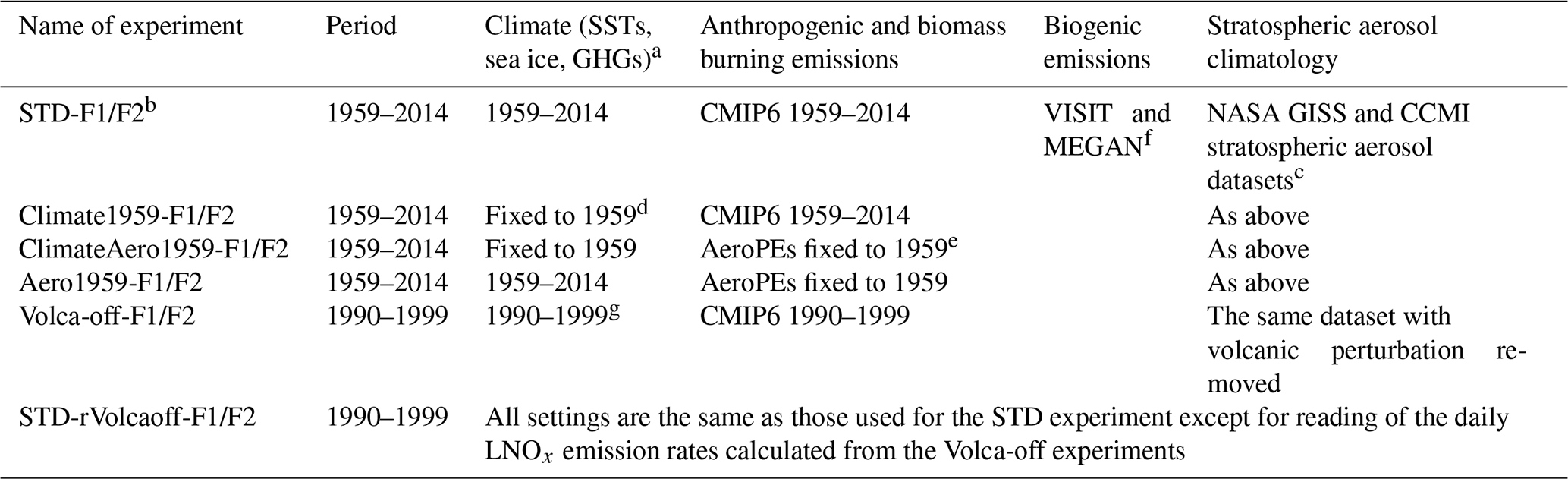
^a For the model simulations, the climate is simulated by the prescribed SSTs and sea ice fields and the prescribed varying concentrations of GHGs (CO₂; N₂O; methane; chlorofluorocarbons, CFCs; and hydrochlorofluorocarbons, HCFCs) used only in the radiation scheme. The SSTs and sea ice fields are obtained from the HadISST dataset (Rayner et al., 2003). The prescribed GHG concentrations are derived from CMIP6 forcing datasets (Meinshausen et al., 2017). ^b We use “F1” to stand for the ECMWF-McCAUL scheme; “F2” represents the CTH scheme. ^c Stratospheric aerosol radiative forcing is simulated using the prescribed stratospheric aerosol extinction, which is obtained from the NASA GISS (Sato et al., 1993) and CCMI (Arfeuille et al., 2013) stratospheric aerosol datasets. ^d The climate is fixed to 1959 for the whole simulation period using the 1959 SSTs and sea ice field and GHG concentrations during the simulation period. ^e Aerosol (BC, OC) and aerosol precursor (NO_x, SO₂) emissions (anthropogenic + biomass burning) are fixed to 1959 throughout the simulation period. ^f Several biogenic emissions are interannually varying, including isoprene, monoterpenes, acetone, and methanol, which were calculated using an offline simulation using the Vegetation Integrative Simulator for Trace Gases (VISIT) terrestrial ecosystem model (Ito and Inatomi, 2012). Some other reactive biogenic VOCs (ethane, propane, ethylene, propene) used are climatological data derived from the Model of Emissions of Gases and Aerosols from Nature (MEGAN) modeling system (Guenther et al., 2012). ^g Here the June 1991–May 1995 SSTs and sea ice data were replaced with HadISST SSTs and sea ice climatological data during 1985–1990.

Download Print Version | Download XLSX

We simulate volcanic aerosol forcing by considering the prescribed stratospheric aerosol extinction in the radiation scheme. We used the NASA Goddard Institute for Space Studies (GISS) (Sato et al., 1993) and the Chemistry–Climate Model Initiative (CCMI) (Arfeuille et al., 2013) stratospheric aerosol datasets as the stratospheric aerosol climate data. The NASA GISS dataset includes monthly zonal-mean stratospheric aerosol optical thickness in four spectral bands. The CCMI dataset for CHASER includes monthly zonal-mean stratospheric aerosol extinction coefficients in 20 spectral bands. To remove the volcanic perturbation while maintaining the stratospheric background aerosol in the Volca-off-F1/F2, we used the following equation to process the stratospheric aerosol climatology (SAC) during June 1991–May 1996.

In this equation, SAC_{no_pinatubo} denotes the stratospheric aerosol climatological data as input data for Volca-off-F1/F2 experiments, and SAC_background represents the stratospheric background aerosol climatological data. (For this study, SAC_background is the corresponding temporally averaged values of the NASA GISS and CCMI stratospheric aerosol datasets during June 1986–May 1991 and June 1996–May 2001, when the time was close to the eruption and the stratosphere was less affected by volcanic eruptions.) SAC_raw stands for the original values of the NASA GISS and CCMI stratospheric aerosol datasets during June 1991–May 1996. Moreover, σ symbolizes the standard deviations of stratospheric background aerosol climate data. (For this study, σ is the corresponding standard deviations of the NASA GISS and CCMI stratospheric aerosol datasets during June 1986–May 1991 and June 1996–May 2001.) As displayed in Eq. (11), when the absolute differences between SAC_raw and SAC_background are larger than 1.96σ, we replace the original values (June 1991–May 1996) of the SAC with the temporally averaged values of the NASA GISS and CCMI datasets during June 1986–May 1991 and June 1996–May 2001. When the absolute differences between SAC_raw and SAC_background are equal to or smaller than 1.96σ, we still use the original values (June 1991–May 1996) of the SAC for the Volca-off experiments. The value of 1.96σ corresponds to the 95 % confidence interval, which can remove the Pinatubo perturbation sufficiently while maintaining the background level of stratospheric aerosol during June 1991–May 1996. Furthermore, the influences of the Pinatubo eruption affected the HadISST SSTs and sea ice fields. To remove the Pinatubo eruption's influences on the SSTs and sea ice fields from the Volca-off experiments too, we replaced the June 1991–May 1995 SSTs and sea ice data with HadISST SSTs and sea ice climatological data during 1985–1990 when conducting the Volca-off experiments. The 1985–1990 period was chosen because it is approximately the period of June 1991–May 1995 and because the SSTs and sea ice fields were less affected by volcanic activity during 1985–1990.

All the experiments calculate the LNO_x emissions rates interactively through LNO_x emission parameterizations except STD-rVolcaoff experiments. The STD-rVolcaoff experiments are the same as the STD experiments except for reading the daily LNO_x emission rates calculated from the Volca-off experiments. The STD-rVolcaoff experiments are conducted for comparison with the STD experiments to elucidate the effects of LNO_x emissions changes caused by the Pinatubo eruption on atmospheric chemistry (typically methane lifetime).

3.1 Validation of the simulated historical lightning distribution and trend

To increase the credibility of the conclusions obtained based only on the numerical simulations, the model calculations must be evaluated using observational data. We used the LIS and OTD observations to evaluate the spatial and temporal distribution and historical lightning trends simulated by CHASER (MIROC). Figure 1a–c show the annual mean spatial distributions of lightning observed by LIS and OTD and by model simulations using the ECMWF-McCAUL and CTH schemes. Both the ECMWF-McCAUL and the CTH schemes generally captured the hotspots of lightning (central Africa, the Maritime Continent, South America) well, with strong spatial correlations between observations and model simulations (R>0.75), even if the lightning distributions were not well captured over the ocean. Figure 1d exhibits a strong spatial correlation between observations and simulation results maintained throughout the simulation period (1959–2014).

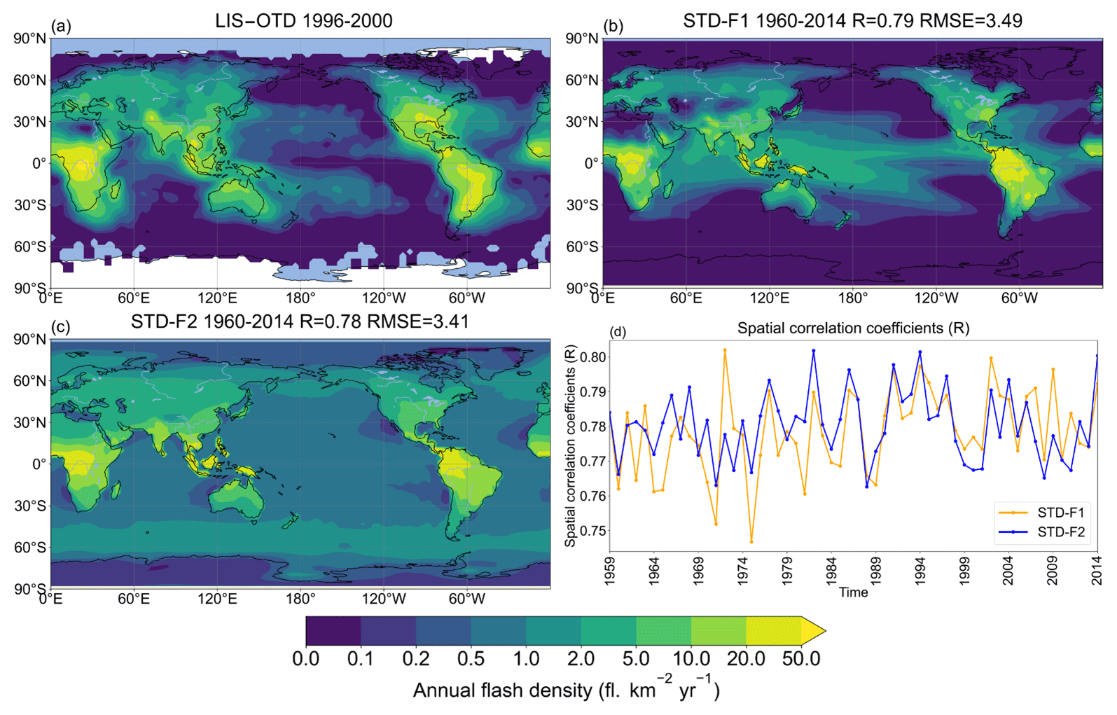
Figure 1Annual mean lightning flash densities from (a) LIS and OTD satellite observations spanning 1996–2000, (b) the STD experiment (1960–2014) with the ECMWF-McCAUL scheme used, and (c) the STD experiment (1960–2014) with the CTH scheme used. R and RMSE as shown in the title of panel (b) are calculated between panels (b) and (a), while R and RMSE as shown in the title of panel (c) are calculated between panels (c) and (a). Panel (d) presents the spatial correlation coefficients between the modeled spatial lightning distribution of each year and LIS and OTD lightning climatologies during 1996–2000.

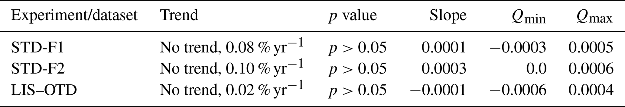
The LIS and OTD observations are also used to evaluate historical lightning trends simulated by CHASER (MIROC). We examined the ±37.5^∘ latitude mean LFR anomaly (1996–2013) calculated from LIS and OTD observations and STD-F1/F2 numerical experiments (Fig. 2 and Table 2). We also note some missing values within the ±37.5^∘ latitude in LIS and OTD observations. To constrain the comparisons between observations and simulations as like-for-like, when we encounter a missing value in the LIS and OTD observations during spatial averaging, we also treat the CHASER-simulated value at the same location as a missing value. As displayed in Fig. 2, we would not necessarily expect that interannual variations in the LFR anomaly can be captured because meteorological nudging was not applied, and the simulated LFRs were only controlled by the prescribed SSTs and sea ice data. Nevertheless, the overall trends in the LFR anomaly simulated using both schemes matched the LIS and OTD observations well, as portrayed in Fig. 2. We further investigated the trends shown in Fig. 2 by the Mann–Kendall rank statistic and Sen's slope estimator, and the statistical summary is displayed in Table 2 (Salmi et al., 2002; Hussain and Mahmud, 2019). Neither the LFR anomaly (within ±37.5^∘ latitude) derived from LIS and OTD observations nor the simulations show a significant trend for 1996–2013 using the Mann–Kendall rank statistic test (significance inferred as 5 %). The global LFR anomaly during 1993–2013 obtained from simulations (STD-F1/F2) also shows no significant trend, which is consistent with the Schumann resonance (SR) intensity observations (1993–2013) at Rhode Island, USA (Williams, 2022). However, the SR observations in Rhode Island (USA) exclude a consideration of the influences of solar cycles, which makes it less appropriate for lightning trend evaluation.

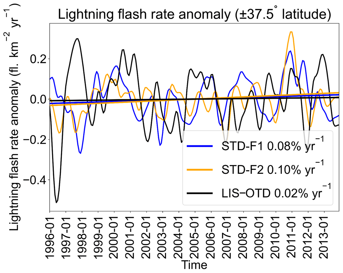
Figure 2LFR anomalies of 1996–2013 within ±37.5^∘ latitude obtained from two numerical experiments (STD-F1/F2) and LIS and OTD satellite observations. The curves represent the monthly time series data of the ±37.5^∘ latitude mean LFR anomalies with the 1-D Gaussian (denoising) filter applied. The lines are the fitting curves of the monthly time series data of the ±37.5^∘ latitude mean LFR anomalies. The trends in the LFR anomalies in percent per year are also presented in the legends.

Download

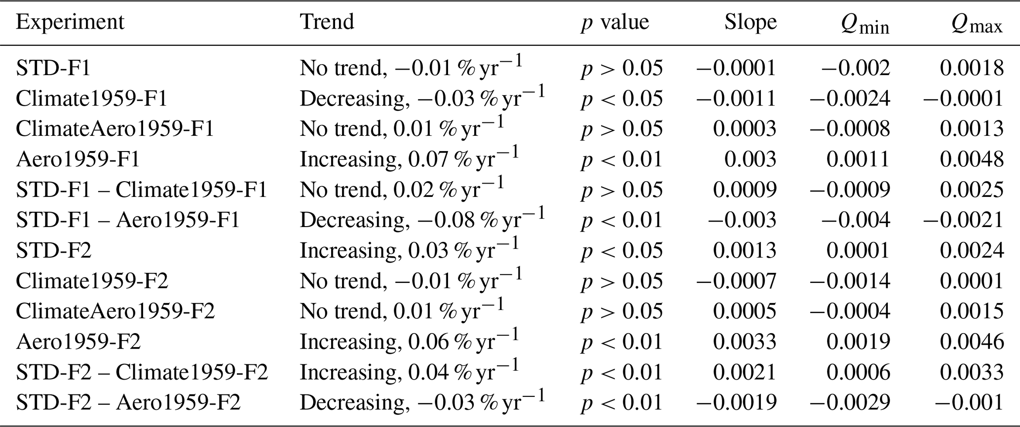
Table 2A statistical summary of the trends shown in Fig. 2 by the Mann–Kendall rank statistic and Sen's slope estimator. The monthly time series data of the ±37.5^∘ latitude mean LFR anomalies were estimated by the Mann–Kendall rank statistic and Sen's slope estimator. “Trend” shows whether these are significant trends with the significance set as 5 %, as well as the percentage trends in percent per year estimated by linear regression. The p value is calculated during the Mann–Kendall trend test. “Slope” shows Sen's slope of trend. Q_min and Q_max respectively denote the lower and upper limits of the 95 % confidence interval of Sen's slope.

Download Print Version | Download XLSX

We further investigated the seasonal variabilities in the simulated LFR and compared them against LIS and OTD observations. The results are depicted in Fig. 3. Both the CTH and the ECMWF-McCAUL schemes captured the peak during JJA, but the overestimation of LFR by F1/F2 during DJF is also noticeable. Figure S1 in the Supplement presents a comparison of the LFR global distribution in different seasons during 1996–2003 from LIS and OTD lightning observations and STD experiment outputs. Generally, CHASER captured the spatial distribution of LFR in all four seasons well when compared against LIS and OTD observations. The spatial correlation coefficients (R) between observations and simulations are the highest (R=0.80 for both lightning schemes) in DJF, indicating CHASER's considerable capability to reproduce the LFR spatial distribution in DJF. As displayed in the first row of Fig. S1, the overestimation of LFR by F1/F2 during DJF is primarily attributable to the overestimation of LFR within the Maritime Continent and South America, but this might also be attributable to the underestimation of LFR by LIS and OTD within these two regions. It is believed that the LIS and OTD lightning detection efficiency is highly sensitive to the characteristics of convective clouds (cloud albedo, cloud optical thickness, etc.) (Boccippio et al., 2002; Cecil et al., 2014). High cloud albedo and cloud optical thickness might engender the underestimation of LFR by LIS and OTD. It is also noteworthy that the seasonal variation and long-term trend of global lightning are strongly influenced by distinct factors. The seasonal variation in global lightning activities is the most strongly affected by the 23^∘ obliquity of the Earth's orbit and the asymmetric distribution of the continent between the Northern Hemisphere and the Southern Hemisphere. However, the long-term global lightning trend we investigated for this study is mainly controlled by climate forcers such as aerosols and GHGs. To minimize the effects of LFR seasonal variation on our study's results, we deseasonalized the results shown in all figures and tables by calculating their anomaly based on raw data. The validation described above and the deseasonalization of our study's results justified that the LFR seasonal variation (and the uncertainties in the simulation of LFR seasonal variation) in our study has a limited effect on these study results.

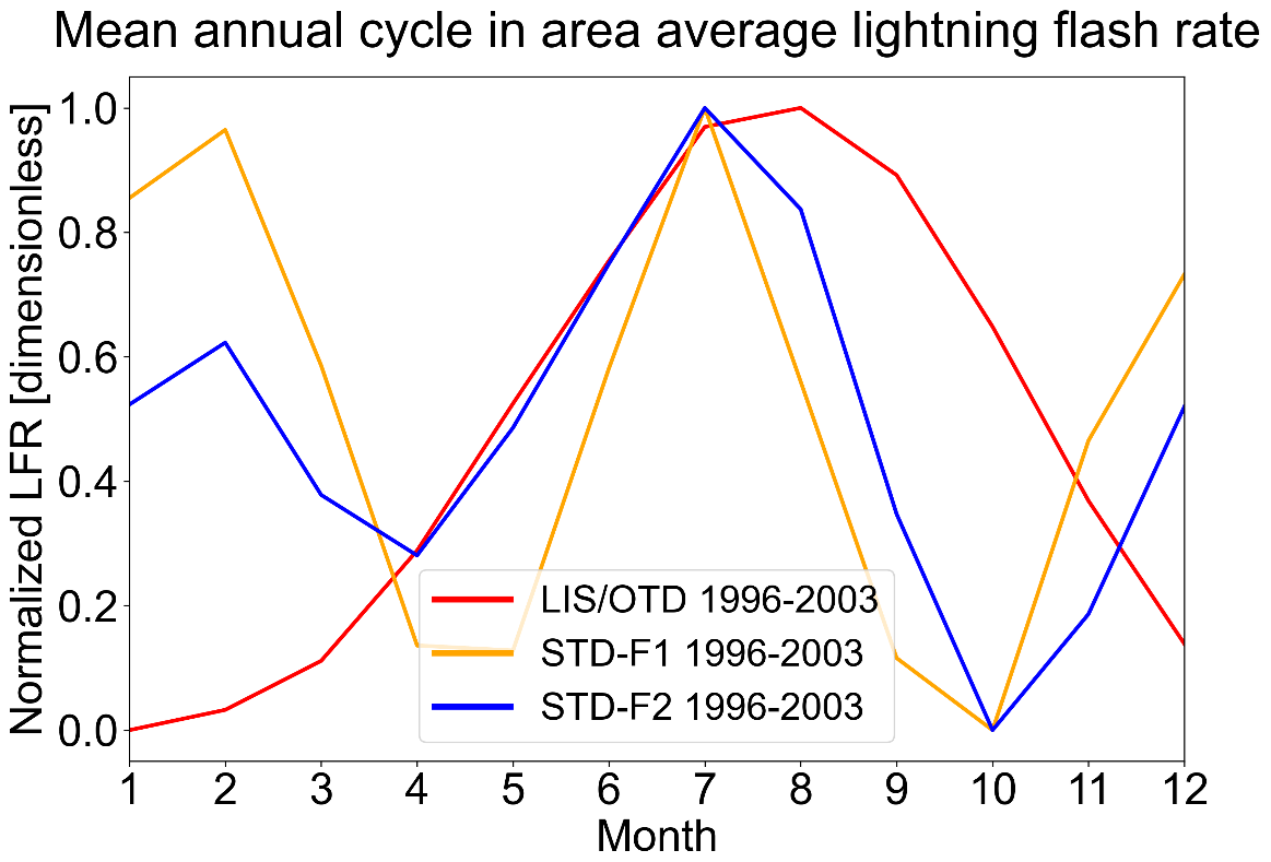
Figure 3The mean annual cycle in the area average LFR during 1996–2003. The area average was taken over the grid cells where valid LIS and OTD lightning observations exist. LFR is normalized by min–max normalization.

Download

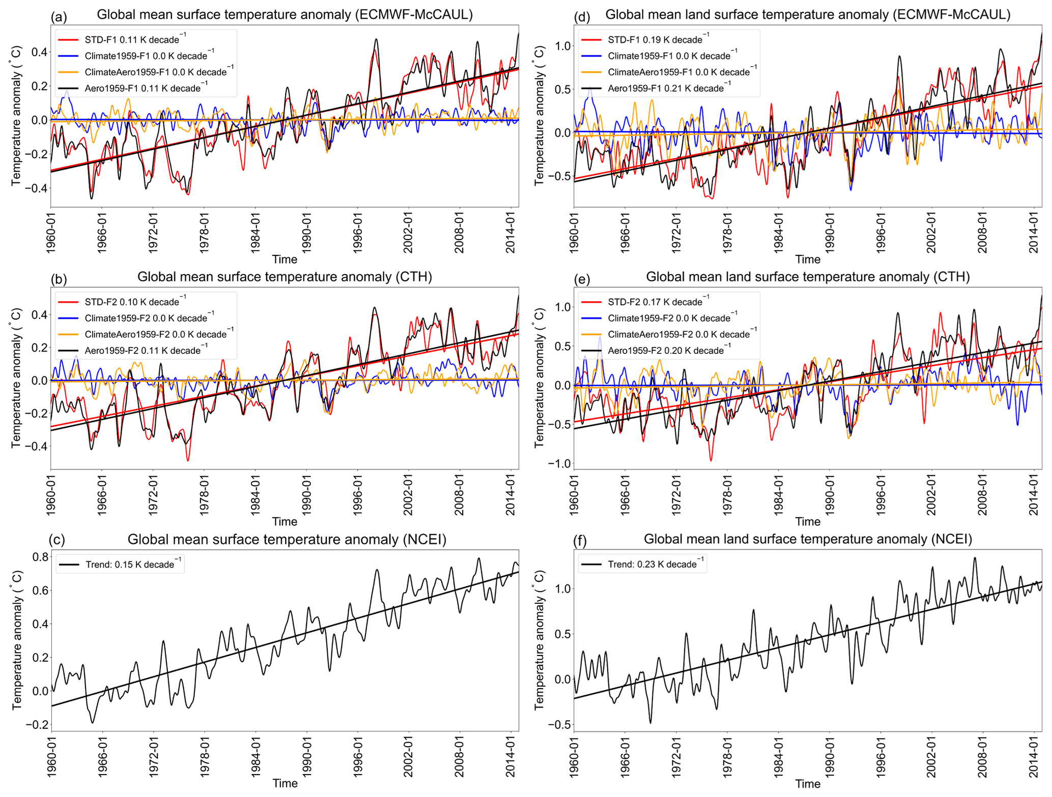
Figure 4Monthly time series data of global mean surface temperature anomalies with the 1-D Gaussian (denoising) filter applied and their fitting curves calculated from the outputs of numerical experiments (a, b) and obtained from NCEI (c). Panels (d–f) are the same as panels (a–c), but the averaged surface temperature anomalies are only calculated within the global land regions. The trends of the fitting curves in kelvin per decade are also presented in the legends.

Download

3.2 Effects of global warming and increases in AeroPEs on historical lightning and LNO_x trends

As introduced in Sect. 1, global warming and changes in AeroPEs are the two main factors which influence long-term (1960–2014) historical lightning trends. (Hereinafter, historical lightning trends represent lightning trends of 1960–2014.) Evidence shows that the Pacific Decadal Oscillation (PDO) can also affect lightning trends over decadal timescales (Macias Fauria and Johnson, 2006; Mallick et al., 2022), and further research is anticipated to verify it. To analyze the effects of global warming on historical lightning trends, we designed and conducted two sets of experiments: one set of experiments including global warming (STD-F1/F2) and another set of experiments excluding global warming (Climate1959-F1/F2). Figure 4a and b respectively depict the global surface temperature anomalies calculated using the ECMWF-McCAUL and CTH schemes. The STD and Aero1959 experiments show an increasing trend (around 0.11 K per decade) of global mean surface temperature anomalies, which closely approximates the trend (around 0.15 K per decade) obtained from NOAA's National Centers for Environmental Information (NCEI) (2022) (Fig. 4c and f). Global temperature change data from 1880 to the present are available from NCEI, which tracks variations in the Earth's temperature based on thousands of stations' observation data around the globe (Climate at a Glance, National Centers for Environmental Information (NCEI), 2022). When the prescribed SSTs and sea ice fields and GHG concentrations were fixed to 1959 throughout the simulation period, the simulated trends of global mean surface temperature anomalies turned out to be flat (Climate1959 and ClimateAero1959). To elucidate the effects of increases in AeroPEs on averaged surface temperature to the greatest extent possible, we also show the averaged surface temperature anomaly only over land regions (Fig. 4d–f). The simulated global mean land surface temperature anomalies are also well matched with the NCEI observational data. The aerosol cooling effect can be more evident when only examining surface temperature trends averaged over land (Fig. 4d and e).

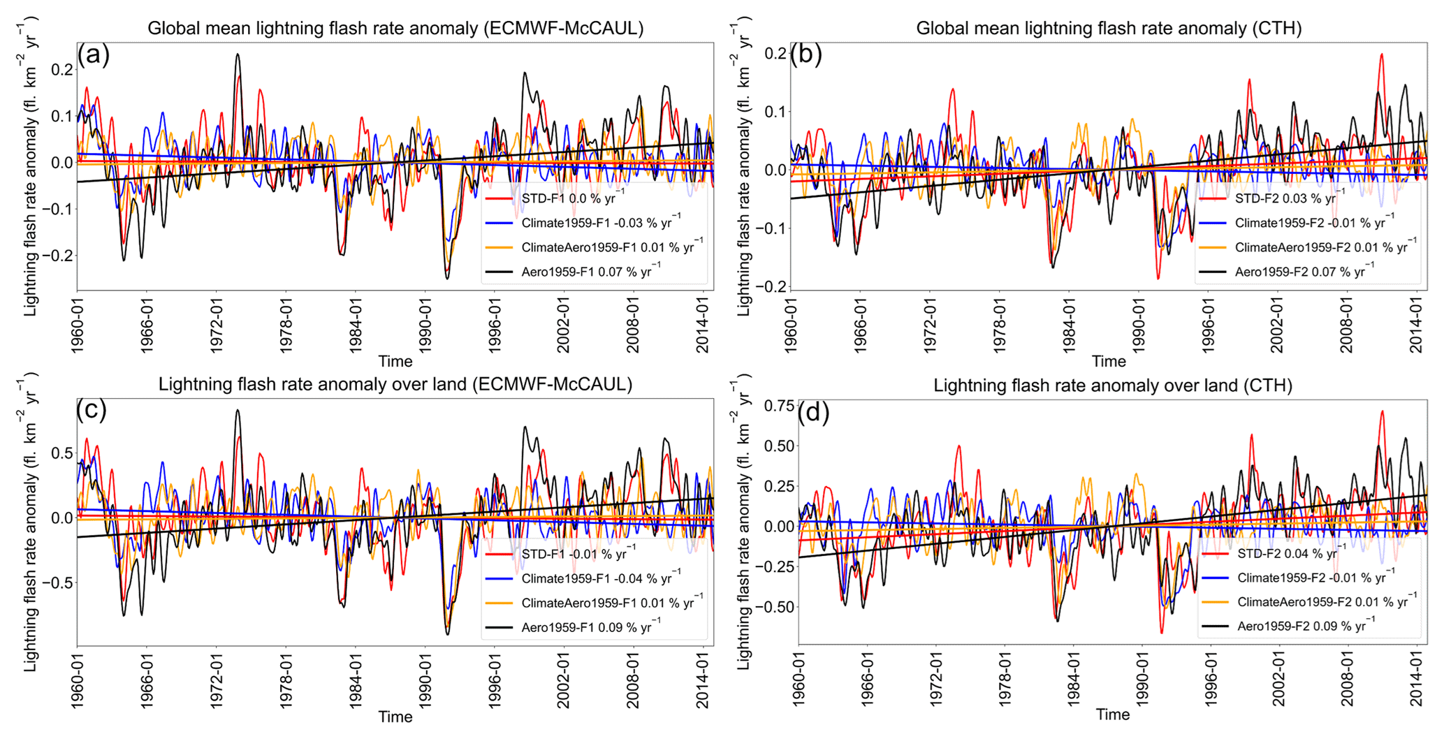
Figure 5Panels (a) and (b) show monthly time series data of global mean LFR anomalies with the 1-D Gaussian (denoising) filter applied and their fitting curves of different experiments simulated respectively using the ECMWF-McCAUL and CTH schemes. Panels (c) and (d) are the same as panels (a) and (b), except for the fact that the averaged LFR anomalies are calculated only within global land regions. Trends of the fitting curves (% yr⁻¹) are also shown in the legends.

Download

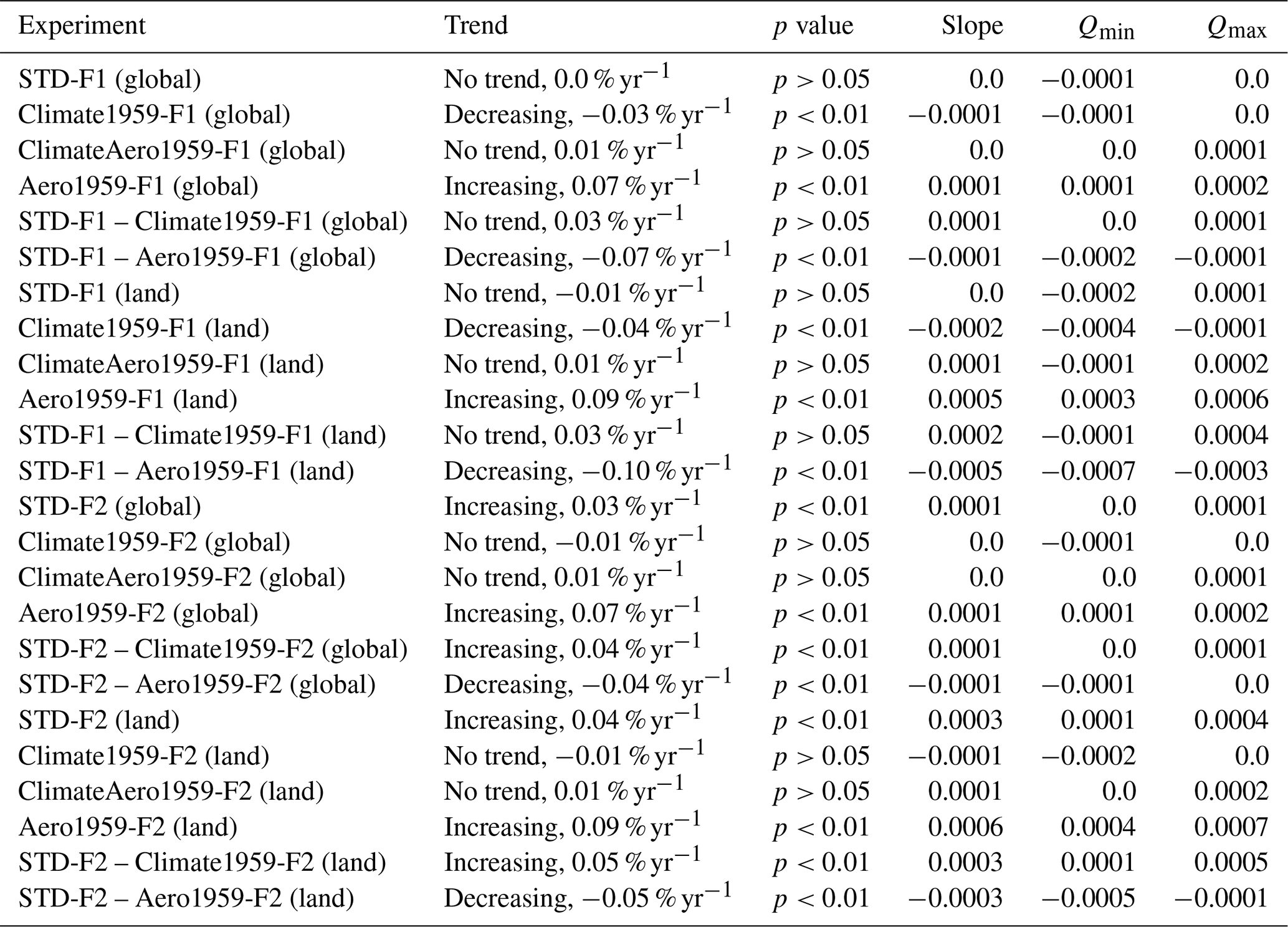
Figure 5a and b respectively portray the global mean LFR anomalies and their fitting curves obtained from the outputs of the ECMWF-McCAUL and CTH schemes. Moreover, Table 3 shows the statistical summary of the trends in Fig. 5 utilizing the Mann–Kendall rank statistic and Sen's slope estimator. The global lightning trend obtained from the STD-F1 experiment turned out to be statistically flat (0.0 % yr⁻¹), whereas the outputs of the STD-F2 experiment exhibited a significant increasing global lightning trend (0.03 % yr⁻¹) determined using the Mann–Kendall rank statistic (significance inferred as 5 %).

Table 3A statistical summary of the trends shown in Fig. 5 by the Mann–Kendall rank statistic and Sen's slope estimator. The monthly time series data of global or land mean LFR anomalies were estimated by the Mann–Kendall rank statistic and Sen's slope estimator. “Trend” shows whether these are significant trends with the significance set as 5 %, as well as the percentage trends in percent per year estimated by linear regression. The p value is calculated during the Mann–Kendall trend test. “Slope” shows Sen's slope of trend. Q_min and Q_max respectively denote the lower and upper limits of the 95 % confidence interval of Sen's slope.

Download Print Version | Download XLSX

A comparison of the lightning trends calculated from the STD and Climate1959 experiments showed that both lightning schemes demonstrated that historical global warming (1960–2014) enhances the global lightning trends toward positive trends (around 0.03 % yr⁻¹ or 3 % K⁻¹). Global warming effects on historical lightning trends were evaluated as significant using the Mann–Kendall rank statistic, with significance inferred as 5 %, when using the CTH scheme but not in the case of the ECMWF-McCAUL scheme (see rows STD-F1 – Climate1959-F1 (global) and STD-F2 – Climate1959-F2 (global) in Table 3). As shown in Table 3, the differences in global lightning trends simulated by the STD-F1/F2 and Aero1959-F1/F2 experiments indicate that the increases in AeroPEs during 1960–2014 significantly suppress the global lightning trends (−0.07 % to −0.04 % yr⁻¹). It is noteworthy that this suppression of lightning trends is only attributable to aerosol radiative effects. Further research must be conducted to elucidate the long-term effects of aerosols on lightning through aerosol microphysical effects. We also investigated lightning trends only over land regions (Fig. 5c and d and Table 3) to ascertain the effects of changes in AeroPEs to the greatest extent possible. When observing the lightning trends over land only, the degree of suppression of lightning trends attributable to increases in AeroPEs expands to −0.10 % to −0.05 % yr⁻¹, which is attributable to most AeroPEs and their growth coming from land regions. It is noteworthy that we used the same SSTs and sea ice data in the Aero1959 as those used for STD experiments. The SSTs and sea ice data also reflected the effects of increases in AeroPEs. Therefore, we might underestimate the effects of increases in AeroPEs on lightning trends by comparing the results of STD and Aero1959 experiments.

For the ECMWF-McCAUL scheme, model outputs affirm that global warming can enhance the global mean CAPE anomaly slightly and suppress the global mean Q_Ra anomaly (Fig. 6a and b). Earlier studies have also indicated that the total solid (cloud ice, snow, and graupel) mass mixing ratio within charge separation regions is lower under global warming. Moreover, possible explanations are given in those studies (Finney et al., 2018; Romps, 2019). Because global warming enhances global convection activities and because lightning formation is highly related to convection activity, global warming enhances the historical global lightning trend simulated using the ECMWF-McCAUL scheme, mainly as a result of the simulated CAPE trend, which is enhanced by global warming.

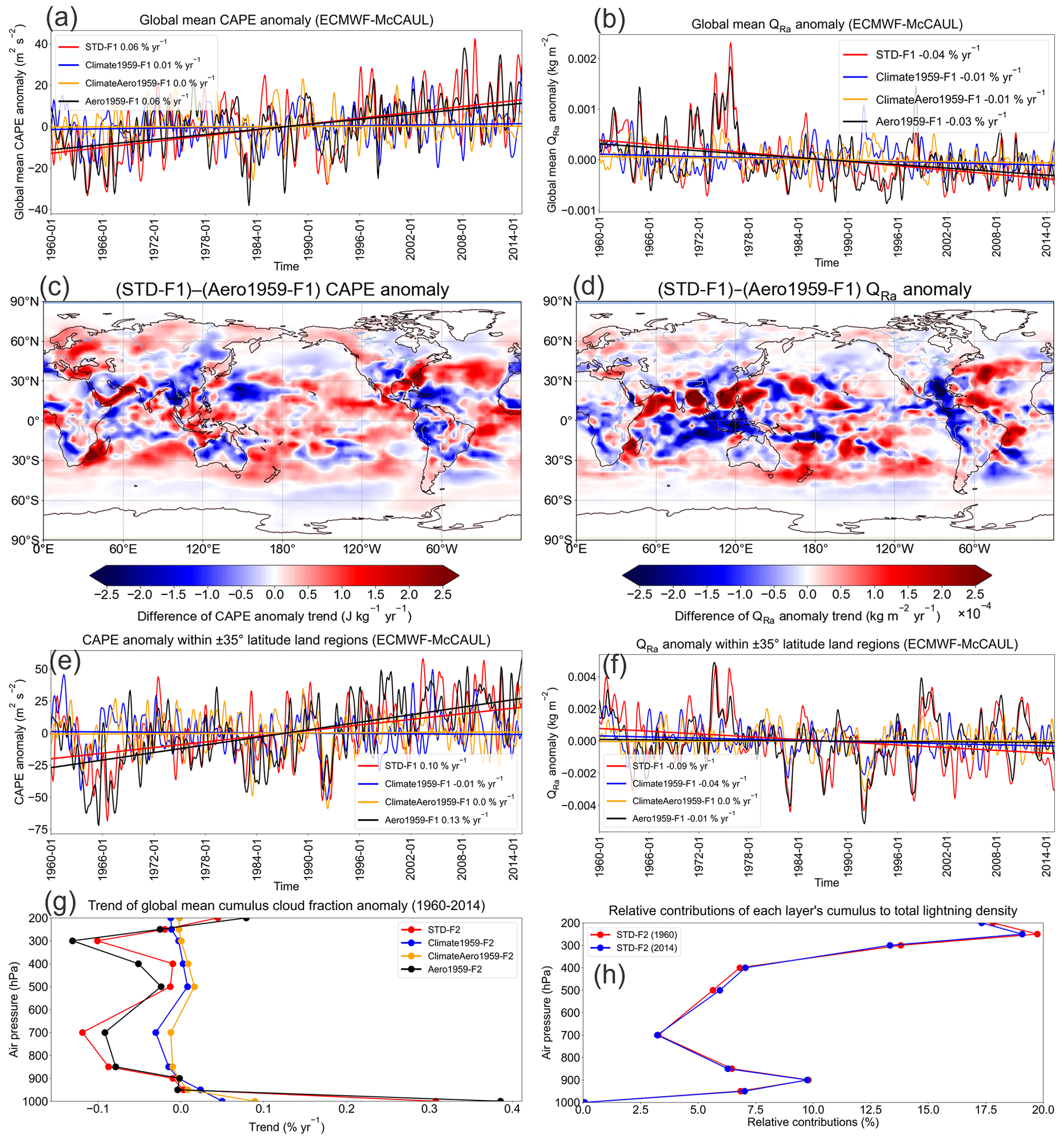
Figure 6Panels (a) and (b) respectively show monthly time series data of the global mean CAPE and Q_Ra anomalies with the 1-D Gaussian (denoising) filter applied and their fitting curves simulated using the ECMWF-McCAUL scheme. Panels (c) and (d) respectively show differences in the CAPE anomaly trend ($\mathrm{J}{\mathrm{kg}}^{-\mathrm{1}}{\mathrm{yr}}^{-\mathrm{1}}$) and Q_Ra anomaly trend ($\mathrm{kg}{\mathrm{m}}^{-\mathrm{2}}{\mathrm{yr}}^{-\mathrm{1}}$) of the STD-F1 and Aero1959-F1 experiments in the global map. Panels (e) and (f) respectively show monthly time series data of the ±35^∘ latitude land region mean CAPE and Q_Ra anomalies with the 1-D Gaussian (denoising) filter applied and their fitting curves simulated using the ECMWF-McCAUL scheme. Panel (g) portrays the vertical profiles of the trend of the global mean cumulus cloud fraction anomaly simulated by the CTH scheme. Panel (h) depicts the relative contributions of each layer's cumulus to total lightning density in 1960 and 2014, as calculated from the outputs of the STD-F2 experiment.

The past increases in AeroPEs exert negligible effects on the trends of global mean CAPE and Q_Ra anomalies, as displayed in Fig. 6a and b. However, as also demonstrated in our study (see Fig. 1), most lightning flashes occur over tropical and subtropical land regions. It is displayed in Fig. 6c and d that the past increases in AeroPEs mostly suppress the CAPE and Q_Ra absolute trends within regions with high lightning densities. We further investigated the trends of the ±35^∘ latitude land region mean CAPE and Q_Ra anomalies, and the results are portrayed in Fig. 6e and f. Figure 6e and f show that past increases in AeroPEs significantly suppress the Q_Ra trend (−0.08 % yr⁻¹) and slightly suppress the CAPE trend (−0.03 % yr⁻¹) within ±35^∘ latitude land regions. Weaker convection activities (smaller CAPE) and fewer hydrometeors (cloud ice, graupel, snow) in the charge separation regions (0 to −25 ^∘C isotherm) engender less lightning. In the case of the ECMWF-McCAUL scheme, CAPE and Q_Ra trends were suppressed within ±35^∘ latitude terrestrial regions. This constitutes the main reason for the suppression of the historical global lightning trends induced by increases in AeroPEs through aerosol radiative effects. It is noteworthy that, because the aerosol microphysical effects are only considered in the grid-scale large-scale condensation scheme, our study might underestimate the aerosol microphysical effects which can enhance the trends of Q_Ra and LFR toward a positive direction.

To explain the results simulated by the CTH scheme, we investigated the vertical profiles of the trend of the global mean cumulus cloud fraction anomaly (Fig. 6g). Investigating cumulus cloud fraction is reasonable because each model layer's cumulus cloud fractions are used to weight the calculated lightning densities from that layer in the CTH scheme, as introduced in Eqs. (3) and (4). Figure 6h shows the relative contributions of each model layer's cumulus to the calculated global total lightning densities in 1960 and 2014 obtained using the CTH scheme. As is shown in Fig. 6h, the vertical profiles of the relative contribution in 1960 and 2014 are almost identical. Cumulus convection is positively correlated with lightning formation, which is the scientific basis of parameterizing lightning densities using the cumulus cloud top height: the CTH scheme. Historical global warming enhances the lightning trend simulated by the CTH scheme mainly because the simulated historical global warming increases the cumulus reaching 200 hPa, which contributes greatly to the simulated global total lightning density (Fig. 6g and h). The increases in the deep convective cloud are regarded as related to the increases in tropopause height attributable to global warming, as shown in Fig. S2 in the Supplement. The past increases in AeroPEs suppress the lightning trend simulated by the CTH scheme because increases in AeroPEs decrease the cumulus reaching 200 hPa as well as the cumulus within the lower to middle troposphere by aerosol radiative effects (Fig. 6g). In addition, in the Supplement, we present a figure (Fig. S3) resembling Fig. 6 but which includes only a consideration of land regions. The mechanisms of global warming and increases in AeroPEs affecting lightning trends over land regions are similar to those described above on a global scale. We do not discuss details of them here.

We also investigated lightning trends simulated in different experiments with the global map (Fig. 7). Both the ECMWF-McCAUL and the CTH schemes show that lightning increased significantly in most parts of the Arctic region and decreased in some parts of the Southern Ocean during 1960–2014 (Fig. 7a and e). The significant lightning trends presented in Fig. 7a became nearly nonexistent when the climate simulations were fixed to 1959 (Fig. 7b and f), indicating the considerable effects of global warming on the trend of global lightning activities. Furthermore, the effects of past global warming and increases in AeroPEs on the lightning trends on the global map are displayed in Fig. 8. Figure 8a and c show that past global warming enhances lightning activities within the Arctic region and Japan, which is consistent with findings of an earlier study from which thunder day data in Japan were reported (Fujibe, 2017). Figure 8a and c also show that historical global warming suppresses lightning activities around New Zealand and some parts of the Southern Ocean. Both lightning schemes demonstrated that the historical increases in AeroPEs suppress lightning activities in some parts of the Southern Ocean and South America. The ECMWF-McCAUL scheme also suggests that historical increases in AeroPEs suppress lightning activities by aerosol radiative effects in some parts of India and China, where AeroPEs increased dramatically during 1960–2014 because of rapid economic development and energy consumption. Many observation-based studies indicate that aerosols can invigorate lightning activities in some regions of China and India, typically under relatively clean conditions (e.g., AOD<1.0), which is attributable to the aerosol microphysical effects (Wang et al., 2011; Zhao et al., 2017, 2020; Lal et al., 2018; Liu et al., 2020; Shi et al., 2020). Therefore, a total positive effect of aerosol on historical lightning trends in China and India cannot be ruled out. We further provided the same figures as Figs. 7 and 8 but using different units ($\mathrm{fl}.{\mathrm{km}}^{-\mathrm{2}}{\mathrm{yr}}^{-\mathrm{2}}$) in Figs. S4 and S5 in the Supplement. Figures S4 and S5 show that the absolute lightning trends ($\mathrm{fl}.{\mathrm{km}}^{-\mathrm{2}}{\mathrm{yr}}^{-\mathrm{2}}$) and the effects of global warming and increases in AeroPEs on the absolute lightning trends are slight in high-latitude regions but prominent in tropical areas.

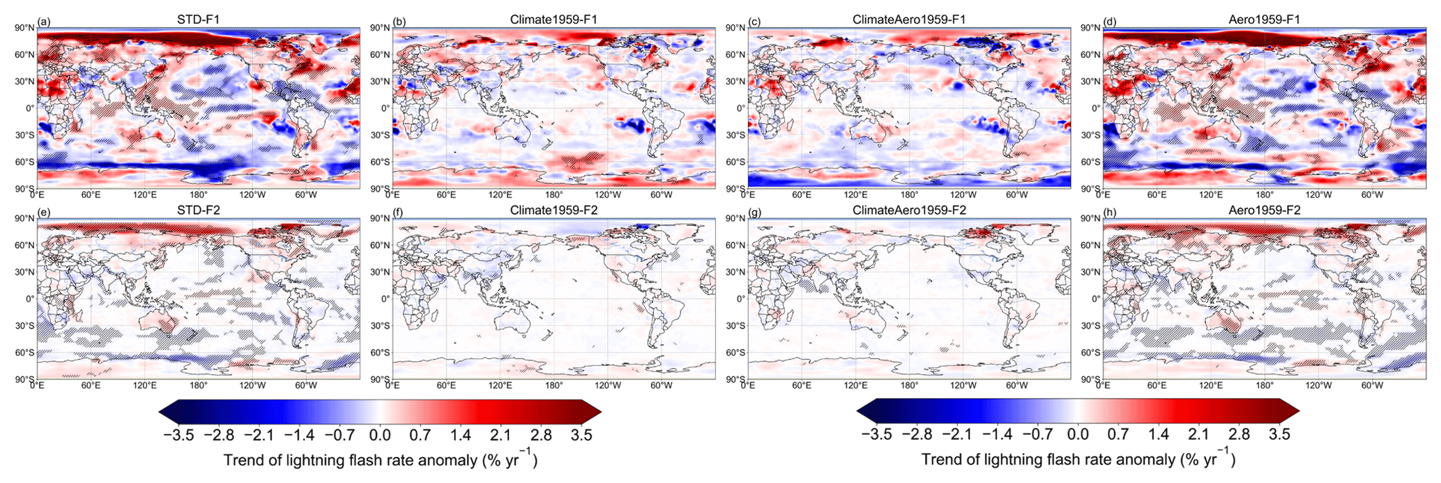
Figure 7Trends of the LFR anomaly (% yr⁻¹) during 1960–2014 on the 2-D map. The trend at every point was calculated from the function of the approximating curve for the 1960–2014 time series data (LFR anomaly) at each grid cell. The area in which the trend was found to be significant by the Mann–Kendall rank statistic test (significance inferred as 5 %) is marked with the hatched lines.

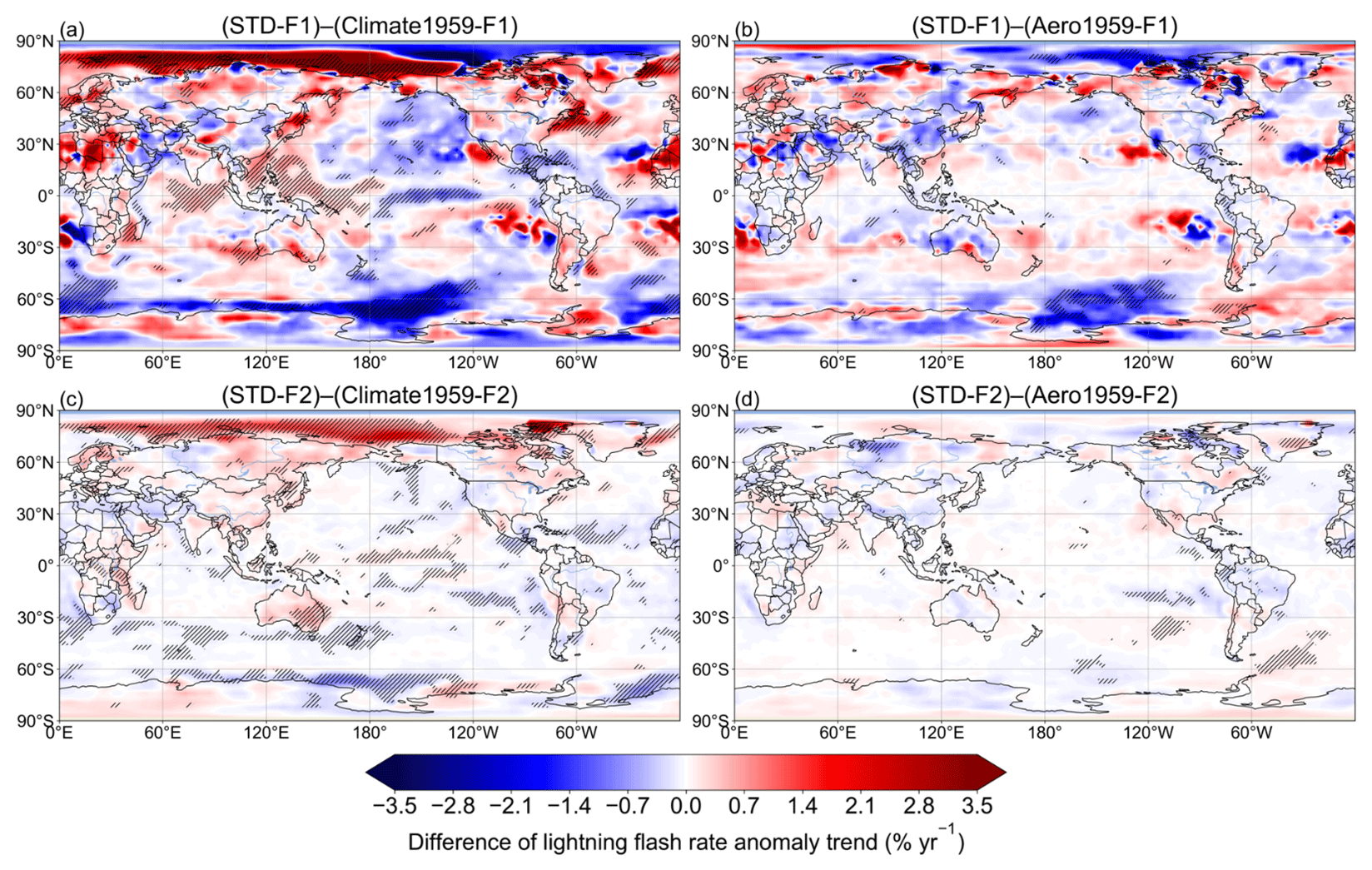
Figure 8Differences in trends of the LFR anomaly during 1960–2014 on the global map. The area in which the trend of the differences in the LFR anomaly time series data was found to be significant by the Mann–Kendall rank statistic test (significance inferred as 5 %) is marked with the hatched lines.

Trends in historical annual global LNO_x emissions for different scenarios are generally consistent with trends in historical global mean LFRs, as shown in Figs. 5a and b and 9. This finding is not surprising because, as the lightning NO_x emission parameterizations introduced in Sect. 2.2 show, the simulated LFRs are linearly related to the simulated LNO_x emissions in our study. A comparison of the LNO_x trends calculated from the STD and Climate1959 experiments showed that both lightning schemes demonstrated that historical global warming (1960–2014) enhances the global LNO_x trends toward positive trends (0.02 %–0.04 % yr⁻¹). Global warming effects on historical LNO_x trends were evaluated as significant using the Mann–Kendall rank statistic, with significance inferred as 5 %, when using the CTH scheme but not in the case of the ECMWF-McCAUL scheme (see rows STD-F1 – Climate1959-F1 and STD-F2 – Climate1959-F2 in Table 4). As shown in Table 4, the differences in global LNO_x trends simulated by the STD and Aero1959 experiments indicate that the increases in AeroPEs during 1960–2014 significantly suppress the global LNO_x trends (−0.08 % to −0.03 % yr⁻¹). The results presented in Fig. 9 and Table 4 imply that historical global warming and increases in AeroPEs can affect atmospheric chemistry and engender feedback by influencing LNO_x emissions.

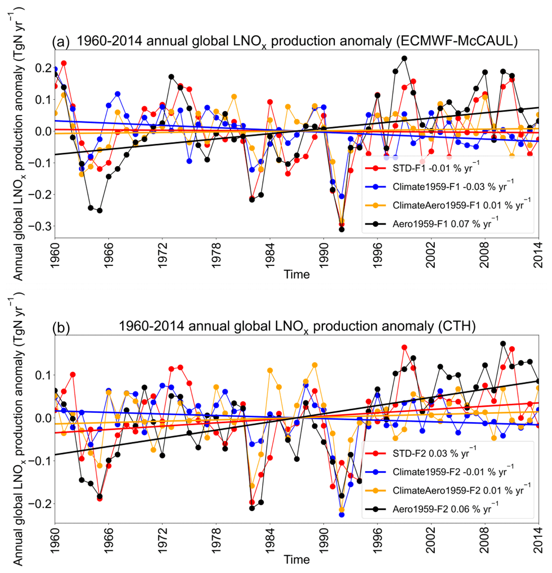
Figure 9Time series data of the 1960–2014 annual global LNO_x production anomalies (Tg N yr⁻¹) and their fitting curves simulated using the ECMWF-McCAUL (a) and CTH schemes (b). Trends of the fitting curves in percent per year are presented in the legends.

Download

Table 4A statistical summary of the trends shown in Fig. 9 by the Mann–Kendall rank statistic and Sen's slope estimator. The time series data of the annual global LNO_x production anomalies were estimated by the Mann–Kendall rank statistic and Sen's slope estimator. “Trend” shows whether these are significant trends with the significance set as 5 %, as well as the percentage trends in percent per year estimated by linear regression. The p value is calculated during the Mann–Kendall trend test. “Slope” shows Sen's slope of trend. Q_min and Q_max respectively denote the lower and upper limits of the 95 % confidence interval of Sen's slope.

Download Print Version | Download XLSX

3.3 Pinatubo volcanic eruption effects on historical lightning and LNO_x trends

We estimate the Pinatubo eruption effects on historical lightning and LNO_x trends and variation by comparing the simulation results of the STD and Volca-off experiments. The simulated global mean LFRs by the STD and Volca-off experiments are the same until April 1991. They then begin to show differences from May 1991 (the time series of the global mean LFRs is not shown). This result is reasonable because the Pinatubo volcanic perturbations are removed from the SAC during June 1991–May 1996 in the Volca-off experiments in Eq. (11) and because the SAC of May 1991 used in CHASER is interpolated between the SAC of April 1991 and June 1991.

Figure 10c and d portray the time series of the LFR anomalies and Relative_diff (values over the red lines) during 1991–1992. Relative_diff is the relative difference in the global mean LFR anomalies between the STD and Volca-off experiments calculated using the following equation.

In the equation, LFRA_STD represents the global mean LFR anomalies simulated by the STD-F1/F2 experiments. LFRA_Volca-off denotes the global mean LFR anomalies simulated by the Volca-off-F1/F2 experiments. LFR_Volca-off symbolizes the global mean LFRs simulated by the Volca-off-F1/F2 experiments.

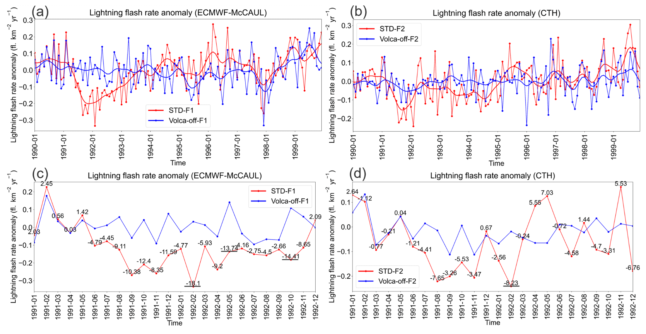
Figure 10Time series of the LFR anomalies during 1990–1999 and 1991–1992. Panels (a) and (b) show the time series of the LFR anomalies and their smoothed curves by the 1-D Gaussian (denoising) filter for 1990–1999. Panels (c) and (d) present the time series of the LFR anomalies during 1991–1992. The values shown over the red lines in panels (c) and (d) are Relative_diff calculated using Eq. (12).

Download

The monthly time series data of Relative_diff for 1990–1999 for both lightning schemes are calculated. The probability density distributions (PDDs) of Relative_diff spanning 1990–1999 and June 1991–May 1992 are displayed in Fig. 11. The 1990–1999 Relative_diff values presented in Fig. 11 (colored blue) are all normally distributed as determined by the Kolmogorov–Smirnov test. The 95 % confidence interval of the 1990–1999 Relative_diff is calculated and shown in the titles of Fig. 11. As displayed in Fig. 10c and d, the underlined values (Relative_diff) exceeded the 95 % confidence interval, indicating significant differences in the calculated global mean LFR anomalies by the STD and Volca-off experiments. In other words, global lightning activities were suppressed significantly by the Pinatubo eruption during the first year after the eruption. The PDDs of the June 1991–May 1992 Relative_diff (colored green in Fig. 11) shifted to the left compared to the 1990–1999 PDDs, indicating that global lightning activities were suppressed in the first year after the eruption.

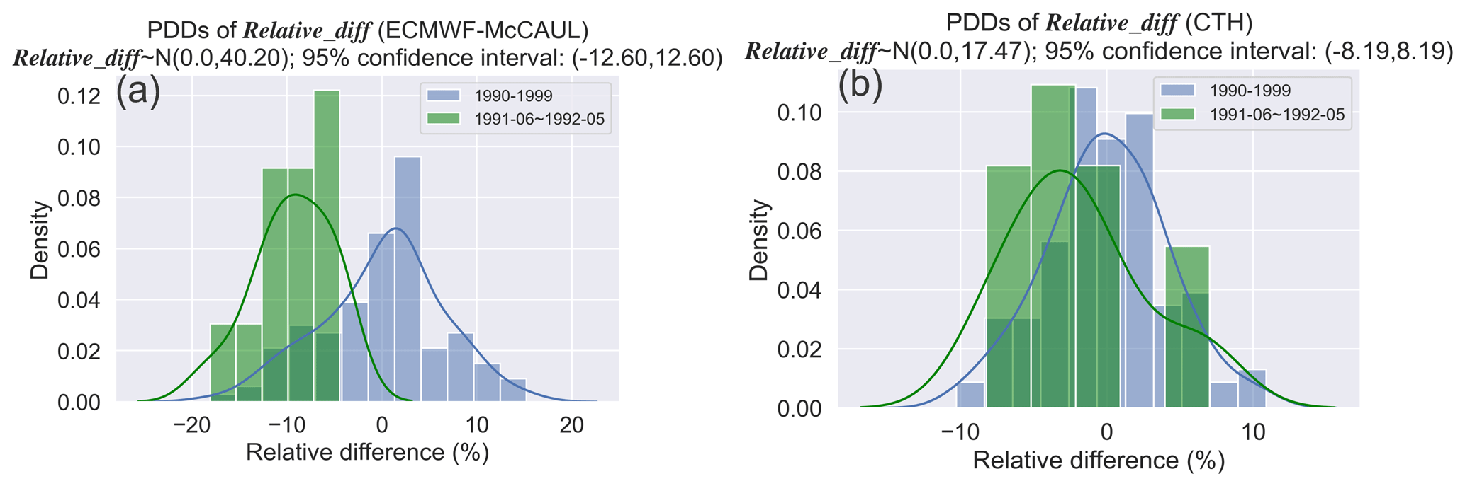
Figure 11Probability density distributions (PDDs) of Relative_diff obtained from monthly time series data of Relative_diff during 1990–1999 and June 1991–May 1992 (a year after the Pinatubo eruption). The 1990–1999 Relative_diff for both lighting schemes is normally distributed, and N(μ,σ²) is displayed in the titles of this figure. The 95 % confidence interval of the 1990–1999 Relative_diff is also shown in the titles of this figure.

Download

Figure 12a and b show August 1991–April 1992 averaged LFR anomaly differences between the STD and Volca-off experiments on the global map. We found from Fig. 12a and b that lightning activities are suppressed significantly within the three hotspots of lightning activities (central Africa, the Maritime Continent, and South America) during August 1991–April 1992, when the global mean LFRs are found to be suppressed. To elucidate the potential reasons for the suppressed global lightning activities during the first year after the Pinatubo eruption, we first investigated the August 1991–April 1992 averaged differences in the CAPE and Q_Ra anomalies between STD-F1 and Volca-off-F1 (Fig. 12c and d) because lightning densities are computed with CAPE and Q_Ra by the ECMWF-McCAUL scheme. The results showed that the Pinatubo eruption can engender apparent reductions in CAPE and Q_Ra within tropical and subtropical terrestrial regions (typically three hotspots of lightning activities) where lightning occurrence is frequent. These reductions constitute the main reason for the suppressed global lightning activities during the first year after the Pinatubo eruption simulated by the ECMWF-McCAUL scheme. We also examined the August 1991–April 1992 averaged differences of the 200–400 hPa averaged cumulus cloud fraction anomaly between STD-F2 and Volca-off-F2 on the global map (Fig. 12e). The cumulus cloud fractions of each model layer are used to weight the calculated lightning densities from that layer by the CTH scheme, as explained in Sect. 2.2. As depicted in Figs. 12e and S6 in the Supplement, the Pinatubo eruption led to marked reductions in the middle to upper tropospheric cumulus cloud fractions during August 1991–April 1992 over three hotspots of lightning activities (central Africa, the Maritime Continent, and South America). As displayed in Fig. 6h, the cumulus that reached the middle to upper troposphere is closely related to lightning formation. Consequently, the simulated global lightning activities by the CTH scheme were also suppressed considerably during the first year after the Pinatubo eruption.

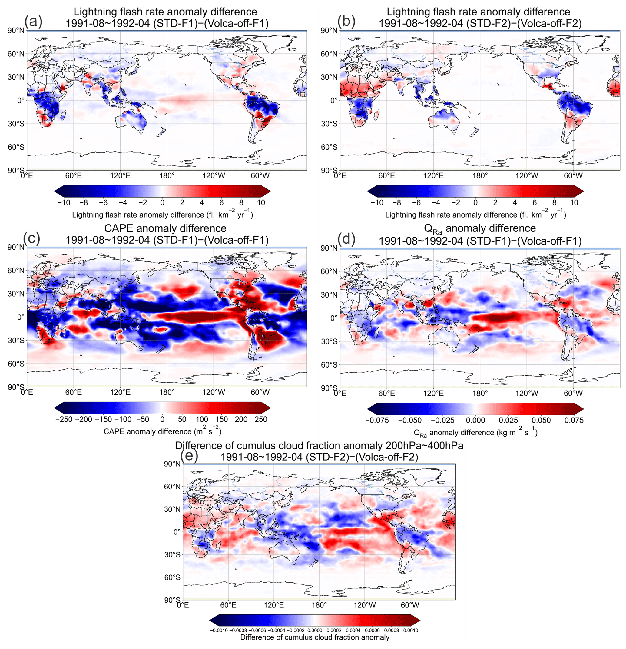
Figure 12The August 1991–April 1992 averaged LFR anomaly differences (a, b), CAPE anomaly differences (c), Q_Ra anomaly differences (d), and differences of the 200–400 hPa averaged cumulus cloud fraction anomaly between the STD-F2 and Volca-off-F2 experiments (e) on the global map.

Aside from the global lightning activity suppression described earlier, the production of LNO_x might also decrease after the Pinatubo eruption. To explore this conjecture, we compared the LNO_x emissions in the STD and Volca-off experiments (Fig. 13). In the case of the ECMWF-McCAUL scheme, the reduction in LNO_x emissions caused by the Pinatubo eruption started in 1991 (5.84 %) and continued until 1993, with the highest percentage reduction occurring in 1992 (8.47 %) (Fig. 13a). However, the CTH scheme showed a slightly different scenario of LNO_x emissions reduction after the Pinatubo eruption. The LNO_x emissions are almost evenly reduced during 1991–1994 in the case of the CTH scheme (Fig. 13b). In conclusion, our study indicates that the Pinatubo eruption can engender reductions in global LNO_x emissions, which last 2–3 years. However, there exists some uncertainty in evaluating the magnitude of the reductions: from 1.99 % to 8.47 % for the annual percentage reduction found in our study.

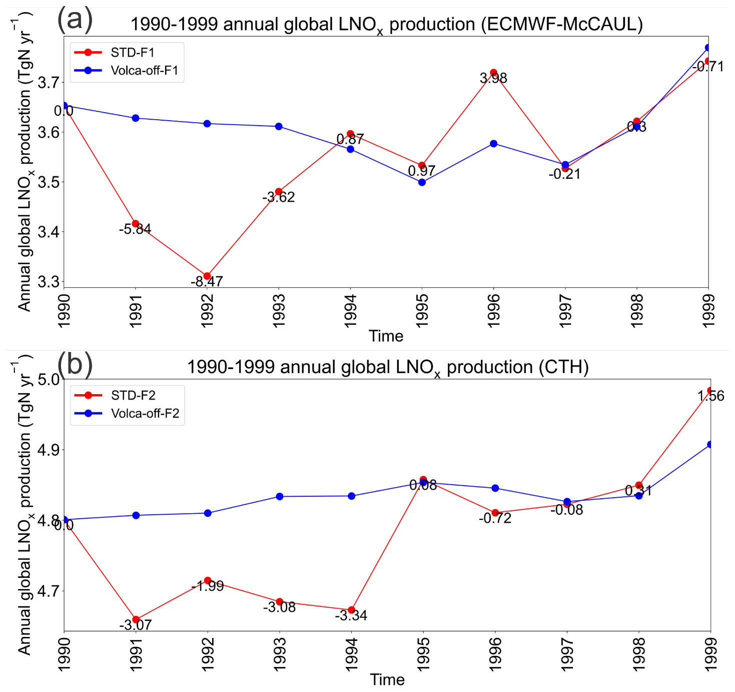
Figure 13The 1990–1999 annual global LNO_x emissions calculated from the STD and Volca-off experiments' outputs simulated using the ECMWF-McCAUL (a) and CTH schemes (b). Values over the red lines represent the relative differences (%) between the red and blue lines, calculated with respect to the blue lines.

Download

The simulated reduced global LNO_x emissions caused by the Pinatubo eruption might influence atmospheric chemistry significantly. Most importantly, the reduced global LNO_x emissions might reduce OH radical production and extend the global mean tropospheric lifetime of methane against tropospheric OH radicals, abbreviated hereinafter as the methane lifetime. We investigated this point further by comparing the methane lifetime anomaly simulated by the STD and STD-rVolcaoff experiments. As introduced in Sect. 2.5, the settings of the STD-rVolcaoff experiments are the same as those use for the STD experiments, except that they use the daily LNO_x emission rates calculated from the Volca-off experiments. We calculated the monthly CH₄ lifetime anomalies during 1990–1999 and $\mathrm{\Delta }{\mathit{\tau }}_{{\mathrm{CH}}_{\mathrm{4}}}$ (the difference in the CH₄ lifetime anomaly between the STD and STD-rVolcaoff experiments), which are shown in Fig. 14c and d. Figure 14a and b display the PDDs of $\mathrm{\Delta }{\mathit{\tau }}_{{\mathrm{CH}}_{\mathrm{4}}}$ monthly time series during 1990–1999. The $\mathrm{\Delta }{\mathit{\tau }}_{{\mathrm{CH}}_{\mathrm{4}}}$ values shown in Fig. 14a and b are all normally distributed, as determined using the Kolmogorov–Smirnov test. The 95 % confidence interval of $\mathrm{\Delta }{\mathit{\tau }}_{{\mathrm{CH}}_{\mathrm{4}}}$ is calculated and shown in the titles of Fig. 14a and b. The annual global LNO_x production averaged during 1990–1999 is 3.56 Tg N yr⁻¹ for STD-F1 and 4.79 Tg N yr⁻¹ for STD-F2. At this level of annual global LNO_x production, we found that within the first 2 years after the Pinatubo eruption, $\mathrm{\Delta }{\mathit{\tau }}_{{\mathrm{CH}}_{\mathrm{4}}}$ exceeded the 95 % confidence interval simulated by both lighting schemes (February 1992 and April 1992 in the case of the ECMWF-McCAUL scheme; December 1991 in the case of the CTH scheme). However, the widely cited range of annual global LNO_x production is 2–8 Tg N yr⁻¹ (Schumann and Huntrieser, 2007). Presuming that $\mathrm{\Delta }{\mathit{\tau }}_{{\mathrm{CH}}_{\mathrm{4}}}$ responds linearly to the LNO_x emission level and that the annual global LNO_x production is 8 Tg N yr⁻¹, then the extension of the CH₄ lifetime because of the reduced LNO_x emissions can reach around 0.54 years for the ECMWF-McCAUL scheme. As a comparison, ultraviolet shielding effects caused by stratospheric aerosols after the Pinatubo eruption led to the maximum increase in the methane lifetime by about 0.6 years (Fig. 14c and d).

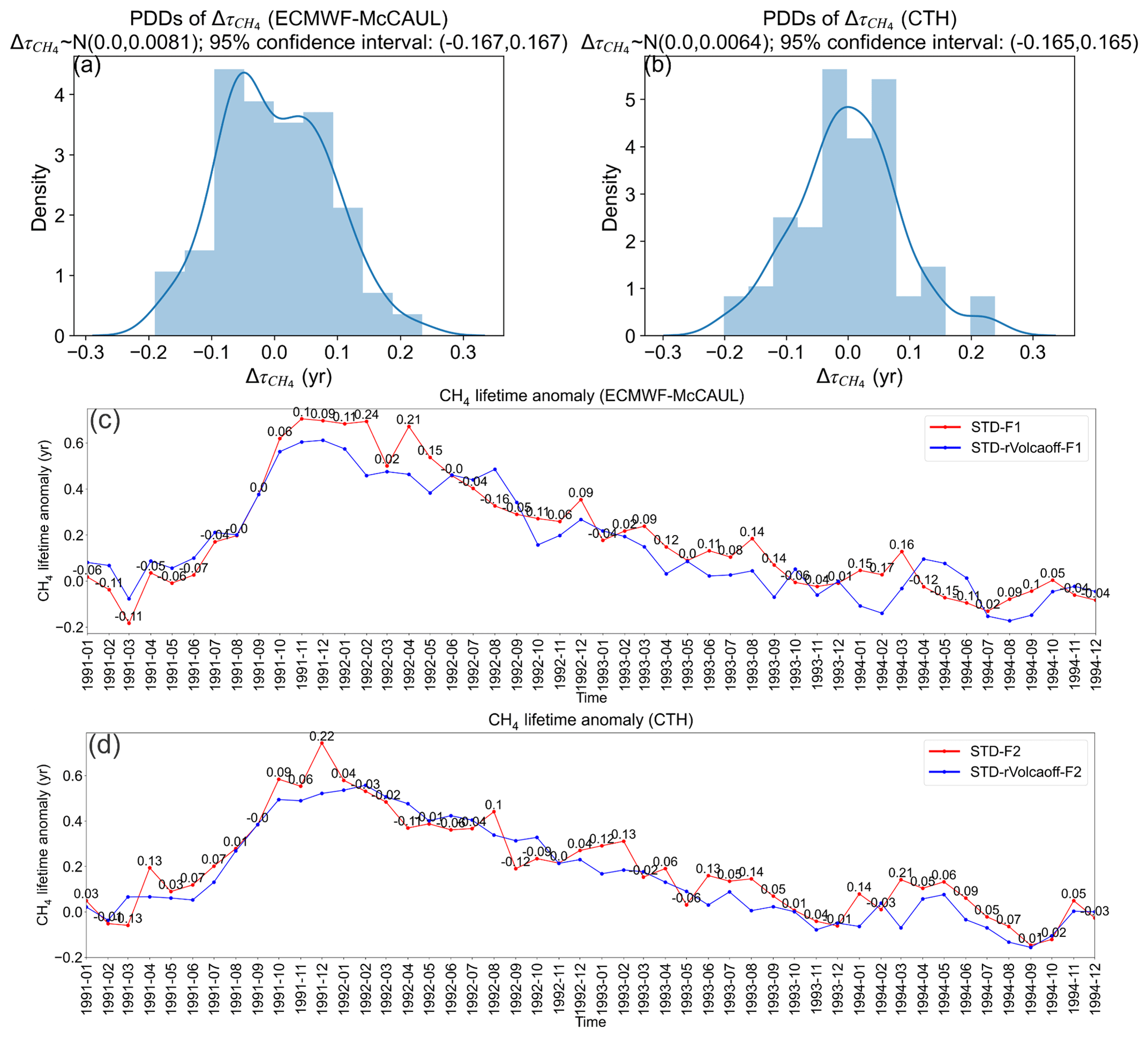
Figure 14Panels (a) and (b) show the probability density distributions (PDDs) of $\mathrm{\Delta }{\mathit{\tau }}_{{\mathrm{CH}}_{\mathrm{4}}}$ obtained from the monthly time series data of $\mathrm{\Delta }{\mathit{\tau }}_{{\mathrm{CH}}_{\mathrm{4}}}$ during 1990–1999. $\mathrm{\Delta }{\mathit{\tau }}_{{\mathrm{CH}}_{\mathrm{4}}}$ represents the difference in the CH₄ lifetime anomaly between the STD and STD-rVolcaoff experiments. The 95 % confidence interval of $\mathrm{\Delta }{\mathit{\tau }}_{{\mathrm{CH}}_{\mathrm{4}}}$ is also presented in the titles of panels (a) and (b). Panels (c) and (d) show monthly time series of the CH₄ lifetime anomalies simulated by the STD-F1/F2 and STD-rVolcaoff-F1/F2 experiments. The values over the red lines represent $\mathrm{\Delta }{\mathit{\tau }}_{{\mathrm{CH}}_{\mathrm{4}}}$.

Download

3.4 Model intercomparisons of LFR trends with CMIP6 model outputs

The historical lightning trends demonstrated in our study are undoubtedly worth comparing with the results of other chemistry–climate models or Earth system models. As introduced in Sect. 2.4, for comparison of the simulated LFR trends and variations in our study with those of other CMIP6 models' outputs, we used all available LFR data from the CMIP6 CMIP historical experiments from CESM2-WACCM (3 ensembles) (Danabasoglu, 2019), GISS-E2-1-G (9 ensembles) (Kelley et al., 2020), and UKESM1-0-LL (18 ensembles) (Tang et al., 2019). Table S1 presents a complete list of the ensemble members we used. It is noteworthy that the LFR data obtained from the three CMIP6 models described earlier are calculated using the CTH scheme. The results of model intercomparisons of LFR trends and variations are displayed in Fig. 15.

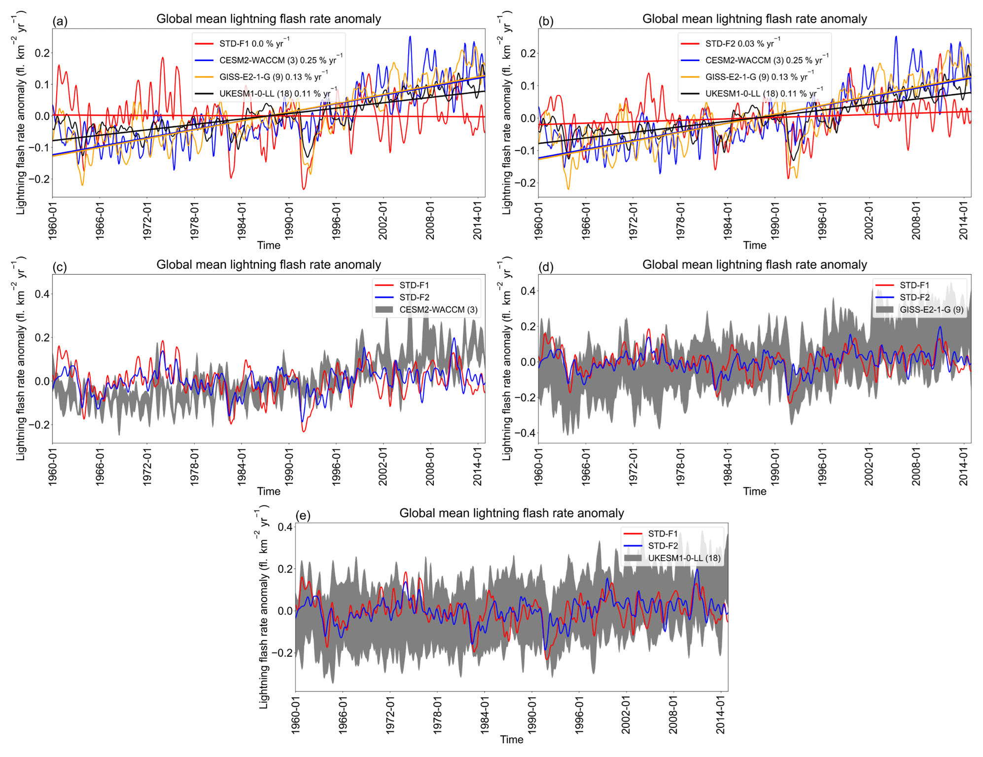
Figure 15Comparisons of simulated global mean LFR anomalies found in our study (CHASER) and found using other CMIP6 models. All the figures are created based on the monthly time series data of global mean LFR anomalies with a 1-D Gaussian (Denoising) filter applied. For CMIP6 models, the ensemble mean is shown as the solid line, and the full ensemble range is shown as grey shading (c–e). Fitting curves and the trends of fitting curves (% yr⁻¹) are also given in (a and b).

Download

As displayed in Fig. 15a and b and Table 6, both the ECMWF-McCAUL and the CTH schemes (STD-F1/F2) simulated almost flat global lightning trends (even the trend is estimated to be significant in the case of the CTH scheme (0.03 % yr⁻¹)), but the ensemble means obtained from another three CMIP6 models exhibit much larger significant increasing global lightning trends (trends from 0.11 % to 0.25 % yr⁻¹). Many reasons underlie the differences in the global lightning trends simulated by CHASER in our study and by the three CMIP6 models, including the use of different methods to determine SSTs and sea ice fields. Instead of using a coupled atmosphere–ocean general circulation model to calculate SSTs and sea ice fields dynamically in the three CMIP6 models, CHASER uses the prescribed HadISST data (Rayner et al., 2003), which are based on plenty of observational data. Changes in the global mean sea surface temperature anomaly during 1960–2014 (ΔSST) obtained from the STD-F1/F2 and CMIP6 model outputs are presented in Table 5. We also used the observation-based Extended Reconstructed SST (ERSST) dataset (Huang et al., 2017) constructed by NOAA to evaluate the ΔSST obtained from different models. The ΔSST calculated from ERSST during 1960–2014 is 0.549 ^∘C, which most closely approximates the ΔSST obtained from STD-F1/F2. Considered from the perspective of SSTs and sea ice fields alone, the results (global lightning trends) of our study are expected to be closer to the actual situation.

Table 5Changes in the global mean surface temperature anomaly (ΔTS), global mean sea surface temperature anomaly (ΔSST), and global mean lightning flash rate anomaly (ΔLFR), as well as the rate of change in the LFR anomaly corresponding to each degree Celsius increase in the global mean surface temperature anomaly (ΔLFR$/\mathrm{\Delta }$TS) obtained from the STD-F1/F2 and CMIP6 model outputs. The change in ΔSST obtained from the ERSST dataset is also shown in this table. Changes were obtained by calculating the difference between the rightmost and leftmost points of the approximating curve for the 1960–2014 time series data.

Download Print Version | Download XLSX

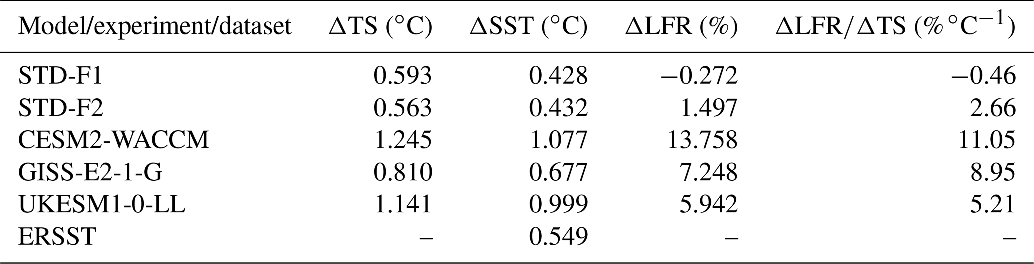
Actually, the three CMIP6 models simulated stronger global warming during 1960–2014 than CHASER in our study, as displayed in Fig. S7 in the Supplement and Table 5. The CTH scheme is reported to respond positively to simulated global warming (Price and Rind, 1994; Zeng et al., 2008; Hui and Hong, 2013; Banerjee et al., 2014; Krause et al., 2014; Clark et al., 2017). The simulated stronger global warming by the three CMIP6 models is regarded as being responsible for differences in the simulated global lightning trends between our study and the three CMIP6 models (Fig. 15a and b and Table 6). We further investigated the sensitivities of the global mean LFR anomaly change to the global mean surface temperature anomaly increase ($\mathrm{\%}{}^{\circ }{\mathrm{C}}^{-\mathrm{1}}$) obtained from CHASER and the three CMIP6 models. The sensitivities in percentage per degrees Celsius are presented in Table 5. Overall, even when using the same CTH scheme, the sensitivities (ΔLFR$/\mathrm{\Delta }$TS) simulated by the three CMIP6 models are higher than those simulated by CHASER in our study. This different sensitivity might be partially attributable to the nonlinear relation between lightning response and climate change (Pinto, 2013; Krause et al., 2014). Compared to the CTH scheme, the ECMWF-McCAUL scheme simulated a statistically non-significant negative sensitivity (ΔLFR$/\mathrm{\Delta }$TS), which is attributable to the stronger suppression of positive global lightning trends caused by increases in AeroPEs simulated using the ECMWF-McCAUL scheme.

Table 6A statistical summary of the trends shown in Fig. 15a and b by Mann–Kendall rank statistic and Sen's slope estimator. The time series data of global mean LFR anomalies were estimated by Mann–Kendall rank statistic and Sen's slope estimator. “Trend” shows whether these are significant trends with the significance set as 5 %, as well as the percentage trends in % yr⁻¹ estimated by linear regression. The p value is calculated during Mann–Kendall trend test. “Slope” shows Sen's slope of trend. Q_min and Q_max respectively denote the lower and upper limits of the 95 % confidence interval of Sen's slope.

Download Print Version | Download XLSX

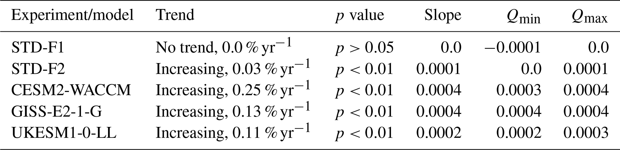
Figure 15d and e affirm that the global lightning variation simulated by our study is basically within the full ensemble range of GISS-E2-1-G and UKESM1-0-LL. After the Pinatubo eruption, as described in Sect. 3.3 of this paper, the GISS-E2-1-G and UKESM1-0-LL models also manifest significant suppression of global lightning activities, but the CESM2-WACCM model shows no such phenomenon. The commonalities and differences in the global lightning trends and variations found in the model intercomparisons imply that great uncertainties existed in past (1960–2014) global lightning trend simulations. Such uncertainties deserve to be investigated further.