the Creative Commons Attribution 4.0 License.
the Creative Commons Attribution 4.0 License.
 | 11 Oct 2023
Total ozone variability and trends over the South Pole during the wintertime
Vitali Fioletov
Xiaoyi Zhao
Ihab Abboud
Michael Brohart
Akira Ogyu
Reno Sit
Sum Chi Lee
Irina Petropavlovskikh
Koji Miyagawa
Bryan J. Johnson
Patrick Cullis
John Booth
Glen McConville
C. Thomas McElroy
The Antarctic polar vortex creates unique chemical and dynamical conditions when the stratospheric air over Antarctica is isolated from the rest of the stratosphere. As a result, stratospheric ozone within the vortex remains largely unchanged for a 5-month period from April until late August when the sunrise and extremely cold temperatures create favorable conditions for rapid ozone loss. Such prolonged stable conditions within the vortex make it possible to estimate the total ozone levels there from sparse wintertime ozone observations at the South Pole. The available records of focused Moon (FM) observations by Dobson and Brewer spectrophotometers at the Amundsen–Scott South Pole Station (for the periods 1964–2022 and 2008–2022, respectively) as well as integrated ozonesonde profiles (1986–2022) and MERRA-2 reanalysis data (1980–2022) were used to estimate the total ozone variability and long-term changes over the South Pole. Comparisons with MERRA-2 reanalysis data for the period 1980–2022 demonstrated that the uncertainties of Dobson and Brewer daily mean FM values are about 2.5 %–4 %. Wintertime (April–August) MERRA-2 data have a bias with Dobson data of −8.5 % in 1980–2004 and 1.5 % in 2005–2022. The mean difference between wintertime Dobson and Brewer data in 2008–2022 was about 1.6 %; however, this difference can be largely explained by various systematic errors in Brewer data. The wintertime ozone values over the South Pole during the last 20 years were about 12 % below the pre-1980s level; i.e., the decline there was nearly twice as large as that over southern midlatitudes. It is probably the largest long-term ozone decline aside from the springtime Antarctic ozone depletion. While wintertime ozone decline over the pole has hardly any impact on the environment, it can be used as an indicator to diagnose the state of the ozone layer, particularly because it requires data from only one station. Dobson and ozonesonde data after 2001 show a small positive, but not statistically significant, trend in ozone values of about 1.5 % per decade that is in line with the trend expected from the concentration of the ozone-depleting substances in the stratosphere.
- Article
(7741 KB) - Full-text XML
- BibTeX
- EndNote


The wintertime stratosphere circulation is dominated by a large cyclonic vortex centered near the pole. A very strong polar vortex in the Antarctic stratosphere creates unique chemical and dynamic conditions and isolates stratospheric air over Antarctica from the rest of the stratosphere (Nash et al., 1996). It forms in austral autumn, reaches maximum strength in midwinter, and breaks down in November–December (Waugh and Polvani, 2010). The variability of the Antarctic vortex is small (Waugh and Randel, 1999) except during the spring vortex breakdown in late spring–summer, although there are some rare exceptions of earlier vortex disruptions. For example, the vortex broke up in September 2002 (Allen et al., 2003; Hoppel et al., 2003; Ricaud et al., 2005), and it demonstrated a large disturbance as early as late August in 1988 (Johnson et al., 2023) and 2019 (Wargan et al., 2020; Safieddine et al., 2020; Milinevsky et al., 2020). Nevertheless, for a period of 5 months, from April to late August, there is a strong undisturbed vortex over the South Pole where ozone is isolated from the rest of the stratosphere and therefore remains relatively unchanged during the wintertime.
The Southern Hemisphere springtime polar vortex has been a subject of intense research since the discovery and subsequent studies of the Antarctic ozone hole (Farman et al., 1985; Solomon et al., 1986; Stolarski et al., 1986). In austral spring, a unique combination of cold temperature, sunlight, polar stratospheric clouds, and a substantial concentration of ozone-depleting substances over Antarctica lead to a very rapid destruction of ozone in the lower stratosphere (e.g., Solomon et al., 1986; WMO, 2018, 2022, and references therein). The wintertime ozone in the vortex is less studied. First, no photochemical ozone destruction processes occur during the polar night, and therefore no rapid changes in ozone are expected. Second, the most reliable satellite ozone instruments, for example the Solar Backscatter Ultraviolet Radiometer (e.g., McPeters et al., 2013), derive column ozone from backscattered solar radiation and therefore cannot measure wintertime column ozone during the polar night.
Long-term ozone trends over the South Pole in the wintertime should be a good indication of the ozone layer state. There was a declining annual total ozone trend in the Southern Hemisphere in the 1980s and early 1990s with a strong latitudinal gradient toward the pole from near-zero trends over the Equator to a total decline of about 8 % at 60∘ S between 1979 and 1996 (e.g., Vyushin et al., 2007; Weber et al., 2018) with little dependence of the season except for the springtime ozone hole (e.g., Fioletov et al., 2002). Similarly, the ozone recovery trends after 1996 are also increasing from the Equator toward high latitudes (Weber et al., 2022). Therefore, from such a latitudinal gradient in the trends, it can be expected that the wintertime ozone changes are the largest over the South Pole.
Unlike the North Pole, the South Pole is practically always under the Antarctic polar vortex during winter (Karpetchko et al., 2005; Waugh and Polvani, 2010). Therefore, measurements from only one location, the Amundsen–Scott South Pole Station, can provide information on the state of the wintertime ozone layer within the polar vortex. Wintertime total ozone measurements at the South Pole Station are available from Dobson and Brewer spectrophotometers that use the Moon as the light source (Komhyr et al., 1988; McElroy et al., 2010) as well as from ozonesondes, from which total ozone can be obtained by integrating the ozone profile (e.g., Johnson et al., 2023).
Information about wintertime ozone over the South Pole Station is also available from the recent Modern-Era Retrospective Analysis for Research and Applications, Version 2 (MERRA-2) reanalysis (Gelaro et al., 2017). The advantage of MERRA-2 is that it provides a continuous record for the period 1980–2022 with an hourly temporal resolution. Every Dobson and Brewer measurement and ozonesonde flight can be matched with a nearly coincident MERRA-2 value to identify potential problems with data and study sampling effects.
The paper is organized as follows. Section 2 describes the datasets used: ground-based ozone measurements by the Dobson and Brewer instruments, total ozone from integrated ozonesondes, and the MERRA-2 reanalysis total ozone data. Section 3 discusses available datasets, differences between them, and possible corrections for the data. Wintertime total ozone variability and long-term changes are discussed in Sect. 4. A discussion and conclusions are given in Sect. 5.
2.1 Dobson spectrophotometer, 1964–2022
The Dobson spectrophotometer was developed in the 1920s and continuous regular measurements started, first in Europe in the 1920s (Dobson and Harrison, 1926; Dobson, 1968) and later in other parts of the globe (Brönnimann et al., 2003). In Antarctica, Dobson measurements started during the International Geophysical Year in 1957–1958. About 130 instruments were produced and about 50 Dobson stations remain operational today (Fioletov et al., 2008) including 6 in Antarctica. Antarctic Dobson measurements led to the discovery of large springtime ozone depletion over Antarctica, or the ozone hole (Farman et al., 1985; Bhartia and McPeters, 2018): anomalous total ozone behavior was uncovered from Dobson measurements at the Japanese station Syowa (Chubachi, 1984) and British station Hally Bay (Farman et al., 1985). Dobson measurements at the South Pole Station started in late 1963. It turns out that some of the early Dobson data recorded there were incorrect, presumably caused by operator error, and were later retracted and reprocessed (Komhyr et al., 1986; Bhartia and McPeters, 2018). Large springtime Antarctic ozone depletion was then further confirmed (Komhyr et al., 1988, 1989b).
The Dobson instrument description, as well as information on its uncertainties, calibration, and operation procedures, can be found in several publications (e.g., Komhyr, 1980; Basher, 1982; Komhyr et al., 1989a; Komhyr and Evans, 2008). The instrument uses three wavelength pairs designated as A (A1:305.5/A2:325.0 nm), C (C1:311.5/C2:332.4 nm), and D (D1:317.5/D2:339.9 nm), and double-pair combinations (typically AD and CD) are used to retrieve total ozone to minimize the optical effect of atmospheric aerosols. The resultant ozone values from the AD and CD combinations do not always agree and instructions to account for this difference are described in the standard operating procedures (Komhyr and Evans, 2008).
A well-known source of potential biases in Dobson measurements is related to the effects of temperature and vertical ozone profile on the derived Dobson total ozone. It is because the standard Dobson retrievals are based on the assumption of a standard stratospheric temperature of −46.3 ∘C and a standard ozone profile (Komhyr et al., 1993), and the ozone absorption (and therefore the total ozone amount) is calculated based on these assumptions. In the case of the South Pole Station, such assumptions could lead to systematic errors of up to 4 % (Bernhard et al., 2005). Redondas et al. (2014) suggested a correction for Dobson systematic errors that was applied by Evans et al. (2017), and such a corrected version of South Pole data was used in this study (see also https://gml.noaa.gov/aftp/data/ozwv/Dobson/Publications/ for details, last access: 10 April 2023). The correction is based on the effective temperature climatology calculated from the ozone and temperature climatological profiles by McPeters and Labow (2012). Note that this version is available from NOAA and is different from the version available from the World Ozone and Ultraviolet Radiation Data Centre (WOUDC, http://woudc.org, last access: 10 February 2023).
Dobson measurements at the South Pole Station are taken using the direct irradiance from the Sun (DS), the Moon (FM), or scattered light from the zenith sky (ZS). Only DS and FM measurements are used in this study. Due to the Sun position in the sky, DS data are available from October to early March, while only FM measurements are available for the rest of the year. There are typically 10–30 measurements per day and one of them is reported as a representative daily value. The Dobson data processing system selects one of the daily observations as representative based on the type of the observation (direct Sun or direct Moon over the zenith sky), wavelength pair (i.e., AD over CD), height of the Sun or Moon (i.e., the observation with the smallest zenith angle is preferred), and interference of clouds (clear sky over cloudy conditions). Most of the South Pole measurements were taken by Dobson instruments 80 and 82 with a short period of measurements by Dobson 42 as shown in Fig. 1. All these Dobsons are calibrated against the world primary Dobson standard instrument 83 (Komhyr et al., 1989a).
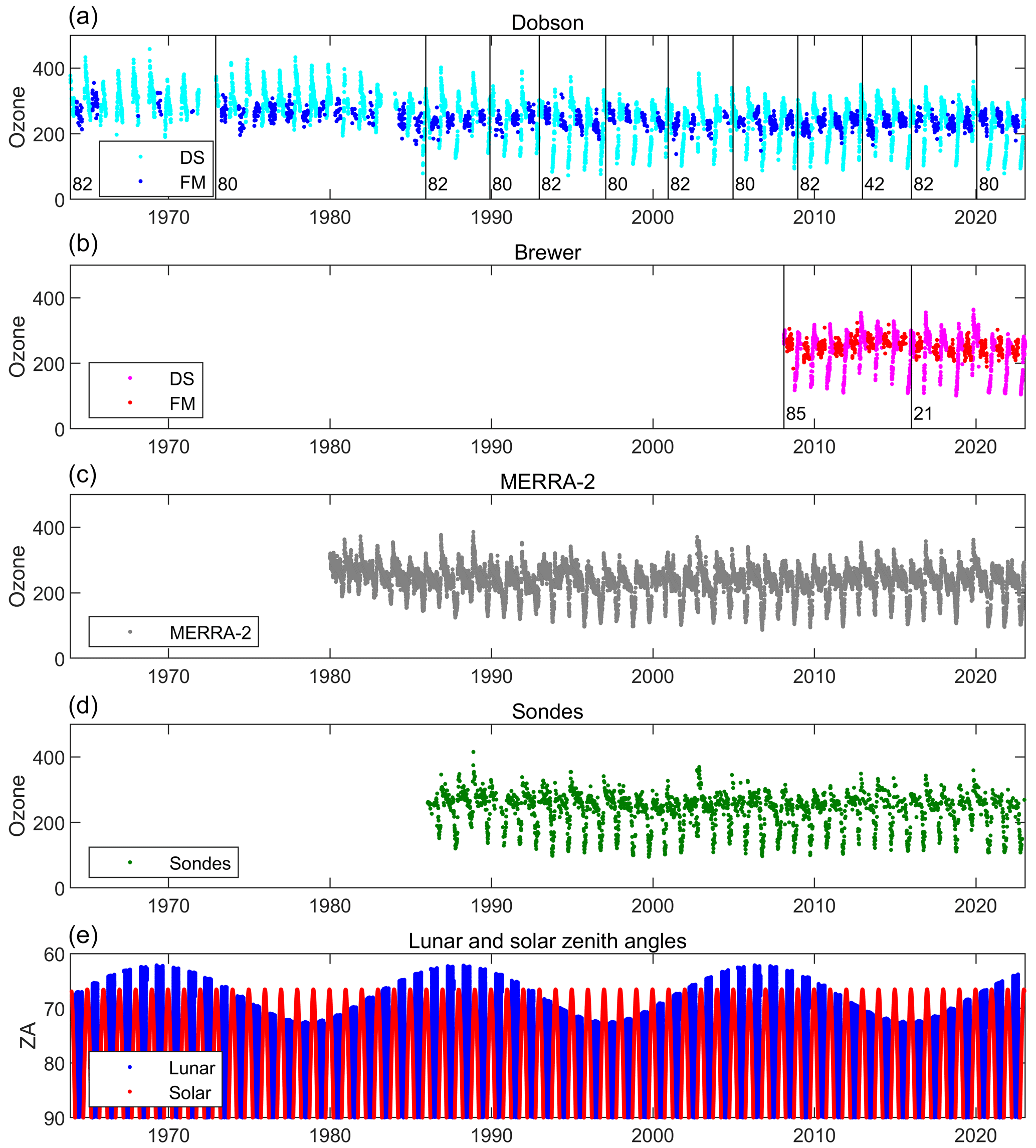
Figure 1(a–d) Total ozone time series from Dobson, Brewer, MERRA-2, and ozonesonde data for 1963–2022 as indicated in the plot. Each dot represents a daily mean value. The vertical lines correspond to Dobson and Brewer instrument changes. The instrument serial numbers are also shown. (e) The solar (red) and lunar (blue) zenith angles as a function of time. Note long-term variations of maximum lunar zenith angles between 63 and 73∘.
2.2 Brewer spectrophotometer, 2008–2022
The Brewer instrument was proposed by Alan Brewer (Brewer, 1973) and developed in the early 1980s at Environment and Climate Change Canada (ECCC) (Kerr, 2010; Kerr et al., 1981). Unlike the original Dobson instrument, it is a fully automated instrument that can take FM ozone measurements approximately every 15 min. More than 230 Brewer instruments have been manufactured, and 88 Brewer stations have reported their data to the WOUDC (Zhao et al., 2021) including 9 in Antarctica. ECCC Brewer no. 085 was installed, under an agreement between ECCC and the US National Oceanic and Atmospheric Administration (NOAA), in February 2008 (McElroy et al., 2010). It was replaced by ECCC Brewer no. 021 in December 2014 as shown in Fig. 1.
There are two main types of Brewer instruments. The originally developed instruments were single spectrophotometers (types Mark II and IV). The double monochromator (Mark III) was introduced in the early 1990s to reduce stray light and to enable accurate ozone measurements under low Sun conditions (Wardle et al., 1996), which is particularly important for high-latitude sites. The Mark III uses the same concept as the Mark II model but has a second spectrometer. Both Brewer instruments operated at the South Pole Station are Mark III type. All ECCC Brewers are calibrated against the Brewer world primary standard (the Brewer triad) at Toronto (Fioletov et al., 2005; Zhao et al., 2021). Although field Brewers are typically calibrated using traveling standards, Brewers 021 and 085, deployed to the South Pole Station, were calibrated against the triad Brewers in Toronto prior to their shipment to Antarctica.
The Brewer spectrophotometer is a modified Ebert grating spectrometer that measures the intensity of radiation at six selected channels in UV (303.2, 306.3, 310.1, 313.5, 316.8, and 320.1 nm); the four longer wavelengths are used to retrieve total column ozone. Similar to the Dobson instrument, the Brewer can perform ozone measurements in the DS, ZS, and FM modes. Details about the Brewer instrument, retrieval algorithm, instrument operation, and calibration can be found in an overview by Kerr (2010). Brewer data were processed by ECCC Brewer processing software (Siani et al., 2018) with all standard corrections (i.e., for the dead time, dark counts, and standard lamp tests) applied. Similar to the Dobson, the Brewer retrieval algorithm uses Bass and Paur ozone absorption cross-sections interpolated to a standard stratospheric temperature of −45 ∘C (Bass and Paur, 1985). Brewer ozone retrievals are much less affected by stratospheric temperatures than Dobsons (Kerr, 2002; Redondas et al., 2014; Gröbner et al., 2021). We estimated that the errors in retrieved ozone, introduced by the stratospheric temperatures over the South Pole, are under 0.4 %.
ECCC Brewers at the South Pole Station typically perform three to four FM measurements per hour during the polar night and five to six DS and ZS measurements per hour during the polar day. FM data were screened out if the standard error of individual measurements exceeded 12 DU (Dobson units), if the lunar disk illumination was less than 50 %, or if the lunar zenith angle exceeded 76∘. Brewer measurements at the South Pole Station are available from the WOUDC.
2.3 Ozonesondes, 1986–2022
Regular balloon-borne ozonesondes providing high-resolution vertical profiles of ozone and temperature at the South Pole Station started in 1986 (Hofmann et al., 1997, 2009; Solomon et al., 2005). There is typically one flight per week, although the frequency is often higher (two to three flights per week) during the ozone hole period. The electrochemical concentration cell (ECC) ozonesondes were used for the entire period, and their design (Komhyr, 1967) has remained relatively unchanged throughout the whole record. During the cold months (from April to mid-October), polyethylene film balloons were used to ensure burst altitudes of about 30 km. Standard rubber balloons were used for other months. The entire South Pole ozonesonde record has been harmonized by Sterling et al. (2018). An overall review of the record and estimates of ozone variability and trends for the ozone hole period are available from a recent paper by Johnson et al. (2023).
To obtain total ozone from an integrated ozonesonde profile, it is necessary to make assumptions about the ozone profile above the balloon burst height. There are two approaches developed for extrapolation of the ozone profile: (1) assuming a constant mixing ratio (CMR) of ozone above the balloon burst pressure (∼20 to 7 hPa) to zero pressure or (2) reconstructing the missing part of the profile using the satellite Solar Backscatter Ultraviolet Radiometer (SBUV) climatology (McPeters et al., 1997). Total ozone calculated by both methods is available from the datasets developed by NOAA. Following Wargan et al. (2017) and Johnson et al. (2023), the dataset used in this study is the one for which the interpolation is done by using the first method. As noted by Johnson et al. (2023), “the CMR extrapolation is more suitable over South Pole during the polar night and low Sun angle months when satellite and ground-based optical measurements are limited”. We have found that the differences in estimated total ozone long-term variation between the values estimated using the two methods are rather minor. Johnson et al. (2023) also reported that after the homogenization, there is a constant 2±3 % offset: ozonesonde total ozone is slightly higher than the DS Dobson observations.
2.4 MERRA-2 reanalysis data, 1980–2022
The second Modern-Era Retrospective analysis for Research and Applications (MERRA-2) is an atmospheric reanalysis from NASA's Global Modeling and Assimilation Office (Gelaro et al., 2017). MERRA-2 assimilates partial column ozone retrievals from the NOAA SBUV/2 series (nos. 11, 14, 16, 17, 18, 19) from 1980 to 2004. From October 2004, MERRA-2 has assimilated ozone profiles from the Microwave Limb Sounder (MLS) and total column data from and the Ozone Monitoring Instrument (OMI) (Wargan et al., 2017). Both OMI and MLS are on board the Earth Observing System Aura satellite that was launched in 2004. While SBUV and OMI measure ozone using solar light backscattered by the atmosphere, MLS observes thermal microwave emission from Earth's limb, and its stratospheric ozone mixing ratio data are available during the polar night up to 82∘ of latitude (Wargan et al., 2017); i.e., they cover a much larger area in winter compared to SBUV data that are available only for the sunlit atmosphere. Thus, the MERRA-2 ozone record was divided into two periods, herein referred to as the SBUV period and the Aura period. MERRA-2 total ozone is a continuous record from 1980 to 2022 with 1 h resolution. MERRA-2 ozone data have been found to have good quality when compared with satellite and ground-based observations (e.g., Rienecker et al., 2011; Wargan et al., 2017; Zhao et al., 2017, 2019, 2021). For example, in Zhao et al. (2021), the bias between Brewer world reference instruments and MERRA-2 is from −0.27 % to 1.05 % (hourly data; 1999–2019 period), with a monthly difference standard deviation less than 1.2 %.
Wargan et al. (2017) evaluated the MERRA-2 ozone fields using ground-based data including total ozone data from integrated ozonesonde profiles over the South Pole. They found that during both the SBUV and Aura periods, MERRA-2 is lower than the ozonesondes by 3 %, and the standard deviation of the difference between MERRA-2 and ozonesondes is 12 % in the SBUV period and only 5 % in the Aura period. Note that these numbers represent the estimates for the entire year, although Wargan et al. (2017) noted the existence of some systematic seasonal biases.
The time series of total ozone from the four data sources for the entire period of observations are shown in Fig. 1. The ozone hole formation is clearly visible in the plot, but it also shows that wintertime FM measurements by Dobsons and Brewers were taken almost every year, and a large number of such measurements are available. Note that while the solar zenith angles vary in the same range every year, the span of the lunar zenith angles is different from year to year (Fig. 1e) with the minimum value varying from about 62∘ to about 72∘. There are typically five to six periods during winter when the Moon is nearly full and the lunar zenith angles are the smallest (see Appendix A for details). As the range of lunar zenith angles slowly varies from year to year, artificial long-term changes in total ozone could be introduced if an instrument has a lunar-zenith-angle-dependent error.
To illustrate short-term ozone fluctuations and the measurement availability, Fig. 2 (top) shows total ozone values from the four data sources for 2 weeks in 2016 along with the lunar zenith angles and lunar disk illumination plots. While DS measurements at the South Pole Station are available almost every day in summer, the number of days with good-quality FM measurements per month is only four to seven (27 d of good FM nights per winter on average). In the example shown in Fig. 2 (top), there are two 4 d periods with continuous Brewer FM measurements when the Moon was nearly full, while Dobson data are available once a day, and ozonesonde data are available once a week. Although Brewer measurements show high scatter, both Brewer and MERRA-2 data demonstrate similar ozone fluctuations and the correlation coefficient between them is about 0.8. MERRA-2 data captured the rapid ozone changes on 20–22 June very well, although the peak on 16–17 July, which is seen in both Brewer and Dobson data, does not appear to the same extent in MERRA-2. Brewer measurements on 18–20 July show some diurnal variations that are not seen in MERRA-2. This could be related to some horizontal inhomogeneity of the ozone distribution over the pole that led to variations in ozone measured by Brewer due to a changing lunar azimuth angle. As Fig. 2 (middle and bottom) shows, the Dobson and Brewer measurements in the plot are taken during the optimal periods when the Moon was full, and the zenith angles were near the minimum.
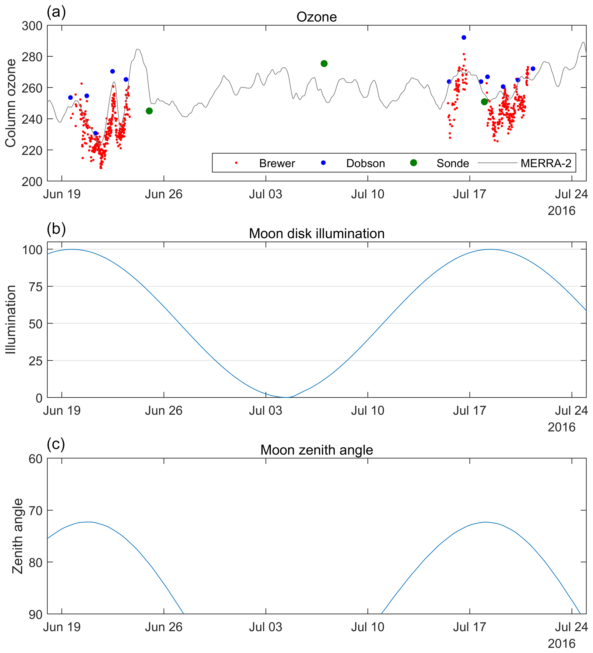
Figure 2(a) An example of wintertime ozone time series: total ozone from Dobson (the blue dots), Brewer (the red dots), ozonesonde (the large green dots), and MERRA-2 (the gray line) data for 18 June–24 July 2016. (b) The lunar disk illumination and (c) zenith angle for the same period.
MERRA-2 data can be matched with every Dobson, Brewer, and integrated total ozone measurement since 1980, and then differences with MERRA-2 can be used to analyze potential biases among the four datasets. Figure 3 (left column) shows the differences with MERRA-2 as a function of year and month of the year for the polar night (April–August) and polar day (October–February). March and September were excluded from the analysis since the number of Dobson and Brewer measurements during the sunrise and sunset months is very limited. It is expected that MERRA-2 total ozone would have different characteristics during the SBUV period (1980–2004) and the Aura period (2005–2022), and Fig. 3 shows the comparison results for these two periods separately.
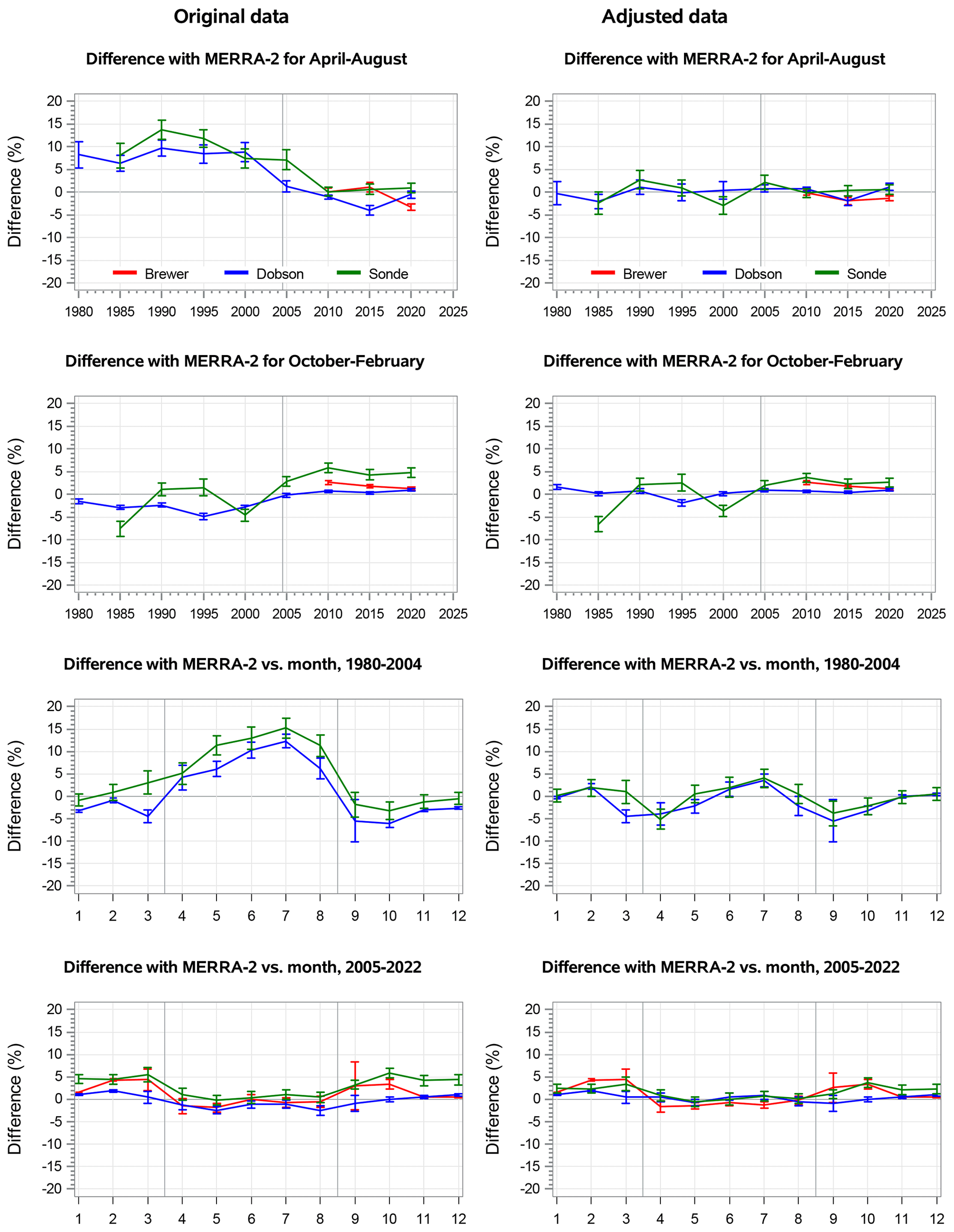
Figure 3Left panels: differences between MERRA-2 data and Dobson (blue), Brewer (red), and ozonesonde (green) total ozone in percent as a function of the year (two upper panels) and month of year (two bottom panels) for original data. Comparison was done for two seasons, April–August and October–February, and for two intervals: 1980–2004 and 2005–2022. Right panels: the same, but after adjustments were applied to MERRA-2, ozonesonde, and Brewer data. The vertical lines indicate the period from April to August. The error bars correspond to 2 standard errors of the mean.
There are several discrepancies between the four analyzed total ozone datasets during the wintertime. Some adjustments were applied to remove these discrepancies as described below. Dobson total ozone data were thoroughly analyzed (Bernhard et al., 2005) and corrected for known issues such as systematic errors related to the stratospheric temperature (Evans et al., 2017) in the past, and no further adjustments were applied in this study. However, three unrealistic Dobson FM ozone values below 200 DU in 2013, which were very different from the Brewer, ozonesonde, and MERRA-2 values, were deleted. As mentioned in Sect. 2.3, there is a 2 % bias (ozonesonde values are higher) between Dobson DS measurement and integrated ozonesonde total ozone (Johnson et al., 2023). The bias slightly depends on the analyzed time interval and season. We used a 2 % value for the bias, and all integrated total ozone values from ozonesonde flights were reduced by that amount.
MERRA-2 data during the SBUV period do not have any ozone measurements in the polar night area that can be used for data assimilation. Not surprisingly, there is a noticeable difference between the SBUV and Aura periods in wintertime MERRA-2 total ozone over the South Pole. There are two approaches to estimate that difference. First, Dobson data can be used as “true” values and the difference in ozone between the SBUV and Aura periods can be calculated from comparison with Dobson. Second, the switch from SBUV to Aura occurred in late 2004, i.e., near the maximum of stratospheric chlorine loading that occurred over Antarctica in 2000–2001 (Newman et al., 2007). Therefore, it can be expected that the ozone levels in the wintertime polar vortex remain approximately the same during a few years before and after the switch in 2004. Both these approaches give approximately the same differences, and based on these estimates, all April–August MERRA-2 data for 1980–2004 were increased by 8.5 % and data for 2005–2022 were decreased by 1.7 %. This correction removed a jump in the MERRA-2 record in 2004, and the 10-year averages prior to and after the switch in 2004 became nearly identical. The mean April–August values for 1995–2004 and 2005–2014 were equal to 245 DU from both Dobson and adjusted ozonesonde data. The same values were 225 and 250 DU for original MERRA-2, corresponding to 245 and 246 DU for corrected MERRA-2. There was also a 3 % mean difference between MERRA-2 and Dobson data in October–February 1980–2004. MERRA-2 data were adjusted to remove that bias. The mean difference between Dobson and MERRA-2 was less than 1 % during October–February 2005–2022, and no adjustment was applied to these data.
For Brewer DS measurements, there is good overall agreement with Dobson data, with a mean difference of 0.9 % and standard deviation of the difference for daily values of 4 %. There was also good agreement between Brewer 085 and 021 DS data during a 2-month period (December 2014–January 2015) when both instruments were at the South Pole Station: the mean difference was 0.4 % and the standard deviation of the difference was 0.5 %. For Brewer FM measurements, uncertainties and systematic errors are larger than for DS data. The mean Brewer–Dobson difference in April–August is 1.6 % and the standard deviation for daily values is 7.3 %. Thus, on average, independent Brewer FM measurements without any adjustments report total ozone values that are similar to those from the Dobson (within 1.6 %). There are, however, several sources of systematic errors in Brewer FM data that led to drifts in Brewer FM ozone values.
A detailed analysis of systematic errors of Brewers nos. 021 and 085 FM measurements is given in Appendix B. Both Brewers tend to overestimate ozone when lunar direct irradiance at 320 nm is low and when the lunar zenith angle is high. The overestimation is as large as 10 %–15 % when the ozone slant path is large (greater than 1000 DU). The latter leads to an artificial long-term change in wintertime total ozone due to long-term changes in the lunar zenith angle (Fig. 1). Corrections for these two factors were introduced, assuming that the data at the higher lunar irradiance and the lowest lunar zenith angles are accurate as discussed in Appendix B.
Figure 3 shows differences of Dobson, Brewer, and ozonesonde total ozone with MERRA-2 for the adjusted data (the right panel) for the same two periods and two seasons for the original data (left panel). The bias in MERRA-2 in April–August 1980–2004 is largely removed and ozonesonde data no longer show a difference with respect to the Dobson data. Figure 3 also shows that there is still some difference between adjusted MERRA-2 and Dobson data in individual winter months for the SBUV period. However, we applied a single correction instead of corrections for individual months for two main reasons. First, we preferred to change the data as little as possible to keep the data sources independent. Second, most of our results are related to wintertime averages. Since MERRA-2 data do not have any gaps, corrections for individual months would have the same impact on these averages as a single correction. In addition, the statistical uncertainty of a single correction factor is less than the uncertainty of correction factors for individual months. From now on, the adjusted data are used in this study, unless it is specifically stated otherwise. Note that these corrected Brewer data were also used in Fig. 2.
This study is focused on the period from April to August because the vortex is stable during that time and ozone is relatively unchanged, so its characteristics could be estimated from a limited number of measurements. This is further illustrated by Fig. 4 where the total ozone annual cycle for three periods is shown. The long-term monthly means in each of these 5 months are nearly identical. Only the August values were slightly lower in recent years because ozone depletion in the polar vortex starts in late August (e.g., Hassler et al., 2011). For this reason, data for 20–31 August were excluded from the analysis below. Figure 4 shows monthly mean values calculated from all available data for that month. Some differences between individual datasets in September–December are caused by the sampling bias. The number of Dobson and Brewer measurements in March and September is very limited, and the measurements are not available in the second half of September. Ozonesonde flights were more frequent when the ozone hole was over the South Pole. There is no sampling bias in April–August, although MERRA-2 data were available every day, while ozonesonde are flown four to five times a month and Dobson and Brewer measurements were taken 5–7 d per month.
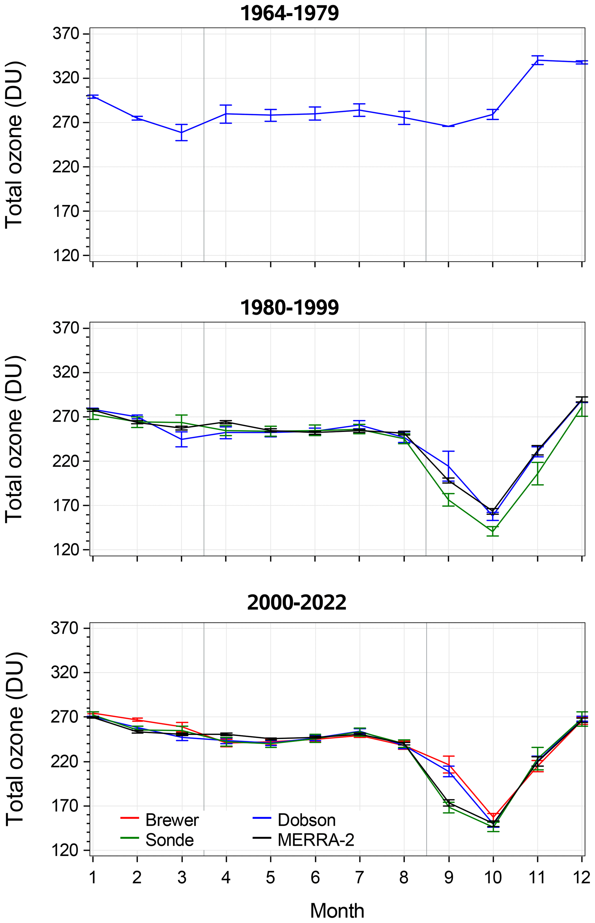
Figure 4Total ozone annual cycle from Dobson (blue), Brewer (red), ozonesonde (green), and MERRA-2 reanalysis (black) data for three intervals as indicated in the plot. The vertical lines indicate the period of stable ozone in the vortex from April to August. The error bars correspond to 2 standard errors of the mean. The differences in September–December are caused by the sampling bias: the number of Dobson and Brewer measurements in March and September is very limited, and they are missing in the second half of September. Ozonesonde flights were more frequent when the ozone hole was over the South Pole. Note that there is no sampling bias in April–August.
It is challenging to make Dobson and Brewer measurements during the polar night, and such measurements are subject to considerable uncertainties. Nevertheless, the correlation coefficients in April–August between MERRA-2 daily means and Dobson, Brewer, and ozonesonde total ozone daily values were all about 0.8 during the Aura period (2005–2022). The correlation coefficient between Brewer and Dobson measurements is slightly lower at about 0.7, suggesting that there is some noise in these measurements. For the MERRA-2 SBUV period (1980–2004), the correlation with Dobson and ozonesonde data was much lower: only about 0 4. The correlation coefficient between ozonesonde and Dobson values for 1986–2004 was 0.55 compared to 0.83 for 2005–2022, suggesting that Dobson and/or ozonesonde data were also less accurate during the first period.
The correlation coefficient is not the appropriate characteristic to describe uncertainties of individual data sources since it also depends on the variability of ozone itself, which is low in the wintertime polar vortex. As total ozone data from several sources are available, information on the instrument uncertainties and ozone variability can be derived by comparing data from individual sources (Grubbs, 1948; Fioletov et al., 2006; Toohey and Strong, 2007; Zhao et al., 2016): a measurement result (M) is the sum of the true value (X) and an error (e). Supposedly, the two instruments measure the same parameter X, but with different errors e1 and e2. If we assume that the measured value and the errors are independent and the errors of different instruments are not correlated, then the results of their measurements (M1 and M2) can be used to estimate the variance of X, e1 and e2:
The equations above can be used to estimate the standard deviation of instrument errors (or instrument uncertainty) and the standard deviation of ozone variability from pairs of coincident Dobson, Brewer, and MERRA-2 data points (ozonesonde data are too sparse). The results for daily and monthly values are shown in Table 1. The values are given for two periods that correspond to the two MERRA-2 data sources (SBUV and Aura). The 1980–1984 interval of rapid ozone changes was excluded from the calculations.
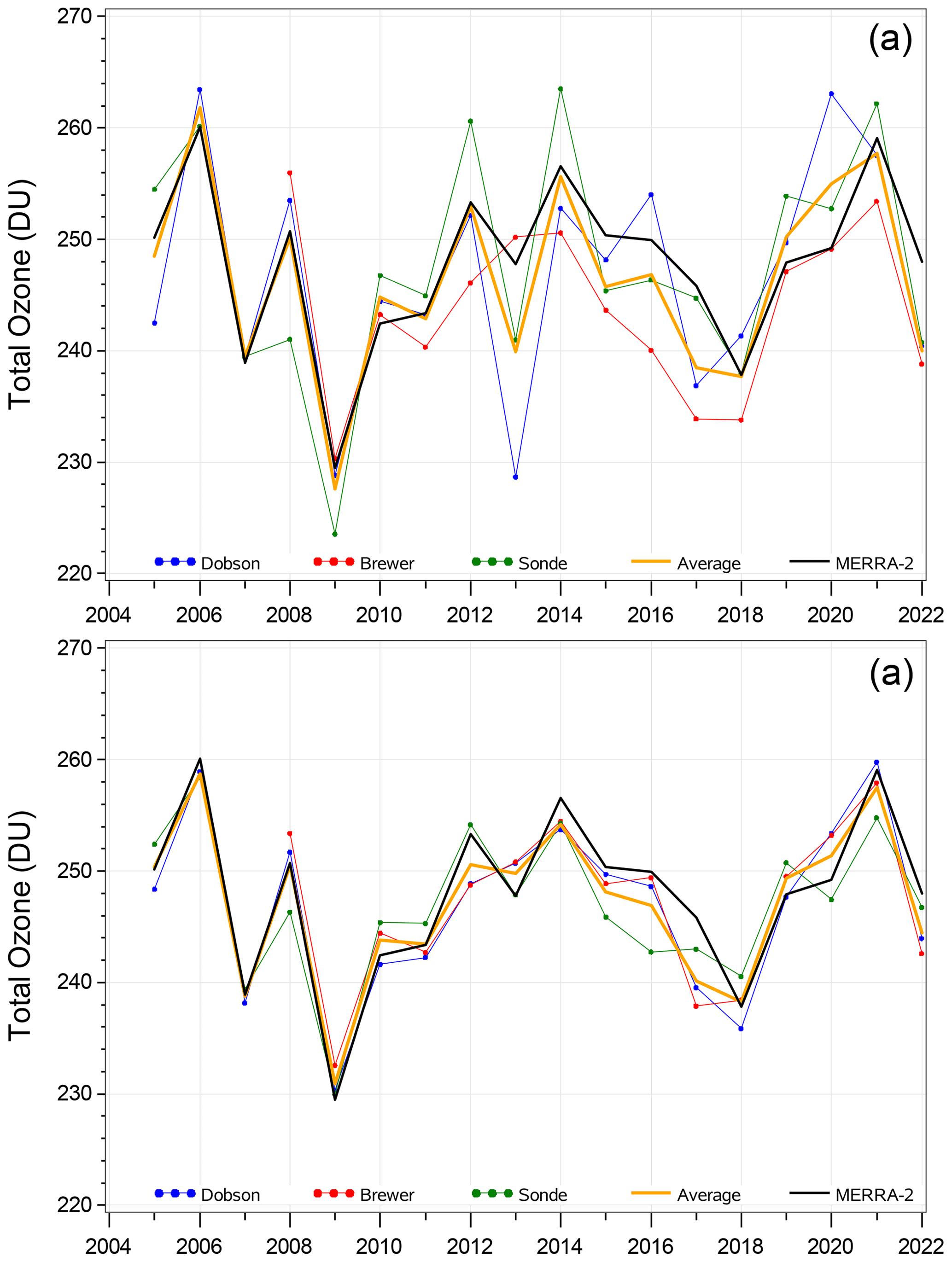
Figure 5(a) Mean wintertime ozone for 2005-2022 from Dobson (blue) and Brewer (red) daily values, ozonesonde (green) total ozone, and MERRA-2 reanalysis (black). The average of Dobson, Brewer, and ozonesonde data is shown by the orange line. (b) The same as above, but with MERRA-2 data coincident with Brewer and Dobson observations and ozonesonde flights used instead of the actual measurements. Note that the pre-1980s level is 280 DU.
Table 1Standard deviation for monthly and daily values, estimated uncertainties, and total ozone variability (DU).
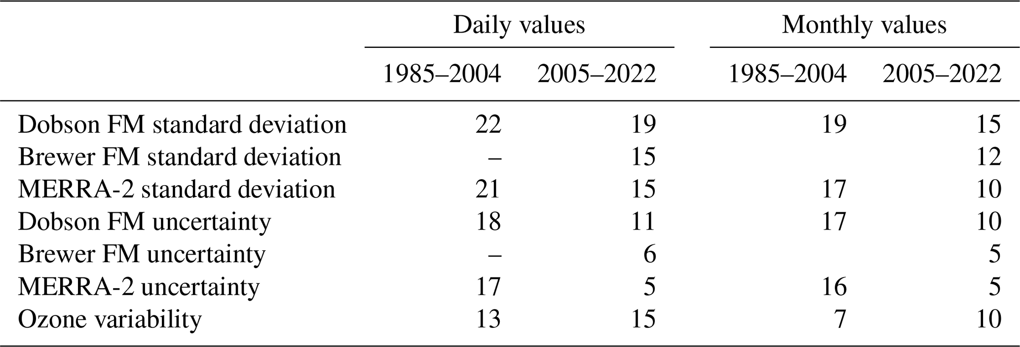
The uncertainties are estimated from two pairs of data sources; e.g., the Dobson uncertainty can be estimated from the Dobson–Brewer and Dobson–MERRA-2 pairs, and their average is shown in the table. The ozone variability can be estimated from three pairs, and their average given in the table.
The MERRA-2 uncertainties are lower in 2005–2022 than for the first period, suggesting that the addition of MLS data improved the reanalysis. The uncertainties in Dobson data appear to be larger than those for Brewer and MERRA-2, but this is because we compared daily averages. Unlike the Brewer and MERRA-2 that provided multiple measurements throughout the day, the Dobsons provided only one value. The uncertainties of Dobson and Brewer daily mean FM values are 6–11 DU or about 2.5 %–4 %. The estimated wintertime ozone variability is relatively low at about 15 DU for daily averages and 10 DU for monthly values, or about 6 % and 4 %, respectively. Therefore, the wintertime total ozone levels can be established from a relatively limited number of measurements.
Statistics of mean wintertime total ozone (i.e., one value per year calculated as an average of all wintertime data in that year) are available in Table 2. The values are given in Dobson units (DU) for the two time intervals discussed above (i.e., 1985–2004 and 2005–2022). Figure 5 (top) shows the time series of wintertime total ozone values for 2005–2022, i.e., for the period of the most accurate ozone values (note that MERRA-2 adjusted data were used, although the adjustment for that period was only 1.7 % as mentioned above). Individual datasets capture the main features of year-to-year variability in wintertime ozone, although there are some differences likely caused by instrumental issues. The correlation coefficients between Dobson, Brewer, and ozonesonde values and MERRA-2 were in the range from 0.74 to 0.85. The correlation of their average with MERRA-2 is even higher at 0.9, as instrumental noise and sampling issues are partially canceled out. The standard deviation of the difference between MERRA-2 and Dobson, Brewer, and ozonesonde wintertime values is between 5 and 7 DU (2 %–3 %). It is even lower (3.7 DU) for the difference between MERRA-2 and the average of the Dobson, Brewer, and ozonesonde wintertime values.
Table 2Statistics of the mean wintertime ozone for 1985–2004 and 2005–2022 in Dobson units (DU).
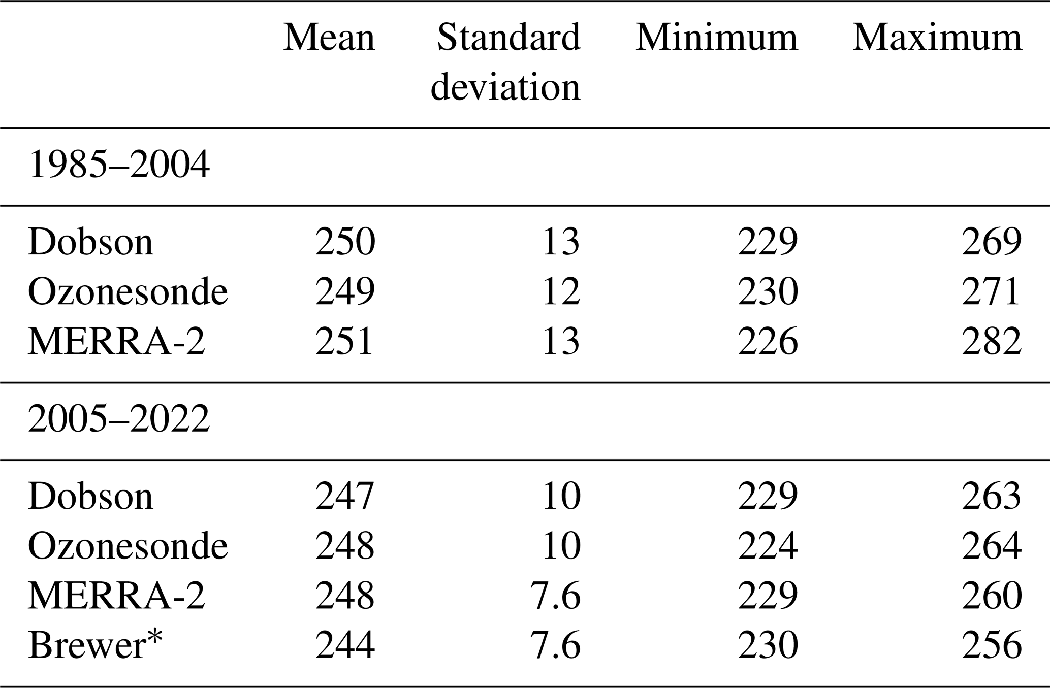
* Brewer data are available only for the period 2008–2022.
As mentioned, the number of Dobson, Brewer, and ozonesonde measurements is very limited in the wintertime. To illustrate the sampling issues, Fig. 5 (bottom) shows time series of MERRA-2 data for the same period taken at the time of Dobson, Brewer, and ozonesonde measurements as well as the complete MERRA-2 record. In other words, MERRA-2 data were resampled at the time of the actual Dobson, Brewer, and ozonesonde measurements and then compared with a complete MERRA-2 record. Although the Dobson, Brewer, and ozonesonde measurements are available only for 15 %–20 % of all days in April–August, MERRA-2 data sampled on days and at times of their measurements can successfully reproduce mean wintertime values calculated from the continuous MERRA-2 record. The standard deviation between them is only 2.5–3.5 DU (1 %–1.5 %), while the average of all these sampled data has a standard deviation from the complete MERRA-2 record of only 2.2 DU (∼0.9 %).
4.1 Time series
There were a total of 258 daily FM measurements by Dobsons nos. 80 and 82 in April–August in 1964–1980. The average of these measurements is 280±3.2 DU (2σ level), which can be used as a benchmark for the pre-1980s ozone, and then the deviation from that level can be estimated. Figure 6 (top) shows the deviations from this pre-1980 level for Dobson, Brewer, ozonesonde, and MERRA-2 total ozone. Each symbol in the plot represents a 5-year average. There is a clear decline from the pre-1980s level, and the ozone values were about 12 % below that level after the mid-1980s. As discussed above, the differences between individual datasets are 2 %–3 %, so such large deviations can be reliably measured by several independent datasets. Moreover, the MERRA-2 record started in 1980 and the deviation from the 1980 level and the values in 2000 is about 12 %. So, a 12 % decline can be seen independently from both the Dobson record and MERRA-2 total ozone (the SBUV period).
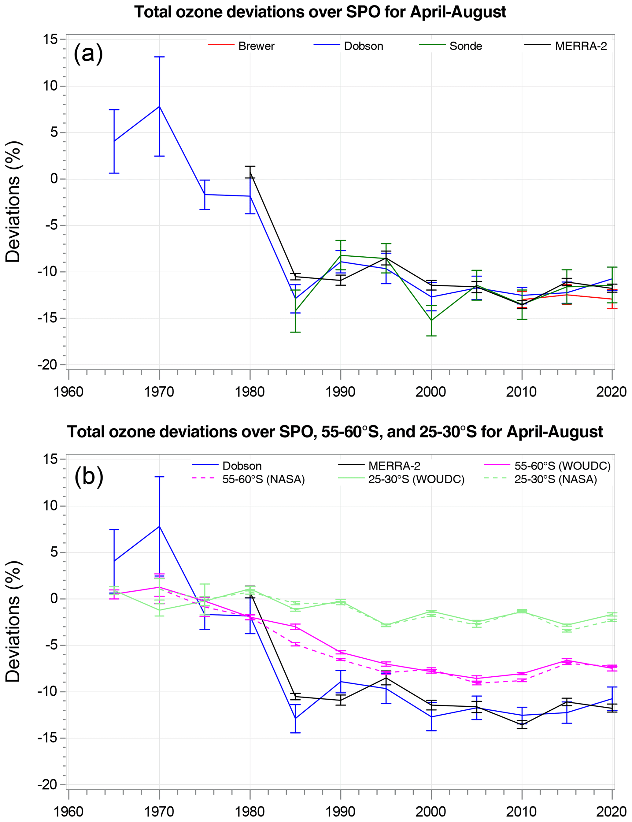
Figure 6Mean total ozone deviations from the pre-1980 level for April–August in percent. (a) Deviations over the South Pole based on Dobson (blue) and Brewer (red) FM measurements, integrated ozonesonde profiles (green), and MERRA-2 reanalysis (black) data. Data were adjusted as discussed in the text. (b) Deviations over the pole from Dobson and MERRA-2 data (the same as in the top panel) as well as ozone deviation from the pre-1980 level over 25–30∘ S (magenta) and 50–60∘ S (green) estimated from NASA merged satellite dataset (dashed lines) and WOUDC ground-based dataset (solid lines). Each symbol represents a 5-year average, and the error bars correspond to 2 standard errors of the mean.
The year-to-year variability of wintertime polar ozone (Table 2) in recent years is relatively small compared to that 12 % decline. The standard deviations of the wintertime values are only 3 %–4 % for 2005–2022, so a 12 % decline corresponds to 3 to 4 standard deviations. Moreover, the maximum values over that period from all four data sources were at least 16 DU (or more than 6 %) below the benchmark value of 280 DU.
This observed 12 % decline of wintertime polar ozone is much larger than a long-term decline from the pre-1980s levels over southern middle and high latitudes, where the decline is about 5 % (e.g., Weber et al., 2022; WMO, 2022). This is further illustrated in Fig. 6 (bottom), which shows wintertime deviations from the pre-1980 level over low and high southern latitudes from two independent datasets of zonal mean values: the WOUDC ground-based dataset (Fioletov et al., 2002) and the merged SBUV dataset (Frith et al., 2014). It is not unexpected because the trend estimates for the Southern Hemisphere for the period from the late 1970s to the late 1990s show an increase in the negative trend magnitude going toward the pole (e.g., Fioletov et al., 2002; Vyushin et al., 2007; Weber et al., 2022). The wintertime long-term decline over the South Pole is probably the largest long-term ozone decline aside from the springtime Antarctic ozone depletion.
Figure 7 (the left panel) shows seasonal mean total ozone over the South Pole for three seasons (January–February, April–August, and October–December) from the four data sources. The October–December ozone shows the largest decline, but the year-to-year variability is also the largest due to the variability of the extent and duration of the ozone hole. The interpretation of these data clearly requires additional proxies (e.g., de Laat et al., 2015). January–February data show a smaller decline and smaller variability than the data in October–December. In October–February, SBUV and OMI total ozone is available for MERRA-2 data assimilation and Dobson and Brewer can take the most accurate DS measurements, so the agreement between the different datasets is very good (as discussed in Sect. 3). Section 3 also demonstrates that the correlation between Dobson and MERRA-2 data is not very high in April–August during the MERRA-2 SBUV period, and this can also be seen in Fig. 7. The agreement between the four datasets in April–August has become much better after 2005, i.e., when MERRA-2 started to use MLS data.
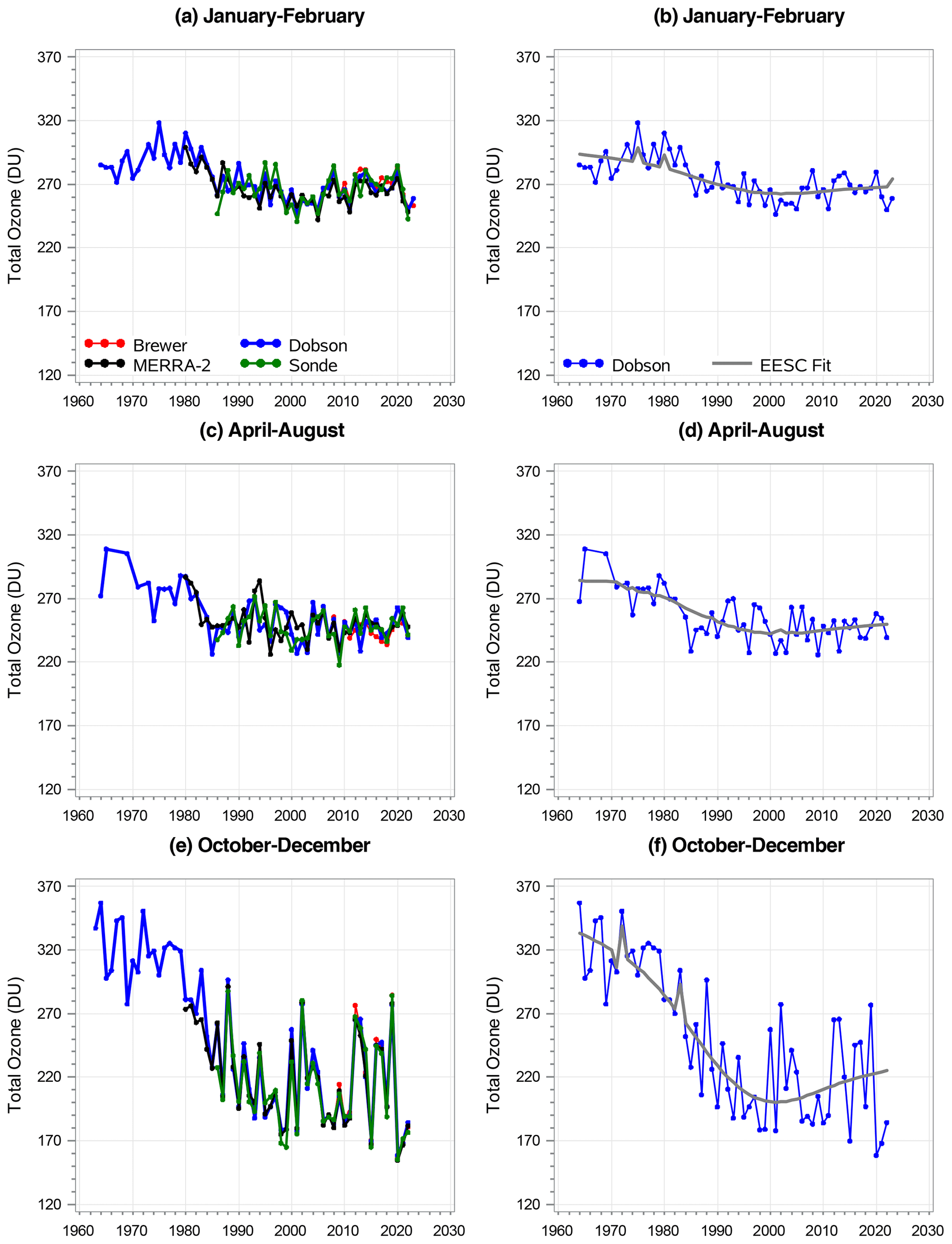
Figure 7(a, c, e) Seasonal mean total ozone over the South Pole from Dobson (blue) and Brewer (red) FM measurements, integrated ozonesonde profiles (green), and MERRA-2 reanalysis (black) data for three seasons as indicated in the plot. (b, d, f) Dobson seasonal mean ozone (blue) and the fit (gray) of Dobson data by the equivalent effective stratospheric chlorine (EESC) curve. Fitting was done separately for each month, and then the fitting results were averaged based on Dobson data availability to form the seasonal means.
4.2 The EESC fit
The long-term ozone decline is caused by an increase in ozone-depleting substances (ODSs) in the stratosphere (WMO, 2018, 2022). The ODS concentration is often described by equivalent effective stratospheric chlorine (EESC) (Newman et al., 2007). It is a function that exponentially increased during the 1960s and 1970s, leveled off in the late 1990s-early 2000s, and slowly declined thereafter. EESC also slightly depends on latitude and altitude. EESC is used as a proxy for long-term changes in total ozone (e.g., Fioletov and Shepherd, 2005; Stolarski et al., 2006; Wohltmann et al., 2007; Vyushin et al., 2007; de Laat et al., 2015). Although the results of the EECS-based estimates for the ozone recovery trend assessment should be interpreted with caution (Kuttippurath et al., 2015), we can use them to verify how well the EESC curve describes the observed long-term ozone changes. For EESC we used a version with an age of air of 5.5 years, age of air spectrum width of 2.6 years, and Bromine scaling factor of 60 that corresponds to the polar stratosphere (Newman et al., 2007). The fitting results of Dobson data by the EESC function for the three seasons are shown in Fig. 7 (the right column). Fitting was done separately for each month, and then the fitting results were averaged based on Dobson data availability to form the seasonal means:
where Xi(m,y) is total ozone observation with number i in month m and year y, EESC(m, y) is the EESC value for month m of year y, εi(m,y) represents the residuals, and am and bm are unknown coefficients for month m. The coefficients am and bm were estimated for each month of the year by the least square method. Then, the seasonal means of the fitting results (F(y)) were calculated for every winter (i.e., for months 4 to 8) as
where n(my) is the number of Dobson measurements in month m of year y. As Fig. 7 (middle) shows, the fitted curve followed April–August Dobson values well.
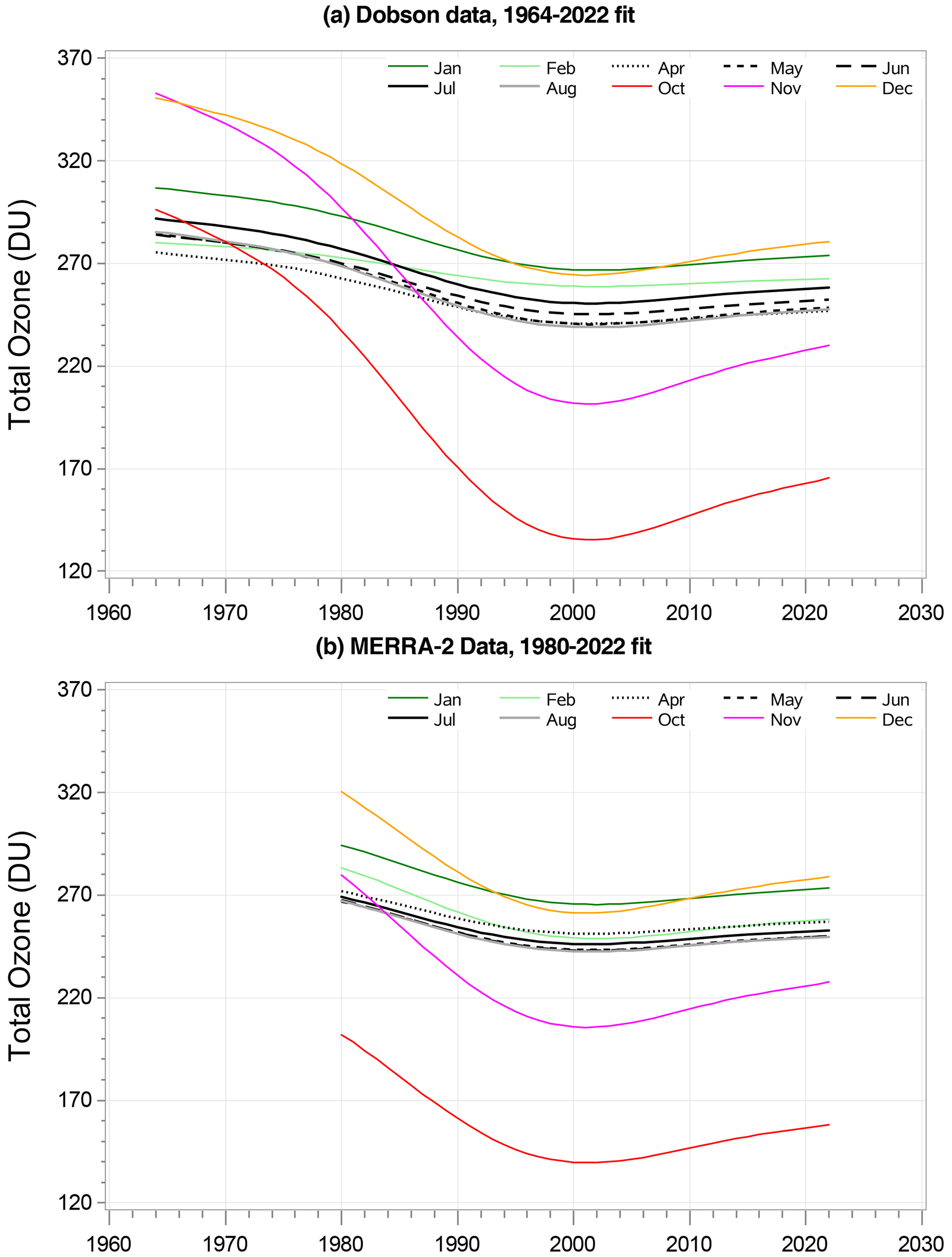
Figure 8(a) Fits of Dobson data in different months (as indicated in the plot) by the EESC curve using 1964–2022 data. (b) The same, but for MERRA-2 data for 1980–2022. Although fitting was done individually for each month, the differences between April and August EESC curves (black and gray) are within 10–15 DU, suggesting that long-term changes in the polar vortex total ozone are uniform for all wintertime months. Note that in August, only the first 20 d were used for the fit.
The main advantage of studying long-term changes in wintertime ozone is that, unlike all other months, the long-term changes in April–August are very uniform. This can be illustrated by the EECS fits. Figure 8 shows the fitting results of Dobson (Fig. 8, top) and MERRA-2 (Fig. 8, bottom) data with the values for each month fitted separately. The fitting results for April–August are very similar (and different from the fitting results for all other months). This similarity means that the April–August data can be lumped together for long-term change studies. It should be mentioned that if data for 21–31 August were included into the August record, the fitting curve for August would noticeably deviate from the April–July fitting curves.
Table 3Total ozone values (in DU) in 1964, 1980, 2001, and 2022 estimated from the EESC fit for Dobson and MERRA-2 data. The overall decline in 2022 from the 1964 level and the pre-1980s values as well as the ratio of the EESC-related fitting parameter to its standard deviation are shown.
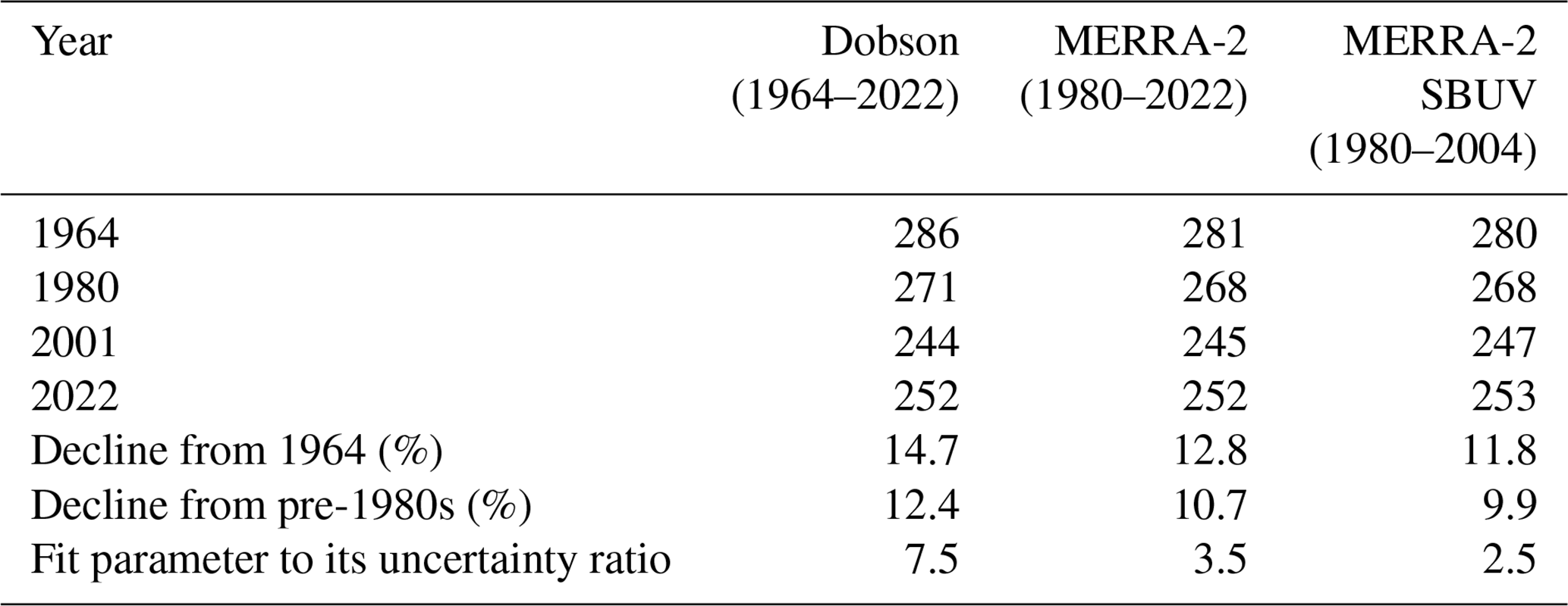
As the next step, the average of all data for the period from 1 April to 20 August of each year was calculated as was the wintertime total ozone using the EESC curve. The results are shown in Table 3 in the form of ozone values in different years, estimated from the fit. Dobson and MERRA-2 data show a decline from the pre-1980s level to 2001 (the maximum of the polar EESC curve) of 12 % and 11 %, respectively, i.e., similar to what was seen in the deviation plot (Fig. 6). There is an additional decline of about 2 % from 1964 to 1980.
It is interesting to note that the April–August fitting results for Dobson data and MERRA-2 are very similar, although the first 15 years of the Dobson record are not available from MERRA-2. Moreover, the EESC fit is not very different even if we estimate it from the MERRA-2 SBUV period only (i.e., limit the data to 1980–2004). The decline from the pre-1980s level is about 10 %. This can be used as an argument that long-term wintertime ozone changes indeed follow the EESC curve. The uncertainties of the EESC fit are given in the bottom line of Table 3 as the ratio between the parameter of the EESC fit to its standard deviation. For the Dobson record, the ratio is 7.5, so the decline from the pre-1980s has a 2σ uncertainty of 3.3 %, and therefore the differences in estimated declines for 1964–2022 from Dobson data and for 1980–2004 from MERRA-2 data are within the uncertainty. The uncertainties of MERRA-2-based estimates are larger (the ratios are smaller) due to a shorter time interval.
Table 4The ozone recovery trends and their standard deviations (in brackets) for 2001–2022 and 2005–2022 from different data sources. The values are given in percent per decade and as a total change in percent.
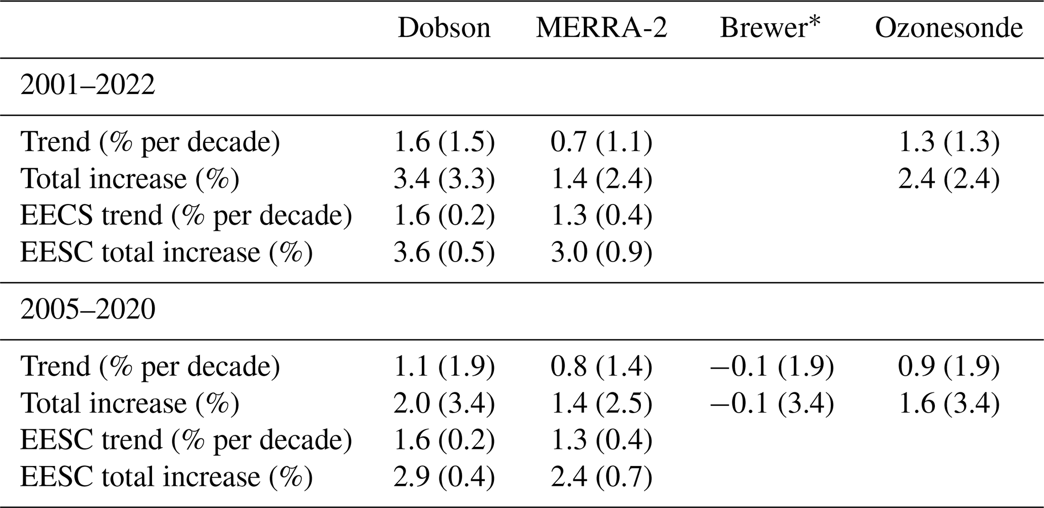
* Brewer data are available only for the period 2008–2022.
4.3 On ozone recovery in the wintertime
Detection of ozone recovery is an important current research topic (e.g., Steinbrecht et al., 2018; Weber et al., 2022). From the EESC changes, it is expected that the magnitude of positive recovery trends are only one-third of the magnitude of the magnitude of negative ozone decline trends. Large natural ozone variability makes the detection of such a small rate of recovery complicated. In addition, the total ozone recovery may be also inhibited by ozone decline in the lower stratosphere (Ball et al., 2018). The South Pole wintertime total ozone record was examined to detect the recovery in two ways: from the EESC fit and as a linear trend in the wintertime values. The results are summarized in Table 4 for two time intervals. The 2001–2022 interval corresponds to the declining part of the EESC curve, while the 2005–2022 interval corresponds to the Aura part of MERRA-2. From the EESC fit, the increase is 1.3 %–1.6 % per decade. Dobson and ozonesonde data for 2001–2022 show similar values of the linear trend, although the trend 1σ uncertainties are as large as the trend itself. However, the MERRA-2 trend is nearly half that of the Dobsons and ozonesondes, probably due to a lower quality of MERRA-2 data from the SBUV period. For the 2005–2022 period, data from Dobsons, ozonesondes, and MERRA-2 show a similar decline, but the magnitude of that trend is smaller than that for 2001–2022. The trend from Brewer data is almost zero, but it cannot be compared with the mentioned Dobson and ozonesonde trends since the Brewer record started only in 2008.
These trend uncertainty estimates reflect large ozone fluctuations shown in Fig. 5. They are likely caused by dynamical factors related to the formation and strength of the polar vortex. Therefore, the uncertainties can be reduced by adding proxies that are related to these factors. However, such analysis is outside the scope of this study.
The Antarctic polar vortex creates unique chemical and dynamic conditions when the stratospheric air over Antarctica is isolated from the rest of the stratosphere. The vortex is formed in late autumn, and it typically breaks up in October–December. The sunrise and extremely cold temperatures create favorable conditions for rapid ozone loss after sunrise; however, for a 5-month period from April until late August, stratospheric ozone within the vortex remains largely unchanged. Such prolonged stable conditions within the vortex make it possible to estimate the total ozone levels there from sparse wintertime ozone observations at the South Pole.
The available records of focused Moon (FM) observations by Dobson and Brewer spectrophotometers at the South Pole Station (for the periods 1964–2022 and 2008–2022, respectively) as well as integrated ozonesonde profiles (1986–2022) and MERRA-2 reanalysis data (1980–2022) were used to estimate the total ozone variability and long-term changes. Some adjustments were applied to the original data to make the data records consistent. No adjustment was applied to the Dobson record, and only three unrealistic values were removed in 2013. Ozonesonde data were decreased by 2 % to match the Dobson values. MERRA-2 data have about 10 % systematic bias between the wintertime values during the SBUV period (1980–2004) and the OMI/MLS period (2005–2022). To remove this bias and make the data consistent with the Dobson record, wintertime MERRA-2 data for 1980–2004 were increased by 8.5 % and data for 2005–2022 were decreased by 1.7 %.
While Dobsons typically report only one measurement per day, Brewers provide a nearly continuous record of total ozone measurements when the Moon is full and lunar zenith angles are small enough. In general, Brewers report an average wintertime total ozone level that is similar to that from the Dobson. There is, however, a major issue with Brewer FM data: they overestimate ozone by 10 %–15 % when the slant path is high (greater than 1000 DU). This is likely related to the instrument's performance when the lunar radiation is low.
Although Dobson, Brewer, and ozonesonde measurements are sparse, they can be used to accurately estimate wintertime ozone. The sampling effect was estimated by comparing wintertime ozone values calculated from continuous MERRA-2 data with MERRA-2 data sampled only at the time of Dobson, Brewer, and ozonesonde measurements. This comparison demonstrated that the wintertime values can be estimated from such MERRA-2 resampled data with a standard deviation of 2.5–3.5 DU (or 1 %–1.5 %), while the average of all these resampled data has a standard deviation from the complete MERRA-2 record of only 2.2 DU (∼0.9 %).
The wintertime ozone variability over the South Pole is low. The estimated standard deviation of the ozone variability is 13–15 DU for daily values and 7–10 DU for monthly means. The standard deviation of annual mean wintertime ozone is about 10 DU, although this number is inflated because it includes some instrumental errors. This number is small compared to the 30 DU (11 %–12 %) ozone decline from the average of about 280 DU prior to 1980 and the present level of about 250 DU.
The wintertime total ozone variations over the South Pole support the statement that the changes that are expected agree with the shape of the EESC curve. From the EESC fit, the decline from the pre-1980s level to 2001 (the maximum of the polar EESC curve) is about 12 %. There is an additional decline of about 2 % from 1964 to 1980. From the EESC fit, the expected ozone increase rate after 2001 is 1.3 %–1.6 % per decade. Although the variability in wintertime ozone is not very high, it is still difficult to find a statistically significant positive ozone recovery trend. Dobson and ozonesonde data demonstrate a 1.3 %–1.6 % positive trend for the period of the EESC curve maximum (2001–2022), but the 1σ trend uncertainties are as large as the trend itself. MERRA-2 data for the same period show only half of the observed trend, perhaps because of large uncertainties during the MERRA-2 SBUV period.
Wintertime polar ozone is affected by all the factors contributing to the changes in the ozone layer, probably to the largest extent. The contribution from dynamic factors to ozone variations in the polar region is probably similar to that anywhere else in the southern middle and high latitudes. A decline in ozone due to gas-phase ozone destruction from ODSs is probably the largest, since the time for an air parcel to travel from the tropics to high latitudes due to the Brewer–Dobson circulation in austral spring–summer is the longest. As a result, the decline in wintertime polar ozone is probably the largest long-term ozone decrease aside from the springtime Antarctic ozone depletion. Possible changes in the Brewer–Dobson circulation in the Southern Hemisphere would also likely have a larger impact over the South Pole than over the lower latitudes. The wintertime ozone values over the South Pole during the last 20 years were about 12 % below the pre-1980s level; i.e., the decline there was nearly twice that over southern midlatitudes. Thus, wintertime ozone values in the polar vortex can be used as an indicator to diagnose the state of the ozone layer. It is also important to stress that such diagnostics require data only from one station.
The combination of the Earth's rotation and the Moon's rotation around the Earth creates a peculiar pattern of the lunar disk illumination and lunar zenith angle distribution as shown in Fig. A1 for 2 years. Figure A2 shows the solar and lunar zenith angles for the periods of high and low Moon elevation above the horizon. Since only conditions with the Moon disk illumination greater than 50 % and zenith angles less than 76∘ for Brewer and ∼80∘ for Dobson are suitable for measurements, there are only five to six short periods per winter when such measurements can be performed.
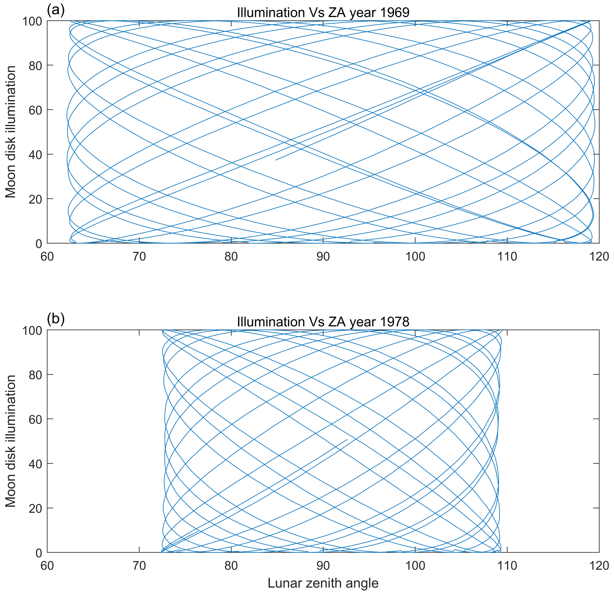
Figure A1The distribution of the lunar disk illumination and lunar zenith angle values in (a) 1969 and (b) 1978.
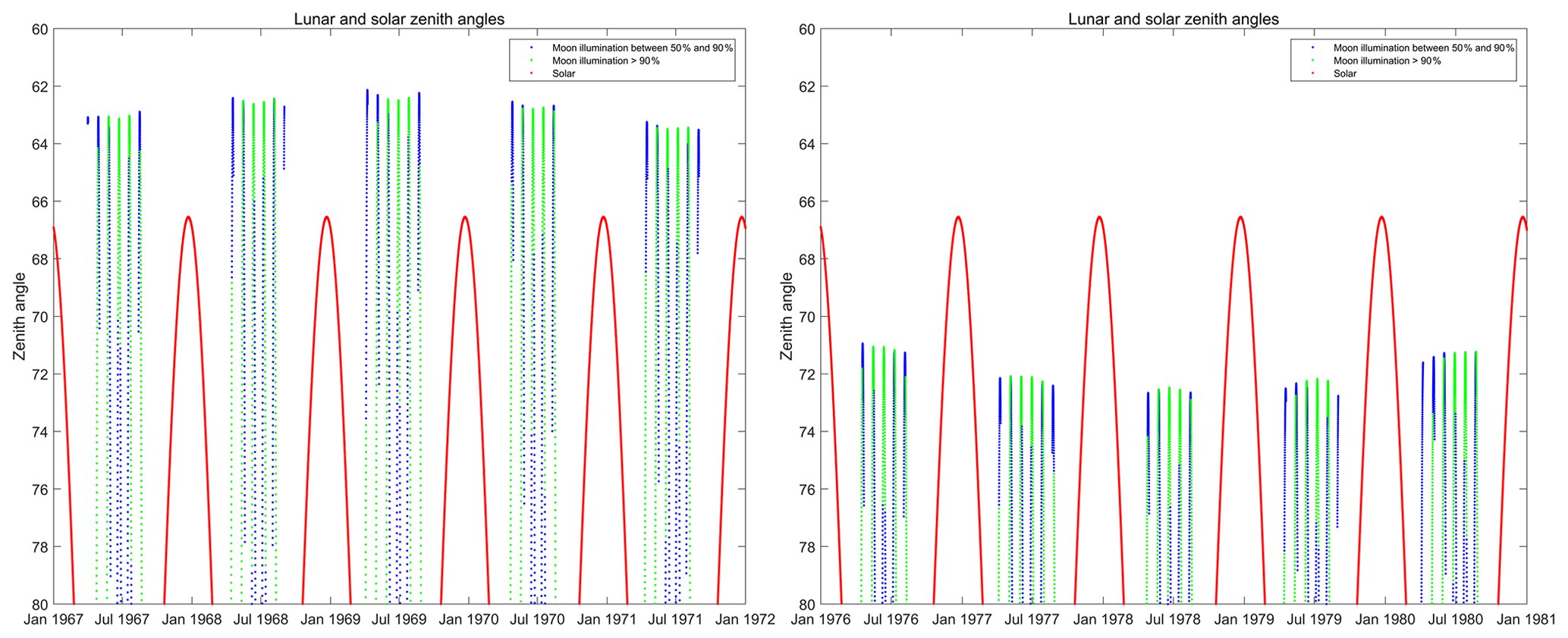
Figure A2Plot of the solar (red) and lunar zenith angle (green and blue) as a function of time for two time intervals (and 1967–1971 and 1976–1980) that correspond to periods of high and low Moon elevation above the horizon. Each dot corresponds to 1 h. Blue dots correspond to the lunar disk illuminations between 50 % and 90 %, and green dots correspond to the lunar disk illumination above 90 %.
We found that Brewer measurements overestimate ozone when the lunar radiation intensity is low. “Signal 320”, i.e., the natural logarithm of the number of photon counts per second at Brewer slit 5 (approximately 320 nm), adjusted for the dead time, the number of “dark” counts, and instrument temperature response (Kerr, 2010) were used here to assess the lunar radiation intensity. Figure B1 shows the difference between Brewer and MERRA-2 ozone data as a function of Signal 320. For low lunar radiation intensity, Brewer ozone values are higher than MERRA-2 by 10 %–15 % for Brewer no. 085 and by 5 %–10 % for Brewer no. 21, although both instruments show near-zero differences for Signal 320 equal to 11. Such dependence of the difference on the Moon's radiation intensity is probably related to nonlinearity of the Brewer photomultiplier sensitivity at low signals. The 320 nm wavelength is the longest used in the Brewer FM and DS ozone retrieval algorithms (besides the three other shorter wavelengths), and the ozone absorption is low at that wavelength. Therefore, Signal 320 is practically not affected by the ozone slant column, and all ozone measurements can be grouped by Signal 320.
Comparison with MERRA-2 was used to evaluate possible biases in Brewer data since MERRA-2 does not depend on lunar radiation. Figure B2 shows the difference between Brewer and MERRA-2 total ozone as a function of the slant column for the values of Signal 320 between 9 and 10.5 (the left column) and above 10.5 (the right column). A similar plot for the Dobson measurements is also shown. The slope is increasing with a decline in Signal 320. We removed all data for Signal 320 less than 9 because the faction of such measurements is small and the bias in ozone values is large. The data with Signal 320 greater than 10.5 show some dependence of the difference on the slant column, but most such data correspond to slant columns under 800 where the difference is small. However, if we just discard all data with Signal 320 less than 10.5, the number of days with FM measurements is reduced by 50 % for Brewer 21 and by 80 % for Brewer 85. For this reason, we applied an empirical correction () to remove a linear trend in the difference with MERRA-2 as a function of the slant column if Signal 320 is between 9 and 10.5. This correction has completely removed the dependence of the difference on Signal 320 for Brewer no. 021, but not for Brewer no. 085. As Fig. B1 shows, the lunar radiation dependence effect was larger for Brewer no. 85 than for Brewer no. 21, while the suggested correction was the same for both Brewers. We applied another correction for Brewer no. 085 that was 0 for Signal 320 greater than 10.5 and linearly decreased from 0 % to −4 % for Signal 320 declining from 10.5 to 9.
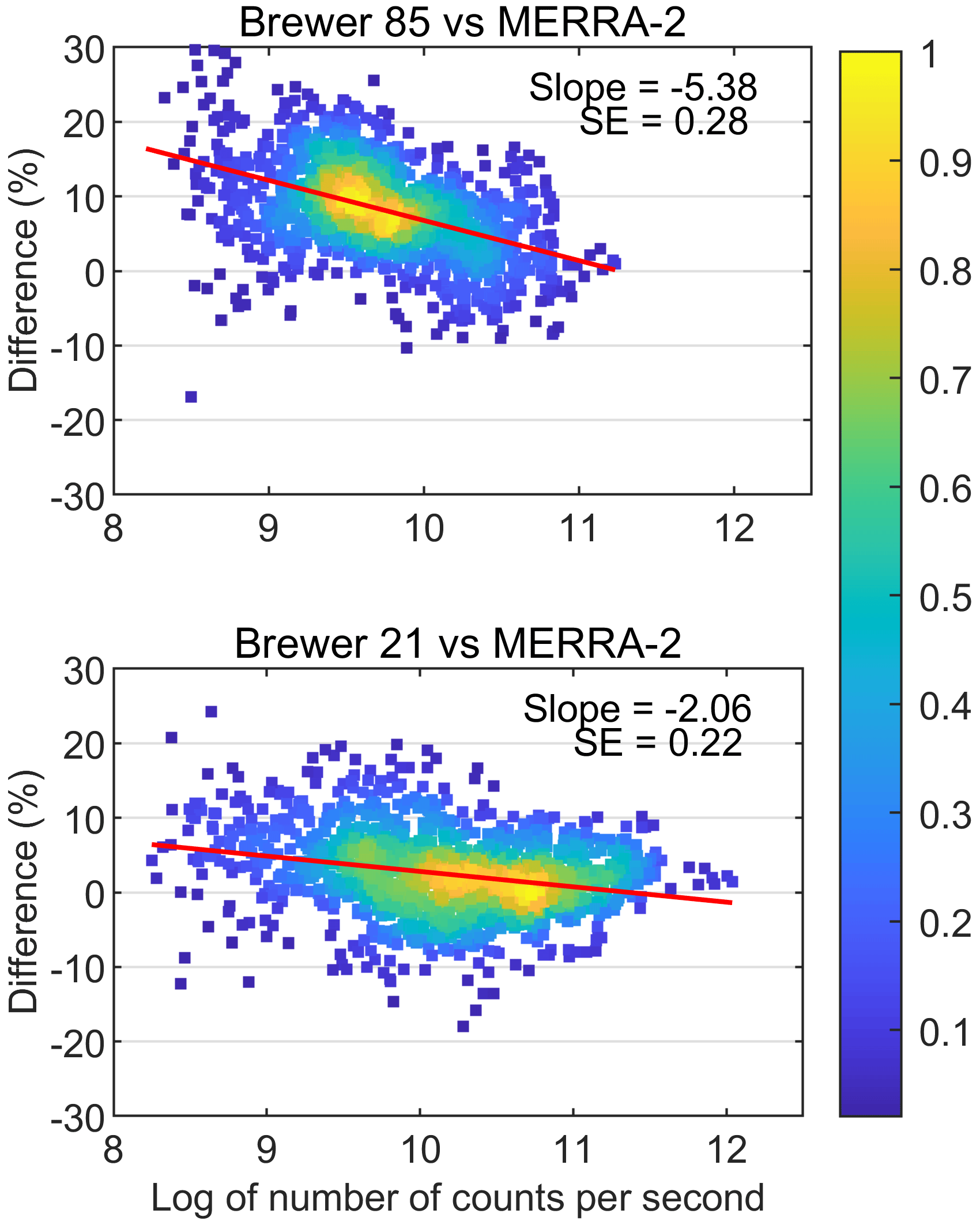
Figure B1Scatter plots of the difference between Brewer FM total ozone and MERRA-2 reanalysis as a function of the natural logarithm of the adjusted number of photon counts per second at Brewer slit 5 (approximately 320 nm). The number of counts was adjusted for the dead time, the number of “dark” counts, and instrument temperature response. The slope of the linear fit and the standard error (SE) of the slope are also shown. The color scale shows the normalized density of the points.
It is important to note that the applied empirical correction did not change the wintertime mean total ozone values for the two Brewer instruments compared to the scenario in which all data with Signal 320 less than 10.5 were discarded. For the latter scenario, the mean wintertime ozone values measured by Brewers 85 (in 2008–2014) and 21 (in 2015–2022) were 244 and 241 DU, respectively, while for the corrected data, they were 244 and 242 DU, respectively. Thus, the correction did not change the average ozone level established by the most reliable Brewer FM measurements. The correction also improved the correlation coefficients between Brewer data and the other datasets. The correlation coefficients of Brewer daily values with Dobson, MERRA-2, and ozonesonde were 0.59, 0.71, and 0.65, respectively, for the original data and 0.73, 0.8, and 0.74 for the adjusted data.
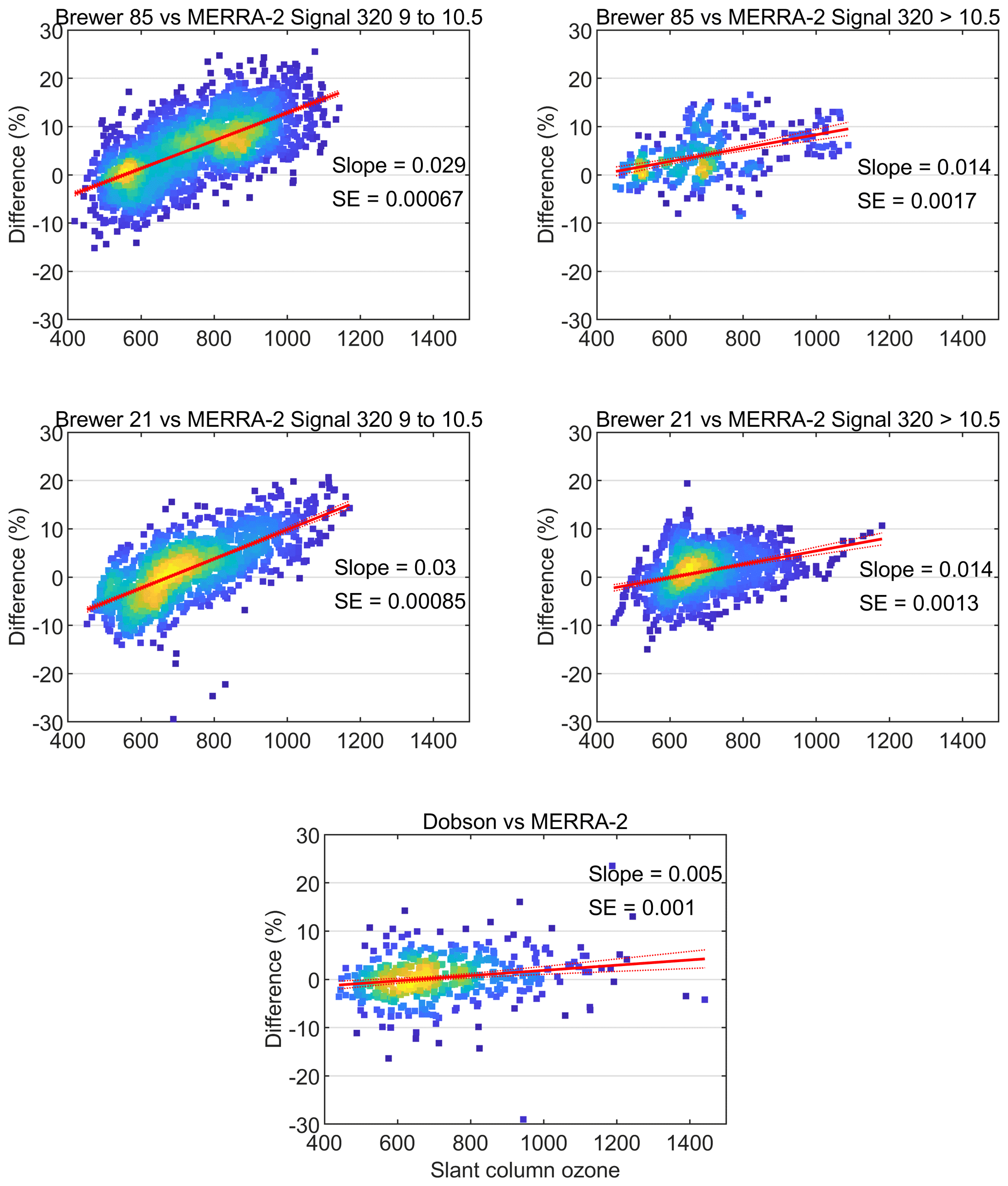
Figure B2Scatter plots of the difference between Brewer and MERRA-2 total ozone as a function of slant column in Dobson units (DU). The best-fit linear regression line, its slope value, and the standard error (SE) of the slope are also shown. The difference is plotted for Brewers 21 and 85 as indicated and for two ranges on Signal 320 values: from 9 to 10.5 and greater that 10.5. The color scale shows the normalized density of the points. A similar plot for all Dobson data is show for comparison.
Brewer data at the South Pole Station are available from the World Meteorological Organization Global Atmosphere Watch Program World Ozone and Ultraviolet Radiation Data Centre (WOUDC): (https://doi.org/10.14287/10000001, ECCC, 2023). Ozonesonde data at the South Pole Station are available from NOAA's Global Monitoring Laboratory (https://gml.noaa.gov/aftp/data/ozwv/Ozonesonde/ NOAA, 2023a). The Dobson and adjusted Brewer FM data are available from https://gml.noaa.gov/aftp/data/ozwv/Dobson/Publications/ (NOAA, 2023b). MERRA-2 data are available from NASA's Global Modelling and Assimilation Office (https://gmao.gsfc.nasa.gov/reanalysis/MERRA-2/, EarthData, 2022).
VF analyzed the data with help from XZ and IA and prepared the paper, with critical feedback from all co-authors. CTM installed the Brewer instrument at the South Pole Station. MB, RS, AO, VF, TM, and SCL operated and managed the South Pole Brewers. IP, BJJ, PC, JB, KM, and GM operated the South Pole Dobson and performed the ozonesonde measurements.
The contact author has declared that none of the authors has any competing interests.
Publisher's note: Copernicus Publications remains neutral with regard to jurisdictional claims in published maps and institutional affiliations.
This article is part of the special issue “Atmospheric ozone and related species in the early 2020s: latest results and trends (ACP/AMT inter-journal SI)”. It is not associated with a conference.
We would like to acknowledge Christopher Osburn at Lunar Outreach Services for developing a free software package for the Moon phase calculations used in this study. We also acknowledge the logistics support in Antarctica provided by the National Science Foundation, Office of Polar Programs, and Amy Cox for her support in setting up the Brewer instrument. We also would like to thank Mark Weber and an anonymous reviewer for their reviews and suggestions.
This paper was edited by Jayanarayanan Kuttippurath and reviewed by Mark Weber and one anonymous referee.
Allen, D. R., Bevilacqua, R. M., Nedoluha, G. E., Randall, C. E., and Manney, G. L.: Unusual stratospheric transport and mixing during the 2002 Antarctic winter, Geophys. Res. Lett., 30, 1599, https://doi.org/10.1029/2003gl017117, 2003.
Ball, W. T., Alsing, J., Mortlock, D. J., Staehelin, J., Haigh, J. D., Peter, T., Tummon, F., Stübi, R., Stenke, A., Anderson, J., Bourassa, A., Davis, S. M., Degenstein, D., Frith, S., Froidevaux, L., Roth, C., Sofieva, V., Wang, R., Wild, J., Yu, P., Ziemke, J. R., and Rozanov, E. V.: Evidence for a continuous decline in lower stratospheric ozone offsetting ozone layer recovery, Atmos. Chem. Phys., 18, 1379–1394, https://doi.org/10.5194/acp-18-1379-2018, 2018.
Basher, R. E.: Review of the Dobson spectrophotometer and its accuracy, WMO Global Ozone Res. Monit. Proj. Rep. 13, World Meteorol. Organ., Geneva, Switzerland, https://library.wmo.int/records/item/50151-review-of-the-dobson-spectrophotometer-and-its-accuracy (last access: 4 October 2023), 1982.
Bass, A. M. and Paur, R. J.: The ultraviolet cross-sections of ozone: I. The measurements, in Atmospheric Ozone, Springer, Germany, 606–610, https://doi.org/10.1007/978-94-009-5313-0_120, 1985.
Bernhard, G., Evans, R. D., Labow, G. J., and Oltmans, S. J.: Bias in Dobson total ozone measurements at high latitudes due to approximations in calculations of ozone absorption coefficients and air mass, J. Geophys. Res., 110, D10305, https://doi.org/10.1029/2004JD005559, 2005.
Bhartia, P. K. and McPeters, R D.: The discovery of the Antarctic Ozone Hole, Comptes Rendus Geoscience, 350, 335–340, https://doi.org/10.1016/j.crte.2018.04.006, 2018.
Brewer, A. W.: A replacement for the Dobson spectrophotometer?, Pure Appl. Geophys., 106, 919–927, 1973.
Brönnimann, S., Staehelin, J., Farmer, S. F. G., Cain, J. C., Svendby, T. M., and Svenøe, T.: Total ozone observations prior to the IGY. I: A history, Q. J. Roy. Meteorol. Soc., 129, 2797–2817, https://doi.org/10.1256/qj.02.118, 2003.
Chubachi, S.: Preliminary result of ozone observations at Syowa Station from February 1982 to January 1983, Memoirs of the National Institute of Polar Research Japanese Special Issue, 34, 13–20, 1984.
de Laat, A. T. J., van der A, R. J., and van Weele, M.: Tracing the second stage of ozone recovery in the Antarctic ozone-hole with a “big data” approach to multivariate regressions, Atmos. Chem. Phys., 15, 79–97, https://doi.org/10.5194/acp-15-79-2015, 2015.
Dobson, G. M. B.: Forty Years' Research on Atmospheric Ozone at Oxford: a History, Appl. Optics., 7, 387–405, https://doi.org/10.1364/ao.7.000387, 1968.
Dobson, G. M. B. and Harrison D. N.: Measurements of the amount of ozone in the Earth's atmosphere and its relation to other geophysical conditions, P. Roy. Soc. Lond. A, 110, 660–693, 1926.
EarthData: MERRA-2 tavg1_2d_slv_Nx: 2d, 1-Hourly, Time-Averaged, Single-Level, Assimilation, Single-Level Diagnostics V5.12.4 (M2T1NXSLV), NASA [data set], https://gmao.gsfc.nasa.gov/reanalysis/MERRA-2/, last access: 1 November 2022.
ECCC: World Meteorological Organization-Global Atmosphere Watch Program (WMO-GAW)/World Ozone and Ultraviolet Radiation Data Centre (WOUDC), https://doi.org/10.14287/10000001, 2023.
Evans, R. D., Petropavlovskikh, I., McClure-Begley, A., McConville, G., Quincy, D., and Miyagawa, K.: Technical note: The US Dobson station network data record prior to 2015, re-evaluation of NDACC and WOUDC archived records with WinDobson processing software, Atmos. Chem. Phys., 17, 12051–12070, https://doi.org/10.5194/acp-17-12051-2017, 2017.
Farman, J. C., Gardiner, B. G., and Shanklin, J. D.: Large losses of total ozone in Antarctica reveal seasonal Clox/NOx interaction, Nature, 315, 207–210, https://doi.org/10.1038/315207a0, 1985.
Fioletov, V., Tarasick, D., and Petropavlovskikh, I.: Estimating ozone variability and instrument uncertainties from SBUV(/2), ozonesonde, Umkehr, and SAGE II measurements: Short-term variations, J. Geophys. Res., 111, D02305, https://doi.org/10.1029/2005jd006340, 2006.
Fioletov, V. E. and Shepherd T. G.: Summertime total ozone variations over middle and polar latitudes, Geophys. Res. Lett., 32, L04807, https://doi.org/10.1029/2004GL022080, 2005.
Fioletov, V. E., Bodeker, G. E., Miller, A. J., McPeters, R. D., and Stolarski, R.: Global and zonal total ozone variations estimated from ground-based and satellite measurements: 1964–2000, J. Geophys. Res., 107, 4647, https://doi.org/10.1029/2001JD001350, 2002.
Fioletov, V. E., Kerr, J. B., McElroy, C. T., Wardle, D. I., Savastiouk, V., and Grajnar, T. S.: The Brewer reference triad, Geophys. Res. Lett., 32, L20805, https://doi.org/10.1029/2005GL024244, 2005.
Fioletov, V. E., Labow, G. , Evans, R., Hare, E. W., Köhler, U., McElroy, C. T., Miyagawa, K., Redondas, A.., Savastiouk, V., Shalamyansky, A. M., Staehelin, J., Vanicek, K., and Weber, M.: Performance of the ground-based total ozone network assessed using satellite data, J. Geophys. Res., 113, D14313, https://doi.org/10.1029/2008JD009809, 2008.
Frith, S. M., Kramarova, N. A., Stolarski, R. S., McPeters, R. D., Bhartia, P. K., and Labow, G. J.: Recent changes in total column ozone based on the SBUV Version 8.6 Merged Ozone Data Set, J. Geophys. Res.-Atmos., 119, 9735–9751, https://doi.org/10.1002/2014JD021889, 2014.
Gelaro, R., McCarty, W., Suárez, M. J., Todling, R., Molod, A., Takacs, L., Randles, C. A., Darmenov, A., Bosilovich, M. G., Reichle, R., Wargan, K., Coy, L., Cullather, R., Draper, C., Akella, S., Buchard, V., Conaty, A., da Silva, A. M., Gu, W., Kim, G.-K., Koster, R., Lucchesi, R., Merkova, D., Nielsen, J. E., Partyka, G., Pawson, S., Putman, W., Rienecker, M., Schubert, S. D., Sienkiewicz, M., and Zhao, B.: The Modern-Era Retrospective Analysis for Research and Applications, Version 2 (MERRA-2), J. Climate, 30, 5419–5454, https://doi.org/10.1175/JCLI-D-16-0758.1, 2017.
Gröbner, J., Schill, H., Egli, L., and Stübi, R.: Consistency of total column ozone measurements between the Brewer and Dobson spectroradiometers of the LKO Arosa and PMOD/WRC Davos, Atmos. Meas. Tech., 14, 3319–3331, https://doi.org/10.5194/amt-14-3319-2021, 2021.
Grubbs, F. E.: On estimating precision of measuring instruments and product variability, J. Am. Stat. Assoc., 43, 243–264, 1948.
Hassler, B., Daniel, J. S., Johnson, B. J., Solomon, S., and Oltmans S. J.: An assessment of changing ozone loss rates at South Pole: Twenty-five years of ozonesonde measurements, J. Geophys. Res., 116, D22301, https://doi.org/10.1029/2011JD016353, 2011.
Hofmann, D. J., Oltmans, S. J., Harris, J. M., Johnson, B. J., and Lathrop, J. A.: Ten years of ozonesonde measurements at the south pole: Implications for recovery of springtime Antarctic ozone, J. Geophys. Res.-Atmos., 102, 8931–8943, https://doi.org/10.1029/96jd03749, 1997.
Hofmann, D. J., Johnson, B. J., and Oltmans, S. J.: Twenty-two years of ozonesonde measurements at the South Pole, Int. J. Remote. Sens., 30, 3995–4008, https://doi.org/10.1080/01431160902821932, 2009.
Hoppel, K., Bevilacqua, R., Allen, D., Nedoluha, G., and Randall, C.: POAM III observations of the anomalous 2002 Antarctic ozone hole, Geophys. Res. Lett., 30, 1394, https://doi.org/10.1029/2003gl016899, 2003.
Johnson, B. J., Cullis, P., Booth, J., Petropavlovskikh, I., McConville, G., Hassler, B., Morris, G. A., Sterling, C., and Oltmans, S.: South Pole Station ozonesondes: variability and trends in the springtime Antarctic ozone hole 1986–2021, Atmos. Chem. Phys., 23, 3133–3146, https://doi.org/10.5194/acp-23-3133-2023, 2023.
Karpetchko, A., Kyro, E., and Knudsen, B. M.: Arctic and Antarctic polar vortices 1957–2002 as seen from the ERA-40 reanalyses, J. Geophys. Res., 110, D21109, https://doi.org/10.1029/2005JD006113, 2005.
Kerr, J. B.: New methodology for deriving total ozone and other atmospheric variables from Brewer spectrophotometer direct sun spectra, J. Geophys. Res.-Atmos., 107, 4731, https://doi.org/10.1029/2001JD001227, 2002.
Kerr, J. B.: The Brewer Spectrophotometer, in: UV Radiation in Global Climate Change: Measurements, Modeling and Effects on Ecosystems, edited by: Gao, W., Slusser, J. R., and Schmoldt, D. L., Springer, Berlin, Heidelberg, 160–191, https://doi.org/10.1007/978-3-642-03313-1_6, 2010.
Kerr, J. B., McElroy, C. T., and Olafson, R. A.: Measurements of ozone with the Brewer ozone spectrophotometer, in: Proceedings of the Quadrennial Ozone Symposium, Boulder, USA, 4–9 August, 1980, 74–79, https://books.google.ca/books/about/Proceedings_of_the_Quadrennial_Internati.html?id=ubZsvwEACAAJ&redir_esc=y (last access: 4 October 2023), 1981.
Komhyr, W. D.: Nonreactive gas sampling pump, Rev. Sci. Instrum., 38, 981–983, https://doi.org/10.1063/1.1720949, 1967.
Komhyr, W. D.: Dobson spectrophotometer systematic total ozone measurement error, Geophys. Res. Lett., 7, 161–163., 1980.
Komhyr, W. D. and Evans R. D.: Operations Handbok – Ozone Observations with a Dobson Spectrophotometer Revised 2008, WMO Global Ozone Res. Monit. Proj. Rep. 183, World Meteorol. Organ., Geneva, Switzerland, 85 pp., https://gml.noaa.gov/ozwv/dobson/GAW183-Dobson-WEB.pdf (last access: 4 October 2023), 2008.
Komhyr, W. D., Grass, R. D., and Leonard, R. K.: Total ozone decrease at South Pole, Antarctica, 1964–1985, Geophys. Res. Lett., 13, 1248–1252, https://doi.org/10.1029/GL013i012p01248, 1986.
Komhyr, W. D., Oltmans, S. J., and Grass, R. D.: Atmospheric ozone at South Pole, Antarctica, in 1986, J. Geophys. Res., 93, 5167–5184, https://doi.org/10.1029/JD093iD05p05167, 1988.
Komhyr, W. D., Grass, R. D., and Leonard R. K.: Dobson spectrophotometer 83: A standard for total ozone measurements, 1962–1987, J. Geophys. Res., 94, 9847–9861, 1989a.
Komhyr, W. D., Grass, R. D., Reitelbach, P. J., Kuester, S. E., Franchois, P. R., and Fanning, M. L.: Total ozone, ozone vertical distributions, and stratospheric temperatures at South Pole, Antarctica, in 1986 and 1987, J. Geophys. Res., 94, 11429–11436, https://doi.org/10.1029/JD094iD09p11429, 1989b.
Komhyr, W. D., Mateer, C. L. and Hudson, R. D.: Effective Bass-Paur 1985 ozone absorption coefficients for use with Dobson ozone spectrophotometers, J. Geophys. Res., 98, 20451–20465, 1993.
Kuttippurath, J., Bodeker, G. E., Roscoe, H. K., and Nair, P. J.: A cautionary note on the use of EESC-based regression analysis for ozone trend studies, Geophys. Res. Lett., 42, 162–168, https://doi.org/10.1002/2014GL062142, 2015.
McElroy, C. T., Savastiouk V., Evans, R. D., Oltmans, S., Booth, J., and Cox, A.: Two Years of Ozone Observations from the South Pole Brewer, in: Geophysical Research Abstracts Vol. 12, EGU2010-15010, EGU General Assembly 2010, https://meetingorganizer.copernicus.org/EGU2010/EGU2010-15010.pdf (last access: 4 October 2023), 2010.
McPeters, R. D. and Labow, G. J.: Climatology 2011: An MLS and sonde derived ozone climatology for satellite retrieval algorithms, J. Geophys. Res., 117, D10303, https://doi.org/10.1029/2011JD017006, 2012.
McPeters, R. D., Labow, G. J., and Johnson, B. J.: A satellite-derived ozone climatology for balloonozonesonde estimation of total column ozone, J. Geophys. Res.-Atmos., 102, 8875–8885, https://doi.org/10.1029/96jd02977, 1997.
McPeters, R. D., Bhartia, P. K., Haffner, D., Labow, G., and Flynn, L.: The version 8.6 SBUV ozone data record: an overview, J. Geophys. Res., 118, 1–8, https://doi.org/10.1002/jgrd.50597, 2013.
Milinevsky, G., Evtushevsky, O., Klekociuk, A., Wang, Y., Grytsai, A., Shulga, V., and Ivaniha, O.: Early indications of anomalous behaviour in the 2019 spring ozone hole over Antarctica, Int. J. Remote Sens., 41, 7530–7540, https://doi.org/10.1080/2150704x.2020.1763497, 2020.
Nash, E. R., Newman, P. A., Rosenfield, J. E., and Schoeberl, M. R.: An objective determination of the polar vortex using Ertel's potential vorticity, J. Geophys. Res.-Atmos., 101, 9471–9478, https://doi.org/10.1029/96jd00066, 1996.
Newman, P. A., Daniel, J. S., Waugh, D. W., and Nash, E. R.: A new formulation of equivalent effective stratospheric chlorine (EESC), Atmos. Chem. Phys., 7, 4537–4552, https://doi.org/10.5194/acp-7-4537-2007, 2007.
NOAA Earth System Research Laboratories, Global Monitoring Laboratory: Ozonesonde data, NOAA [data set], https://gml.noaa.gov/aftp/data/ozwv/Ozonesonde/ (last access: 4 October 2023), 2023a.
NOAA Earth System Research Laboratories, Global Monitoring Laboratory: Dobson Data, NOAA [data set], https://gml.noaa.gov/aftp/data/ozwv/Dobson/Publications/, last access: 4 October 2023, 2023b.
Redondas, A., Evans, R., Stuebi, R., Köhler, U., and Weber, M.: Evaluation of the use of five laboratory-determined ozone absorption cross sections in Brewer and Dobson retrieval algorithms, Atmos. Chem. Phys., 14, 1635–1648, https://doi.org/10.5194/acp-14-1635-2014, 2014.
Ricaud, P., Lefèvre, F., Berthet, G., Murtagh, D., Llewellyn, E. J., Mégie, G., Kyrölä, E., Leppelmeier, G. W., Auvinen, H., Boonne, C., Brohede, S., Degenstein, D. A., de La Noë, J., Dupuy, E., El Amraoui, L., Eriksson, P., Evans, W. F. J., Frisk, U., Gattinger, R. L., Girod, F., Haley, C. S., Hassinen, S., Hauchecorne, A., Jimenez, C., Kyrö, E., Lautié, N., Le Flochmoën, E., Lloyd, N. D., McConnell, J. C., McDade, I. C., Nordh, L., Olberg, M., Pazmino, A., Petelina, S. V., Sandqvist, A., Seppälä, A., Sioris, C. E., Solheim, B. H., Stegman, J., Strong, K., Taalas, P., Urban, J., von Savigny, C., von Scheele, F., and Witt, G.: Polar vortex evolution during the 2002 Antarctic major warming as observed by the Odin satellite, J. Geophys. Res.-Atmos., 110, D05302, https://doi.org/10.1029/2004JD005018, 2005.
Rienecker, M. M., Suarez, M. J., Gelaro, R., Todling, R., Bacmeister, J., Liu, E., Bosilovich, M. G., Schubert, S. D., Takacs, L., and Kim, G.-K.: MERRA: NASA's modern-era retrospective analysis for research and applications, J. Climate, 24, 3624–3648, 2011.
Safieddine, S., Bouillon, M., Paracho, A. C., Jumelet, J., Tence, F., Pazmino, A., Goutail, F., Wespes, C., Bekki, S., Boynard, A., Hadji-Lazaro, J., Coheur, P. F., Hurtmans, D., and Clerbaux, C.: Antarctic ozone enhancement during the 2019 sudden stratospheric warming event, Geophys. Res. Lett., 47, e2020GL087810, https://doi.org/10.1029/2020GL087810, 2020.
Siani, A. M., Frasca, F., Scarlatti, F., Religi, A., Diémoz, H., Casale, G. R., Pedone, M., and Savastiouk, V.: Examination on total ozone column retrievals by Brewer spectrophotometry using different processing software, Atmos. Meas. Tech., 11, 5105–5123, https://doi.org/10.5194/amt-11-5105-2018, 2018.
Solomon, S., Garcia, R. R., Rowland, F. S. and Wuebbles, D. J.: On the depletion of Antarctic ozone, Nature, 321, 755–758, https://doi.org/10.1038/321755a0, 1986.
Solomon, S., Portmann, R. W., Sasaki, T., Hofmann, D. J., and Thompson, D. W. J.: Four decades of ozonesonde measurements over Antarctica, J. Geophys. Res.-Atmos., 110, D21311, https://doi.org/10.1029/2005jd005917, 2005.
Steinbrecht, W. I. Hegglin, M. I., Harris, N., and Weber, M.: Is global ozone recovering?, Comptes Rendus Geoscience, 350, 7, 368–375, https://doi.org/10.1016/j.crte.2018.07.012, 2018.
Sterling, C. W., Johnson, B. J., Oltmans, S. J., Smit, H. G. J., Jordan, A. F., Cullis, P. D., Hall, E. G., Thompson, A. M., and Witte, J. C.: Homogenizing and estimating the uncertainty in NOAA's long-term vertical ozone profile records measured with the electrochemical concentration cell ozonesonde, Atmos. Meas. Tech., 11, 3661–3687, https://doi.org/10.5194/amt-11-3661-2018, 2018.
Stolarski, R. S., Krueger, A. J., Schoeberl, M. R., McPeters, R. D., Newman, P. A., and Alpert, J. C.: Nimbus 7 satellite measurements of the springtime Antarctic ozone decrease, Nature, 322, 808–811, https://doi.org/10.1038/322808a0, 1986.
Stolarski, R. S., Douglass, A. R., Steenrod, S., and Pawson, S.: Trends in stratospheric ozone: Lessons learned from a 3D chemical transport model, J. Atmos. Sci., 63, 1028–1041, 2006.
Toohey, M. and Strong, K.: Estimating biases and error variances through the comparison of coincident satellite measurements, J. Geophys. Res., 112, D13306, https://doi.org/10.1029/2006JD008192, 2007.
Vyushin, D., Fioletov, V. E., and Shepherd, T. G.: Impact of long-range correlations on trend detection in total ozone, J. Geophys. Res., 112, D14307, https://doi.org/10.1029/2006JD008168, 2007.
Wardle, D. I., McElroy, C. T., Kerr, J. B., Wu, E. and Lamb, K.: Laboratory tests on the double Brewer spectrophotometer, in Proceedings of the Quadrennial Ozone Symposium, L'Aquila, Italy, 12–21 September 1996, 997–1000, 1996.
Wargan, K., Labow, G., Frith, S., Pawson, S., Livesey, N., and Partyka, G.: Evaluation of the Ozone Fields in NASA's MERRA-2 Reanalysis, J. Climate, 30, 2961–2988, https://doi.org/10.1175/JCLI-D-16-0699.1, 2017.
Wargan, K., Weir, B., Manney, G. L., Cohn, S. E., and Livesey, N. J.: The Anomalous 2019 Antarctic Ozone Hole in the GEOS Constituent Data Assimilation System With MLS Observations, J. Geophys. Res.-Atmos., 125, e2020JD033335, https://doi.org/10.1029/2020jd033335, 2020.
Waugh, D. and Polvani, L.: Stratospheric Polar Vortices, American Geophysical Union Geophysical Monograph Series, American Geophysical Union, Washington, DC, 43–57, https://agupubs.onlinelibrary.wiley.com/doi/book/10.1029/GM190 (last access: 4 October 2023), 2010.
Waugh, D. W. and Randel, W. J.: Climatology of Arctic and Antarctic polar vortices using elliptical diagnostics, J. Atmos. Sci., 56, 1594–1613, 1999.
Weber, M., Coldewey-Egbers, M., Fioletov, V. E., Frith, S. M., Wild, J. D., Burrows, J. P., Long, C. S., and Loyola, D.: Total ozone trends from 1979 to 2016 derived from five merged observational datasets – the emergence into ozone recovery, Atmos. Chem. Phys., 18, 2097–2117, https://doi.org/10.5194/acp-18-2097-2018, 2018.
Weber, M., Arosio, C., Coldewey-Egbers, M., Fioletov, V. E., Frith, S. M., Wild, J. D., Tourpali, K., Burrows, J. P., and Loyola, D.: Global total ozone recovery trends attributed to ozone-depleting substance (ODS) changes derived from five merged ozone datasets, Atmos. Chem. Phys., 22, 6843–6859, https://doi.org/10.5194/acp-22-6843-2022, 2022.
WMO – World Meteorological Organization: Scientific Assessment of Ozone Depletion: 2018, Global Ozone Research and Monitoring Project – Report No. 58, Geneva, Switzerland, 572 pp., https://csl.noaa.gov/assessments/ozone/2018/ (last access: 4 October 2023), 2018.
WMO – World Meteorological Organization: Scientific Assessment of Ozone Depletion: 2022, GAW Report No. 278, WMO, Geneva, Switzerland, 509 pp., https://csl.noaa.gov/assessments/ozone/2022/ (last access: 4 October 2023), 2022.
Wohltmann, I., Lehmann, R., Rex, M., Brunner, D., and Mäder J. A.:, A process-oriented regression model for column ozone, J. Geophys. Res., 112, D12304, https://doi.org/10.1029/2006JD007573, 2007.
Zhao, X., Fioletov, V., Cede, A., Davies, J., and Strong, K.: Accuracy, precision, and temperature dependence of Pandora total ozone measurements estimated from a comparison with the Brewer triad in Toronto, Atmos. Meas. Tech., 9, 5747–5761, https://doi.org/10.5194/amt-9-5747-2016, 2016.
Zhao, X., Weaver, D., Bognar, K., Manney, G., Millán, L., Yang, X., Eloranta, E., Schneider, M., and Strong, K.: Cyclone-induced surface ozone and HDO depletion in the Arctic, Atmos. Chem. Phys., 17, 14955–14974, https://doi.org/10.5194/acp-17-14955-2017, 2017.
Zhao, X., Bognar, K., Fioletov, V., Pazmino, A., Goutail, F., Millán, L., Manney, G., Adams, C., and Strong, K.: Assessing the impact of clouds on ground-based UV-visible total column ozone measurements in the high Arctic, Atmos. Meas. Tech., 12, 2463–2483, https://doi.org/10.5194/amt-12-2463-2019, 2019.
Zhao, X., Fioletov, V., Brohart, M., Savastiouk, V., Abboud, I., Ogyu, A., Davies, J., Sit, R., Lee, S. C., Cede, A., Tiefengraber, M., Müller, M., Griffin, D., and McLinden, C.: The world Brewer reference triad – updated performance assessment and new double triad, Atmos. Meas. Tech., 14, 2261–2283, https://doi.org/10.5194/amt-14-2261-2021, 2021.
- Abstract
- Introduction
- Instruments and datasets
- Comparison of the data records
- Long-term changes in wintertime total ozone
- Discussion and conclusion
- Appendix A: The lunar disk illumination and lunar zenith angles
- Appendix B: Brewer data corrections
- Data availability
- Author contributions
- Competing interests
- Disclaimer
- Special issue statement
- Acknowledgements
- Review statement
- References