2.1 Campaign overview

The expedition PS106 of the research vessel Polarstern (Knust, 2017) was conducted between the end of May and mid-July 2017 in the Arctic Ocean (Wendisch et al., 2019). The measurements were performed as part of the PASCAL (Physical Feedbacks of Arctic Boundary Layer, Sea Ice, Cloud and Aerosol) campaign in the framework of the German Arctic Amplification: Climate Relevant Atmospheric and Surface Processes, and Feedback Mechanisms (AC)³ project.

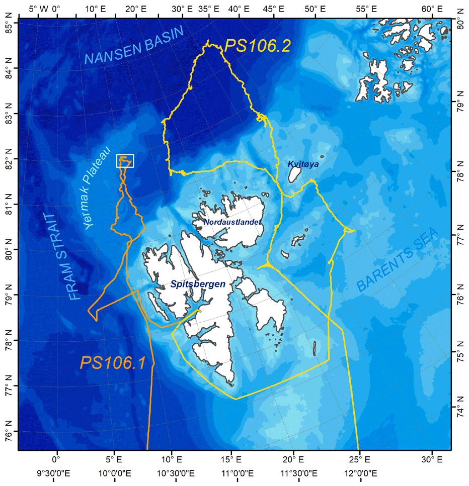
Figure 1Overview of the main expedition area of the Polarstern cruises PS106.1 and PS106.2. Figure taken from Macke and Flores (2018).

The first leg (PS106.1) started on 24 May in Bremerhaven (Germany) and ended on 21 June in Longyearbyen (Svalbard) and featured a 10 d ice floe camp that was set up between 5 and 14 June 2017. The main area of investigation was the Arctic Ocean a few hundred kilometers northwest of Svalbard (see Fig. 1).

The expedition continued with its second leg (PS106.2) on 23 June from Lonyearbyen and ended on 20 July in Tromsø (Norway). In comparison to PS106.1, the second leg focused on the area northeast of Svalbard, went up to higher latitudes (up to 83.7^∘ N), and the vessel did not stop for extended stays at an ice floe.

As an overview about the meteorological situation during the campaign, Fig. S1 in the Supplement shows the frequency distributions for all meteorological parameters that were continuously measured on Polarstern. The mean and standard deviation of air temperature (T_air), relative humidity (RH), and atmospheric pressure (p) are given in the following: for the whole first leg they are $T_{\mathrm{air}}=-\mathrm{0.01}$ ^∘C ± 4.21 ^∘C, RH=90.70 % ± 10.62 %, and p=1016.36 hPa ± 7.48 hPa, whereas for the second leg the parameters were T_air=0.22 ^∘C ± 2.71 ^∘C, RH=94.82 % ± 6.09 %, and p=1006.84 hPa ± 5.12 hPa. During the time within the ice pack, the averages of these parameters were as follows: $T_{\mathrm{air}}=-\mathrm{1},\mathrm{37}$ ^∘C ± 1.50 ^∘C, RH=94.35 % ± 4.54 %, and p=1011.27 hPa ± 8.52 hPa; out of the ice pack, T_air=4.75 ^∘C ± 3.65 ^∘C, RH=88.03 % ± 11.27 %, and p=1012.92 hPa ± 4.89 hPa.

For further details on the measurement strategy as well as the meteorological, sea ice, and cloud conditions during PASCAL, we refer the reader to Wendisch et al. (2019) and the PS106 cruise report by Macke and Flores (2018).

2.2 Sample collection

In order to gain a comprehensive insight into the abundance and nature of INPs in the Arctic during summertime, samples from different compartments were taken. These included atmospheric, bulk seawater (BSW), sea surface microlayer (SML), and fog samples. All samples were stored on the vessel directly after sampling in a cold room at −20 ^∘C, and it was ensured that the samples stayed below 0 ^∘C during transport to the Leibniz Institute for Tropospheric Research (TROPOS), where they were stored at −24 ^∘C until they were analyzed.

2.3 INP analysis

2.4 Collocated measurements and supporting observations

In addition to the sampling of INPs, the physicochemical properties of the prevailing atmospheric aerosol particles were measured inside a temperature-controlled measurement container located on the monkey island of the RV Polarstern. The temperature inside the container was held at ca. 24 ^∘C, while the aerosol inlet was heated to 30 ^∘C to prevent icing. The aerosol inlet consists of a 6 m long stainless-steel tubing (inner diameter of 40 mm), which faces upwards at a 45^∘ angle to the bow of the ship. The flow through the inlet was set to 40 L min⁻¹ (Reynolds number <2000). With an isokinetic splitter, the aerosol was distributed between the different instruments. The aerosol instrumentation relevant to this study included a mobility particle size spectrometer (MPSS) to measure particle number size distributions (PNSDs), a condensation particle counter (CPC) to measure total particle concentration (N_tot), and a cloud condensation nuclei counter (CCNC) to measure the concentrations of cloud condensation nuclei (N_CCN).

PNSDs in the size range between 10 and 800 nm were measured with a TROPOS-type MPSS (Wiedensohler et al., 2012). The time resolution of an upscan and downscan was 5 min. PNSDs were derived with the inversion algorithm by Pfeifer et al. (2014) and corrected for transmission losses as well as counting efficiencies according to Wiedensohler et al. (1997). The sizing of the MPSS was calibrated according to Wiedensohler et al. (2018) at regular time intervals during the campaign (for further details on the MPSS and the measurement container, we refer the reader to Kecorius et al., 2019). N_tot was measured with a CPC (model 3010, TSI Inc., Shoreview, USA; lower cutoff: 10 nm). A CCNC (CCN-100, DMT, Boulder USA; Roberts and Nenes, 2005) was used to measure N_CCN at six different supersaturation values (SS: 0.1 %, 0.15 %, 0.2 %, 0.3 %, 0.5 %, 1 %,). Each SS level was sampled for 10 min and averaged over that period; hence, a certain SS has a time resolution of 1 h. The instrument was calibrated with ammonium sulfate particles before and after the campaign according to the ACTRIS protocol (Gysel and Stratmann, 2013).

In addition to the offline INP analysis of the filter samples, also the SPectrometer for Ice Nuclei (SPIN; Droplet Measurements Techniques, Boulder, CO, USA) was deployed to measure N_INP in immersion mode online. SPIN is a continuous-flow diffusion chamber (CFDC) with a parallel plate geometry, and the measurement principle of SPIN in immersion mode can be briefly described as follows: aerosol particles are activated to cloud droplets and then exposed to conditions where ice can form. The number of formed ice crystals is then optically detected. SPIN is described in detail in Garimella et al. (2016). SPIN was placed within a measurement container. Together with the other aerosol instrumentation, the aerosol was fed to SPIN through one main inlet but with additional subsequent drying of the aerosol. SPIN sampled in half-hourly intervals of constant temperature and relative humidity, and each sampling condition was repeated three times within 24 h. The SPIN dataset is also part of the overview of global shipborne INP measurements by Welti et al. (2020).

Na⁺ and Cl⁻ mass concentrations on size-resolved ambient aerosol particles were measured from five-stage Berner impactor samples (mounted outside of the measurement container; the setup is described in detail in Kecorius et al., 2019) by ion chromatography (ICS3000, Dionex, Sunnyvale, CA, USA), as described in Müller et al. (2010) in more detail. Ion chromatography was also used to determine the salinity of the seawater samples.

5 d air mass back-trajectories were calculated using the HYbrid Single-Particle Lagrangian Integrated Trajectory (HYSPLIT) model (Rolph et al., 2017; Stein et al., 2015). As input for the model, the GDAS1 meteorological fields (Global Data Assimilation System; 1^∘ latitude/longitude; 3-hourly) were used. Trajectories were initiated at 50, 250, and 1000 m every hour.

The sea ice concentration at the position of Polarstern was determined with the sea ice concentration product of the EUMETSAT Ocean and Sea Ice Satellite Application Facility (OSI-401-b: SSMIS Sea Ice Concentration Maps on 10 km Polar Stereographic Grid; Tonboe et al., 2017).

Chlorophyll a (Chl a) concentration was derived from the vessel's FerryBox system (4H-FerryBox, Jena Engineering, Jena, Germany). A FerryBox is an autonomous online instrument with modular sensor assembly to continuously measure oceanographic parameters in a flow-through system (Petersen et al., 2011, 2007). The data from the Chl a sensor in the FerryBox system were accessed via the DSHIP portal (https://dship.awi.de/, last access: 26 March 2021) provided by the operator of the vessel. Chl a concentrations were also derived from satellite remote sensing (Aqua MODIS, NPP, L3SMI, Global, 4 km, Science Quality, 2003–present, 8 d composite, 8 to 16 July).

3.1 Atmospheric INP concentrations N_INP

A time series of atmospheric N_INP at selected temperatures derived from filter samples and online measurements with SPIN is shown in Fig. 2. The colored areas mark the periods when Polarstern was located in a certain environment (yellow = ice-free ocean; blue = within ice pack; purple = marginal ice zone). Overall N_INP is the highest at the beginning of the campaign, in between both legs at the harbor of Longyearbyen, and upon entering the ice-free ocean again towards the end of the second leg. The lowest concentrations occurred when the vessel was within the ice pack. It can also be seen that, at a given time, peaks appear or disappear depending on temperature, indicating that different populations of INPs contribute at warmer or colder temperatures.

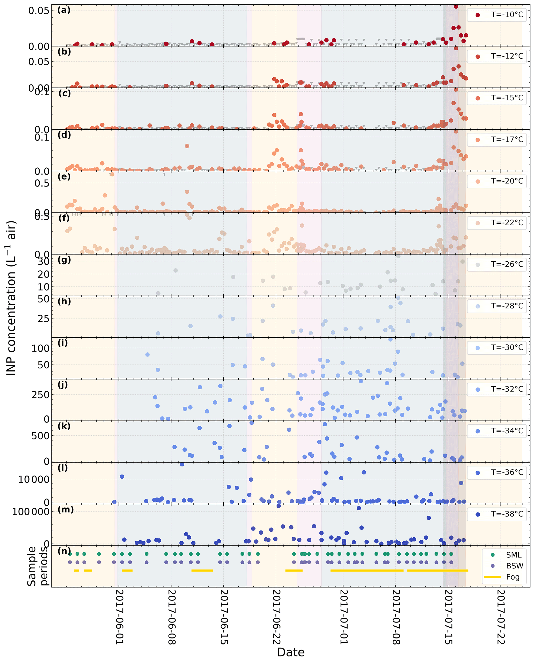
Figure 2Time series of atmospheric N_INP at different temperature derived from filter samples with LINA (−22 ^∘C and above) and SPIN measurements (−26 ^∘C and below). The bottom panel contains markers for the sample collection times of the SML, BSW, and fog water samples. The shaded areas indicate the environment that the vessel is located in (yellow = ice-free ocean; blue = within ice pack; purple = marginal ice zone). The dark gray area indicates the period of the case study discussed in Sect. 3.5. Note that SPIN measurements were only obtained beginning with 31 May.

Download

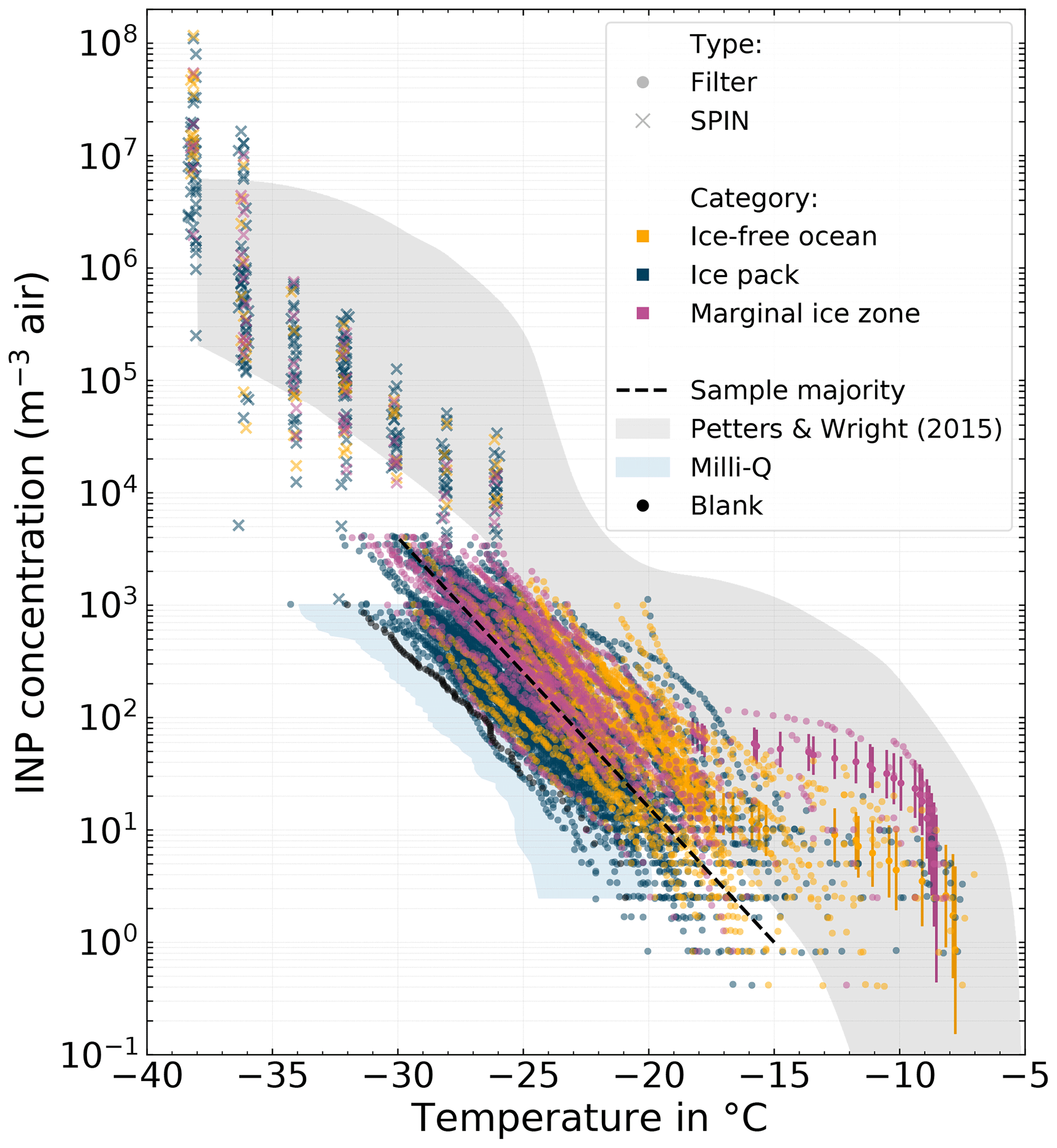
Figure 3All cumulative INP spectra derived from atmospheric filter samples measured with LINA (circle marker), as well as N_INP(T) measured with SPIN (cross marker). The color code refers to the environment the sample was taken from (yellow = ice-free ocean; blue = ice pack; purple = marginal ice zone). The majority of the filter samples are clustered around a line which is shown as a black dashed line. The range of N_INP for midlatitudes by Petters and Wright (2015) is shown as a gray shaded area for reference. The blue areas depicts the 10th to 90th percentile range of all pure Milli-Q measurements with LINA (scaled to atmospheric concentrations with the average sampled air volume of the 8 h samples).

Download

Figure 3 shows the N_INP freezing spectra for the atmospheric filter samples measured with LINA (circle markers), as well as N_INP(T) measured with SPIN (cross markers). The color represents the environment in which the sampling took place, based on the sea ice concentrations at the location of Polarstern (yellow = ice-free ocean; blue = ice pack; purple = marginal ice zone, MIZ). The MIZ is defined as the transitional zone between open sea and dense drift ice. It spans from 15 % to 80 % of the sea surface being covered with ice. The area north of the MIZ is classified as the ice pack, and the area south of the MIZ is classified as ice-free ocean. As the filter samples were collected over the course of several hours on an often moving vessel, the sample environment might change during sampling. In such cases the sample was labeled according to the environment, which accounts for most of the sampling time. The range of N_INP for midlatitudes by Petters and Wright (2015) is shown as a gray shaded area for reference. Additionally, Fig. S10 in the Supplement shows a box plot of the very same filter samples, in order to emphasize the general differences between the environments.

At any particular temperature, N_INP varies between 2 to 3 orders of magnitude. The variability tends to be higher at warmer temperatures compared to colder temperatures: at −10 ^∘C N_INP varies between $\mathrm{4}\times {\mathrm{10}}^{-\mathrm{1}}$ and 6×10¹ m⁻³, at −17 ^∘C between $\mathrm{4}\times {\mathrm{10}}^{-\mathrm{1}}$ and 1×10² m⁻³, and at −25 ^∘C between 3×10¹ and 2×10³ m⁻³. It can be seen that the majority of the samples are clustered around a line ranging roughly from 1 m⁻³ at −15 ^∘C to 4×10³ m⁻³ at −30 ^∘C. But also highly ice-active filter samples featuring N_INP as high as 6×10¹ m⁻³ at −10 ^∘C were observed. These tend to be associated more often with the MIZ (purple symbols) and at −15 ^∘C also with the ice-free ocean (yellow symbols) environment than with the ice pack (see Fig. S10 in the Supplement). We will describe these highly ice-active samples in more detail in Sect. 3.5. In comparison to the range of N_INP from midlatitudes by Petters and Wright (2015), the filter-derived N_INP levels are lower for temperatures below ca. −20 ^∘C, but similar at warmer temperatures. For a given temperature, N_INP measured with SPIN falls within the lower half of the N_INP range by Petters and Wright (2015), with the exception of the two lowest temperature steps.

In Fig. 3 it can be seen that some LINA freezing spectra go up to higher values (4×10³ m⁻³) than others (ending at 1×10³ m⁻³). The cause of this lies in the measurement principle itself: DFAs only measure N_INP per volume of water in a certain concentration range determined by the specific setup configuration. With the known volume of air sampled onto one filter, these concentrations per volume of water are then scaled to atmospheric concentrations per volume of air. Hence differing ranges of resulting values are caused by systematic differences in V_air. In our case we collected samples for 8 or 2 h, and since the flow rate is relatively constant, V_air of the 8 h samples is about 4 times larger than that of the 2 h samples, which causes also the different reported ranges in atmospheric N_INP as seen in Fig. 3. It should also be mentioned that the upper and lower ends of the freezing spectra shown in this work only represent the limits of our detectable range and do not imply that outside these limits no higher N_INP or lower N_INP existed.

The test for heat-labile INPs (Figs. S6 and S7 in the Supplement) demonstrates that ice activity of the samples is reduced when heated for 1 h at 95 ^∘C. Especially INPs that nucleated ice at temperatures above ca. −16 ^∘C are gone after the heating. This is widely seen as an indicator for the presence of biogenic, proteinaceous INPs as those become denatured during the heating, which reduces their ice activity (Conen et al., 2011, 2012, 2017; Conen and Yakutin, 2018; Felgitsch et al., 2018; Hara et al., 2016; Joly et al., 2014; Moffett et al., 2018; Hill et al., 2016; Huang et al., 2021; McCluskey et al., 2018b; Kunert et al., 2019; Pouleur et al., 1992).

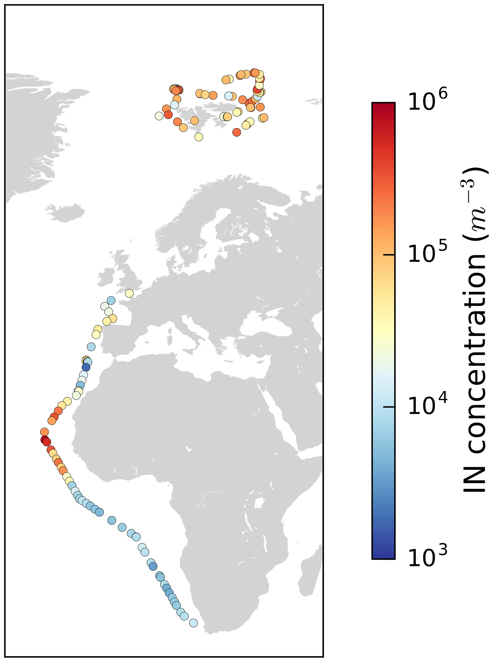
Figure 4Map with color-coded N_INP in the Arctic at −32 ^∘C measured with SPIN during PS106 and also SPIN data of a transect from Bremerhaven (Germany) to Cape Town (South Africa) along the western coast of Africa (Welti et al., 2020).

In the previous section we described that at warmer temperatures, e.g., at −10 ^∘C, samples with high INP concentrations are found more often in the MIZ and less frequently within the ice pack. In comparison, at the lower temperatures measured with SPIN (cross markers in Fig. 4) no correlation with the environmental setting is found. However, in a global context the level of N_INP at these low temperatures is remarkable by itself as shown in Fig. 4. That figure shows N_INP in the Arctic at −32 ^∘C measured with SPIN during PS106 but also SPIN data by Welti et al. (2020) of a transect from Bremerhaven (Germany) to Cape Town (South Africa) along the western coast of Africa. It is striking that at these low temperatures N_INP levels in the Arctic are in the same order of magnitude as in the outflow region of mineral dust from the Sahara. While we have no means of proving the presence of mineral dust at these colder temperatures during PASCAL, to our knowledge there are also no other known sources of INP that can produce such high concentrations throughout the whole time period of the campaign. Also, it was recently shown by Sanchez-Marroquin et al. (2020) that Iceland can be a strong Arctic dust source. Also Irish et al. (2019a) suggested that observed INPs were mineral dust particles originating in the Arctic (Hudson Bay, eastern Greenland, northwest continental Canada) rather than particles originating from sea spray. And global model transport simulations done by Groot Zwaaftink et al. (2016) show that mineral dust is not only transported into the Arctic from remote regions but also, possibly increasingly, generated in the region itself. However, it is also possible also other sources of mineral INPs contribute to the INP population at these temperatures. For example, diatoms represent a biogenic but mineral source of INPs, as they have a cell wall made of silica (Xi et al., 2021). Therefore, it is likely that mineral INPs, possibly mineral dust, contribute to N_INP at low temperatures during the campaign.

3.2 INPs in sea surface microlayer and bulk seawater

Figure 5N_INP in SML and BSW measured with INDA and LINA. Samples are categorized according to the environment (ice-free ocean, ice pack, melt pond, marginal ice zone) the samples were taken from. The gray box indicates the range of values reported by Wilson et al. (2015) for the Arctic. The blue areas depicts the 10th to 90th percentile range of all pure Milli-Q measurements with INDA and LINA.

Download

Figure 5 shows N_INP per volume of water in SML and BSW. Again, the color code refers to the environment the sample was taken from (yellow = ice-free ocean; blue = ice pack; purple = MIZ; green = melt point). The gray box indicates the range of values reported in an earlier study by Wilson et al. (2015) in the Arctic, although they did not separate their samples into different environments. Additionally, Figs. S11 and S12 in the Supplement show box plots of the very same SML and BSW samples in order to emphasize the general differences between the environments.

Both SML and BSW show a high intersample variability. Concentrations for both vary at least between 2 and 3 orders of magnitude at any temperature. Some samples initiate freezing clearly above −10 ^∘C (highest observed freezing onset was at −5.5 ^∘C), while for other samples freezing starts only at temperatures below −15 ^∘C.

It is worth mentioning that the concentration range of INPs reported by Wilson et al. (2015) is not directly comparable to the measurements we present, because due to a different measurement setup, they have different limits of their detectable range. Nevertheless, it can be seen that their SML samples contain up to 2 orders of magnitude higher concentrations of INPs that are ice active at high temperatures (above ca. −10 ^∘C).

Interestingly, some of our samples stand out, i.e., feature significantly higher ice activities at a certain temperature than the majority of the samples (see Fig. 5). The dashed black line in Fig. 5 roughly separates the samples into those that stand out (above the line) and the rest of the very similar samples (below the line). It is noticeable that SML samples from the known biologically active MIZ belong mostly to the group of samples that stand out from the rest. Also the overall most active SML sample originates from the MIZ, and its connection to the corresponding atmospheric filter samples is discussed in more detail in the case study in Sect. 3.5. The high variability of the INP concentrations in SML and BSW in our view is a clear hint towards the sporadic occurrence of INPs in these compartments.

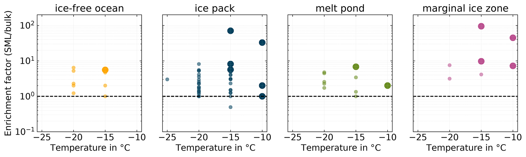
Figure 6Enrichment factors for all pairs of SML and BSW samples (INDA measurements) divided into separate panels by their environmental setting. Larger markers correspond to the pairs of samples for which either the SML or the BSW sample stands out in terms of ice activity.

Download

The SML has been found to be enriched in particulate organic matter and surface-active substances compared to the underlying bulk seawater, with enrichment factors (EFs) of up to 10 and 50, respectively, being reported (Engel et al., 2017; Kuznetsova and Lee, 2002). And, as described in the introduction, the SML is known to be highly ice active. It is therefore an interesting question whether INPs are also enriched in the SML compared to BSW and whether enrichment is a general feature in all samples or if it is restricted to certain situations. To answer this question, we derived INP enrichment factors for the SML, based on corresponding SML and BSW samples as

Figure 6 depicts the calculated EFs at selected temperatures. We observe that the majority of SML samples are enriched in INPs compared to the underlying BSW. The majority of EFs fall into the range between 1 and 10, with only four occurrences of higher values. The highest EF we found was 94.97. There are seven occurrences of EF=1 and only one of EF≤1. This result is similar to Wilson et al. (2015), who only observed enrichment and no depletion of INPs in the SML. On the other hand, the study by Irish et al. (2017) also reports few cases of INPs depletion in the SML. But, as Gong et al. (2020) pointed out, direct comparisons of EFs between different studies are difficult since methodological differences might be of importance.

The larger markers in Fig. 6 indicate samples where the SML showed significantly higher ice activity compared to the others, i.e., higher INP concentrations (see above). Interestingly, almost exclusively the highly ice-active SML samples are the samples which feature the highest EFs, suggesting that enrichment could be an important factor in controlling SML ice activity.

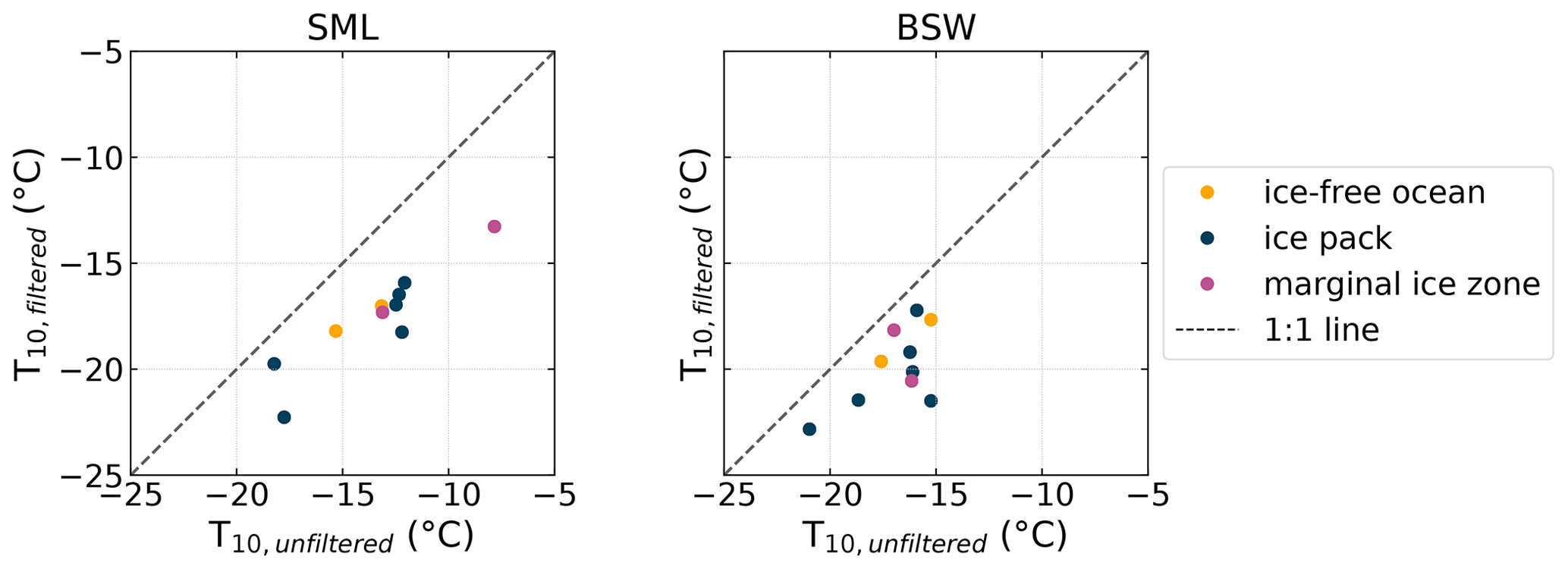
Figure 7Comparison of filtered and unfiltered SML and BSW samples measured with INDA. Shown are the T₁₀ values for corresponding samples. Symbols below the 1:1 line indicate that the filtered sample is less ice active.

Download

Filtrations of 10 randomly selected SML and 12 BSW samples were created and analyzed for N_INP to find indications concerning the size of the INPs present in the samples. The samples were filtered with 0.2 µm PTFE syringe filters (Puradisc 25, Whatman). While the individual sample was chosen randomly, it was ensured that all sample environments (ice-free ocean, ice pack, melt pond, marginal ice zone) were considered. Figure 7 shows a scatter plot of the T₁₀ values, i.e., the temperature where 10 % of the droplets are frozen, of the filtered and unfiltered samples. If a sample falls below the 1:1 line, it indicates that the filtration reduced the ice activity, and the distance to the 1:1 line in the x direction is a measure of how strong the reduction in ice activity is. The complementary plots of the T₅₀ and T₉₀ can be found in the Supplement. Throughout all samples a reduction of the freezing temperatures can be seen due to filtrations. Also, the more ice active the unfiltered sample was, the larger the shift towards lower temperatures tends to be (see also Fig. S4 in the Supplement). The most ice-active sample shifted by around 5 ^∘C, while those with lower initial ice activity only are decreased by approximately 2 ^∘C. This clearly indicates that a high fraction of the INPs are larger or at least associated with particles larger than 0.2 µm.

3.3 INPs in fog water

Analogous to the SML and BSW samples, N_INP was also determined in collected fog water samples. At −10 ^∘C, we find N_INP between the lower limit of our detectable range of 2×10² and 2×10⁴ L⁻¹. At −15 ^∘C, N_INP between 6×10² L⁻¹ and the upper limit of our detectable range 9×10⁴ L⁻¹ were observed. At −20 ^∘C, values between 1×10⁴ L⁻¹ and the upper limit of our detectable range, 9×10⁴ L⁻¹ were found. Fourteen fog samples (63.6 % of all fog samples) have a freezing onset above −10 ^∘C, suggesting the presence of biogenic INPs, as mineral dust only starts to contribute to the INP population at temperatures below −15 ^∘C (e.g., Murray et al., 2012; O'Sullivan et al., 2018). The highest freezing onset we observed in a sample was at −3.47 ^∘C. The samples are divided into two groups by a clearly recognizable gap. The occurrence of these two groups could not directly be related to meteorological parameters. However, as will be discussed in Sect. 3.3.1, the group of more ice-active fog samples may be associated with the more ice-active atmospheric filter samples.

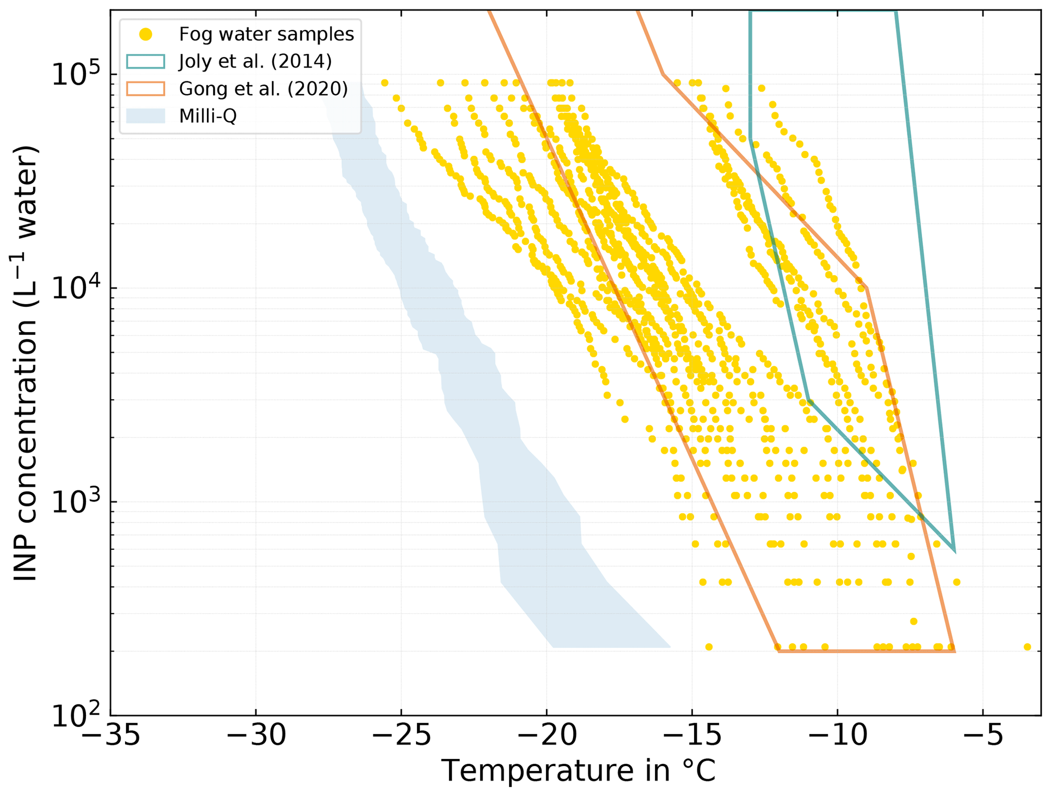
Figure 8N_INP in fog water samples measured with INDA. The teal and orange polygons show the range of values observed by Joly et al. (2014) and Gong et al. (2020), respectively.

Download

In general the fog samples tend to be more ice active and show higher N_INP at a given temperature than the seawater samples presented in Sect. 3.2. A qualitatively similar observation was already made by Schnell (1977). For seawater samples that they collected near Nova Scotia (Canada), they found that some of the samples were very ice active, although the majority of their seawater samples contained no INPs active at temperatures warmer than −14 ^∘C. On the other hand, half of their fog water samples were ice active at temperatures above −10 ^∘C with the most ice-active sample initiating freezing at −2 ^∘C. Schnell (1977) also described that they found N_INP in seawater, fog, and air to vary independently from each other. An observation that also largely applies to this study, but a more detailed investigation of the relation between N_INP in the different compartments is presented in the following Sect. 3.3.1 and 3.4.

The N_INP(T) we observed in Arctic fog water is similar to what Gong et al. (2020) found in cloud water samples on the Cabo Verde islands but tends to be lower than what was observed by Joly et al. (2014), who measured at Puy-de-Dôme (France) and reported a correlation between high concentrations of biological particles and INP concentrations. However the freezing onset temperature of around −6 ^∘C is almost identical in the three studies.

3.3.1 Connecting INPs in clear or fog-free air to fog samples

In this section we relate and compare N_INP in fog water samples with those measured in fog-free air (see Sect. 3.1), following the procedure introduced in Gong et al. (2020), which is briefly described in the following. The number concentration of CCN (N_CCN) at a particular supersaturation (SS) is used as a proxy for the fog droplet number concentration. Furthermore, Gong et al. (2020) made the legitimate assumption, that all INPs act as CCN. Together with an estimated fog droplet diameter (d_drop), the volume of fog water per volume dry air, LWC_fog, can be calculated as follows:

$$\begin{array}{}\text{(5)}& {\mathrm{LWC}}_{\mathrm{fog}}=N_{\mathrm{CCN}}\cdot \mathit{\pi }/\mathrm{6}\cdot d_{\mathrm{drop}}^{\mathrm{3}}.\end{array}$$

For determining N_CCN, a SS needs to be defined. Since fog, unlike clouds, is characterized by low updrafts, SS is also typically low (0.02 %–0.2 %; Pruppacher and Klett, 2010). Thus we choose N_CCN measured at SS=0.15 % as a proxy for the droplet number concentration. Please note that we do not use N_CCN measured at SS=0.1 %, because after the removal of data points due to quality assurance, the data coverage for SS=0.15 % is significantly better than for SS=0.1 %.

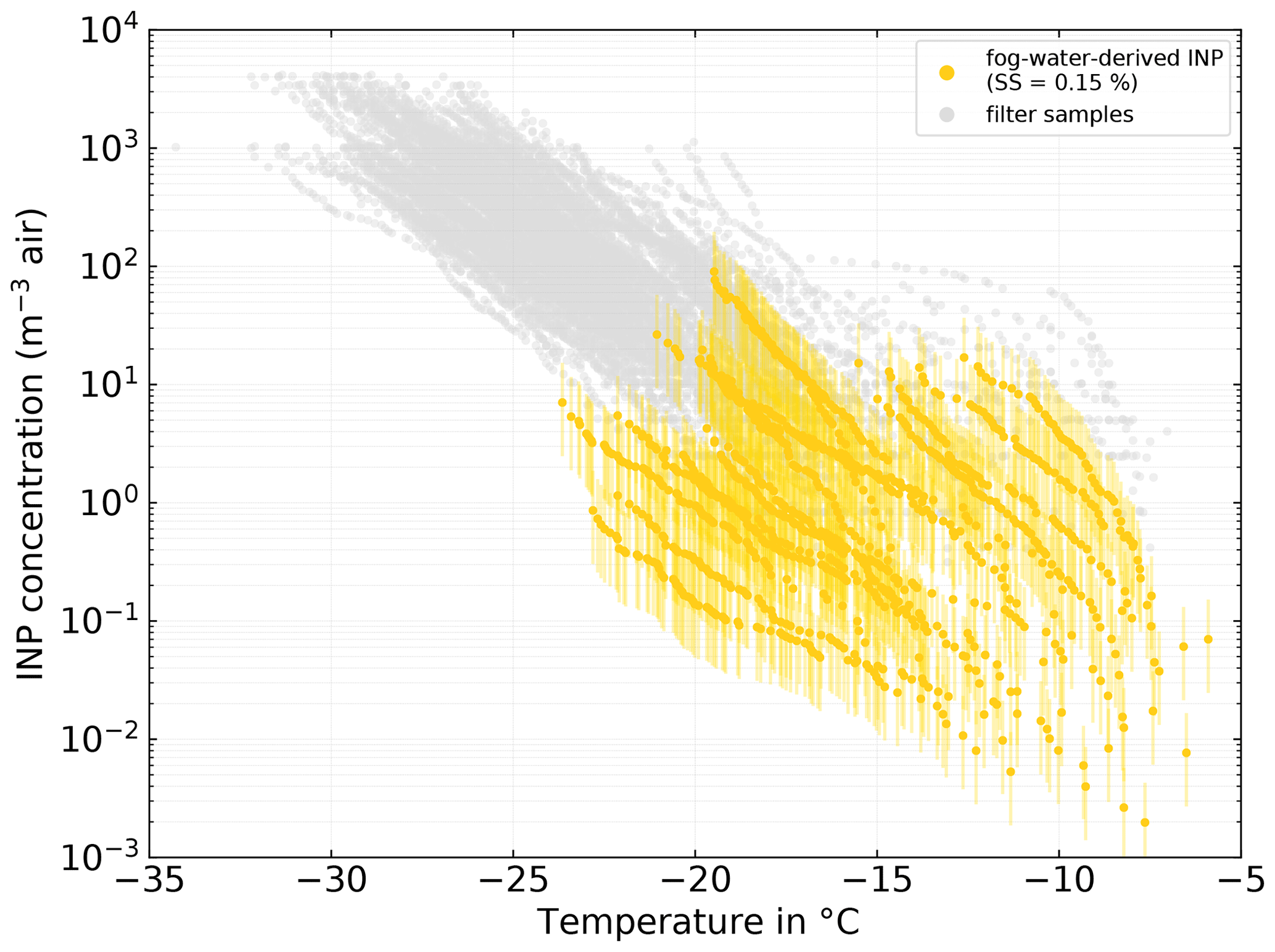
Figure 9Fog-water-derived N_INP in air. N_INP was derived from Eqs. (5) and (6) with the median N_CCN (SS=0.15 %) during the time of each fog sample and an average droplet diameter (d_drop) of 17 µm. The error bars show the range with d_drop of 12 and 22 µm, respectively. See Sect. 3.3.1 for details on the derivation method.

Download

Remote sensing studies of Arctic cloud droplet sizes report typical diameters between 14 and 20 µm (Bierwirth et al., 2013; Shupe et al., 2001; King et al., 2004) and in situ observations found values between 12 and 22 µm. Hence we use 17 µm as an average d_drop and vary it between 12 and 22 µm. With that we calculate a range of LWC_fog, which is then further used to derive the INP number concentration in air, N_INP, air, based on the INP concentration in fog water, N_{INP, fogwater}:

$$\begin{array}{}\text{(6)}& N_{\mathrm{INP},\mathrm{air}}={\mathrm{LWC}}_{\mathrm{fog}}\cdot N_{\mathrm{INP},\mathrm{fogwater}}.\end{array}$$

Figure 9 depicts N_INP as determined from the clear-air filter samples with gray symbols and the ones derived from the fog water samples in yellow. Overall, measured and derived N_INP are in good agreement. Unfortunately, as multiple atmospheric filter samples were taken during the collection time of a single fog sample, an unambiguous attribution of a filter to a fog sample is difficult. Therefore, here we can only report the half-quantitative observation that the freezing spectra of the atmospheric filter samples taken concurrently with the most ice-active fog samples and the spectra derived from the fog water samples feature similar shapes, with the shapes themselves and the onset of freezing at temperatures above −10 ^∘C suggesting the presence of biogenic INPs. This clearly points at the same or at least similar, partly biogenic, INP populations being present in both fog droplets and atmospheric aerosol particles. Also Gong et al. (2020) found general agreement between N_INP in the air and N_INP derived from, in their case, cloud water samples. They further observed that highly ice-active particles are activated into cloud droplets during cloud events and then can be found in the cloud water. It is likely that a similar process occurs during our fog events.

It should be noted that if N_CCN changes significantly during the sampling time of the respective fog sample, the fog-derived atmospheric N_INP is directly affected. Such an instance can be seen in the lowest fog-derived INP spectra in Fig. 9, where the low average N_CCN led to a deviation of around 1 order of magnitude in comparison to the atmospheric sample. In the Supplement (Sect. S9), the fog-water-derived N_INP levels are shown for an extrapolated value of N_CCN at SS=0.02 %. With that value, the agreement between the filter- and fog-derived N_INP is reduced; nevertheless, both still overlap by 1 to almost 2 orders of magnitude. A linear extrapolation to such low supersaturations has large uncertainties; hence, it should be only seen as an estimate for the lower boundary of the presented derivation method of N_INP in air from fog water samples.

3.4 Connecting atmospheric INPs to sea spray

In order to assess the ocean as a possible source of atmospheric INPs, we derive potential atmospheric N_INP by virtually dispersing the characterized seawater samples as sea spray (Irish et al., 2019b; Gong et al., 2020). This thought experiment can be paraphrased as follows: if the seawater samples including all their INPs would be directly dispersed into the air, scaled by the measured relation between salt in the air and in the water, what would be the resulting N_INP in the air?

For this approach, we use the amount of NaCl present in the atmospheric aerosol particles (derived from chemical analysis of Berner impactor samples) in relation to the amount of NaCl present in the seawater as a scaling factor to translate $N_{\mathrm{INP}}^{\mathrm{seawater}}$ into atmospheric N_INP. In this simple model, no enrichment of INPs is accounted for in the course of sea spray production. The sea-spray-derived INP concentrations $\left(N_{\mathrm{INP}}^{\mathrm{seaspray},\mathrm{air}}\right)$ are calculated as

where NaCl_mass, air and NaCl_seawater are the mass concentrations of sodium chloride in corresponding air and seawater samples, respectively. NaCl_mass,air varied between 0.04 and 1.9 µg m⁻³ during the campaign with an average of 0.48 µg m⁻³. The average NaCl_seawater of all SML and BSW samples is 32.5 g L⁻¹ with actual concentrations varying between 25.7 and 34.5 g L⁻¹. NaCl_seawater was derived from the salinity of the samples with the simplifying assumption that NaCl is the only salt in the sea water. This assumption is justified as non-NaCl salts represent only minor constituents of the sea water. Samples from melt ponds are excluded here and also in the following as they are mostly fresh water and therefore not suited for this approach that is based on NaCl concentration.

Figure 10Sea-spray-derived atmospheric N_INP (red symbols = derived from SML samples; blue symbols = derived from BSW samples; measurements with INDA and LINA). The gray symbols show the filter-derived atmospheric N_INP. The orange and purple polygons indicate the range of sea spray aerosol (SSA)-derived N_INP by Irish et al. (2019b) and Gong et al. (2020), respectively. Samples from melt ponds are excluded.

Download

Figure 10 shows atmospheric filter-derived N_INP in gray and the sea-spray-derived $N_{\mathrm{INP}}^{\mathrm{seaspray},\mathrm{air}}$ (red symbols correspond to SML samples and blue ones to BSW samples). As can be seen, $N_{\mathrm{INP}}^{\mathrm{seaspray},\mathrm{air}}$ falls mostly in the range between 10⁻⁶ and 10⁻¹ m⁻³, which is approximately 3 to 5 orders of magnitude lower than the atmospheric N_INP derived from our atmospheric filter samples. Our lower end of the derived concentration range (10⁻⁶ m⁻³) is also roughly 3 orders of magnitude lower than the lower end of the range reported by Gong et al. (2020), who sampled near the subtropical islands of Cabo Verde during late summer, and Irish et al. (2019b), who measured in the Canadian Arctic during early summer. These differences could be due to the geographical settings of the samples being vastly different, even for the Arctic measurements by Irish et al. (2019b). Irish et al. (2019b) took samples comparatively close to the shore mainly in the Nares Strait and Baffin Bay during summer with no extensive sea ice cover present, whereas we sampled mostly within the ice pack hundreds of nautical miles away from bigger lands masses. But even if the ranges given in Gong et al. (2020) and Irish et al. (2019b) are considered, our atmospheric filter-derived N_INP levels are still orders of magnitude higher than any sea-spray-derived N_INP. This indicates that sea spray aerosol as a sole source is not sufficient to explain atmospheric N_INP without significant enrichment of INPs during sea spray production. To the authors' knowledge, there are no studies available on the enrichment of INPs in sea spray aerosol (SSA). However, studies about the enrichment of bacteria and organic matter exist. Blanchard (1978) describes that in jet drops, which are produced when bubbles burst at the air–water interface, bacteria can get enriched by a factor greater than 10³. While several factors, including the type of bacteria themselves, control the EF of bacteria, the findings by Blanchard (1978) suggest that similar EFs may also apply to INP, since bacteria are a major contributor to seawater ice activity, as described in the introduction. For organic matter, EFs of 10⁴ to 10⁵ (in relation to mass) are reported for submicron SSA (Keene et al., 2007; Van Pinxteren et al., 2017) and 10² for supermicron SSA (Quinn et al., 2015; Keene et al., 2007). As we have no information about the size of the INPs, except that they are larger than 0.2 µm, we cannot say what enrichment factor would be an appropriate assumption in regard to INPs, but the abovementioned literature indicates that processes exist that can produce sufficiently high enrichment factors at least for some substance classes. But it should be also noted that the laboratory study by Ickes et al. (2020) did not find a correlation between total organic carbon content of algal culture samples and the freezing of the sample. The same study confirmed that the transfer of ice-nucleating material from the seawater to the aerosol phase can indeed happen. Therefore, a marine source for the INPs in the Arctic atmosphere cannot be ruled out, but considerable enrichment of INPs during the transfer from the ocean surface to the atmosphere would have to take place.

3.5 Case study

In Sect. 3.1, we described that INP concentrations are different in the ice-free ocean, within the ice pack, and close to land. In the following we will show that merely the proximity to land does not make marine INP sources inferior to terrestrial ones. To elucidate this, we consider a time period of several filter-sampling intervals which occurred around a time when both atmospheric and INP concentrations in the SML were highest. This happened close to Svalbard and in the vicinity of the ice edge, which makes the situation even more interesting.

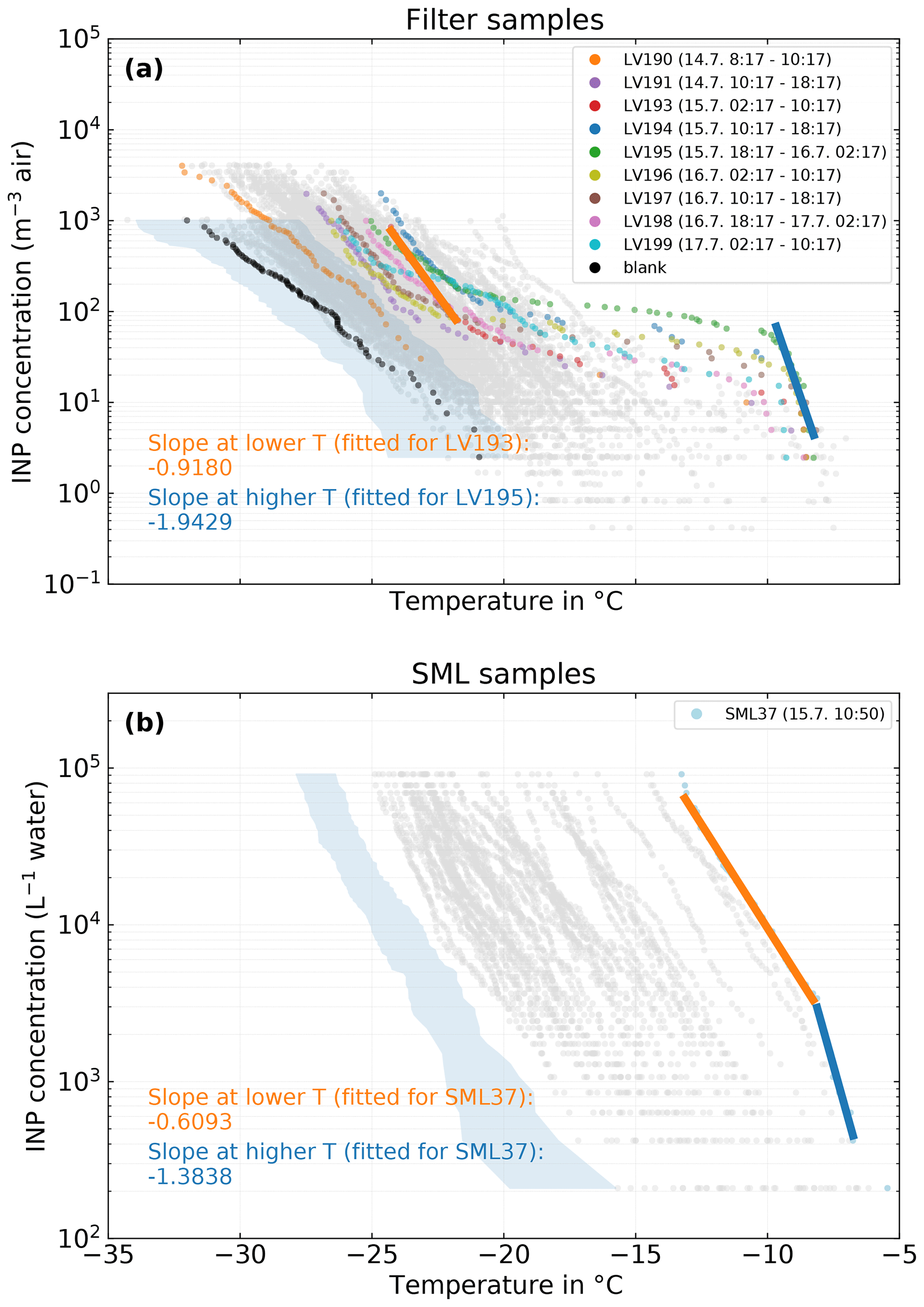
Figure 11(a) Filter samples measured with LINA. Samples that were collected during the period of the case study are shown in color, while all other samples are shown in gray. Exemplary fits for the slopes at lower and higher temperatures for case-study-related samples are shown as orange and blue lines, respectively. The black dots depict the mean freezing spectrum of the field blanks scaled to atmospheric concentrations with the mean sampled air volume of the 8 h filter samples. (b) SML samples measured with INDA. The sample that was collected during the period of the case study is shown in color, while all other samples are shown in gray. As in (a), the fits of the slope are shown as orange and blue lines.

Download

The overall most ice-active SML sample, SML37, was taken on 15 July, 10:50 LT, and is highlighted in Fig. 11 (lower panel, light blue symbols). It occurs at the beginning of the sampling period of LV194, which is the second most ice-active atmospheric filter sample (Fig. 11, upper panel, blue symbols). A number of atmospheric samples collected before and after sample LV194 are also shown. Most of the N_INP(T) spectra from these samples have a very similar overall shape, featuring a fairly steep increase at temperatures above −10 ^∘C, followed by a plateau region between ca. −10 and −21 ^∘C and another but less steep increase below −21 ^∘C. Such a behavior is indicative of the presence of distinct INP populations; therefore, not many mixing events happened during transport (Hartmann et al., 2020a; Welti et al., 2018). Additionally, the INPs active at these warmer temperatures are likely biogenic and proteinaceous as indicated by heat tests described in Sect. 3.1.

Figure 12Aerosol measurements and other relevant parameters during the period of the case study. Shown are (a) the particle number size distribution, (b) the total particle concentrations N_total, (c) cloud concentration nuclei concentration (N_CCN) for 6 different supersaturations, (d) 10 min averages of wind direction and wind speed, (e) chlorophyll a concentration measured by the FerryBox system of Polarstern, and (f) the INP concentration (N_INP) measured with SPIN at different temperatures (color coded). The arrows in panel (b) indicate where total particle concentrations are higher than the axis limit. The colored shaded areas mark the periods where the filter samples were collected. The respective sample ID is shown on top. The black vertical line marks the collection time of the SML sample SML37.

Download

Temperature range and slope of, for example, the initial increase in the temperature spectra are somewhat characteristic for the INPs prevailing. In other words, similar slopes in similar temperature ranges observed for atmospheric and SML samples could be indicative of similar INPs being present in both compartments (Knackstedt et al., 2018). As shown in Fig. 11, the slope of the atmospheric samples at $T>-\mathrm{10}$ ^∘C (linear fit on logarithmic axis) is −1.94, while the slope of the SML sample at $T>-\mathrm{8.2}$ ^∘C is −1.38. The difference in these slopes is too large to unambiguously attribute both samples to the same INP species and too small to reject the possibility. In other words, the similarities in the spectra (temperature range and slopes) at the high freezing temperatures do not prove but can be taken as a hint at similar INPs being present in both the atmosphere and the SML. It is also apparent that the less steep slope at lower temperatures ($T<-\mathrm{8.2}$ ^∘C) of that SML sample has no counterpart in the atmospheric samples. If the atmospheric INPs active above −10 ^∘C would originate from the ocean, this suggests that the aerosolization process might be different for different INP species. Furthermore, it is possible that the INP flux is the other way around, i.e., INPs from the atmosphere are deposited into the SML. However this is highly speculative and needs further research.

To further elucidate the possible connection between atmospheric INPs and INPs in the SML, in the following we consider additionally available aerosol-related and meteorological information.

The highly ice-active sample discussed above, SML37, was taken during a period (approx. 14 July 18:00 to 15 July 19:30) which, as can be seen in Fig. 12, was characterized by a monomodal particle size distribution and, compared to the periods before and after, increased total particle number (N_total, panel b) and CCN (N_CCN, panel c) concentrations. In panel (d) it can be seen that during this period the wind speed decreased significantly, and the wind direction changed slowly from around 240 to 175^∘. Furthermore, during the collection times of the filter samples LV194 and LV195, increased chlorophyll a concentrations were measured by the vessel's FerryBox system (panel e). The elevated chlorophyll a concentrations may indicate enhanced biological activity like a phytoplankton bloom in the vicinity of the vessel during the collection time of the samples LV194 and LV195. Interestingly the chlorophyll a concentration of the highly ice-active sample SML37 itself is not unusually high (0.24 µg L⁻¹; Bracher, 2019). This may have two main reasons. Firstly, while chlorophyll a is an indicator for biological activity, not all marine microorganisms contain chlorophyll a. Secondly, since chlorophyll a itself is not the INP, a correlation is not necessarily to be expected. Also as described in Zeppenfeld et al. (2019) and the references within, the release of ice-active algal exudates may be a feature of decaying plankton blooms. Hence the peak in biological activity, indicated by the chlorophyll a concentration, may be already over, when the peak concentration of ice-active substances occurs. Lastly, panel (f) in Fig. 12 shows N_INP measured with SPIN. Similar to the filter-derived N_INP, also the INP measurements with SPIN remain fairly constant during the period of the case study, and no correlation with the other parameters shown in Fig. 12 can be seen.

To broaden the perspective beyond the aforementioned measurements at the position of the ship itself, HYSPLIT back-trajectories were also assessed.

Figure 13Hourly 3 d back-trajectories (50 m arrival height) for the collection time of the filter samples LV190 to LV199. The color code shows to which sample the trajectory belongs (consistent with Figs. 11 and 12). The Special Sensor Microwave Imager/Sounder (SSMIS) sea ice concentration with emphasized ice edge on 15 July 2017 is also shown (sea ice concentration product of the EUMETSAT Ocean and Sea Ice Satellite Application Facility).

In Fig. 13 the hourly 3 d back-trajectories (50 m arrival height) for the entire period depicted in Fig. 12 are shown. The color code indicates into which collection time, i.e., sample, the respective trajectories fall (corresponding to background colors used in Fig. 12). The trajectories can be categorized into four clusters. The first cluster consists of the trajectories belonging to the samples LV190 and LV191 (orange and purple). These trajectories travel mostly over the ice pack north of Svalbard and have no connection to land. The second cluster comprises the samples LV193, LV194, and LV195 (red, blue, and green), for which the air masses were at the east coast of Greenland before traveling along the ice edge and south of or over Svalbard, before reaching the ship. While CCN and INP number concentrations were elevated during the phase indicated by the red and blue trajectories, the phase connected to the green trajectory coincides with a strong lowering of CCN but still high INP concentrations. The third cluster, which consists of the samples LV197 and LV198 (yellow and brown), came from the same direction as the second cluster but made an additional loop towards the east and back, for which it took about 1 d. For these, N_INP were still high, with medium high concentrations of N_CCN and N_tot during the yellow phase. Unfortunately, aerosol characterization measurements were no longer continued after that time. The trajectories of the fourth cluster (LV198 and LV199; pink and cyan) come from the south and had contact with the Norwegian coast 1–2 d prior to their arrival at Polarstern. Additionally, Fig. S5 in the Supplement shows a map of the wider investigation area together with satellite measurements of chlorophyll a concentrations and the back-trajectories, where it can be seen that biological activity can be found in the region.

While it is a reasonable assumption that the INPs are produced in situ by biological processes, a recent publication by Cornwell et al. (2020) presents a different pathway. They show in a laboratory study that mineral dust deposited in seawater can be re-aerosolized and add to the atmospheric INP population. This pathway is especially interesting as a pathway, because in proximity to the coast meltwater streams can transport dust into the ocean. Pfirman et al. (1989) also describe that sea ice often contains dust particles that can originate from atmospheric deposition or from shelf or shore-fast sea ice which may be transported away from the coast. And as Tobo et al. (2019) observed, dust can also be the carrier for highly ice-active biogenic material; therefore, these dust-related processes may also explain spatially confined areas of high ice activity without being contradictory to the assumption of biogenic INP.

Summarizing and interpreting our observations, the following can be stated:

• The freezing spectra of atmospheric INPs are similar in shape, i.e., a steep slope at warm temperatures followed by an extended plateau region followed by less steep slope, indicating that during the case study similar atmospheric INP populations were sampled.

• Heat tests indicate that INPs active above −15 ^∘C are biogenic and proteinaceous.

• The freezing spectra of atmospheric INPs and INPs from the SML feature similar slopes at temperatures above −10 ^∘C, suggesting a connection between both compartments, which, however, as discussed above, would need a substantial enrichment of INPs during the sea spray production.

• Aerosol particle parameters show that clearly different air masses arrive at Polarstern over the course of the case study.

• Back-trajectories indicate that sampled air masses have different regions of origin and travel over different pathways towards Polarstern.

• Elevated chlorophyll a concentrations were observed for a short phase directly at the position of Polarstern (FerryBox) and also in the wider geographical region in the week-long satellite composite. This indicates a high biological activity in the investigation region.

We interpret these findings as strong indication for a local marine source being present during our case study. Seemingly this is in contradiction to the results gained from the analysis of fog water as presented above, unless a significant enrichment of INPs takes place during the aerosolization of seawater and/or SML material. In other words, there is a strong need for gaining knowledge concerning the mechanisms of aerosolization and resulting fluxes of INPs and related species at the ocean–atmosphere interface.