A study of the dynamical characteristics of inertia–gravity waves in the Antarctic mesosphere combining the PANSY radar and a non-hydrostatic general circulation model

Shibuya, Ryosuke; Sato, Kaoru

doi:https://doi.org/10.5194/acp-19-3395-2019

Articles | Volume 19, issue 5

https://doi.org/10.5194/acp-19-3395-2019

Articles | Volume 19, issue 5

Research article

18 Mar 2019

Research article |

| 18 Mar 2019

A study of the dynamical characteristics of inertia–gravity waves in the Antarctic mesosphere combining the PANSY radar and a non-hydrostatic general circulation model

Ryosuke Shibuya and Kaoru Sato

Abstract

This study aims to examine the dynamical characteristics of gravity waves with relatively low frequency in the Antarctic mesosphere via the first long-term simulation using a high-top high-resolution non-hydrostatic general circulation model (NICAM). Successive runs lasting 7 days are performed using initial conditions from the MERRA reanalysis data with an overlap of 2 days between consecutive runs in the period from April to August in 2016. The data for the analyses were compiled from the last 5 days of each run. The simulated wind fields were closely compared to the MERRA reanalysis data and to the observational data collected by a complete PANSY (Program of the Antarctic Syowa MST/IS radar) radar system installed at Syowa Station (39.6^∘ E, 69.0^∘ S). It is shown that the NICAM mesospheric wind fields are realistic, even though the amplitudes of the wind disturbances appear to be larger than those from the radar observations.

The power spectrum of the meridional wind fluctuations at a height of 70 km has an isolated and broad peak at frequencies slightly lower than the inertial frequency, f, for latitudes from 30 to 75^∘ S, while another isolated peak is observed at frequencies of approximately 2π∕8 h at latitudes from 78 to 90^∘ S. The spectrum of the vertical fluxes of the zonal momentum also has an isolated peak at frequencies slightly lower than f at latitudes from 30 to 75^∘ S at a height of 70 km. It is shown that these isolated peaks are primarily composed of gravity waves with horizontal wavelengths of more than 1000 km. The latitude–height structure of the momentum fluxes indicates that the isolated peaks at frequencies slightly lower than f originate from two branches of gravity wave propagation paths. It is thought that one branch originates from 75^∘ S due to topographic gravity waves generated over the Antarctic Peninsula and its coast, while more than 80 % of the other branch originates from 45^∘ S and includes contributions by non-orographic gravity waves. The existence of isolated peaks in the high-latitude region in the mesosphere is likely explained by the poleward propagation of quasi-inertia–gravity waves and by the accumulation of wave energies near the inertial frequency at each latitude.

Download & links

Article (PDF, 12137 KB)

Supplement (249 KB)

Download & links

Article (12137 KB)
Supplement (249 KB)
BibTeX
EndNote

How to cite

How to cite.

Dates

Received: 27 Sep 2018 – Discussion started: 17 Oct 2018 – Revised: 15 Jan 2019 – Accepted: 08 Mar 2019 – Published: 18 Mar 2019

1 Introduction

Waves propagating in the stably stratified atmosphere with buoyancy as a restoring force are traditionally called gravity waves. Gravity waves transport momentum upward from the troposphere to the middle atmosphere and are recognized as a major driving force for large-scale meridional circulation in the middle atmosphere (e.g., Fritts and Alexander, 2003). Because the horizontal wavelengths of significant parts of gravity waves are shorter than several hundreds of kilometers, many climate models use parameterization methods to calculate momentum deposition via unresolved gravity waves (e.g., McFarlane, 1987; Scinocca, 2003; Richter et al., 2010). Currently, many gravity wave parameterizations are based on very simple assumptions related to essential wave dynamics, such as source spectra and propagation properties. Even though physically based gravity wave parameterizations have recently been developed (e.g., Beres et al., 2004; Song and Chun, 2005; Cámara et al., 2014; Charron and Manzini, 2002; Richter et al., 2010), tuning parameters, which are ill-defined in general circulation models, such as the moving speeds of sub-grid convective cells related to the phase speeds of launched gravity waves (Beres et al., 2004; Choi and Chun, 2011) or the occurrence rate for wave launching for the frontogenesis function (Richter et al., 2010), still exist.

Geller et al. (2013) showed that parameterized gravity waves in climate models are not realistic in several aspects, particularly at high latitude, compared to high-resolution observations and high-resolution general circulation models. Such improper specifications of gravity wave momentum deposition by parameterizations are thought to lead to several serious problems, such as the so-called cold-pole bias problem (SPARC, 2010; McLandress et al., 2012; Garcia et al., 2017). However, many previous studies have suggested that the Antarctic region has multiple types of gravity wave sources, such as the mountains of the southern Andes and the Antarctic Peninsula (e.g., Eckermann and Preusse, 1999; Alexander and Teitelbaum, 2007; Sato et al., 2012), the small islands around the Southern Ocean (Wu et al., 2006; Alexander et al., 2010; Hoffmann et al., 2013), the leeward propagation of gravity waves from lower and high latitudes (Sato et al., 2009, 2012; Hindley et al., 2015), the upper tropospheric jet stream (Shibuya et al., 2015; Jewtoukoff et al., 2015), and the strong polar night jet (Yoshiki and Sato, 2000; Sato and Yoshiki, 2008; Sato et al., 2012). Therefore, these processes may frequently overlap in time and space, suggesting that process-based analyses based on observational data are unavoidable. In response to such recognitions of the importance of gravity waves in the Antarctic, several observational campaigns in the lower stratosphere have been conducted (e.g., VORCORE, Hertzog et al., 2008; CONCORDIASI, Rabier et al., 2010; DEEPWAVE, Fritts et al., 2016).

Due to the harsh environment in the Antarctic, it is still challenging to perform observation of the mesosphere. Previous studies have used several observational instruments at limited ground-based observation sites, such as medium-frequency (MF) radar (e.g., Dowdy et al., 2007), meteor radar (Tsutsumi et al., 1994; Forbes et al., 1995), metal fluorescence lidar (e.g., Gardner et al., 1993; Arnold and She, 2003; Chen et al., 2016), and airglow imagers (e.g., Garcia et al., 2000; Matsuda et al., 2014). Using these instruments, these studies have primarily focused on the temporal–spatial structures of migrating and non-migrating tides using observational data at one or a couple Antarctic stations (e.g., Murphy et al., 2006, 2009; Hibbins et al., 2010) and the generation and propagation mechanisms of tides using numerical models (e.g., Aso, 2007; Talaat and Mayr, 2011). However, the dominant vertical wavenumbers of gravity waves have rarely been examined due to the coarse vertical resolution of the MF radars. Moreover, due to the limited number of Antarctic stations, it is still very difficult to examine the spatial structures of gravity waves observed in the mesosphere. Therefore, discussions concerning the dynamics of gravity waves in previous studies have been based on results from frequency spectrum analyses of the horizontal winds (e.g., Kovalam and Vincent, 2003) or from variance analyses of gravity wave wind fluctuations and their seasonal (e.g., Hibbins et al., 2007) and interannual (e.g., Yasui et al., 2016) variations. Even though a few studies using ground-based observations attempted to estimate the sources of the observed mesospheric gravity waves using heuristic ray tracing methods (e.g., Nicolls et al., 2010; Chen et al., 2013), a statistical analysis is required to understand the dynamical characteristics of mesospheric gravity waves.

Observational instruments on board satellites have also been used to detect the spatial distributions of temperature (radiance) data in the mesosphere (MLS: Wu and Waters, 1996; Jiang et al., 2005; CRISTA: Preusse et al., 2006; SABER: Preusse et al., 2009; Yamashita et al., 2013). In addition, the momentum flux of mesospheric gravity waves is estimated using the SABER temperature data (Ern et al., 2018). However, the variances and momentum fluxes estimated from satellite data contain contributions from a limited portion of the gravity wave spectrum due to the observational filtering effects of each satellite instrument (e.g., Alexander et al., 2010).

To examine the dynamical characteristics of gravity waves, high-resolution general circulation models that directly resolve a relatively wide range of the gravity wave spectrum are powerful tools. At present, however, only four models have been used to directly resolve mesospheric gravity waves with minimal resolved horizontal wavelengths (λ_min) of less than 400 km and with fine vertical resolutions (dz) of less than 600 m in the middle atmosphere. Becker (2009) used the Kühlungsborn Mechanistic General Circulation Model (KMCM) to examine the sensitivity of the state of the upper mesosphere to the strength of the Lorenz energy cycle in the troposphere. Zülicke and Becker (2013) used KMCM to examine the dynamical responses of the mesosphere to a stratospheric sudden warming (SSW) event. In addition, by combining KMCM simulations and MF radar observations in the Northern Hemisphere, Hoffman et al. (2010) explored the relationship between the activities of mesospheric gravity waves and critical level filtering via background wind. Liu et al. (2014) used the mesosphere-resolving version of the Whole Atmosphere Community Climate Model to create a horizontal map of mesospheric perturbations such as concentric gravity waves, which are likely excited by deep convection in the low to middle latitudes. The KANTO model (Watanabe et al., 2008) is based on the atmospheric component of version 3.2 of the Model for Interdisciplinary Research on Climate (MIROC; K-1 Model Developers, 2004; Nozawa et al., 2007). Sato et al. (2009) used KANTO to discuss the dominant sources of mesospheric gravity waves using characteristics of the 3-D momentum flux distribution. Tomikawa et al. (2012) examined the dynamical mechanism of an elevated stratopause event associated with an SSW event that spontaneously occurred in the KANTO model. Last, the JAGUAR model is the KANTO model with the model top extended to z_top≅150 km including nonlocal thermodynamic equilibrium (non-LTE) for infrared radiation processes. Using JAGUAR, Watanabe and Miyahara (2009) examined the dynamical relationship between migrating tides and gravity wave forcing at low latitudes. Note that all the current models permitting mesospheric gravity waves described above are hydrostatic general circulation models.

As mentioned above, a few studies have focused on the dynamical characteristics of gravity waves, such as their propagation and/or generation processes in the Antarctic mesosphere. However, no study has attempted to simulate mesospheric gravity waves whose reality is confirmed via high-resolution observations for a long time period. This is partially because there are few observational instruments with a sufficiently high resolution to validate mesospheric gravity waves simulated in models. Therefore, the dynamical characteristics of gravity waves observed in the Antarctic mesosphere have not been fully examined using both observations and numerical simulations.

This study uses two novel methods. One is the first Mesosphere–Stratosphere–Troposphere/Incoherent Scattering (MST/IS) radar in the Antarctic, which was recently installed at Syowa Station (39.6^∘ E, 69.0^∘ S) by the “Program of the Antarctic Syowa MST/IS radar” project (the PANSY radar; Sato et al., 2014). The PANSY radar is capable of capturing the fine vertical structures of horizontal and vertical mesospheric wind disturbances when the mesosphere is ionized, primarily by solar radiation during the daytime. Such a high resolution is unique in the Antarctic. This means that the observational data from the PANSY radar can be used to validate the results of models permitting mesospheric gravity waves at fine vertical resolution. Furthermore, this study uses the high-top version (Shibuya et al., 2017) of the Non-hydrostatic Icosahedral Atmospheric Model (NICAM; Satoh et al., 2014). This is a global cloud-resolving model with a non-hydrostatic dynamical core with icosahedral grids. Such a non-hydrostatic model is likely preferable for simulations of the high-intrinsic-frequency gravity waves contributing to a large portion of the momentum flux convergence in the upper-middle atmosphere (e.g., Reid and Vincent, 1987; Fritts and Vincent, 1987; Fritts, 2000; Sato et al., 2017). Moreover, gravity waves generated by deep convection are expected to be correctly resolved in non-hydrostatic models.

Recently, using continuous PANSY radar observations of polar mesosphere summer echoes (PMWEs) at heights from 81 to 93 km, Sato et al. (2017) showed that relatively low-frequency disturbances from 1 day⁻¹ to 1 h⁻¹ primarily contribute to the zonal and meridional momentum fluxes. This study examines the dynamical characteristics of gravity waves with relatively low frequency in the Antarctic mesosphere, such as the wave parameters, propagation, and generation mechanisms, via a long-term simulation using the high-top high-resolution non-hydrostatic general circulation model for 5 months from April to August in 2016. The simulated wind fields are closely compared to the PANSY radar observations at small scales and the MERRA reanalysis data at large scales. In addition, the statistical characteristics of the mesospheric disturbances simulated by NICAM, such as the frequency (ω) spectra of each variable, the kinetic and potential energies, and the momentum and energy fluxes of the gravity waves, are examined.

This paper is organized as follows. The methodology is described in Sect. 2. The numerical results are compared to the observational results in Sect. 3. The gravity wave characteristics are examined based on a spectrum analysis in Sect. 4. A discussion is presented in Sect. 5, and Sect. 6 summarizes the results and provides concluding remarks.

2 Methodology

2.1 The PANSY radar observations

The PANSY radar is the first MST/IS radar in the Antarctic and is installed at Syowa Station (39.6^∘ E, 69.0^∘ S) to observe the Antarctic atmosphere in the height range from 1.5 to 500 km. Note that an observational gap exists from 25 to 60 km due to the lack of backscatter echoes in this height region (Sato et al., 2014). The PANSY radar employs a pulse-modulated monostatic Doppler radar system with an active phased array consisting of 1045 crossed-Yagi antennas. The PANSY radar observations of the 3-D winds have standard time and height resolutions along the beam direction of $Δ t = \sim 1$ min and Δz=150 m for the troposphere and lower stratosphere and $Δ t = \sim 1$ min and Δz=300–600 m for the mesosphere. The accuracy of the line-of-sight wind velocity is approximately 0.1 m s⁻¹. Because the target of the MST radars is the atmospheric turbulence, wind measurements can be made under all weather conditions. Continuous observations have been made by a partial PANSY radar system since 30 April 2012 and by a full system since October 2015. See Sato et al. (2014) for further details concerning the PANSY radar system.

The PANSY radar data that we use are line-of-sight wind velocities of five vertical beams in the vertical direction and tilted east, west, north, and south at a zenith angle of θ=10^∘ for the period of April–May 2016, during which the PANSY radar frequently detects the PMWEs at heights of 60–80 km (Nishiyama et al., 2015). The vertical wind component is directly estimated from the vertical beam. The zonal wind component is obtained using a pair of line-of-sight velocities from the east and west beams. The line-of-sight velocities of the east and west beams, V_±θ, are composed of the zonal and vertical components of the wind velocity $(u_{\pm θ}, w_{\pm θ})$ in a targeted volume range:

V_{\pm θ} = \pm u_{\pm θ} \sin θ + w_{\pm θ} \cos θ .

Assuming that the wind field is homogeneous at each height, i.e., $u_{+ θ} = u_{- θ} \equiv u$ and $w_{+ θ} = w_{- θ} \equiv w$ , we can estimate the zonal wind component as

u = \frac{V_{+ θ} - V_{- θ}}{2 \sin θ} .

The meridional wind component is estimated in the same way using the north and south beams.

2.2 Numerical setup for the non-hydrostatic model simulation

The simulation was performed using the NICAM, which is a global cloud-resolving model (Satoh et al., 2008, 2014). The non-hydrostatic dynamical core of the NICAM was developed using icosahedral grids modified via the spring dynamics method (Tomita et al., 2002). The simulation period is from 20 March to 31 August 2016.

2.2.1 Grid coordinate system and physical schemes

The resolution of the horizontal icosahedral grids is represented by g-level n (grid-division-level n). G-level 0 denotes the original icosahedron. By recursively dividing each triangle into four smaller triangles, a higher resolution is obtained. The total number of grid points is $N_{g} = 10 \cdot 4^{n} + 2$ for g-level n. The actual resolution corresponds to the square root of the averaged control volume area, $Δ x \equiv \sqrt{4 π R_{E}^{2}} / N_{g}$ , where R_E is the Earth's radius. A grid with g-level 8 is used in this study (Δx∼28 km).

Recently, Shibuya et al. (2016) developed a new icosahedral grid configuration that has a quasi-uniform and regionally fine mesh within a circular region using spring dynamics. This method clusters grid points over a sphere into a circular region (the target region). By introducing sets of mathematical constraints, it has been shown that the minimum resolution within the target region is uniquely determined by the area of the target region. In this study, the target region for a given g-level is a region south of 30^∘ S centered on the South Pole, corresponding to a horizontal resolution of approximately 18 km in the target region.

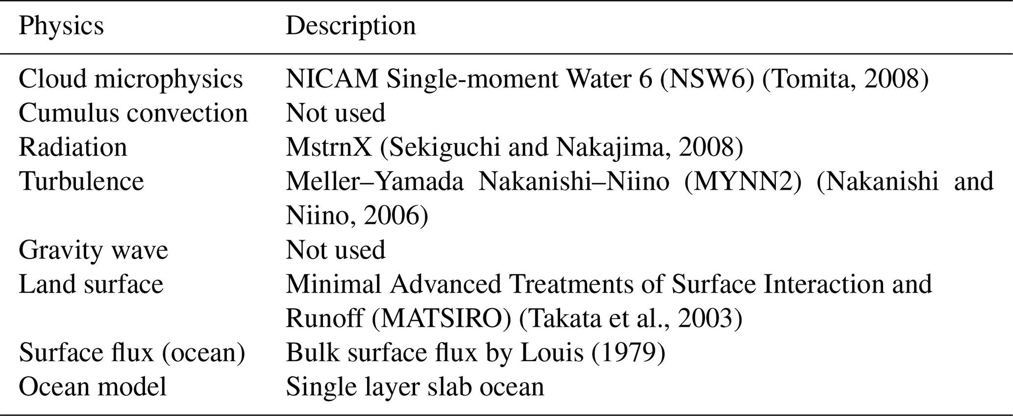
In order to adequately simulate the structures of the disturbances in the stratosphere and the mesosphere, the vertical grid spacing is set to 300 m at heights from 2.4 to 80 km. Note that, according to Watanabe et al. (2015), the gravity wave momentum flux is not heavily dependent on the vertical spacing of the model in the middle atmosphere when Δz<400 m. The number of vertical grids is 288. To prevent unphysical wave reflections at the top of the boundary, a 7 km thick sponge layer is set above z=80 km. Second-order Laplacian horizontal hyperviscosity diffusion and Rayleigh damping for the vertical velocity are used in the sponge layer. The e-folding time of the ∇² horizontal diffusion for a 2Δx wave at the top of the model is 4 s, and the e-folding time of Rayleigh damping for the vertical velocity at the top of the model is 216 s. The diffusivity level gradually increases from the bottom to the top of the sponge layer. We confirmed that little wave reflection near the sponge layer occurs under this setting (not shown). In addition, to prevent numerical instabilities in the model domain, sixth-order Laplacian horizontal hyperviscosity diffusion is used over the entire height region. The e-folding time of the ∇⁶ horizontal diffusion for a 2Δx wave at the top of the model is approximately 2 s. As a result, the high-top NICAM model can resolve gravity waves with horizontal wavelengths longer than approximately 250 km. Table 1 summarizes the physical schemes used in this study. No cumulus or gravity wave parameterizations were employed. Note that this model does not use the nudging method as an external forcing for the atmospheric component.

Table 1Physics scheme used in the high-top NICAM.

Download Print Version | Download XLSX

2.2.2 Initial condition and time integration technique

MERRA reanalysis data based on the Goddard Earth Observing System Data Analysis System, Version 5 (GEOS-5 DAS; Rienecker et al., 2011) is used as the initial condition for the atmosphere. The initial data for the land surface and slab ocean models were interpolated from the 1.0^∘ gridded National Centers for Environmental Prediction final analysis. In the MERRA reanalysis data, the following two types of 3-D fields are provided: one is produced using the corrector segment of the incremental analysis update (IAU; Bloom et al., 1996) cycle ( $1.25^{\circ} \times 1.25^{\circ}$ with 42 vertical levels whose top is 0.1 hPa) and the other pertains to fields resulting from the grid point statistical interpolation analyses (GSI analysis; e.g., Wu et al., 2002) on a native horizontal grid with native model vertical levels ( $0.75^{\circ} \times 0.75^{\circ}$ with 72 vertical levels whose top is 0.01 hPa). We use the former 3-D assimilated fields from 1000 to 0.1 hPa and the latter 3-D analyzed fields from 0.1 to 0.01 hPa for the initial conditions of the NICAM simulation to prepare realistic atmospheric fields in the mesosphere. The latter 3-D analyzed fields were only used at heights above 0.1 hPa because variables for the vertical pressure velocity, cloud liquid water, and ice mixing ratios are not included and thus have been set to zero. The vertical pressure velocities, cloud liquid water, and ice mixing ratios above 0.1 hPa were set to zero. The time step was 15 s, and the model output was recorded every hour. Note that the satellite observation data related to the stratospheric temperature profiles are provided up to 50 km the data assimilation technique is only applied below the height (Sakazaki et al., 2012).

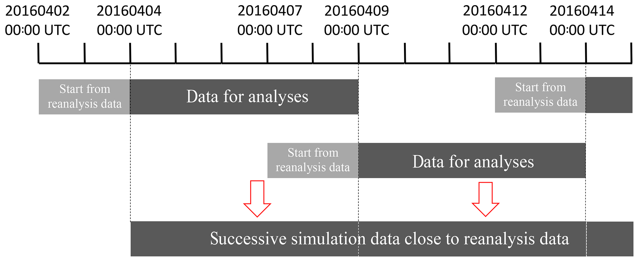
Time integrations were performed following a technique similar to Plougonven et al. (2013) to maintain long-term simulations sufficiently close to the reanalysis data. The time integration method is illustrated in Fig. 1. Simulations lasted 7 days for each run with initial conditions from the MERRA reanalysis data with an overlap of 2 days between each run. The 2-day overlap consists of the spin-up time for the subsequent simulation. The successive data for the analyses were compiled using the data from the last 5 days of each run. This method allows the model to freely produce gravity waves and mesoscale phenomena without artifacts caused by nudging and assimilation techniques. However, because the successive simulation data are not continuous, spurious and drastic jumps in the atmospheric fields between two consecutive simulations may appear. Therefore, in this study, the statistical analyses are performed by taking an average of the results using the respective 5-day simulations to avoid any influences from gaps between the simulations. A long-term continuous run from a single initial condition was not performed because the model fields tend to diverge from the actual atmosphere without appropriate parameterization methods and/or nudging or assimilation techniques.

https://www.atmos-chem-phys.net/19/3395/2019/acp-19-3395-2019-f01

Figure 1An illustration for the time integration method.

Download

3 Results and comparisons of the numerical simulations

3.1 Wave structures in the mesosphere

Figure 2 shows time–height sections of the line-of-sight winds observed by the north beam of the PANSY radar and V_N calculated using v and w simulated by NICAM for 10–20 May 2016 ( $V_{N} = v \sin θ + w \cos θ$ , where θ=10^∘). The missing values in the PANSY radar observation are shown in white. The black dotted vertical lines in Fig. 2b indicate the segments of the continuous 5-day simulations. In the middle of May, large amounts of observational data from the PANSY radar are available because strong PMWEs were observed in the daytime during this period.

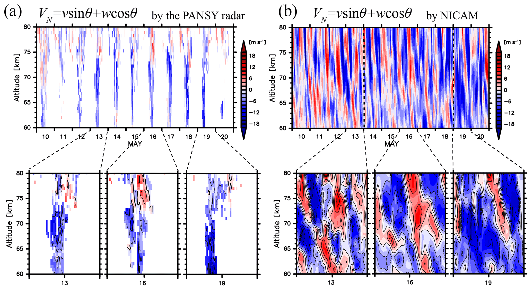
https://www.atmos-chem-phys.net/19/3395/2019/acp-19-3395-2019-f02

Figure 2Time–altitude cross sections of northward line-of-sight speeds (a) observed by the PANSY radar at Syowa Station (a) for the period from 10 to 20 May 2015 and (b) those simulated by NICAM in the same period. The contour intervals are 4 m s⁻¹. The black dotted vertical lines in panel (b) denote the segments of the lasting 5-day simulation.

Download

At heights of 60–75 km, negative V_N values are dominant during the observed periods, which is consistent with the direction of the mesospheric residual circulation in the winter hemisphere. On 13 and 16 May it appears that disturbances with negative vertical phase speeds are dominant in the height range of 75–80 km. These features are also observed in the model data in Fig. 2b. The downward-propagating disturbances have positive V_N values at heights of 75–80 km on 13 and 16 May as in Fig. 2a. Therefore, the overall wave structures are well reproduced by NICAM. However, the phases of the disturbances on 13 May, which is the final day of the 7-day integration from the initial condition, are different from the observations. The possible reason for this is that the propagation path of the wave packet simulated in NICAM on 13 May may be unrealistic since the large-scale fields likely do not remain sufficiently close to the reanalysis data after such a long simulation time.

To quantitatively compare the wave structures observed by the PANSY radar and those simulated by NICAM, the amplitudes of the wave disturbances were estimated as a function of the vertical phase velocities. Figure 3a and b show time–height sections of the line-of-sight winds observed by the north beam of the PANSY radar for 26–28 April and a close-up for 28 April 2016, respectively.

https://www.atmos-chem-phys.net/19/3395/2019/acp-19-3395-2019-f03

Figure 3Time–altitude cross sections of northward line-of-sight speeds (a) observed by the PANSY radar for the period from (a) 24 to 26 April 2016 and (b) 26 April 2016. (b) Phase lines with a vertical phase velocity of V₁ are denoted as L₁, L₂, ..., L_i, ..., L_N (thick black lines), and data points on L_i are denoted as $x_{1}^{i}$ , $x_{2}^{i}$ , ..., $x_{n_{i}}^{i}$ (black circles). Other phase lines with a vertical phase velocity of V₂ and data points on their phase lines are depicted by red. Please see the text in detail.

Download

The estimation method is illustrated below. Here, phase lines at heights of 65–80 km from 04:00 to 18:00 UTC are defined as L₁, L₂, ..., L_i, ... L_N (denoted by the black lines in Fig. 3b) and sets of data points on L_i ( $x_{1}^{i}$ , $x_{2}^{i}$ , ..., $x_{n_{i}}^{i}$ ; the black circles in Fig. 3b) are defined as M_i ( $x_{1}^{i}$ , $x_{2}^{i}$ , ..., $x_{n_{i}}^{i} \in M_{i}$ ). The estimated amplitude A of disturbances with the vertical phase velocity V₁ is defined by calculating the average of the covariances of $M_{1}, M_{2}, \dots M_{N}$ :

\begin{array}{l} A^{2} = & 2.0 \times [\sum_{k} (\sum_{i \geq j} x_{i}^{k} x_{j}^{k} (i, j \in M_{k})) / \\ (1) & \sum_{k} (\sum_{i \geq j} 1 (i, j \in M_{k}))] \end{array}

When the disturbance is due to a monochromatic wave defined by V₁ ( $ψ = a \cos i (m z - ω t)$ , where $ω / m = V_{1}$ ), the estimated amplitude A is equal to the amplitude of the monochromatic wave a. However, the estimated amplitude A becomes very small when phase lines with the vertical phase velocity do not match the wave structure (V₂, the red lines in Fig. 3b). Therefore, the estimated magnitude A has a peak at the dominant vertical phase velocity of the wave disturbances. In a simple case with cos iπ(2t−z), a result of the estimation by the method is shown as an example in Fig. S1 in the Supplement.

The main advantage of this method is that it can easily be applied to both simulated data and observed data that have missing values, as in the PANSY radar observations. Prior to the application of this method, a bandpass filter is applied to the observed and simulated northward line-of-sight winds with cutoff wave periods of 2 and 60 h to extract the dominant wave-like structures. In this study, the estimation method for the PANSY radar observation is only applied to data on days for which the ratio of the available data points in a period from 04:00 to 18:00 UTC and at heights of 65–80 km exceeds 60 % (25 and 26 April in Fig. 3a). Here, the PANSY radar observation data in April and May are used for this analysis since large numbers of observational data are available in these months (12 and 16 days, respectively).

Figure 4a and b show the estimated amplitude as a function of the vertical downward phase velocity in April and May using data from the PANSY radar observations and the NICAM simulations, respectively. In Fig. 4a, it appears that the dominant wave disturbances observed by the PANSY radar have vertical phase velocities of approximately 0.5 and 0.7 m s⁻¹ in April and May, respectively. These features are well simulated by the NICAM simulations (Fig. 4b). Therefore, the dominant wave structures in the time–altitude section in the NICAM simulations are likely very similar to those observed by the PANSY radar. However, the mesospheric disturbances simulated by NICAM have an approximately 3.5 times larger amplitude than those observed by the PANSY radar. Using a hodograph analysis, Shibuya et al. (2017) showed that NICAM simulations overestimate wave amplitudes by approximately 1.5 times compared to the PANSY radar observations in the mesosphere. The possible reasons for the overestimation of wave amplitude in NICAM will be discussed in the end of Sect. 5.

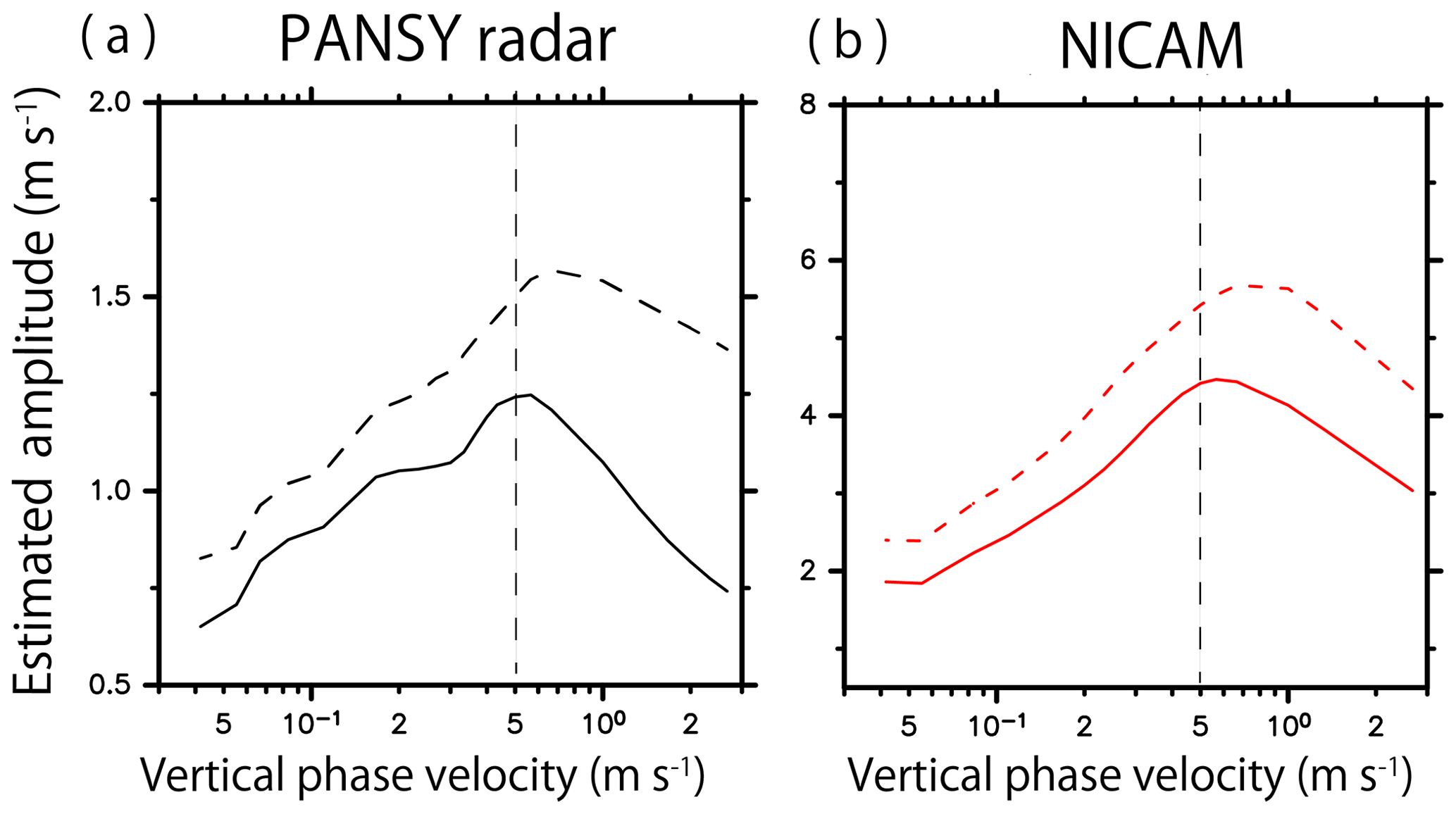
https://www.atmos-chem-phys.net/19/3395/2019/acp-19-3395-2019-f04

Figure 4Estimated wave amplitude as a function of vertical phase velocities in April (black curves) and in May (dashed curves) using (a) the PANSY radar observation and (b) the NICAM simulation.

Download

3.2 Zonal wind components from the troposphere to the mesosphere

Next, zonal wind components simulated by NICAM are compared to those in the MERRA reanalysis data. Figure 5 shows time–altitude cross sections of the zonal winds from the MERRA reanalysis data and from the NICAM simulations for the period of 10–20 May 2016, at a grid near Syowa Station. In Fig. 5b, jumps between the continuous 5-day simulations are observed in the troposphere and the lower stratosphere. This is likely because the large-scale flows diverge from the MERRA reanalysis data during the 7-day integrations. Nevertheless, roughly speaking, the disturbances in the troposphere and lower stratosphere are successfully simulated by NICAM. Conversely, in the upper stratosphere and mesosphere, large-amplitude disturbances with negative vertical phase speeds are clear in the NICAM data but rarely seen in the MERRA reanalysis data. Therefore, to validate the dynamical characteristics of the mesospheric disturbances simulated by NICAM, observational data with high vertical and temporal resolution, such as data from the PANSY radar, are required.

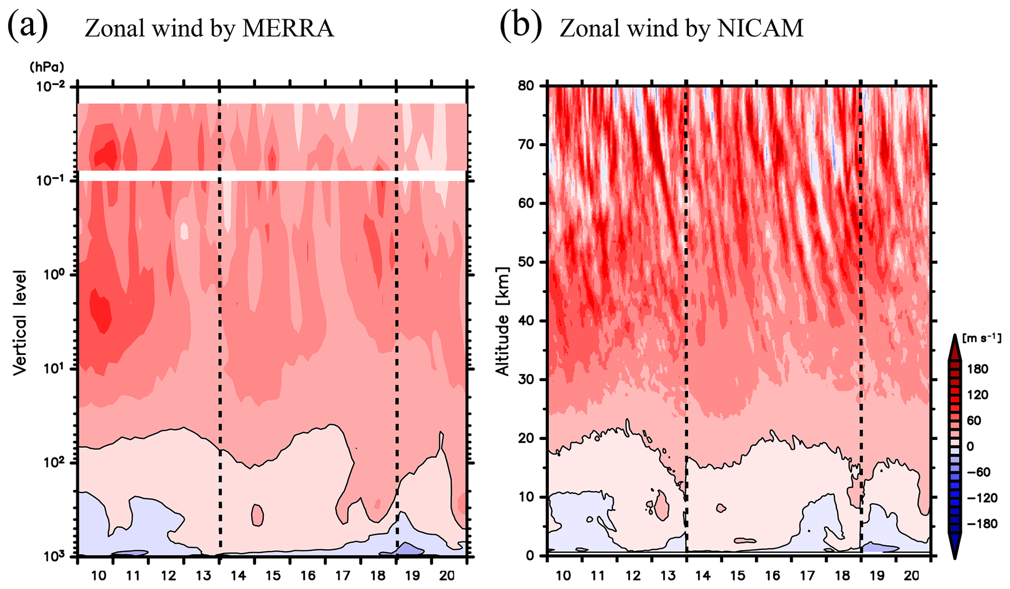
https://www.atmos-chem-phys.net/19/3395/2019/acp-19-3395-2019-f05

Figure 5Time–altitude cross sections of zonal winds (a) from the MERRA reanalysis data and (b) from NICAM simulations for the period from 10 to 20 May 2015 at a grid near Syowa Station. The contour intervals are 20 m s⁻¹. The vertical dotted lines denote the segments of the continuous 5-day simulation by NICAM. (a) The 3-D assimilated fields of the MERRA reanalysis data for 1000 to 0.1 hPa and the 3-D analyzed fields for 0.1 to 0.01 hPa are drawn.

Download

In addition, the latitude–altitude structures of the mean zonal winds averaged in April and May 2016 between the MERRA reanalysis data and the NICAM simulations are compared in Fig. 6. In April and May 2016, it appears that the polar night jet in the upper stratosphere and mesosphere tilts equatorward with height. Such a feature is successfully simulated by NICAM. In particular, the structure of the polar night jet below 35 km in NICAM agrees with that in MERRA. However, the magnitude of the zonal wind around the core of the polar night jet in NICAM is slightly larger than that in MERRA. In addition, the axis of the polar night jet in the mesosphere in NICAM does not tilt as strongly equatorward with height as it does in MERRA. Therefore, the zonal momentum balance in the mesosphere at the initial conditions is not completely maintained in NICAM, likely due to unresolved gravity waves with short horizontal wavelengths. Even though some discrepancies are observed in the mesosphere, the structure of the polar night jet in NICAM is sufficiently close to that in MERRA. Hereafter, analyses of the gravity wave characteristics are performed using data for the time period of 1 June–31 August 2016 (JJA).

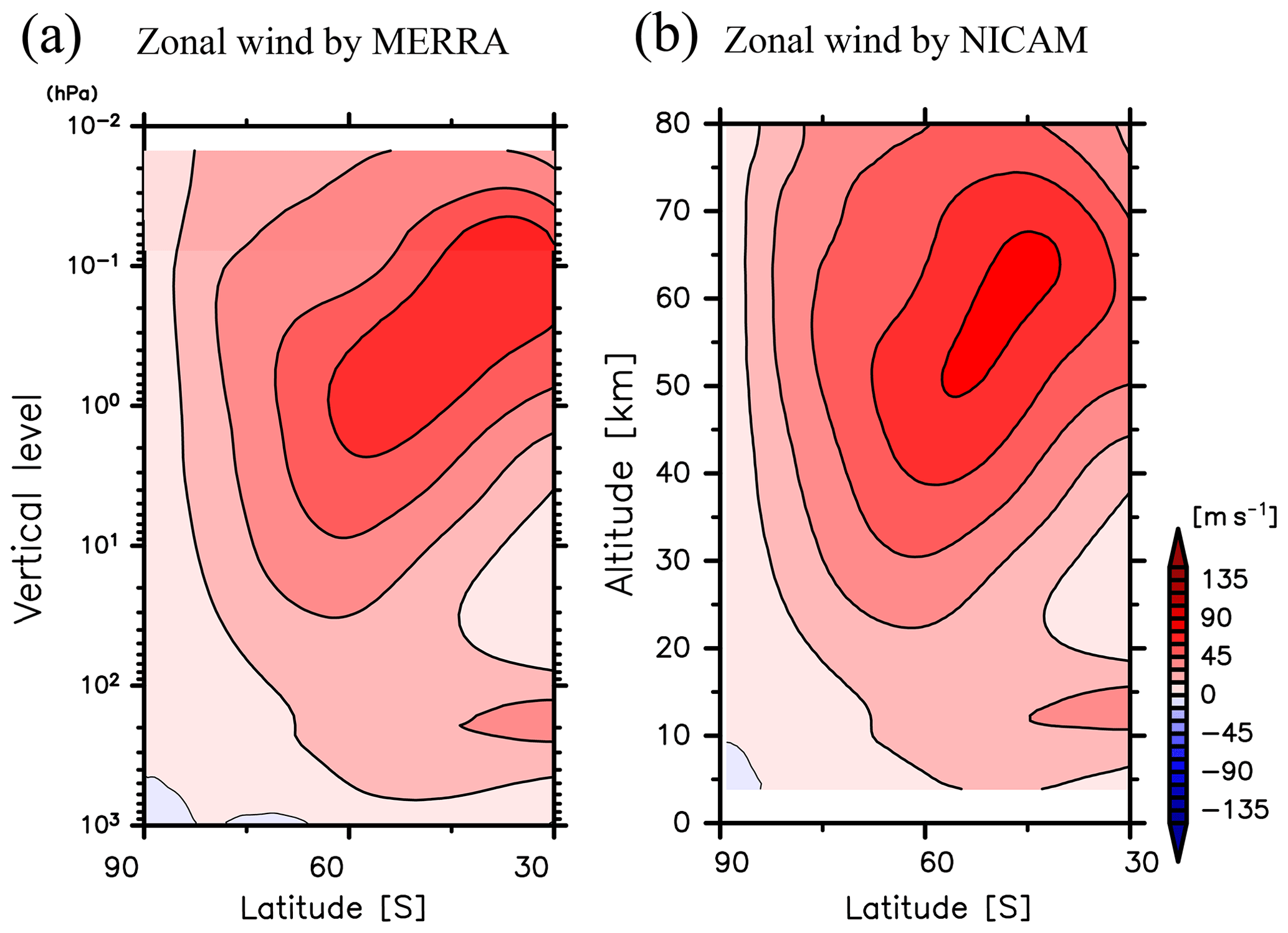
https://www.atmos-chem-phys.net/19/3395/2019/acp-19-3395-2019-f06

Figure 6Latitude-altitude cross sections of the zonal mean zonal winds (a) from MERRA and (b) from NICAM simulations averaged in April and May 2016. The contour intervals are 20 m s⁻¹.

Download

4 Gravity wave characteristics in the mesosphere

4.1 Gravity wave energy and momentum fluxes

In this subsection, the spatial structures of the kinetic and potential energies and the momentum and energy fluxes of the gravity waves are examined. The gravity wave component is defined as wave components with frequencies higher than 2π∕30 h. Note that previous studies have defined the planetary wave component to have frequencies lower than approximately 2π∕40 h in the mesosphere (e.g., Murphy et al., 2007; Baumgaertner et al., 2008).

In the linear theory of inertia–gravity waves,

\begin{array}{l} (u^{'}, v^{'}, w^{'}, \frac{p^{'}}{\overline{p}}, \frac{ρ^{'}}{\overline{ρ}}, \frac{θ^{'}}{\overline{θ}}) = \\ (2) & (\tilde{u}, \tilde{v}, \tilde{w}, \tilde{p}, \tilde{ρ}, \tilde{θ}) \exp i (k x + l y + m z - ω t), \end{array}

where ∼ denotes the Fourier transform of each variable and ω denotes the ground-based frequency. The polarization relations for the different variables are written as

\begin{array}{l} \tilde{u} = (\frac{i \hat{ω} k - f l}{i \hat{ω} l + f k}) \tilde{v} \\ (3) & \tilde{p} = (\frac{{\hat{ω}}^{2} - f^{2}}{\hat{ω} k + i f l}) \tilde{u} \end{array}

and

\tilde{w} = - \frac{m \hat{ω}}{N^{2} - {\hat{ω}}^{2}} \tilde{p},

where $\hat{ω}$ denotes the inertial frequency of gravity waves given by

\begin{matrix} (4) & \hat{ω} = ω - U \cdot k . \end{matrix}

Using these relations, the real component of the zonal and meridional components of the vertical momentum flux $(\overline{u^{'} w^{'}}, \overline{v^{'} w^{'}})$ and that of the horizontal momentum flux ( $\overline{u^{'} v^{'}}$ ) are expressed as

(\overline{u^{'} w^{'}}, \overline{v^{'} w^{'}}) = - \frac{N^{2} - {\hat{ω}}^{2}}{{\hat{ω}}^{2} - f^{2}} \cdot \frac{1}{m} (k, l) \cdot {\overline{w}}^{' 2}

and

\begin{matrix} (5) & \overline{u^{'} v^{'}} = k l \cdot \frac{{\hat{ω}}^{2} - f^{2}}{f^{2} k^{2} + {\hat{ω}}^{2} l^{2}} \cdot {\overline{v}}^{' 2} . \end{matrix}

Because $(N^{2} - {\hat{ω}}^{2}) / ({\hat{ω}}^{2} - f^{2}) > 0$ and ${\hat{ω}}^{2} - f^{2} > 0$ for inertia–gravity waves, the signs of $(\overline{u^{'} w^{'}}, \overline{v^{'} w^{'}})$ are equal to those of (k,l) for upward energy propagating waves (i.e., m<0) and the sign of $\overline{u^{'} v^{'}}$ is equal to that of (k⋅l). The horizontal intrinsic group velocities of the gravity wave are written as

\begin{matrix} (6) & ({\hat{C}}_{g x}, {\hat{C}}_{g y}) = \frac{[k (N^{2} - {\hat{ω}}^{2}), l (N^{2} - {\hat{ω}}^{2})]}{\hat{ω} (k^{2} + l^{2} + m^{2})} . \end{matrix}

Therefore, the directions of the group velocities relative to the mean wind are also inferred from the signs of the momentum fluxes. Note that this derivation is based on the assumption of monochromaticity for the inertia–gravity wave. In addition, the 5-day average in the segment of each simulation is applied in this subsection.

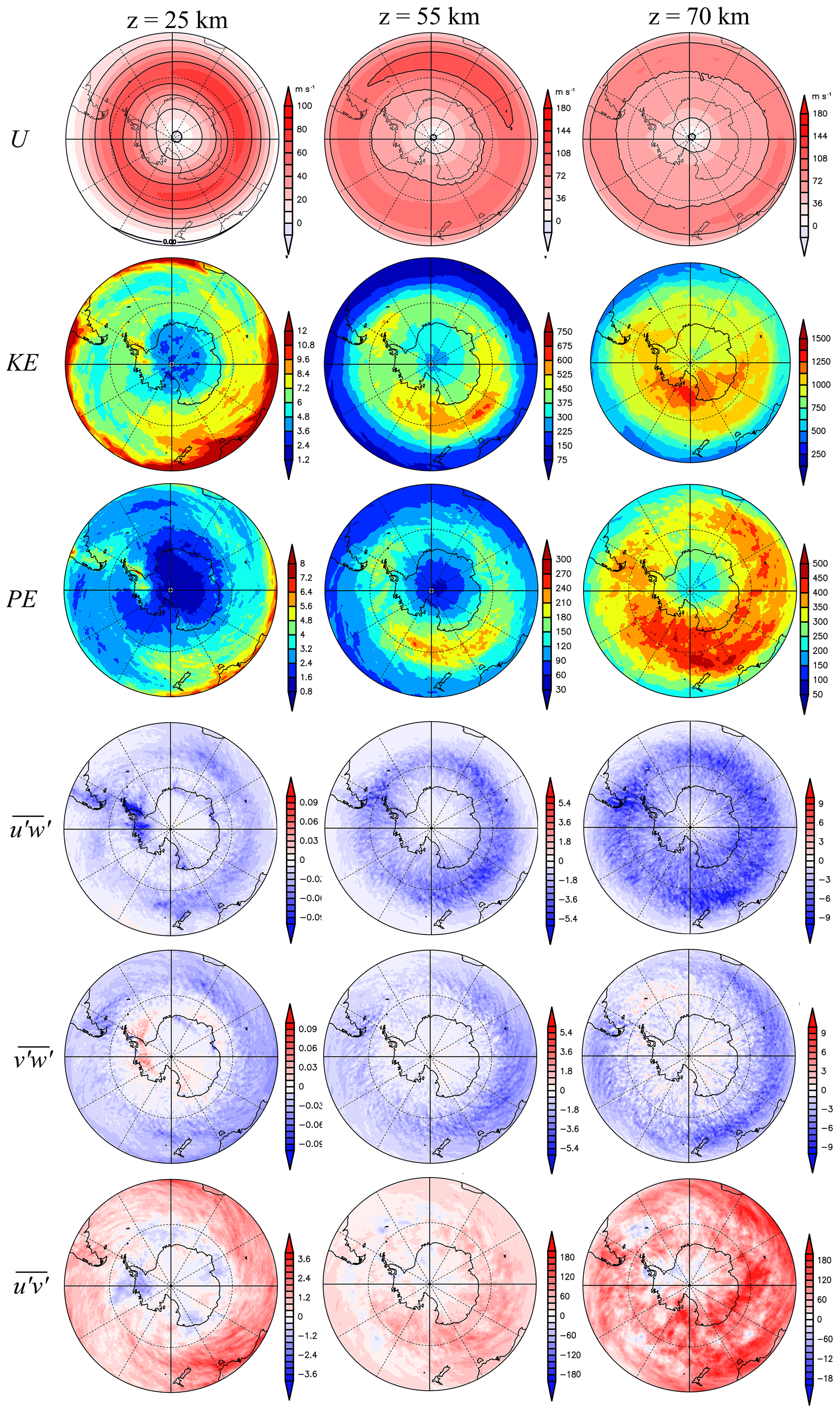
https://www.atmos-chem-phys.net/19/3395/2019/acp-19-3395-2019-f07

Figure 7Horizontal maps of U, $\overline{KE}$ , $\overline{PE}$ , $\overline{u^{'} w^{'}}$ , $\overline{v^{'} w^{'}}$ , and $\overline{u^{'} v^{'}}$ at heights of 25, 55, and 70 km averaged in JJA. The units of U, $\overline{KE}$ , and $\overline{PE}$ and $\overline{u^{'} w^{'}}$ , $\overline{v^{'} w^{'}}$ , and $\overline{u^{'} v^{'}}$ are meters per second, joules per kilogram, and m² s⁻², respectively.

Download

Figure 7 shows horizontal maps of the zonal wind (U), the kinetic energy ( $\overline{KE} = \frac{1}{2} (\overline{u^{' 2}} + \overline{v^{' 2}} + \overline{w^{' 2}})$ ), and the potential energy ( $\overline{PE} = \frac{1}{2} \frac{g^{2}}{N^{2}} \overline{{(\frac{θ^{'}}{\overline{θ}})}^{2}}$ ) divided by the density, $\overline{u^{'} w^{'}}$ , $\overline{v^{'} w^{'}}$ , and $\overline{u^{'} v^{'}}$ at heights of 25, 55, and 70 km averaged over JJA. For the estimation of $\overline{PE}$ , the fluctuation of the potential temperature is calculated as

\begin{matrix} (7) & \frac{θ^{'}}{\overline{θ}} = \frac{1}{ρ_{0}} (\frac{p^{'}}{c_{s}^{2}} - ρ^{'}), \end{matrix}

where c_s denotes the speed of sound in the atmosphere. The axis of the polar night jet tilts equatorward with height, as seen in Fig. 6. For $\overline{KE}$ and $\overline{PE}$ at a height of 25 km, large energies are distributed near 30^∘ S and along the jet axis at approximately 60^∘ S. Localized energy peaks are also seen over the Antarctic Peninsula and the southern Andes and their leeward region, which is consistent with the results of the KANTO model (Sato et al., 2012) and superpressure balloon and satellite observations. For $\overline{KE}$ and $\overline{PE}$ at heights of 55 and 70 km, large values are observed along latitudinal circles roughly corresponding to the axis of the polar night jet. Strictly speaking, the large values of $\overline{KE}$ and $\overline{PE}$ at a height of 55 km appear to be distributed slightly poleward of the axis of the polar night jet, while those of $\overline{KE}$ at a height of 70 km are broadly distributed but are primarily poleward of 60^∘ S. It is interesting that the largest energies are seen near 180^∘ E at heights of 55 and 70 km.

At a height of 25 km, $\overline{u^{'} w^{'}}$ is primarily negative and large values are seen over both the Antarctic Peninsula and the southern Andes. Conversely, $\overline{v^{'} w^{'}}$ is primarily positive over the Antarctic Peninsula and negative over the southern Andes. This result suggests the existence of wave-like structures with phases aligned in the northwest–southeast direction over the southern Andes and in the northeast–southwest direction over the Antarctic Peninsula, which is confirmed by previous observational studies (e.g., Alexander and Barnet, 2007; Hertzog et al., 2008) and by numerical models (e.g., Sato et al., 2012; Plougonven et al., 2013). At higher altitudes, negative values of $\overline{u^{'} w^{'}}$ are distributed along the latitudinal circle near 60^∘ S at a height of 55 km and near 50^∘ S at 70 km. Note that the large negative values over the southern Andes and its leeward region are observed even at a height of 70 km. The signs of $\overline{v^{'} w^{'}}$ are primarily negative along and equatorward of the polar night jet axis and positive or weakly negative poleward of the jet axis at 25 km. This may indicate that the gravity waves propagate into the polar night jet as shown in Sato et al. (2009). The sign of $\overline{u^{'} v^{'}}$ is primarily positive at heights of 55 and 70 km, while it is positive equatorward of 60^∘ S and negative poleward of 60^∘ S at 25 km. These features are consistent with the distributions of $\overline{u^{'} w^{'}}$ and $\overline{v^{'} w^{'}}$ since the signs of $\overline{u^{'} w^{'}}$ and $\overline{v^{'} w^{'}}$ are both negative (Eq. 5). Therefore, it is suggested that the statistical characteristics of disturbances defined as components with wave frequencies higher than 2π∕30 h follow linear relationships of the inertia–gravity waves.

4.2 Spectral analysis

4.2.1 The meridional structure of the power spectra

To examine the statistical characteristics of the mesospheric disturbances simulated by NICAM, the ω power spectra of u, v, w, and the temperature (P_u(ω), P_v(ω), P_w(ω), and P_t(ω), respectively) were obtained for the period of JJA 2016. The power spectra were examined using the Blackman and Tukey (1958) method (e.g., Sato, 1990). First, an autocorrelation function was calculated for each 5-day simulation to avoid any influences of the gaps between the segments of the simulations. Second, to reduce statistical noise in the power spectra estimation, the autocorrelation functions were averaged over JJA. The maximum lag in the calculation of the autocorrelation function was set to 90 h to increase the frequency resolution of the ω spectra; this is 75 % of the simulation period (120 h) in each segment.

Figure 8 shows P_u(ω), P_v(ω), P_w(ω), and P_t(ω) for JJA averaged over heights of 70–75 km at a grid point near Syowa Station. It is seen that P_u(ω) and P_v(ω) have isolated peaks at a frequency of 2π∕12 h, while they obey a power law with an exponent of approximately $- 5 / 3$ for frequencies higher than 2π∕12 h. Such a power-law structure in the high-frequency region is consistent with previous observational studies by MST radars at midlatitudes (e.g., Muraoka et al., 1990) and in the Antarctic (Sato et al., 2017). Conversely, P_w(ω) has a flat structure (i.e., ∝ω⁰) for frequencies from 2π∕2 h to 2π∕5 days and has no clear spectral peak. Finally, P_t(ω) does not have a clear peak at the frequency of 2π∕12 h but rather a broad peak at frequencies near 2π∕10 h. The spectral slope of P_t(ω) is gentler than $- 5 / 3$ but steeper than −1 in the high-frequency region. Here, the flat spectrum of P_w(ω) can be explained by the linear theory of gravity waves. The vertical velocity is proportional to a buoyancy and temperature:

\begin{matrix} (8) & w^{'} = \frac{\hat{ω}}{N^{2}} b^{'}, \end{matrix}

where b^′ denotes a buoyancy by gravity waves. Consequently, the variance of w^′ is proportional to ${\hat{ω}}^{2} b^{' 2}$ . Given a buoyancy and temperature spectrum with a frequency exponent between −1 and $- 5 / 3$ , an exponent for the vertical frequency spectrum becomes nearly zero, which is consistent with the result in Fig. 8.

https://www.atmos-chem-phys.net/19/3395/2019/acp-19-3395-2019-f08

Figure 8Frequency power spectra of (a) zonal, (b) meridional, and (c) vertical wind and (d) temperature fluctuations averaged for the height region of 70–75 km for JJA in NICAM at a grid point near Syowa Station. Vertical black dotted lines indicate frequencies corresponding to 1 day and half a day. Red dotted lines indicate the inertia frequency at Syowa Station ( $\sim 2 π / 12.7$ h at 69^∘ S). Error bars show intervals of the 90 % statistical significance.

Download

Next, the zonally averaged v power spectra (P_v(ω)) in JJA without the diurnal and semidiurnal migrating tides and the semidiurnal non-migrating tides with s=1 were calculated to examine the nontidal low-frequency disturbances (Sato et al., 2017), where s denotes a zonal wavenumber of tides. Hereafter, P_v(ω) without these tides is denoted $\tilde{P_{v}} (ω)$ . The zonal mean $\tilde{P_{v}} (ω)$ in JJA is shown as a function of the latitude for the heights of 70, 55, 40, and 25 km in Fig. 9a, b, c, and d, respectively. The temperature power spectra ( ${\tilde{P}}_{t} (ω)$ ) at a height of 70 km are also shown in Fig. 9e. The thick red dashed curves indicate the inertial frequencies at each latitude. Note that the x axis is the ground-based frequency and not the intrinsic frequency.

https://www.atmos-chem-phys.net/19/3395/2019/acp-19-3395-2019-f09

Figure 9Zonal mean ground-based frequency power spectra of meridional wind fluctuations without diurnal and semidiurnal migrating tides and semidiurnal non-migrating tides with s=1 ( $\tilde{P_{v}} (ω)$ ) averaged in JJA as a function of latitude at heights of (a) 25 km, (b) 40 km, (c) 55 km, and (d) 70 km. (e) Frequency spectra of temperature fluctuations averaged in June and July with horizontal wavelengths longer than 1000 km without the migrating tides at 70 km. Vertical black dotted lines indicate frequencies corresponding to the 1-day period and half day. A red thick dashed curve indicates the inertial frequencies at each latitude.

Download

At a height of 70 km, the spectral peaks appear at frequencies slightly lower than the inertial frequencies from 65 to 75^∘ S, as in Fig. 9a. In the midlatitudes, the spectral values are maximized near 2π∕24 h. Conversely, in regions from 77 to 90^∘ S, the spectral peaks are seen near frequencies from 2π∕8 to 2π∕10 h but are absent at 2π∕12 h (and at the inertial frequencies) or 2π∕24 h. Such peaks near frequencies from 2π∕8 to 2π∕10 h in the high-latitude region also appear in ${\tilde{P}}_{t} (ω)$ (Fig. 9e). In addition, another branch with frequencies smaller than 2π∕50 h, which is an order of a frequency of planetary waves, is found from the midlatitudes to the south pole.

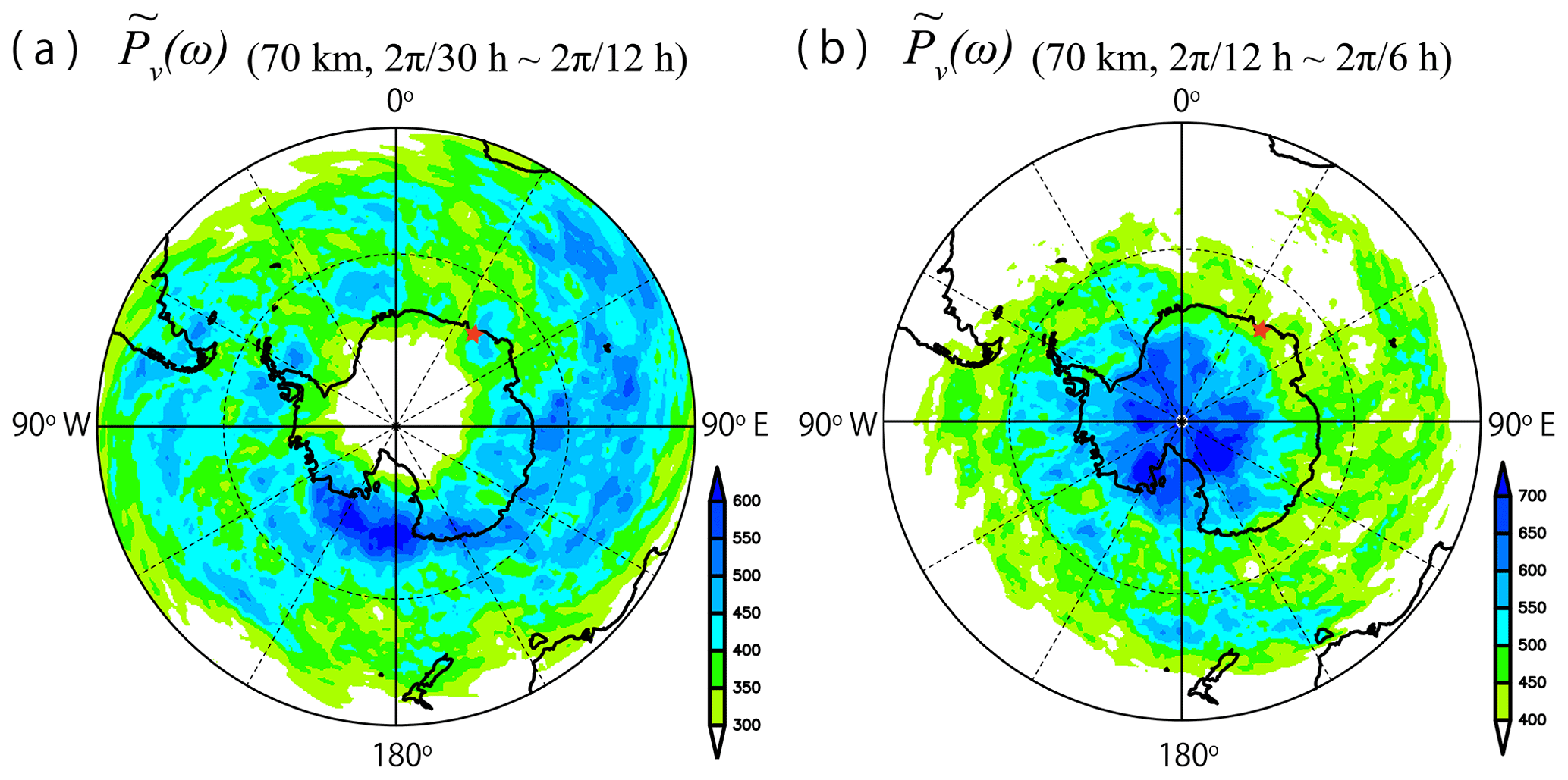
https://www.atmos-chem-phys.net/19/3395/2019/acp-19-3395-2019-f10

Figure 10The horizontal map of $\tilde{P_{v}} (ω)$ contributed by disturbances (a) at the frequencies from (2π∕30 h) to (2π∕12 h) and (b) at the frequencies from (2π∕12 h) to (2π∕6 h) at a height of 70 km. A red star denotes the location of Syowa Station.

Download

The spectral peaks near the inertia frequency are also found in the high-latitude region at a height of 55 km (Fig. 9b). In addition, large spectral values are distributed in the frequency range from the inertial frequencies to 2π∕24 h from 50 to 60^∘ S but not from 30 to 40^∘ S. The spectral peaks near the inertia frequency in the high-latitude region are barely seen at heights of 40 and 25 km, suggesting that such spectral peaks in the high-latitude region are only found in the mesosphere. At a height of 25 km, the spectral values are greatest in the inertial frequencies at midlatitudes from 30 to 40^∘ S, which is consistent with the result shown by Sato et al. (1999) using a high-resolution GCM. Note that energy peaks at frequencies from 2π∕10 to 2π∕8 h in regions from 77 to 90^∘ S are seen at all heights.

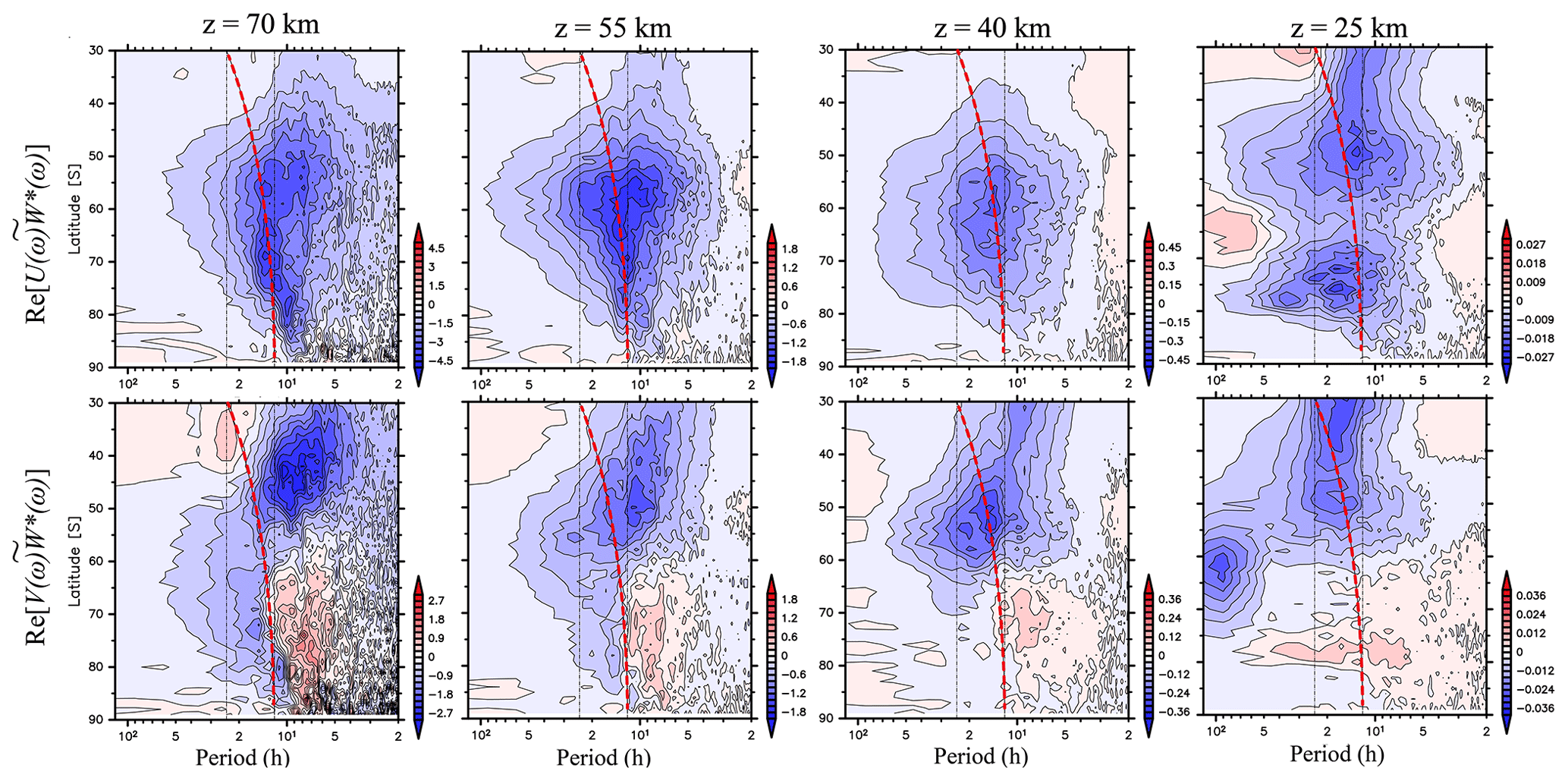
https://www.atmos-chem-phys.net/19/3395/2019/acp-19-3395-2019-f11

Figure 11Zonal mean ground-based frequency power spectra of vertical fluxes of zonal and meridional momentum (Re[U(ω)W^∗(ω)], Re[V(ω)W^∗(ω)]) without diurnal and semidiurnal migrating tides, and semidiurnal non-migrating tides with s=1 averaged in JJA as a function of latitude at heights of 25, 40, 55, and 70 km. Vertical black dotted lines indicate frequencies corresponding to the 1-day period and half day. A red thick dashed curve indicates the inertial frequencies at each latitude.

Download

Here, we focus on the spectral peaks found in Fig. 9a near the inertial frequency from 65 to 75^∘ S and at frequencies from 2π∕10 to 2π∕8 h from 77 to 90^∘ S. The horizontal map of the integration of $\tilde{P_{v}} (ω)$ (i.e., the variance) for frequencies from 2π∕30 to 2π∕12 h at a height of 70 km is shown in Fig. 10a, while that at frequencies from 2π∕12 to 2π∕6 h is shown in Fig. 10b. It appears that variances for frequencies from 2π∕30 to 2π∕12 h are broadly distributed around 180^∘ E at latitudes poleward of 60^∘ S, which is consistent with the distribution of $\overline{KE}$ in Fig. 7. In this frequency range, the energies of the gravity waves are very low near the center of Antarctica. Conversely, the variances for frequencies from 2π∕12 to 2π∕6 h are large over Antarctica and on the ice sheet in the Ross Sea. These features suggest that the dynamical characteristics of the gravity waves, such as the propagation paths, and/or the generation mechanisms may be different in the two frequency ranges.

4.2.2 The meridional structure of the momentum flux spectra

Next, the frequency spectra of vertical fluxes of the zonal and meridional momentum (Re[U(ω)W^∗(ω)], Re[V(ω)W^∗(ω)]) were obtained via the Blackman–Tukey (1958) method. In Fig. 11, zonally averaged Re[U(ω)W^∗(ω)] and Re[V(ω)W^∗(ω)] without diurnal and semidiurnal migrating tides and semidiurnal non-migrating tides with s=1 are shown at heights of 70, 55, 40, and 25 km in JJA. Hereafter, these components are denoted as $Re [\tilde{U (ω) W^{*} (ω)}]$ and $Re [\tilde{V (ω) W^{*} (ω)}]$ , respectively. Note that the contributions of the tides to Re[U(ω)W^∗(ω)] and Re[V(ω)W^∗(ω)] are not large in the mesosphere during the time period of JJA 2016 (not shown).

For $Re [\tilde{U (ω) W^{*} (ω)}]$ , an isolated peak is observed near the inertial frequency from 55 to 75^∘ S at a height of 70 km. Another spectral peak at frequencies from 2π∕10 to 2π∕8 h from 77 to 90^∘ S appears to be similar to that of $\tilde{P_{v}} (ω)$ (Fig. 9). In addition, large spectral values are distributed near 55^∘ S at frequencies from 2π∕12 to 2π∕6 h. The signs of $Re [\tilde{U (ω) W^{*} (ω)}]$ are mostly negative over the entire frequency range. At heights of 55 and 40 km, there are large spectral values of $Re [\tilde{U (ω) W^{*} (ω)}]$ from 65 to 75^∘ S because the isolated peaks are distributed around the inertial frequency from 55 to 60^∘ S but not from 65 to 75^∘ S. At a height of 25 km, two separated spectral peaks are found at frequencies from 2π∕24 to 2π∕12 h. One is centered from 45 to 55^∘ S, while the other is centered from 65 to 80^∘ S.

Conversely, the sign of $Re [\tilde{V (ω) W^{*} (ω)}]$ at a height of 25 km is negative from 45 to 55^∘ S but positive from 65 to 80^∘ S. Under the assumption of upward propagation, it is likely that gravity waves with large negative $Re [\tilde{U (ω) W^{*} (ω)}]$ at a height of 25 km from 45 to 55^∘ S propagate poleward, while those from 65 to 80^∘ S propagate equatorward. At heights of 40 and 55 km, however, $Re [\tilde{V (ω) W^{*} (ω)}]$ around the spectral peak of $Re [\tilde{U (ω) W^{*} (ω)}]$ at slightly lower frequencies than the inertial frequency is mostly negative. These features suggest that the two spectral peaks at a height of 25 km propagate toward 60^∘ S and then merge into an isolated spectral peak at a height of 40 km. At heights from 40 to 70 km, gravity waves at frequencies lower than the inertial frequencies from 60 to 90^∘ S have negative $Re [\tilde{V (ω) W^{*} (ω)}]$ , while those at frequencies higher than the inertial frequencies have positive $Re [\tilde{V (ω) W^{*} (ω)}]$ . From 30 to 60^∘ S, gravity waves at frequencies higher than the inertial frequencies have negative $Re [\tilde{V (ω) W^{*} (ω)}]$ .

https://www.atmos-chem-phys.net/19/3395/2019/acp-19-3395-2019-f12

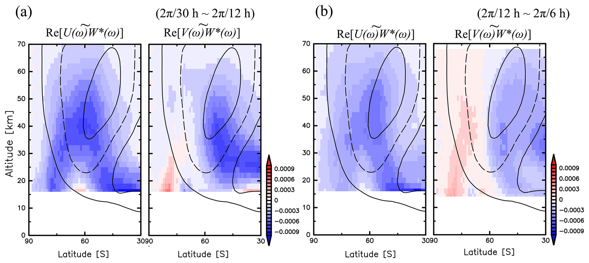
Figure 12Latitudinal structures of an integration of $Re [ρ_{0} \tilde{U (ω) W^{*} (ω)}]$ and $Re [ρ_{0} \tilde{V (ω) W^{*} (ω)}]$ contributed by wave disturbances (a) for the frequencies from (2π∕30 h) to (2π∕12 h) and (b) for the frequencies from (2π∕12 h) to (2π∕6 h) averaged in JJA. The contour values indicate zonal mean zonal wind with a contour interval of 30 m s⁻¹.

Download

To examine these features, the latitude–height sections of $Re [ρ_{0} \tilde{U (ω) W^{*} (ω)}]$ and $Re [ρ_{0} \tilde{V (ω) W^{*} (ω)}]$ for gravity waves at frequencies from 2π∕30 to 2π∕12 h are shown in Fig. 12a, while those from 2π∕12 to 2π∕6 h are shown in Fig. 12b. It is seen that $Re [ρ_{0} \tilde{U (ω) W^{*} (ω)}]$ from both 2π∕30 to 2π∕12 h and 2π∕12 to 2π∕6 h has two branches in the lower stratosphere, which merge southward of the polar night jet axis at a height of approximately 40 km. The signs of $Re [ρ_{0} \tilde{V (ω) W^{*} (ω)}]$ at frequencies from 2π∕30 to 2π∕12 h are positive (negative) at heights below 40 km along the low-latitude (high-latitude) branch of $Re [ρ_{0} \tilde{U (ω) W^{*} (ω)}]$ , while they are primarily negative at heights above 40 km. Conversely, the signs of $Re [ρ_{0} \tilde{V (ω) W^{*} (ω)}]$ at frequencies from 2π∕12 to 2π∕6 h are positive (negative) poleward (equatorward) of 60^∘ S from the lower stratosphere to the mesosphere. These results indicate that gravity waves at frequencies from 2π∕12 to 2π∕6 h propagate into 60^∘ S, which is similar to the previous picture of the meridional propagation of gravity waves discussed by Sato et al. (2009) and Kalisch et al. (2014). However, gravity waves at frequencies from 2π∕30 to 2π∕12 h propagate poleward above a height of 40 km, not into the jet axis. This contrast is inherently related to the existence of the isolated peaks around the inertial frequency at heights of 55–70 km in Fig. 11, which is discussed in detail in Sect. 5. Note that $Re [ρ_{0} \tilde{V (ω) W^{*} (ω)}]$ at frequencies from 2π∕12 to 2π∕6 h has large negative values near a latitude of 30^∘ S at heights above 35 km. This may be related to the meridional propagation of convective gravity waves from the equatorial region, as suggested by an observational study using MF radar (Yasui et al., 2016).

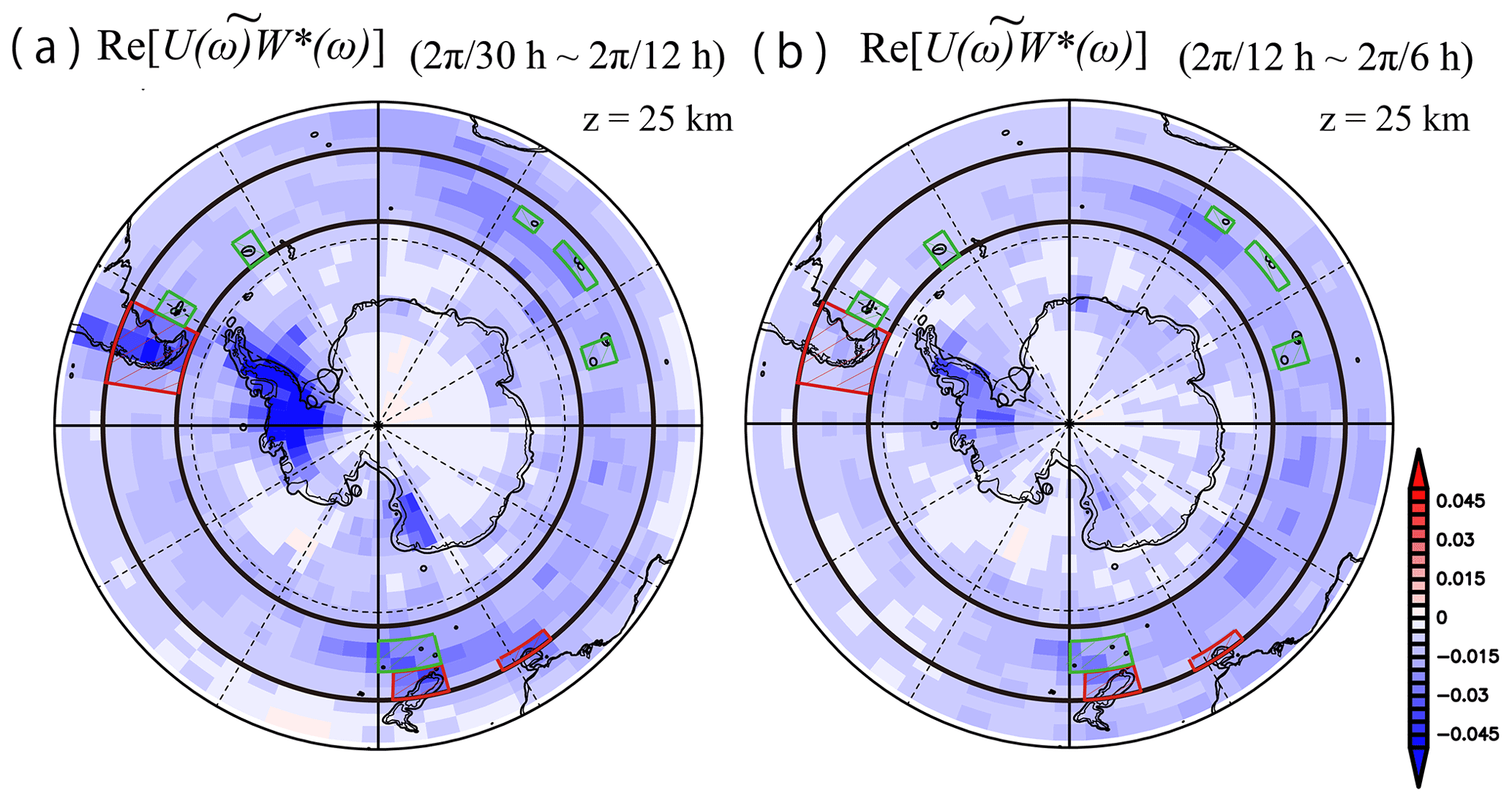
https://www.atmos-chem-phys.net/19/3395/2019/acp-19-3395-2019-f13

Figure 13The horizontal map of $Re [ρ_{0} \tilde{U (ω) W^{*} (ω)}]$ contributed by disturbances (a) at the frequencies from (2π∕30 h) to (2π∕12 h) and (b) at the frequencies from (2π∕12 h) to (2π∕6 h). Regions surrounded by red rectangles and green rectangles denote the domain dominated by the topography and the island, respectively.

Download

A horizontal map of $Re [\tilde{U (ω) W^{*} (ω)}]$ at frequencies from 2π∕30 to 2π∕12 h at a height of 25 km is shown in Fig. 13a, while that at frequencies from 2π∕12 to 2π∕6 h is shown in Fig. 13b. At latitudes from 65 to 80^∘ S, $Re [\tilde{U (ω) W^{*} (ω)}]$ has very large negative values above the Antarctic Peninsula in both Fig. 13a and b. Negative values of $Re [\tilde{U (ω) W^{*} (ω)}]$ are also found along the coast of Antarctica, in particular, above the western side of the Ross Sea. Therefore, it is thought that the poleward branches of $Re [\tilde{U (ω) W^{*} (ω)}]$ shown in Fig. 12 are primarily due to orographic gravity waves. However, note that the gravity waves observed over the coast of Antarctica may be partly due to non-orographic gravity waves caused by spontaneous radiation from the upper tropospheric jet stream (Shibuya et al., 2016).

To examine the contribution of orographic and non-orographic gravity waves to the equatorward branches in Fig. 12, the magnitudes of $Re [\tilde{U (ω) W^{*} (ω)}]$ from 42 to 57^∘ S (the thick black circles in Fig. 13) were estimated over various topographies (the red rectangles), islands (the green rectangles), and the Southern Ocean. The decomposition of these domains is also described in Fig. 13. Over the latitudinal band from 42 to 57^∘ S, the contributions of $Re [\tilde{U (ω) W^{*} (ω)}]$ due to gravity waves at frequencies from 2π∕30 to 2π∕12 h over the topographies, islands, and Southern Ocean are 12.3 %, 6.6 %, and 81.1 %, respectively, while those at frequencies from 2π∕12 to 2π∕6 h are 7.1 %, 6.0 %, and 86.9 %, respectively. Therefore, the equatorward branch of $Re [\tilde{U (ω) W^{*} (ω)}]$ is likely primarily composed of non-orographic gravity waves.

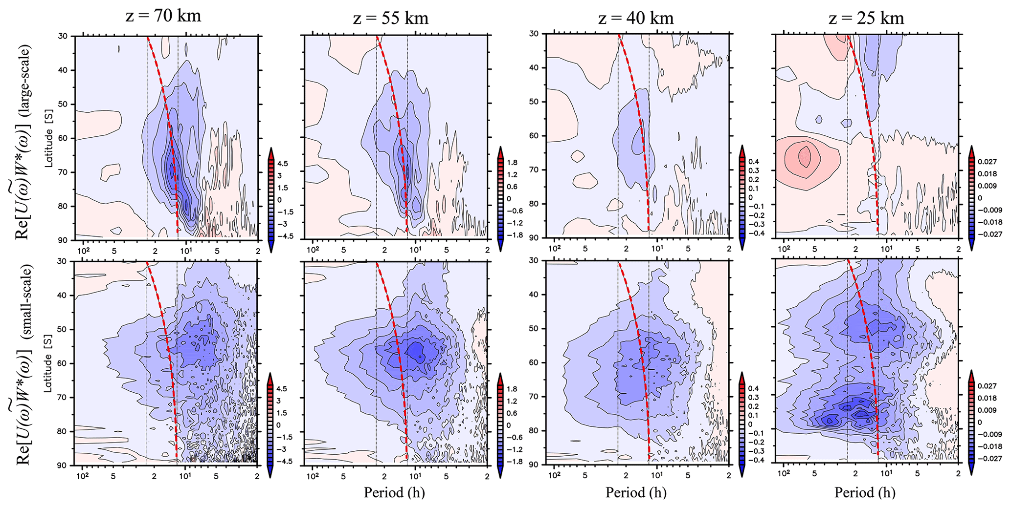
https://www.atmos-chem-phys.net/19/3395/2019/acp-19-3395-2019-f14

Figure 14Zonal mean ground-based frequency power spectra of vertical fluxes of zonal momentum (Re[U(ω)W^∗(ω)]) without diurnal and semidiurnal migrating tides and semidiurnal non-migrating tides with s=1 averaged in JJA as a function of latitude at heights of 25, 40, 55, and 70 km. The upper (lower) line shows Re[U(ω)W^∗(ω)] contributed by disturbances with horizontal scales larger (smaller) than 1000 km. A red thick dashed curve indicates the inertial frequencies at each latitude.

Download

Finally, the horizontal scales of the wave disturbances contributing to $Re [\tilde{U (ω) W^{*} (ω)}]$ were examined at each height. Hereafter, small- to medium-scale (large-scale) wave disturbances are defined as components with horizontal wavelengths smaller than (larger than) 1000 km, as occasionally defined in previous studies (e.g., Geller et al., 2013). To extract the small- to medium-scale and large-scale components, a spatial filter was applied to the wind data gridded in an x–y coordinate system centered at the South Pole as projected by the Lambert azimuthal equal-area projection. Figure 14 shows the zonally averaged $Re [\tilde{U (ω) W^{*} (ω)}]$ resulting from large-scale and small- to medium-scale components during JJA at heights of 70, 55, 40, and 25 km. At heights of 25 and 40 km, it appears that the majority of $Re [\tilde{U (ω) W^{*} (ω)}]$ is composed of small- to medium-scale components, while at heights of 55 and 70 km, the large-scale components have large negative values near the inertial frequencies. This feature is consistent with Shibuya et al. (2017), who showed that mesospheric disturbances with a large amplitude observed at Syowa Station are due to quasi-12 h gravity waves with horizontal wavelengths larger than 1500 km. In addition, it appears that the spectral peak at frequencies from 2π∕8 to 2π∕10 h for the latitude range from 77 to 90^∘ S is also due to large-scale wave disturbances.

5 Discussion

Recently, Sato et al. (2017) estimated the power spectra of horizontal and vertical wind fluctuations and momentum flux spectra over a wide frequency range from 2π∕8 min to 2π∕20 days using continuous PMSE observation data from the PANSY radar over three summer seasons. It was shown that the spectral slope of P_w(ω) at frequencies from 2π∕2 h to 2π∕5 days is nearly flat in the height range of 84–88 km, which is particularly clear in the spectra of observations by the full PANSY system in the 2015–2016 austral summer season. Even though the altitude range and season examined by Sato et al. (2017) are different from those studied in this study, P_w(ω) simulated by NICAM, as shown in Fig. 8c, is consistent with the PANSY radar observations. Moreover, Sato et al. (2017) demonstrated that the power spectrum of the vertical flux of the zonal momentum (Re[U(ω)W^∗(ω)]) has a positive isolated peak near the inertial frequency in the eastward background zonal wind in the summer season. The shape of Re[U(ω)W^∗(ω)] shown in NICAM is consistent with the results of Sato et al. (2017), even though the sign shown in this study is negative under the westward background zonal wind in winter. Conversely, using the Fe Boltzmann lidar at McMurdo Station (166.7^∘ E, 77.8^∘ S), Chen et al. (2016) showed that P_t(ω) has a broad spectrum peak at frequencies from 2π∕3 to 2π∕10 h centered at approximately 2π∕8 h at a height of 85 km in June for the 5 years of 2011–2015, which is also consistent with the P_t(ω) result in Fig. 8d. The latitude–height section of $Re [ρ_{0} \tilde{V (ω) W^{*} (ω)}]$ in Fig. 12b indicates that the spectral peak from 2π∕3 to 2π∕10 h is composed of gravity waves originating over the Antarctic continent. These results indicate that the spectra of the mesospheric disturbances simulated in NICAM are very realistic at high latitudes in the Southern Hemisphere.

The spectral peaks of P_v(ω) without the migrating tides in the mesosphere are simulated near the inertial frequencies at latitudes from 30 to 75^∘ S. Therefore, the quasi-12 h inertia–gravity waves at Syowa Station examined by Shibuya et al. (2017) can be interpreted as quasi-inertial period gravity waves. Moreover, it is shown that Re[U(ω)W^∗(ω)] also has negative isolated peaks near the inertial frequency. One explanation for the existence of these isolated peaks can be derived from the propagation characteristic of the gravity waves following Sato et al. (1999). The horizontal group velocity C_gh and the vertical group velocity C_gz of the gravity waves are expressed as

\begin{matrix} (9) & C_{gh} = \frac{2 m^{2} ({\hat{ω}}^{2} - f^{2})}{k (k^{2} + m^{2})} \frac{k}{|k|} + U \end{matrix}

and

\begin{matrix} (10) & C_{gz} = - \frac{2 m ({\hat{ω}}^{2} - f^{2})}{(k^{2} + m^{2})} . \end{matrix}

It is easily confirmed from Eqs. (9) and (10) that C_gh and C_gz become zero when the intrinsic frequency $\hat{ω}$ is equal to the inertial frequency f at a latitude called the critical latitude. When gravity waves propagate poleward and then reach the critical latitude, the energies of the gravity waves may be accumulated with small C_gh and C_gz and be seen as isolated peaks near the inertial frequency. Therefore, it is likely that the existence of the clear isolated peaks near the inertial frequencies in the mesosphere is explained by the poleward propagation of gravity waves with quasi-inertial frequencies and negative Re[U(ω)W^∗(ω)].

The feature at which the horizontal scales of the gravity waves become larger near the inertial frequency in Fig. 14 is also explained by the accumulation of gravity waves. Assuming that the explicit dependence of the absolute frequency function Ω on x and t is contained entirely in the background wind U(xt) and that the background vertical wind velocity is negligible (Bühler and McIntyre, 2005), the time evolution of the horizontal wavenumber vector is described by

\begin{matrix} (11) & \frac{d_{g}}{d t} (\begin{array}{c} k \\ l \end{array}) = - (\begin{array}{cc} U_{x} & V_{x} \\ U_{y} & V_{y} \end{array}) (\begin{array}{c} k \\ l \end{array}), \end{matrix}

where U denotes the background wind velocity, Ω is defined as $Ω = \hat{ω} + k \cdot U$ , and d_g∕dt denotes the time derivative along the ray defined as $\partial / \partial t + C_{g} \cdot \nabla$ .

Here, the time evolution of the wavenumber is simplified by only considering the meridional shear of the zonal background wind U_y:

\begin{matrix} (12) & \frac{d_{g}}{d t} l = - U_{y} l . \end{matrix}

Because the signs of Re[V(ω)W^∗(ω)] for gravity waves with $\hat{ω} \sim f$ are primarily negative, the signs of l are also negative assuming upward propagation. In the high-latitude region where U_y>0 (Fig. 12), the absolute value of negative l becomes small, indicating an increase in the horizontal wavelengths. Such a deformation is effective for gravity waves with $\hat{ω} \sim f$ due to their small C_gh and C_gz. This is likely the reason why large-scale gravity waves contribute to the spectral peaks of Re[U(ω)W^∗(ω)] near the inertial frequencies primarily in the mesosphere. In addition, the deformation may also contribute to small $Re [\tilde{V (ω) W^{*} (ω)}]$ around f in the mesosphere (Fig. 11) owing to small negative l.

Note again that the analysis in this study is based on the ground-based frequency and not on the intrinsic frequency; the effects of the Doppler shift are inevitably included. Here, the qualitative comprehension of the Doppler shift has been posed in the austral winter mesosphere. In Fig. 12, it was shown that Re[U(ω)W^∗(ω)] has negative spectral values at heights from 25 to 70 km in the high-latitude Southern Hemisphere. This indicates that gravity waves have negative zonal wavenumbers in the westerly jet. As a result, the intrinsic frequency should be larger than the observed frequency (Eq. 3). In addition, gravity waves with relatively low frequencies propagate poleward since the signs of Re[V(ω)W^∗(ω)] at frequencies slightly longer than the inertial frequency are negative (Figs. 11 and 12). In the case with gravity waves propagating poleward with frequencies lower than 2π∕12 h in the Southern Hemisphere, poleward propagation of gravity waves stalls at a latitude where $\hat{ω} \sim f$ . This latitude is poleward of a latitude where “ω” ∼f since $\hat{ω}$ is larger in the high-latitude region. Thus, assuming that the observed frequency of gravity waves is nearly conserved during the propagation, the energy peak likely appears at frequencies slightly smaller than the inertial frequency. In addition, according to the dispersion relation of gravity waves, |k|∕m becomes small at latitudes where $\hat{ω} \sim f$ . As a result, the ratio of the kinetic and potential energies shifts toward the kinetic energies, and then a parcel motion on the gravity waves becomes horizontal. Thus, it is suggested that the isolated peak at frequencies slightly smaller than the inertial frequency is more evident in the spectra of the meridional wind than that of the temperature, which is consistent with the result in Fig. 9.

However, further studies are required to understand the existence of the isolated peaks in the mesosphere. At a height of 25 km, gravity waves with large negative Re[U(ω)W^∗(ω)] tend to prefer frequencies from 2π∕12 to 2π∕24 h, which is related to the existence of the isolated peaks in the mesosphere. The physical reasons why these observed frequencies are preferred are still unclear. Moreover, the signs of Re[V(ω)W(ω)] at the isolated peaks from 2π∕8 to 2π∕10 h from 77 to 90^∘ S are positive throughout the middle atmosphere, suggesting that these peaks are due to gravity waves originating from a region over the Antarctic continent and/or the coastal region and not from low-latitude regions. These points should be examined relative to the generation mechanisms of gravity waves, which are related to the observed frequencies of the gravity waves.

It appears that the quasi-12 h gravity waves have horizontal scales larger than at least 1000 km. Such gravity waves are not fully resolved by the MERRA reanalysis data (Fig. 5), likely because the vertical resolution of MERRA (Δz∼3.2 km) is insufficient to simulate gravity waves with such vertical wavelengths. The momentum deposition caused by the quasi-inertial-period gravity waves may not be calculated by parameterizations because current parameterization schemes focus only on gravity waves with short horizontal wavelengths. The momentum deposition missed from such quasi-inertia–gravity waves may be one of the key components needed to solve the cold-bias problem in the winter–spring polar middle atmosphere.

On the contrary, as mentioned in Sect. 3.2, the high-top NICAM overestimates the wave amplitude in the mesosphere. Lane and Knievel (2005) showed that gravity waves that were vertically propagating in simulations with coarse resolutions become vertically trapped in those with fine resolutions. A similar discussion was also given by Watanabe et al. (2015), although they focused on a vertical resolution in a numerical model. Thus, it is inferred that some simulated gravity waves that propagated to the mesosphere are trapped or breaking in lower altitudes in the actual atmosphere, leading to the overestimation of the wave energy in NICAM compared with the observation.

6 Summary

The first long-term simulation using the high-top non-hydrostatic general circulation model was performed to analyze mesospheric gravity waves in the period from April to August 2016. Successive runs lasting 7 days were run using initial conditions from the MERRA reanalysis data with a 2-day overlap between consecutive runs. The data for the analyses were compiled using the final 5 days of each simulation. The analysis was carefully performed to avoid the influence of artificial gaps between the different runs. Our main results are summarized as follows.

The mesospheric wind fields simulated by NICAM are realistic according to a comparison with the PANSY radar observations, even though the amplitudes of the wind disturbances appear to be larger than those of the observations. In addition, the large-scale structure of the zonally averaged zonal winds in the latitude–height section is also comparable to the features in the MERRA reanalysis data.
Power spectra of the u and v fluctuations at Syowa Station have an isolated peak at the frequency of 2π∕12 h and obey a power law with an exponent of approximately $- 5 / 3$ in the frequency region higher than the inertial frequency f (corresponding to 2π∕12.7 h), while that of w has a flat structure (i.e., ∝ω⁰) at frequencies from 2π∕2 h to 2π∕5 days. The power spectrum of the v fluctuations without the migrating and non-migrating tides has isolated peaks at the ground-based frequencies slightly lower than f at latitudes from 30 to 75^∘ S, while it has isolated peaks at frequencies of approximately 2π∕8 h at latitudes from 78 to 90^∘ S.
The spectrum of the vertical fluxes of the zonal momentum also has isolated peaks at frequencies slightly lower than f at latitudes from 30 to 75^∘ S at a height of 70 km. The isolated peaks are primarily due to gravity waves with horizontal wavelengths of more than 1000 km. The latitude–height structure of the momentum fluxes indicates that the isolated peaks at frequencies slightly lower than f originate from two branches of gravity wave propagation. It is thought that one of the branches, originating from 75^∘ S, is composed of topographic gravity waves generated over the Antarctic Peninsula and its coast, while more than 80 % of the other, originating from 45^∘ S, is composed of non-orographic gravity waves.
It is suggested that the physical explanation for the existence of the isolated peaks in the high-latitude region in the mesosphere is related to the poleward propagation of quasi-inertial frequency gravity waves and the accumulation of wave energies near their inertial frequencies with very small group velocities.

This study offers a quantitative discussion based on high-resolution observations and numerical models. Statistical analyses of inertia–gravity waves in the mesosphere in different seasons are required to understand the momentum budget in the mesosphere combining the PANSY observations and numerical simulations using NICAM.

Data availability

The PANSY radar observation data are available at the project website, http://pansy.eps.s.u-tokyo.ac.jp/en/ (last access: 15 March 2019). Model outputs are available from the corresponding author upon request.

Supplement

The supplement related to this article is available online at: https://doi.org/10.5194/acp-19-3395-2019-supplement.

Author contributions

RS prepared the model data, performed the analysis, and wrote the paper under the supervision of KS. RS and KS contributed to the interpretation and the discussion of the analysis and the results.

Competing interests

The authors declare that they have no conflict of interest.

Acknowledgements

We would like to express ourgratitude to Masaki Satoh, Hisashi Nakamura, Keita Iga, Toshiyuki Hibiya, Makoto Koike, and Hiroaki Miura for their many useful comments and discussions. We also thank Toru Sato at Kyoto University and Takuji Nakamura, Masaki Tsutsumi, Yoshihiro Tomikawa, and Koji Nishimura at the National Institute of Polar Research for their useful comments and discussions. Special thanks are given to colleagues in the atmospheric dynamics laboratory: Masashi Kohma, Arata Amemiya, Soichiro Hirano, Ryosuke Yasui, Yuuki Hayashi, Yuichi Minamihara, Dai Kochin, and Shun Nakajima.

The PANSY multi-institutional project operated by the University of Tokyo and the National Institute of Polar Research (NIPR), and the PANSY radar system was operated by the Japanese Antarctic Research Expedition. All figures shown in this paper were created using the Dennou Club Library (DCL).

This work is supported by FLAGSHIP2020, MEXT with the priority study4 (Advancement of meteorological and global environmental predictions utilizing observational “Big Data”). This study was also supported by the Program for Leading Graduate Schools, MEXT, Japan (RS), partly by the Japan Society for the Promotion of Science (JSPS) Grant-in-Aid Scientific Research (A) 25247075, and partly by JST CREST JPMJCRI663 (KS).

Review statement

This paper was edited by William Ward and reviewed by three anonymous referees.

References

Alexander, M. J. and Barnet, C.: Using satellite observations to constrain parameterizations of gravity wave effects for global models, J. Atmos. Sci., 64, 1652–1665, 2007.

Alexander, M. J. and Teitelbaum, H.: Observation and analysis of a large amplitude mountain wave event over the Antarctic peninsula, J. Geophys. Res.-Atmos., 112, D21103, https://doi.org/10.1029/2006JD008368, 2007.

Alexander, M. J., Geller, M., McLandress, C., Polavarapu, S., Preusse, P., Sassi, F., Sato, K., Eckermann, S., Ern, M., Hertzog, A., Kawatani, Y., Pulido, M., Shaw, T., Sigmond, M., Vincent, R., and Watanabe, S.: Recent developments in gravity wave effects in climate models, and the global distribution of gravity wave momentum flux from observations and models, Q. J. Roy. Meteor. Soc., 136, 1103–1124, 2010.

Arnold, K. S. and She, C. Y.: Metal fluorescence lidar (light detection and ranging) and the middle atmosphere, Contemp. Phys., 44, 35–49, 2003.

Aso, T.: A note on the semidiurnal non-migrating tide at polar latitudes, Earth Planets Space, 59, e21–e24, 2007.

Baumgaertner, A. J. G., McDonald, A. J., Hibbins, R. E., Fritts, D. C., Murphy, D. J., and Vincent, R. A.: Short-period planetary waves in the Antarctic middle atmosphere, J. Atmos. Sol.-Terr. Phy., 70, 1336–1350, https://doi.org/10.1016/j.jastp.2008.04.007, 2008.

Becker, E.: Sensitivity of the upper mesosphere to the Lorenz energy cycle of the troposphere, J. Atmos. Sci., 66, 647–666, https://doi.org/10.1175/2008JAS2735.1, 2009.

Beres, J. H., Alexander, M. J., and Holton, J. R.: A method of specifying the gravity wave spectrum above convection based on latent heating properties and background wind, J. Atmos. Sci., 61, 324–337, 2004.

Blackman, R. B. and Tukey, J. W.: The Measurement of Power Spectra from the Point of View of Communications Engineering, Dover, New York, USA, 1958.

Bloom, S., Takacs, L., DaSilva, A., and Ledvina, D.: Data assimilation using incremental analysis updates, Mon. Weather Rev., 124, 1256–1271, 1996.

Bühler, O. and McIntyre, M. E.: Wave capture and wave-vortex duality, J. Fluid. Mech., 534, 67–95, 2005.

Cámara, A., Lott, F., and Hertzog, A.: Intermittency in a stochastic parameterization of nonorographic gravity waves, J. Geophys. Res.-Atmos., 119, 11905–11919, https://doi.org/10.1002/2014JD022002, 2014.

Charron, M. and Manzini, E.: Gravity waves from fronts: Parameterization and middle atmosphere response in a general circulation model, J. Atmos. Sci., 59, 923–941, 2002.

Chen, C., Chu, X., McDonald, A. J., Vadas, S. L., Yu, Z., Fong, W., and Lu, X.: Inertia–gravity waves in Antarctica: A case study using simultaneous lidar and radar measurements at McMurdo/Scott Base (77.8^∘ S, 166.7^∘ E), J. Geophys. Res.-Atmos., 118, 2794–2808, 2013.

Chen, C., Chu, X., Zhao, J., Roberts, B. R., Yu, Z., Fong, W., Lu, X., and Smith, J. A.: Lidar observations of persistent gravity waves with periods of 3–10 h in the Antarctic middle and upper atmosphere at McMurdo (77.83^∘ S, 166.67^∘ E), J. Geophys. Res.-Space, 121, 1483–1502, https://doi.org/10.1002/2015JA022127, 2016.

Choi, H.-J. and Chun, H.-Y.: Momentum flux spectrum of convective gravity waves. Part I: An update of a parameterization using mesoscale simulations, J. Atmos. Sci., 68, 739–759, https://doi.org/10.1175/2010JAS3552.1, 2011.

Dowdy, A. J., Vincent, R. A., Tsutsumi, M., Igarashi, K., Murayama, Y., Singer, W., and Murphy, D. J.: Polar mesosphere and lower thermosphere dynamics: 1. Mean wind and gravity wave climatologies, J. Geophys. Res., 112, D17104, https://doi.org/10.1029/2006JD008126, 2007.

Eckermann, S. D. and Preusse, P.: Global measurements of stratospheric mountain waves from space, Science, 286, 1534–1537, 1999.

Ern, M., Trinh, Q. T., Preusse, P., Gille, J. C., Mlynczak, M. G., Russell III, J. M., and Riese, M.: GRACILE: a comprehensive climatology of atmospheric gravity wave parameters based on satellite limb soundings, Earth Syst. Sci. Data, 10, 857–892, https://doi.org/10.5194/essd-10-857-2018, 2018.

Forbes, J. M., Makarov, N. A., and Portnyagin, Y. I.: First results from the meteor radar at south pole: A large 12-hour oscillation with zonal wavenumber one, Geophys. Res. Lett., 22, 3247–3250, 1995.

Fritts, D. C.: Errant inferences of gravity wave momentum and heat fluxes using airglow and lidar instrumentation: Corrections and cautions, J. Geophys. Res.-Atmos., 105, 22355–22360, 2000.

Fritts, D. C. and Alexander, M. J.: Gravity wave dynamics and effects in the middle atmosphere, Rev. Geophys., 41, 1003, https://doi.org/10.1029/2001RG000106, 2003.

Fritts, D. C. and Vincent, R. A.: Mesospheric momentum flux studies at Adelaide, Australia: Observations and a gravity wave–tidal interaction model, J. Atmos. Sci., 44, 605–619, 1987.

Fritts, D. C., Smith, R. B., Taylor, M. J., Doyle, J. D., Eckermann, S. D., Doernbrack, A., Rapp, M., Williams, B. P., Pautet, P. D., Bossert, K., Criddle, N. R., Reynolds, C. A., Reinecke, P. A., Uddstrom, M., Revell, M. J., Turner, R., Kaifler, B., Wagner, J. S., Mixa, T., Kruse, C. G., Nugent, A. D., Watson, C. D., Gisinger, S., Smith, S. M., Lieberman, R. S., Laughman, B., Moore, J. J., Brown, W. O., Haggerty, J. A., Rockwell, A., Stossmeister, G. J., Williams, S. F., Hernandez, G., Murphy, D. J., Klekociuk, A. R., Reid, I. M., and Ma, J.: The Deep Propagating Gravity Wave Experiment (DEEPWAVE): An airborne and ground-based exploration of gravity wave propagation and effects from their sources throughout the lower and middle atmosphere, B. Am. Meteorol. Soc., 97, 425–453, https://doi.org/10.1175/BAMS-D-14-00269.1, 2016.

Garcia, F. J., Kelley, M. C., Makela, J. J., and Huang, C.-S.: Airglow observations of mesoscale low-velocity traveling ionospheric disturbances at midlatitudes, J. Geophys. Res., 105, 18407–18415, https://doi.org/10.1029/1999JA000305, 2000.

Garcia, R. R., Smith, A. K., Kinnison, D. E., de la Camara, A., and Murphy, D. J.: Modification of the gravity wave parameterization in the Whole Atmosphere Community Climate Model: Motivation and results, J. Atmos. Sci., 74, 275–291, https://doi.org/10.1175/JAS-D-16-0104.1, 2017.

Gardner, C. S., Kane, T. J., Senft, D. C., Qian, J., and Papen, G. C.: Simultaneous observations of sporadic E, Na, Fe, and Ca⁺ layers at Urbana, Illinois: Three case studies, J. Geophys. Res., 98, 16865–16873, https://doi.org/10.1029/93JD01477, 1993.

Geller, M. A., Alexander, M., Love, P. T., Bacmeister, J., Ern, M., Hertzog, A., and Zhou, T.: A Comparison between Gravity Wave Momentum Fluxes in Observations and Climate Models, J. Climate, 26, 6383–6405, https://doi.org/10.1175/JCLI-D-12-00545.1, 2013.

Hertzog, A., Boccara, G., Vincent, R. A., Vial, F., and Cocquerez, P.: Estimation of gravity wave momentum flux and phase speeds from quasi-Lagrangian stratospheric balloon flights. Part II: Results from the Vorcore campaign in Antarctica, J. Atmos. Sci., 65, 3056–3070, 2008.

Hibbins, R. E., Espy, P. J., Jarvis, M. J., Riggin, D. M., and Fritts, D. C.: A climatology of tides and gravity wave variance in the MLT above Rothera, Antarctica obtained by MFradar, J. Atmos. Sol.-Terr. Phy., 69, 578–588, 2007.

Hibbins, R. E., Marsh, O. J., McDonald, A. J., and Jarvis, M. J.: A new perspective on the longitudinal variability of the semidiurnal tide, Geophys. Res. Lett., 37, L14804, https://doi.org/10.1029/2010GL044015, 2010.

Hindley, N. P., Wright, C. J., Smith, N. D., and Mitchell, N. J.: The southern stratospheric gravity wave hot spot: individual waves and their momentum fluxes measured by COSMIC GPS-RO, Atmos. Chem. Phys., 15, 7797–7818, https://doi.org/10.5194/acp-15-7797-2015, 2015.

Hoffmann, L., Xue, X., and Alexander, M. J.: A global view of stratospheric gravity wave hotspots located with Atmospheric Infrared Sounder observations, J. Geophys. Res.-Atmos., 118, 416–434, https://doi.org/10.1029/2012JD018658, 2013.

Hoffmann, P., Becker, E., Singer, W., and Placke, M.: Seasonal variation of mesospheric waves at northern middle and high latitudes, J. Atmos. Sol.-Terr. Phy., 72, 1068–1079, https://doi.org/10.1016/j.jastp.2010.07.002, 2010.

Jewtoukoff, V., Hertzog, A., Plougonven, R., de la Cámara, A., and Lott, F.: Comparison of gravity waves in the Southern Hemisphere derived from balloon observations and the ECMWF analyses, J. Atmos. Sci., 72, 3449–2468, https://doi.org/10.1175/JAS-D-14-0324.1, 2015.

Jiang, J. H., Eckermann, S. D., Wu, D. L., Hocke, K., Wang, B., Ma, J., and Zhang, Y.: Seasonal variation of gravity wave sources from satellite observation, Adv. Space Res., 35, 1925–1932, 2005.

K-1 Model Developers: K-1 coupled GCM (MIROC) description, K-1 Tech. Rep., 1, 1–34, Univ. of Tokyo, Tokyo, Japan, 2004.

Kalisch, S., Preusse, P., Ern, M., Eckermann, S. D., and Riese, M.: Differences in gravity wave drag between realistic oblique and assumed vertical propagation, J. Geophys. Res.-Atmos., 119, 10081–10099, 2014.

Kovalam, S. and Vincent, R. A.: Intradiurnal wind variations in the midlatitude and high-latitude mesosphere and lower thermosphere, J. Geophys. Res., 108, 4135, https://doi.org/10.1029/2002JD002500, 2003.

Lane, T. P. and Knievel, J. C.: Some effects of model resolution on simulated gravity waves generated by deep, mesoscale convection, J. Atmos. Sci., 62, 3408–3419, 2005.

Liu, H. L., McInerney, J. M., Santos, S., Lauritzen, P. H., Taylor, M. A., and Pedatella, N. M.: Gravity waves simulated by high-resolution Whole Atmosphere Community Climate Model, Geophys. Res. Lett., 41, 9106–9112, 2014.

Louis, J. F.: A parametric model of vertical eddy fluxes in the atmosphere, Bound.-Lay. Meteorol., 17, 187–202, 1979.

Matsuda, T. S., Nakamura, T., Ejiri, M. K., Tsutsumi, M., and Shiokawa, K.: New statistical analysis of the horizontal phase velocity distribution of gravity waves observed by airglow imaging, J. Geophys. Res.-Atmos., 119, 9707–9718, https://doi.org/10.1002/2014JD021543, 2014.

McFarlane, N. A.: The effect of orographically excited gravity wave drag on the general circulation of the lower stratosphere and troposphere, J. Atmos. Sci., 44, 1775–1800, 1987.

McLandress, C., Shepherd, T. G., Polavarau, S., and Beagley, S. R.: Is Missing Orographic Gravity Wave Drag near 60^∘ S the Cause of the Stratospheric Zonal Wind Biases in Chemistry–Climate Models?, J. Atmos. Sci., 69, 802–818, 2012.

Muraoka, Y., Fukao, S., Sugiyama, T., Yamamoto, M., Nakamura, T., Tsuda, T., and Kato, S.: Frequency-spectra of mesospheric wind fluctuations observed with the MU radar, Geophys. Res. Lett., 17, 1897–1900, https://doi.org/10.1029/Gl017i011p01897, 1990.

Murphy, D. J., Forbes, J. M., Walterscheid, R. L., Hagan, M. E., Avery, S. K., Aso, T., Fraser, G. J., Fritts, D. C., Jarvis, M. J., McDonald, A. J., Riggin, D. M., Tsutsumi, M., and Vincent, R. A.: A climatology of tides in the Antarctic mesosphere and lower thermosphere, J. Geophys. Res., 111, D23104, https://doi.org/10.1029/2005JD006803, 2006.

Murphy, D. J., French, W. J. R., and Vincent, R. A.: Long-Period Planetary Waves in the mesosphere and lower thermosphere above Davis, Antarctica, J. Atmos. Sol.-Terr. Phy., 69, 2118–2138, https://doi.org/10.1016/j.jastp.2007.06.008, 2007.

Murphy, D. J., Aso, T., Fritts, D. C., Hibbins, R. E., McDonald, A. J., Riggin, D. M., Tsutsumi, M., and Vincent, R. A.: Source regions for Antarctic MLT non-migrating semidiurnal tides, Geophys. Res. Lett., 36, L09805, https://doi.org/10.1029/2008GL037064, 2009.

Nakanishi, M. and Niino, H.: An improved Mellor-Yamada level-3 model: Its numerical stability and application to a regional prediction of advection fog, Bound.-Lay. Meteorol., 119, 397–407, 2006.

Nicolls, M. J., Varney, R. H., Vadas, S. L., Stamus, P. A., Heinselman, C. J., Cosgrove, R. B., and Kelley, M. C.: Influence of an inertia-gravity wave on mesospheric dynamics: A case study with the Poker Flat Incoherent Scatter Radar, J. Geophys. Res., 115, D00N02, https://doi.org/10.1029/2010JD014042, 2010.

Nishiyama, T., Sato, K., Nakamura, T., Tsutsumi, M., Sato, T., Kohma, M., Nishimura, K., Tomikawa, Y., Ejiri, M. K., and Tsuda, T. T.: Height and time characteristics of seasonal and diurnal variations in PMWE based on 1 year observations by the PANSY radar (69.0^∘ S, 39.6^∘ E), Geophys. Res. Lett., 42, 2100–2108, https://doi.org/10.1002/2015GL063349, 2015.

Nozawa, T., Nagashima, T., Ogura, T., Yokohata, T., Okada, N., and Shiogama, H.: Climate change simulations with a coupled ocean-atmosphere GCM called the Model for Interdisciplinary Research on Climate: MIROC, CGER Supercomput. Monogr. Rep., 12, Cent. For Global Environ. Res., Natl. Inst. for Environ. Stud., Tsukuba, Japan, 2007.

Plougonven, R., Hertzog A., and Guez, L.: Gravity waves over Antarctica and the Southern Ocean: consistent momentum fluxes in mesoscale simulations and stratospheric balloon observations, Q. J. Roy. Meteor. Soc., 139, 101–118, 2013.

Preusse, P., Ern, M., Eckermann, S. D., Warner, C. D., Picard, R. H., Knieling, P., Krebsbach, M., Russell III, J. M., Mlynczak, M. G., Mertens, C. J., and Riese, M.: Tropopause to mesopause gravity waves in August: Measurement and modeling, J. Atmos. Sol.-Terr. Phy., 68, 1730–1751, 2006.

Preusse, P., Eckermann, S. D., Ern, M., Oberheide, J., Picard, R. H., Roble, R. G., Riese, M., Russell III, J. M., and Mlynczak, M. G.: Global ray tracing simulations of the SABER gravity wave climatology, J. Geophys. Res., 114, D08126, https://doi.org/10.1029/2008JD011214, 2009.

Rabier, F., Bouchard, A., Brun, E., Doerenbecher, A., Guedj, S., Guidard, V., Karbou, F., Peuch, V.-H., Amraoui, L. E., Puech, D., Genthon, C., Picard, G., Town, M., Hertzog, A., Vial, F., Cocquerez, P., Cohn, S. A., Hock, T., Fox, J., Cole, H., Parsons, D., Powers, J., Romberg, K., Van An del, J., Deshler, T., Mercer, J., Haase, J. S., Avallone, L., Kalnajs, L., Mechoso, C. R., Tangborn, A., Pellegrini, A., Frenot, Y., Thepaut, J.-N., McNally, A. P., Balsamo, G., and Steinle, P.: The Concordiasi project in Antarctica, B. Am. Meteorol. Soc., 91, 69–86, 2010.

Reid, I. M. and Vincent, R. A.: Measurements ofmesospheric gravity wave momentum fluxes and mean flow accelerations at Adelaide, Australia, J. Atmos. Terr. Phys., 49, 443–460, 1987.

Richter, J. H., Sassi, F., and Garcia, R. R.: Toward a physically based gravity wave source parameterization in a general circulation model, J. Atmos. Sci., 67, 136–156, 2010.

Rienecker, M., Suarez, M. J., Gelaro, R., Todling, R., Bacmeister, J., Liu, E., Bosilovich, M. G., Schubert, S. D., Takacs, L., Kim, G.-K., Bloom, S., Chen, J., Collins, D., Conaty, A., da Silva, A., Gu, W., Joiner, J., Koster, R. D., Lucchesi, R., Molod, A., Owens, T., Pawson, S., Pegion, P., Redder, C. R., Reichle, R., Robertson, F. R., Ruddick, A. G., Sienkiewicz, M., and Woollen, J.: MERRA: NASA's ModernEra Retrospective Analysis for Research and Applications, J. Climate, 24, 3648–3624, 2011.

Sakazaki, T., Fujiwara, M., Zhang, X., Hagan, M., and Forbes, J.: Diurnal tides in the troposphere to the lower mesosphere as deduced from TIMED/SABER satellite data and six global reanalysis data sets, J. Geophys. Res., 117, D13108, https://doi.org/10.1029/2011JD017117, 2012.

Sato, K.: Vertical wind disturbances in the troposphere and lower stratosphere observed by the MU radar, J. Atmos. Sci., 47, 2803–2817, 1990.

Sato, K. and Yoshiki, M.: Gravity wave generation around the polar vortex in the stratosphere revealed y 3-houly radiosonde observations at Syowa Station, J. Atmos. Sci., 65, 3719–3735, 2008.

Sato, K., Kumakura, T., and Takahashi, M.: Gravity waves appearing in a high-resolution GCM simulation, J. Atmos. Sci., 56, 1005–1018, 1999.

Sato, K., Watanabe, S., Kawatani, Y., Tomikawa, Y., Miyazaki, K., and Takahashi, M.: On the origins of mesospheric gravity waves, Geophys. Res. Lett., 36, L19801, https://doi.org/10.1029/2009GL039908, 2009.

Sato, K., Tateno S., Watanabe, S., and Kawatani, Y.: Gravity wave characteristics in the Southern Hemisphere revealed by a high-resolution middle-atmosphere general circulation model, J. Atmos. Sci., 69, 1378–1396, https://doi.org/10.1175/JAS-D-11-0101.1, 2012.

Sato, K., Tsutsumi, M., Sato, T., Nakamura, T., Saito, A., Tomikawa, Y., Nishimura, K., Kohma, M., Yamagishi, H., and Yamanouchi, T.: Program of the Antarctic Syowa MST/IS Radar (PANSY), J. Atmos. Sol.-Terr. Phy., 118A, 2–15, 2014.

Sato, K., Kohma, M., Tsutsumi, M., and Sato, T.: Frequency spectra and vertical profiles of wind fluctuations in the summer Antarctic mesosphere revealed by MST radar observations, J. Geophys. Res.-Atmos., 122, 3–19, 2017.

Satoh, M., Matsuno, T., Tomita, H., Miura, H., Nasuno, T., and Iga, S.: Nonhydrostatic icosahedral atmospheric model (NICAM) for global cloud resolving simulations, J. Comput. Phys., 227, 3486–3514, https://doi.org/10.1016/j.jcp.2007.02.006, 2008.

Satoh, M., Tomita, H., Yashiro, H., Miura, H., Kodama, C., Seiki, T., Noda, A. T., Yamada, Y., Goto, D., Sawada, M., Miyoshi, T., Niwa, Y., Hara, M., Ohno, T., Iga, S., Arakawa, T., Inoue, T., and Kubokawa, H.: The Non-hydrostatic Icosahedral Atmospheric Model: Description and Development, Progress in Earth and Planetary Science, 1, 18, https://doi.org/10.1186/s40645-014-0018-1, 2014.

Scinocca, J. F.: An accurate spectral nonorographic gravity wave drag parameterization for general circulation models, J. Atmos. Sci., 60, 667–682, 2003.

Sekiguchi, M. and Nakajima, T.: A k-distribution-based radiation code and its computational optimization for an atmospheric general circulation model, J. Quant. Spectrosc. Ra., 109, 2779–2793, 2008.

Shibuya, R., Sato, K., Tomikawa, Y., Tsutsumi, M., and Sato, T.: A study of multiple tropopause structures caused by inertia-gravity waves in the Antarctica, J. Atmos. Sci., 72, 2109–2130, 2015.

Shibuya R., Miura, H., and Sato, K.: A grid transformation method for a quasi-uniform, circular fine region using the spring dynamic, J. Meteorol. Soc. Jpn., 94, 443–452, https://doi.org/10.2151/jmsj.2016-022, 2016.

Shibuya, R., Sato, K., Tsutsumi, M., Sato, T., Tomikawa, Y., Nishimura, K., and Kohma, M.: Quasi-12 h inertia–gravity waves in the lower mesosphere observed by the PANSY radar at Syowa Station (39.6^∘ E, 69.0^∘ S), Atmos. Chem. Phys., 17, 6455–6476, https://doi.org/10.5194/acp-17-6455-2017, 2017.

Song, I. S. and Chun, H. Y.: Momentum flux spectrum of convectively forced internal gravity waves and its application to gravity wave drag parameterization. Part I: Theory, J. Atmos. Sci., 62, 107–124, 2005.

SPARC: SPARC CCMVal Report on the Evaluation of Chemistry-Climate Models, edited by: Eyring, V., Shepherd, T., and Waugh, D., SPARC Report No. 5, WCRP-30/2010, WMO/TD – No. 40, available at: http://www.sparc-climate.org/publications/sparc-reports/ (last access: 18 March 2019), 2010.

Takata, K., Emori, S., and Watanabe, T.: Development of the minimal advanced treatments of surface interaction and runoff, Global Planet. Change, 38, 209–222, 2003.

Talaat, E. R. and Mayr, H. G.: Model of semidiurnal pseudo tide in the high-latitude upper mesosphere, J. Atmos. Sol.-Terr. Phy., 73, 2386–2391, 2011.

Tomikawa, Y., Sato, K., Watanabe, S., Kawatani, Y., Miyazaki, K., and Takahashi, M.: Growth of planetary waves and the formation of an elevated stratopause after a major stratospheric sudden warming in a T213L256 GCM, J. Geophys. Res., 117, D16101, https://doi.org/10.1029/2011JD017243, 2012.

Tomita, H.: New microphysical schemes with five and six categories by diagnostic generation of cloud ice, J. Meteorol. Soc. Jpn., 86A, 121–142, 2008.

Tomita, H., Satoh, M., and Goto, K.: An optimization of icosahedral grid by using spring dynamics, J. Comp. Phys., 183, 307–331, 2002.

Tsutsumi, M., Tsuda, T., Nakamura, T., and Fukao, S.: Temperature fluctuations near the mesopause inferred from meteor observations with the middle and upper atmosphere radar, Radio Sci., 29, 599–610, https://doi.org/10.1029/93RS03590, 1994.

Watanabe, S. and Miyahara, S.: Quantification of the gravity wave forcing of the migrating diurnal tide in a gravity wave-resolving general circulation model, J. Geophys. Res., 114, D07110, https://doi.org/10.1029/2008JD011218, 2009.

Watanabe, S., Kawatani, Y., Tomikawa, Y., Miyazaki, K., Takahashi, M., and Sato, K.: General Aspects of a T213L256 Middle Atmosphere General Circulation Model, J. Geophys. Res., 113, D12110, https://doi.org/10.1029/2008JD010026, 2008.

Watanabe, S., Sato, K., Kawatani, Y., and Takahashi, M.: Vertical resolution dependence of gravity wave momentum flux simulated by an atmospheric general circulation model, Geosci. Model Dev., 8, 1637–1644, https://doi.org/10.5194/gmd-8-1637-2015, 2015.

Wu, D. L. and Waters, J. W.: Satellite observations of atmospheric variances: A possible indication of gravity waves, Geophys. Res. Lett., 23, 3631–3634, 1996.

Wu, D. L., Preusse, P., Eckermann, S. D., Jiang, J. H., de la Torre Juarez, M., Coy, L., and Wang, D. Y.: Remote sounding of atmospheric gravity waves with satellite limb and nadir techniques, Adv. Space Res., 37, 2269–2277, 2006.

Wu, W.-S., Purser, R. J., and Parrish, D. F.: Three-dimensional variational analysis with spatially inhomogeneous covariances, Mon. Weather Rev., 130, 2905–2916, 2002.

Yamashita, C., England, S. L., Immel, T. J., and Chang, L. C.: Gravity wave variations during elevated stratopause events using SABER observations, J. Geophys. Res.-Atmos., 118, 5287–5303, 2013.

Yasui, R., Sato, K., and Tsutsumi, M.: Seasonal and interannual variation of mesospheric gravity waves based on MF radar observations over 15 years at Syowa Station in the Antarctic, SOLA, 12, 46–50, https://doi.org/10.2151/sola.2016-010, 2016.

Yoshiki, M. and Sato, K.: A statistical study of gravity waves in the polar regions based on operational radiosonde data, J. Geophys. Res., 105, 17995–18011, 2000.

Zülicke, C. and Becker, E.: The structure of the mesosphere during sudden stratospheric warmings in a global circulation model, J. Geophys. Res.-Atmos., 118, 2255–2271, https://doi.org/10.1002/jgrd.50219, 2013.

Articles

Download

Article (12137 KB)
Full-text XML

Short summary

The first long-term simulation using the high-top non-hydrostatic general circulation model (NICAM) was executed to analyze mesospheric gravity waves. A new finding in this paper is that the spectrum of the vertical fluxes of the zonal momentum has an isolated peak at frequencies slightly lower than f at latitudes from 30 to 75° S at a height of 70 km. This study discusses the physical mechanism for an explanation of the existence of the isolated spectrum peak in the mesosphere.