2.1 Activities within the POLSTRACC mission

The polar LMS during the Arctic winter 2015/2016 has been probed within the POLar STRAtosphere in a Changing Climate (POLSTRACC) aircraft campaign, using the German High Altitude and LOng Range Research Aircraft (HALO). The mission objectives comprise studying (i) the structure, composition and dynamics of the Arctic winter LMS, (ii) chemical processes that affect ozone in the Arctic winter upper troposphere–lower stratosphere (UTLS), (iii) PSCs and de-/nitrification, and (iv) cirrus clouds in the Arctic UTLS. In a joint effort for the missions POLSTRACC–Gravity Wave Life Cycle Experiment (GW-LCYCLE II)–Seasonality of Air mass transport and origin in the Lowermost Stratosphere (SALSA) (combined under the acronym “PGS”), HALO performed a total of 18 science flights. The long-range capability has been extensively used during the 156 flight hours. Spreading from the campaign bases in Oberpfaffenhofen (EDMO), Germany, and Kiruna (ESNQ), Sweden, the flight tracks span a region between 25–87^∘ N and 80^∘ W–28^∘ E over Europe, the North Atlantic and Greenland (map in Fig. 1). Potential temperatures at flight level reached a maximum of 411 K. Chronologically, the observations cover most of the evolution of the polar vortex: two flights sampled the early winter formation of the vortex in mid-December; the first major campaign phase in January (eight flights) was dedicated to the established vortex, while the second major phase from the end of February to mid-March (eight flights) witnessed the late stages of vortex evolution including the major final warming (MFW) and vortex split. HALO was equipped with a set of in situ and remote-sensing instruments, measuring atmospheric quantities at, below, above and alongside the aircraft position.

Figure 1Map of flight tracks of the PGS science flights. Red stars mark the two bases of operation Oberpfaffenhofen (EDMO) at 48^∘ N, 11^∘ E and Kiruna (ESNQ) at 68^∘ N, 20^∘ E. Flight sections where polar vortex air was encountered according to the criterion from Sect. 2.4.1 are indicated in blue.

The Arctic polar vortex during the winter 2015/2016 has already been subject to a number of studies, most of them directly related to POLSTRACC activities. Overviews of the evolution of the polar vortex are given by Manney and Lawrence (2016), Matthias et al. (2016) and Khosrawi et al. (2017) including satellite, reanalysis and model perspectives. Concurrently, the authors point out the exceptional strength of the vortex due to reduced planetary wave activity, accompanied by record low temperatures and extensive denitrification, dehydration and chlorine activation. Record ozone loss comparable to the extreme winter 2010/2011 (e.g. Sinnhuber et al., 2011) was only prevented by an early onset of sudden stratospheric warming (SSW) and vortex splitting events. The study by Khosrawi et al. (2017) also points to deficiencies in the representation of downward transport and chlorine chemistry in the chemistry–climate model EMAC that may significantly impact chlorine partitioning in the LMS. The formation of PSCs has been investigated by Voigt et al. (2018) with a focus on the pathways of ice PSC nucleation and Dörnbrack et al. (2017) studied a case of gravity-wave-induced PSC formation. A novel approach of three-dimensional visualization of gravity waves from remote tomographic sampling with the Gimballed Limb Observer for Radiance Imaging of the Atmosphere (GLORIA) has been presented by Krisch et al. (2017), while Johansson et al. (2018) examined how the same instrument consistently fills the gap between high-coverage spaceborne sampling and accurate high-resolution in situ measurements. Krause et al. (2018) used chemical tracers to reveal the influence of mixing at the lower vortex edge on the age spectrum of the air.

2.2 Airborne in situ measurements

This section provides an overview of the measurement principles of the in situ instruments used in the present work. In addition to the dedicated trace gas measurements, the Basis HALO Measurement and Sensor System (BAHAMAS) provides meteorological parameters along the flight trajectory (Krautstrunk and Giez, 2012; Giez et al., 2017).

2.2.4 Instrument comparison

In order to assess the data quality, simultaneously measured quantities from the AIMS and GhOST instruments are compared in unperturbed conditions where the sum of reservoir gases equals the amount of Cl_y. To this end, Fig. 2 displays a comparison of AIMS and GhOST data for flight 04 of the PGS campaign. This was the first science flight carried out on 17 December 2015. It started in Oberpfaffenhofen (EDMO) and was headed to the Atlantic Ocean north of Ireland, up to 59.8^∘ N, in order to horizontally cut the tropopause at high altitude in the north–south direction. Polar vortex air was only sparsely hit because the vortex at this time of the year was higher than the maximum altitude of HALO (Matthias et al., 2016). At this early stage of the vortex development, no activated chlorine is expected and as a consequence, inorganic chlorine is expected to be partitioned entirely into the reservoir species HCl and ClONO₂. The simultaneous measurements of AIMS and GhOST are compared in Fig. 2b. Gaps in the AIMS data occur during in-flight calibration and background measurements. AIMS measurements were averaged to the lower time resolution of GhOST to numerically compare the measurements of both instruments. Figure 2a shows (HCl + ClONO₂) − Cl_y relative to Cl_y as a function of time. For the most part, the data agree within ±20 %, which is well within the measurement uncertainty. Larger deviations are only found in tropospheric sections of the flight, where the correlation of CFC-12 and Cl_y is less robust since it varies with tropospheric sources. As shown in Fig. 2c, the correlation between (HCl + ClONO₂) and Cl_y for this flight is linear over the whole concentration range with R²=0.989. Overall, the agreement is excellent, given that this comparison aggregates three independently measured gases and one derived trace gas. Similarly, but not shown here, ClONO₂ (Johansson et al., 2018) and HNO₃ data (e.g. Ungermann et al., 2015) from AIMS compare well to other in situ measurements and remote-sensing products aboard HALO.

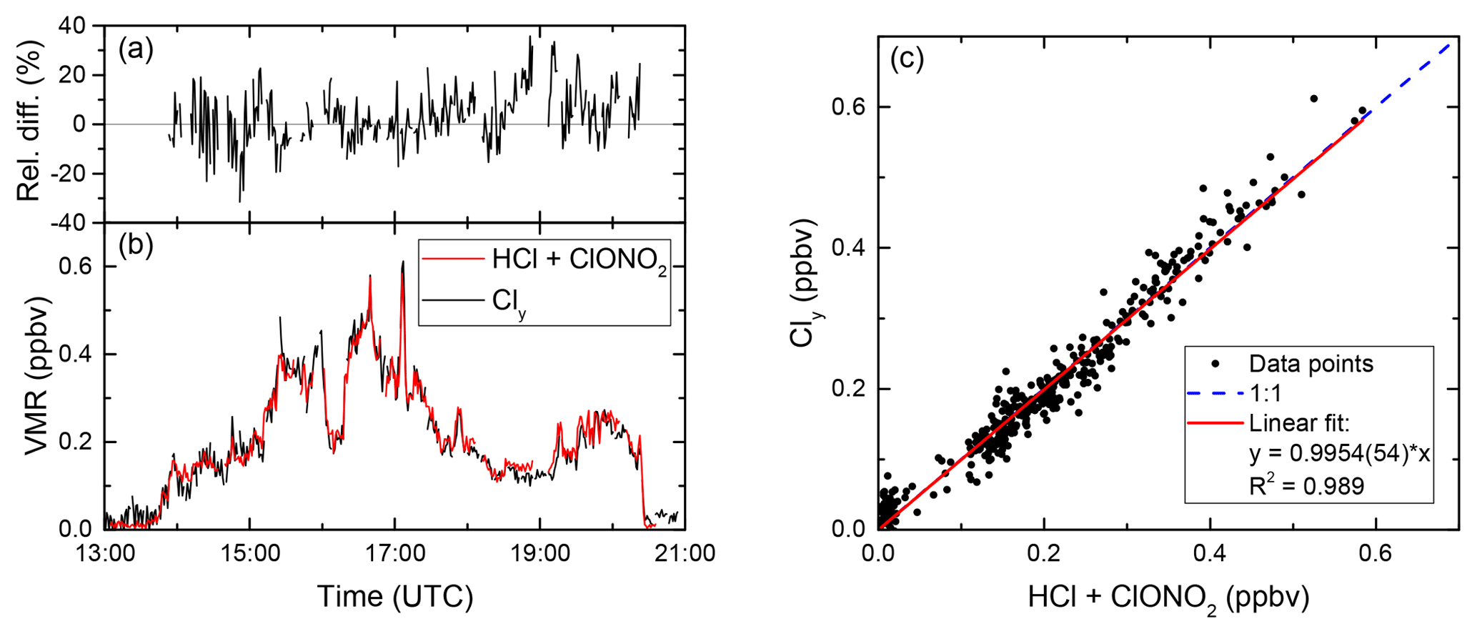
Figure 2Comparison of the sum of HCl and ClONO₂, measured by AIMS, to Cl_y, inferred from GhOST measurements, during flight 04 on 17 December 2015. (a) Difference between both curves relative to Cl_y and (b) timeline of mixing ratios over the whole course of the flight. (c) Correlation between added AIMS measurements and Cl_y.

Download

2.3 Chemical transport model

Simulations are performed with the Chemical Lagrangian Model of the Stratosphere (CLaMS) that is described elsewhere (Grooß et al., 2014, and references therein). Unlike most other Eulerian models, the Lagrangian chemical transport model CLaMS calculates the chemical composition along air parcels irregularly distributed over space that individually follow their trajectories. The underlying wind and temperature data are taken from ECMWF ERA-Interim data (Dee et al., 2011). Initialization and boundary conditions of the model simulation for the winter 2015/2016 are described by Grooß et al. (2018).

Typically, the model output is written every day at 12:00 UTC. For interpolation to the observation locations and times, a Lagrangian mapping was used, employing back trajectories from the desired positions and times to the previous day. The interpolated model output is then taken as the initial state for the CLaMS chemistry module integrated forward to the observation point. With that procedure, the chemical composition (including the simulated chlorine partitioning) at the observation location and time is determined from the model.

2.4 Vortex identification

2.4.1 Identification of vortex air by in situ measurements

The study of chlorine partitioning within this work is intended to focus solely on air masses that can be attributed to the Arctic polar stratospheric vortex. A common means for vortex identification is the Nash criterion (Nash et al., 1996), essentially defining the location of the vortex edge by the maximum gradient of potential vorticity (PV) on isentropic surfaces. In this work, however, the method of Greenblatt et al. (2002) is applied where vortex air is identified by a tight correlation between the inert tracer N₂O and potential temperature. Using this method, the subsequent analysis benefits from the high resolution of measurements of N₂O and potential temperature in contrast to reanalysis PV fields. Thus, small-scale patterns at a size of several kilometres or filamentary structures can be assigned correctly. Figure 3 aggregates all N₂O data points from the PGS campaign versus potential temperature (θ). The plot shows data for potential temperatures above 320 K to focus on the stratosphere above the ExTL at high latitudes. The observed N₂O:θ profile narrows towards the tropopause, whereas it widens towards higher altitudes, showcasing the wide variety of air masses sampled during the flights. The labels in the upper part of Fig. 3 roughly indicate the region of the sampled air masses. Generally three regimes can be distinguished: the vortex regime is found at the inclined left edge of the profile characterized by a strong vertical gradient of N₂O mixing ratio, which connects the tropospheric source region to the photochemical sink in the middle stratosphere (Schmeltekopf et al., 1977). The gradient is maintained by the stratification and isolation of the polar vortex, while isentropic homogeneity leads to a compact form of the profile. At the other extreme, air from mid-latitudes exhibits a more variable gradient in N₂O due to altering influence from tropical or polar air. The lower N₂O mixing ratios inside the vortex, on constant isentropes, result from the large-scale descent of N₂O-poor air from higher altitudes. Both regimes merge towards the troposphere, where the vortex transport barrier vanishes. In between at higher altitudes, we find the boundary region with a continuous shift between vortex and mid-latitude contributions.

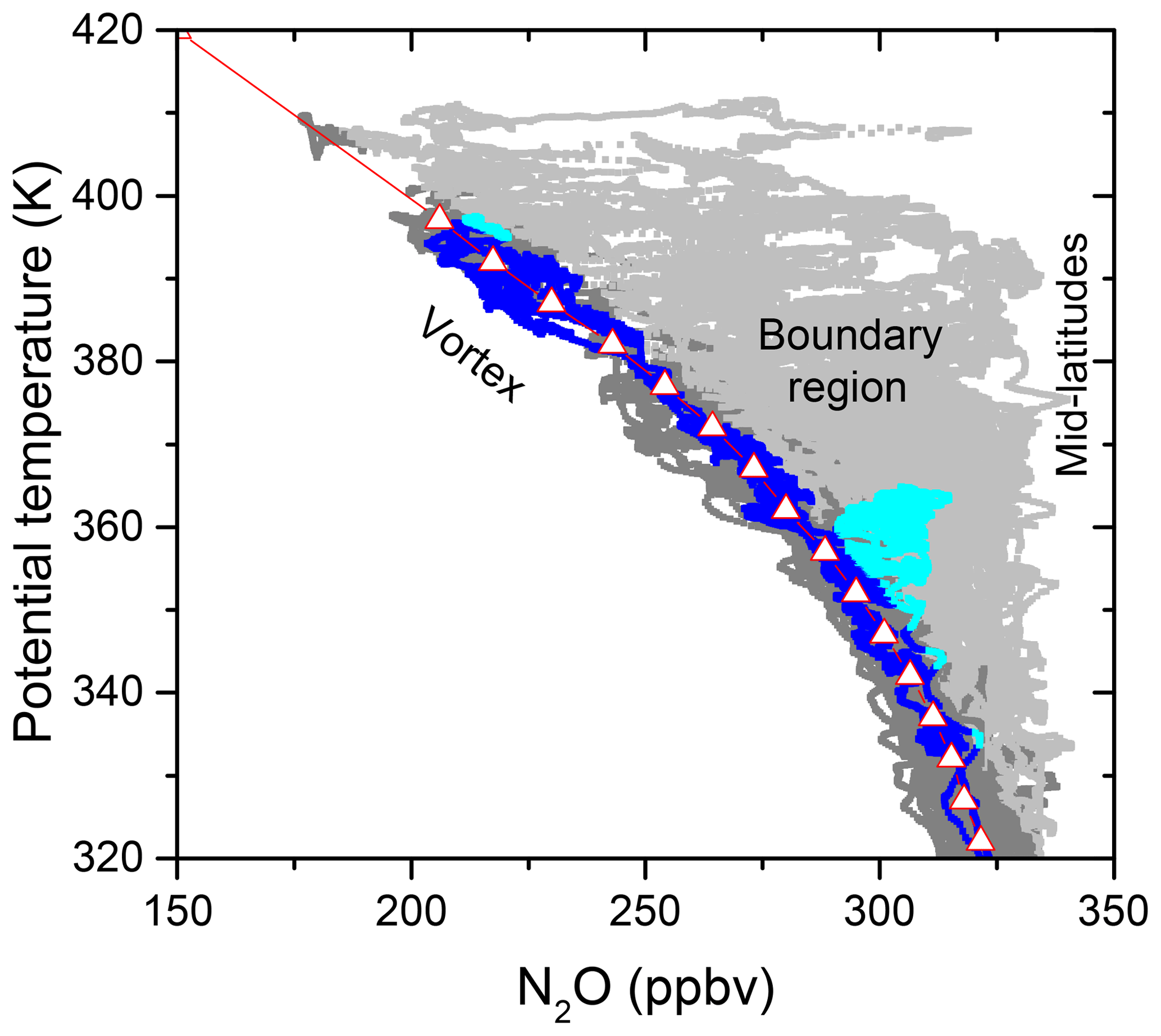
Figure 3Profiles of N₂O versus potential temperature for the whole PGS campaign (grey) and for the selected flight 14, of 26 February 2016 (blue), above 320 K. The derived vortex reference profile is illustrated by the triangles, connected by straight red lines. Dark and light subsets of the grey and blue points indicate the assigned vortex air and extra-vortex air property, respectively.

Download

A flight on 26 February 2016 (flight 14) provides a reference profile, reaching well into the vortex and capturing dynamically unperturbed vortex conditions. The flight exhibits a very compact relationship between N₂O and θ for a wide range of potential temperatures at the lower left edge of the dataset in Fig. 3 (blue points). N₂O measurements from this flight are binned in 5 K intervals of θ, and the mean values are taken as the vortex reference profile (triangles in Fig. 3). Observations also include outside-vortex air as indicated by the light blue points between 345 and 360 K, so the vortex reference points in this range are determined by a quadratic interpolation between the adjoining sections. Beyond 395 K, the vortex reference profile is set by linear extrapolation. A symmetric envelope is placed around the vortex reference profile. The width is determined for each flight individually by the maximum deviation of N₂O data points below the vortex reference value in each bin. All data points lying within the envelope are then considered to belong to vortex air masses (dark points in Fig. 3). This procedure is chosen to sensibly include a high number of measurements in the vortex regime, accounting for instrumental noise and small atmospheric variability while the criterion is not weakened too much. Hereafter, the term “vortex air” is meant to refer to measurements that fulfil the vortex criterion above 320 K. Equally, the term “extra-vortex air” is the complementary set of measurements above 320 K.

Although the determined vortex reference correlation seems to be appropriate for the whole dataset at first glance, we have to account for diabatic descent during the 3-month campaign phase. Satellite data of N₂O (Manney and Lawrence, 2016) and analysis of the in situ N₂O data (Krause et al., 2018) indicate that below θ=450 K, diabatic descent, i.e. descent of air masses versus isentropic surfaces, was strongest before the end of December 2015. Accordingly, the vortex reference profile from flight 14 was lifted by 15 K only for the two December flights, while left unchanged for the rest of the flights.

3.1 Overview of vortex air sampling

The flights of the PGS campaign were conducted from 17 December 2015 until 18 March 2016, covering several stages of evolution of the Arctic polar vortex. The map in Fig. 1 depicts vortex air sampling sections of the conducted flights in blue, as opposed to extra-vortex air sections in black. Two different patterns can be clearly distinguished: On the one hand, there are flights with long sections entirely inside the vortex, resulting in a good sampling statistics and providing insight into intra-vortex variability. On the other hand, many flights exhibit only a patchy sampling of vortex air whenever other objectives of the PGS campaign were pursued. As an example, the PV maps in Fig. 4 illustrate that a compact vortex signature is visible at 50 hPa (above 20 km altitude), whereas it becomes more spread-out and filamented below. On that particular day, vortex air measurements could be conducted over Greenland and northern Canada near the PV maximum on 150 hPa, which is the approximate flight altitude. Split-off parts of vortex air could also be found at latitudes down to 42.7^∘ N towards the end of the campaign in early spring.

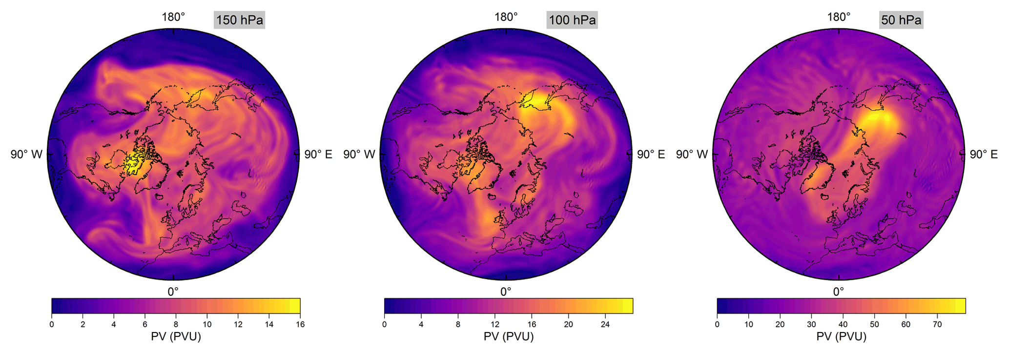
Figure 4Northern Hemisphere potential vorticity (PV) maps from ECMWF reanalysis at 150, 100 and 50 hPa on 26 February 2016 at 12:00 UTC. Note the different colour scales in each panel.

Figure 5 gives an overview of the temporal sampling of vortex air above different potential temperatures θ over the whole PGS campaign. Therefore, the number of individual (HCl) measurements during each flight is summed up and depicted in columns. The colour code indicates the vortex air encounters divided in measurements above a certain potential temperature. Extensive vortex air sampling was performed primarily at the end of the first main phase and during the second main phase, in concert with the gradual descent of higher vortex air masses to flight altitude. Specifically, vortex air encounters represent between 3 % and 95 % of flight time of individual flights. In situ sampling was focused on θ>340 K for most flights, keeping significant distance to the tropopause. Vortex air above θ=380 K was only sampled as of 26 February 2016 when mainly adiabatic transport brought air masses with such high potential temperatures within reach of the HALO aircraft. The 400 K isentrope was only crossed during three occasions in March with a total time of about 10 min inside vortex air.

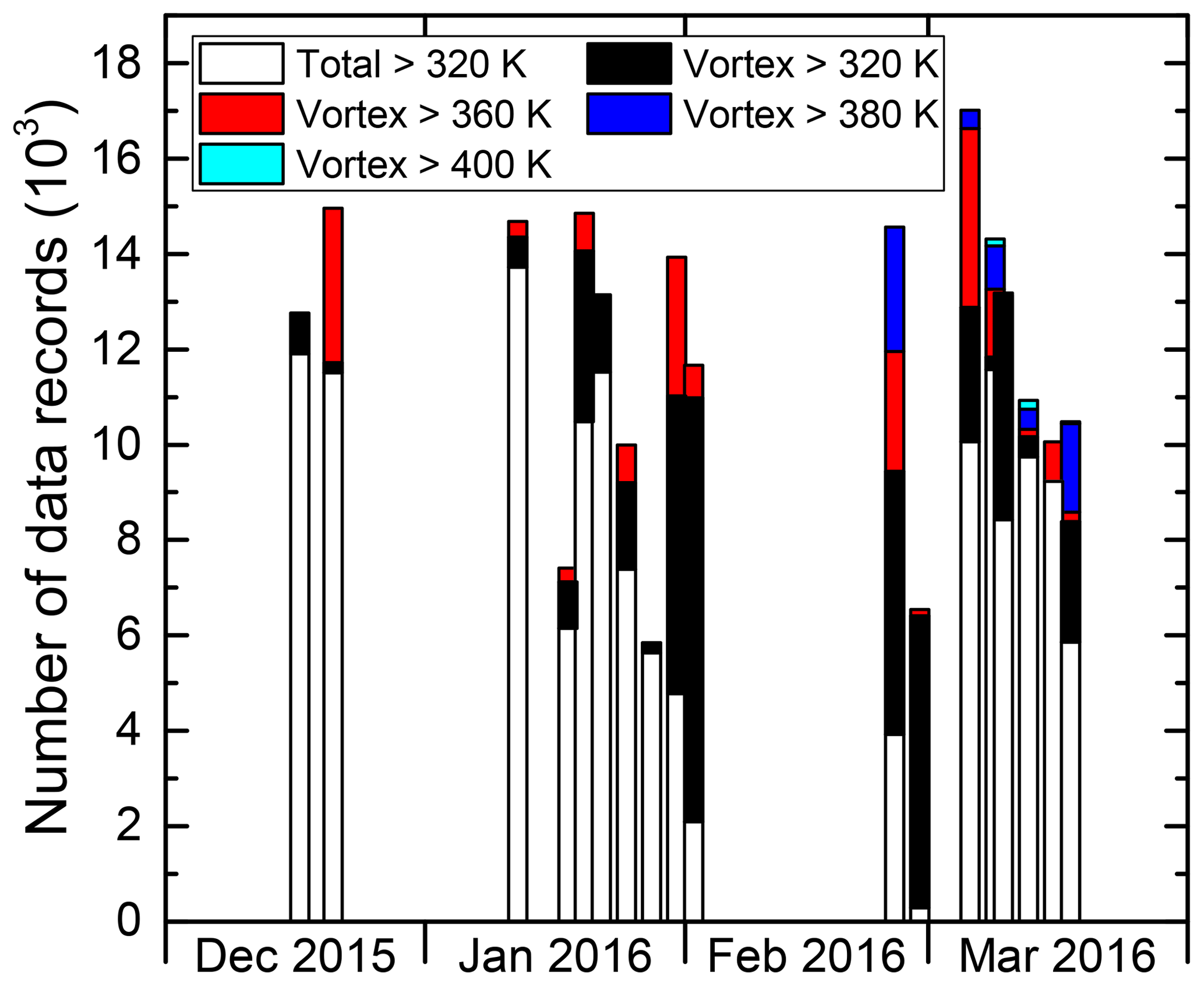
Figure 5Vortex air sampling statistics of the PGS campaign, counted by the number of individual HCl measurements. Each column represents a single science flight. Coloured bars indicate portions above selected isentropes.

Download

3.2 Measured evolution of chlorine gases during the winter

The evolution of inorganic chlorine partitioning in the lowermost Arctic polar vortex over a period of 3 months is assessed by means of daily statistics, which is performed by calculating averages, standard deviation and quantiles from all vortex air data points during individual research flights in order to get a reasonable statistical sample size. This allows the study of changes in trace gas concentrations on a timescale of days. Beforehand, the data are binned into four layers of potential temperature, each spanning 20 K, to introduce a coarse quasi-vertical coordinate. Panels (a)–(d) in Fig. 6 display the mean of the measured distributions for the individual HALO flights. Colours indicate the θ layers. The layer 320–340 K is omitted for clarity as it shows almost no difference to the 340–360 K layer. Panels (e)–(g) are similar to panels (a)–(c), but display the relative abundance with respect to Cl_y instead of absolute mixing ratios.

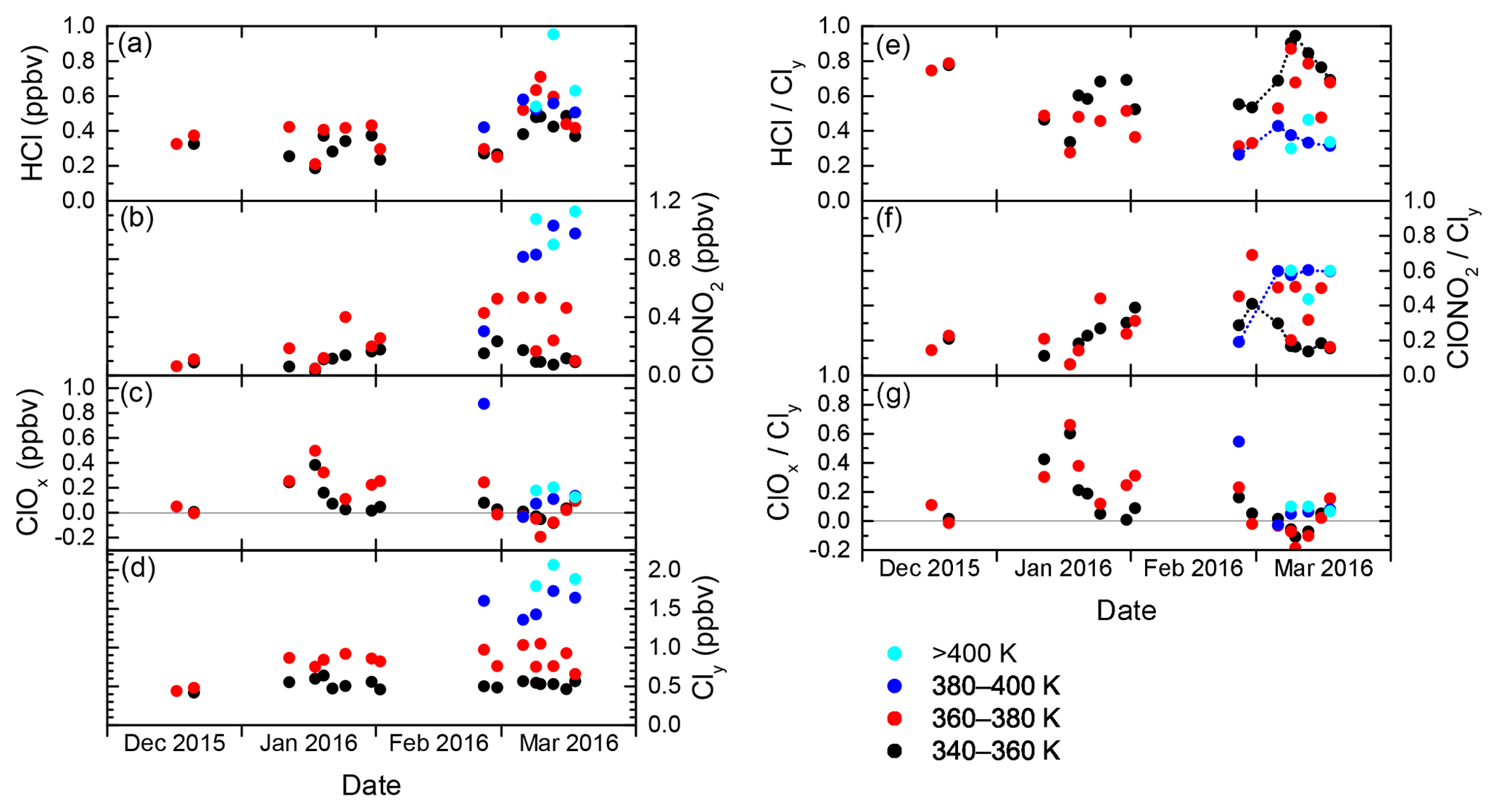
Figure 6Daily averages of measured mixing ratios of HCl, ClONO₂, ClO_x and Cl_y throughout the winter 2015/2016, from data that have been labelled “intra-vortex”. (a–d) Absolute mixing ratios. Colours are the same as in Fig. 5. (e–g) Similar to (a)–(d), but for relative contributions of HCl, ClONO₂ and ClO_x to Cl_y. Some of the black and blue points are connected by dashed lines to guide the eye along the different deactivation pathways.

Download

In December 2015, the measurements indicate that inorganic chlorine is partitioned almost entirely into the reservoir species HCl and ClONO₂ below the 380 K isentropic surface. With an almost 80 % contribution to Cl_y, the photochemically stable HCl is predominant, whereas ClONO₂ ranges with less than 0.12 ppbv below or near the detection limit. This ratio is common in unperturbed conditions (e.g. Santee et al., 2008). At this early stage of the polar vortex, no ClO_x has been detected.

The partitioning changes in January 2016, when the vortex is fully developed and temperatures are low enough to enable heterogeneous chemistry. The chlorine activation manifests itself in several ways in the observations: The absolute HCl mixing ratio does not show a general trend through early February below 380 K, but in terms of relative partitioning, HCl makes up a smaller fraction of the total Cl_y with respect to December conditions. In addition, HCl exhibits intermediate minima at the length of days with a decrease by up to 0.21 ppbv, as well as a final minimum on 2 February, that may indicate episodes of enhanced chlorine activation. The lowest HCl mixing ratio measured above 360 K is 0.17 ppbv on 20 January. Correspondingly, at least two phases of enhanced active chlorine can be identified, in mid- and late January and early February. On 18 January, measurements suggest that up to 75 % or 0.58 ppbv of Cl_y is activated below 380 K. These observations correspond with periods of high occurrence of ice and nitric acid trihydrate (NAT) PSCs (Voigt et al., 2018), which provide surfaces for heterogeneous chlorine activation. Enhanced mixing ratios of ClONO₂ up to 0.52 ppbv show how chlorine is repartitioned once sufficient amounts of ClO have been produced. The apparent rise in mean total Cl_y mixing ratio between December and January at 360–380 K from 0.44 to about 0.85 ppbv reflects the diabatic cooling that brings higher-level air masses to lower potential temperatures.

Large parts of the lower stratosphere could be sampled during the second main phase of the HALO deployment in late February and March, which covers the late stages of vortex evolution including the major final warming (MFW). The measurements show significant chlorine activation at the beginning of the second campaign phase when HALO could sample air masses above 380 K potential temperature for the first time, where a peak amount of 1.15 ppbv ClO_x at the flight altitude of 13 km was found. The MFW on 5 March (Manney and Lawrence, 2016) observably terminated heterogeneous chlorine activation reactions, with remaining ClO_x amounts no greater than 0.20 ppbv. The build-up of the reservoir species from deactivated compounds (sometimes referred to as “recovery”) varies strongly across the specified isentropic layers (supported by dashed lines in Fig. 6e–f): below 360 K, a gradual increase in HCl up to 0.58 ppbv throughout March can be seen, whereas ClONO₂ soon returns to concentrations below the detection limit. The stratospheric warming made higher θ levels accessible to HALO, and above 380 K, recovery pathways are different: depleted HCl starts to recover, but this positive trend is halted and eventually reversed by early to mid-March. Meanwhile ClONO₂ increases strongly above the level of HCl mixing ratios. Between 360 and 380 K (red data), observations are not very clear about the overall evolution, especially of ClONO₂. Also, negative values for ClO_x are calculated. While these are still within the uncertainty limits, this isentropic layer seems to contain a strong vertical variability of chemical constituents involved in chlorine repartitioning, communicating the different behaviour below and above. The vertical sampling of HALO may introduce a bias, which is also obvious in the enhanced variability of mean Cl_y values in the layers above 360 K. This is investigated further by the model intercomparison below.

Figure 7 illustrates the concept of differential deactivation pathways in this late winter period in a different manner. There, the partitioning of Cl_y is shown in a ternary diagram of HCl, ClONO₂ and ClO_x fractions. The dots mark individual measurements, the same that the daily averages in Fig. 6e–g were based on. The solid arrows run along the temporal evolution of the daily averaged measurements and show the two pathways below 360 K (black) and above 380 K (blue), diverging towards HCl or ClONO₂, as well as the 360–380 K isentropic layer (red) sandwiched in between. Using the supporting green isolines of the HCl∕ClONO₂ fraction, we observe that below 360 K, the partitioning between the reservoir species is more HCl-heavy and after recovery, HCl is 3 times more abundant than ClONO₂. Above 380 K, in contrast, the reservoir species evolve from a nearly 1:1 partitioning to a state with twice as much ClONO₂ relative to HCl.

Figure 7Ternary diagram of the partitioning of Cl_y into HCl, ClONO₂ and ClO_x during the second main campaign phase, from 26 February to 18 March 2016. The HCl isolines run from bottom left to top right, the ClONO₂ isolines horizontally and the ClO_x isolines from top left to bottom right. Dots mark individual measurements, where colours indicate the isentropic layers. Solid arrows illustrate the temporal evolution of the daily averages. As an aid to the reader, three green lines denote characteristic values of the HCl∕ClONO₂ ratio, and the orange dashed arrow points towards decreasing values of the ClO_x fraction.

Download

3.3 Comparison of measured and CLaMS-modelled data

Simulations by the Lagrangian chemistry transport model CLaMS were performed to put the observations into a broader context, and to investigate sampling biases potentially caused by the coverage of the aircraft observations. To assess the accuracy of the model, the model results were interpolated to the location and time of the observations employing the trajectory mapping described above. Figure 8 displays the model results (crosses) alongside the observations sampled with the same vortex criteria and averaging procedures. As for HCl, the model generally follows the trends of the measurement data. Before February, however, there is a clear high bias by 0.13–0.20 ppbv in almost all model HCl data which cannot be systematically seen after the break. Having ruled out technical changes to the simulation and to the instrumental sides during this time, it seems as if we can observe a model bias that is known from satellite comparisons at higher altitudes in the dark polar vortices, a problem that is observed by other models as well (Wohltmann et al., 2017; Grooß et al., 2018). Our intercomparison of model and in situ data supports the rationale that chemistry–climate models struggle in reproducing the observed chlorine partitioning in the dark winter months, where some unknown process for HCl removal is lacking. Here we extend the previous observations by Grooß et al. (2018) to lower altitudes. Consistently, the discrepancy is absent as soon as sufficient sunlight returns towards the end of the winter. An overestimation of HCl is partly reflected in an overestimation of Cl_y and underestimated ClONO₂ and ClO_x concentrations.

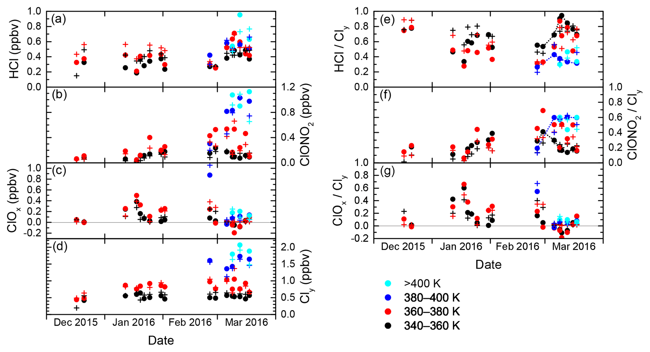
Figure 8Similar to Fig. 6. In addition to averages from the measurements depicted as points, crosses denote averages from CLaMS model data interpolated at the flight track.

Download

ClONO₂ is better represented in the model below θ=360 K, whereas there are indications of a slight underestimation at higher potential temperatures. This may be induced in part by the HCl high bias until midwinter, or by generally underestimated Cl_y mixing ratios recognizable above 380 K. The model is able to produce the observed change in recovery across the different isentropes. The modelled vertical shift from HCl to ClONO₂ as the dominant reservoir species during repartitioning in March between 360 and 400 K is obviously subject to a sampling bias just like the measurements, but at the same time does not always follow the observational data. This deviation is probably caused by a lack of vertical resolution in the meteorological data fields that prevents the model from estimating the high vertical gradients in the atmosphere in all detail.

Beyond this direct intercomparison, model data can help explore to what extent the observations along the aircraft's flight track are representative of the entire polar vortex. Therefore, the lines in Fig. 9 display the modelled concentration of the chlorine species in a vortex-wide average at the different isentropic levels. In general the local aircraft observations reflect the mean chlorine partitioning in the vortex LMS quite well. The periods when activated chlorine can be found are consistent, whilst enhanced local variation in ClO_x in January is not projected into the vortex averages. Vortex-averaged HCl mixing ratios clearly suffer from the deviation during the dark episode. Toward the end of the winter, the vortex averages include air masses from lower latitudes at increased frequency. This is accompanied, for example, by a sudden drop in modelled mean ozone (not shown), which would explain the lower values of all chlorine species, compared to the measurements in the local remainders of vortex air.

Figure 9Similar to Figs. 6 and 8. In addition, lines represent whole vortex model averages.

Download

3.4 Variability of chlorine partitioning

To assess the validity of using daily averaged mixing ratios as in the previous sections, Fig. 10 displays, in addition to mean values, the extrema and quartiles from the statistics studied hitherto, where the 360–380 K layer is taken as an example that stretches over all measurement phases. Intermediate data spread, as seen in most January flights, reflects the small and steady variation through the depth of the layer, while trends between consecutive flights are clearly visible. There, the statistics are based on a solid sample size, and these are the periods where measurements and model data match best. A very low variability, such as for the first December flight or for two flights on 10 and 13 March, stems from very few vortex sampling points in this layer, rendering these values less representative. Consistently, the model data interpolated along the flight track deviates the strongest from the measurements on these dates, as visible in the HCl and ClONO₂ results. Very high variability, as seen on 26 February and 6 March, hints at enhanced differential processing or transport within the sampled air masses.

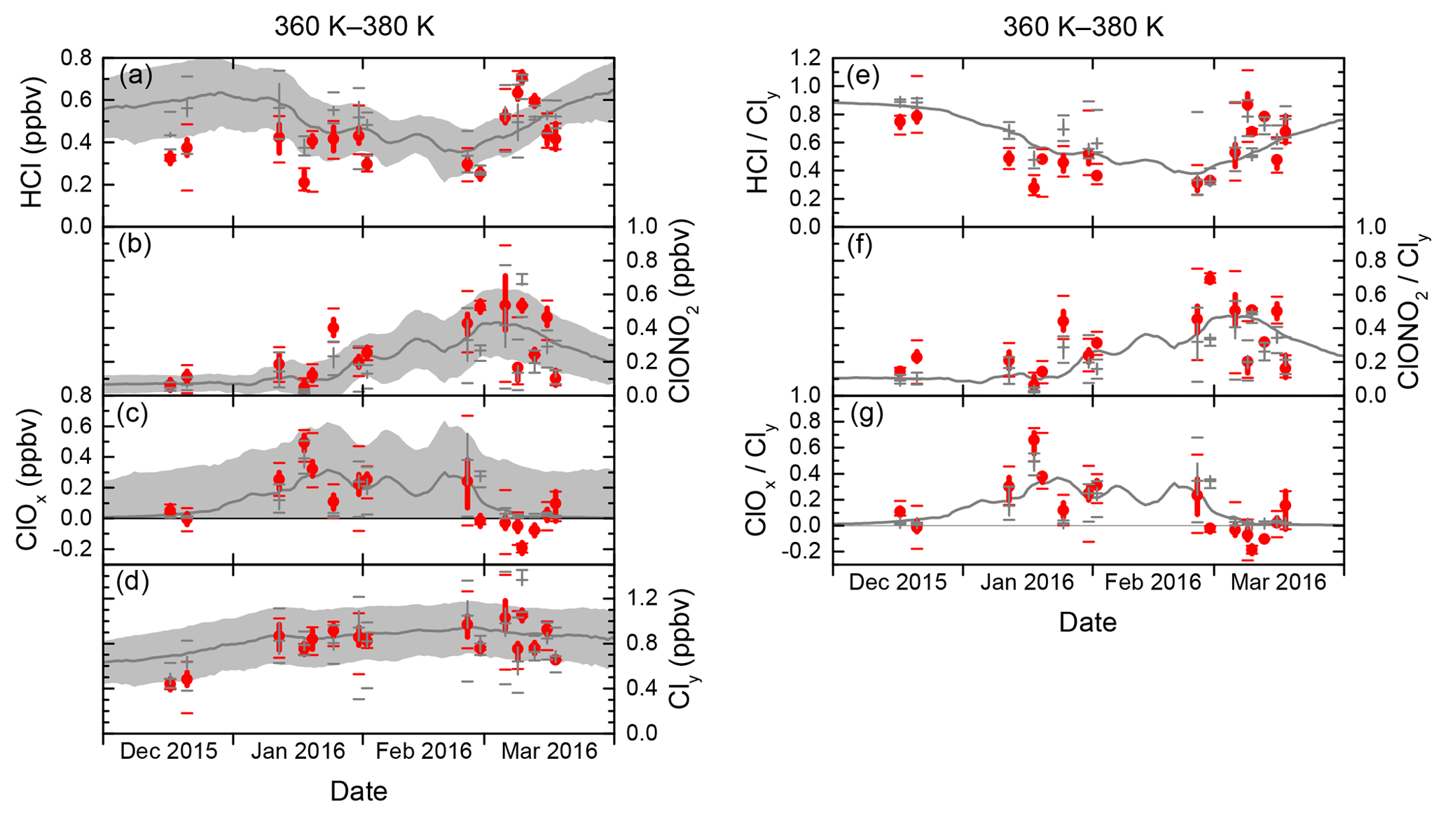
Figure 10Similar to Fig. 9, with more detailed statistics of only the 360–380 K layer. Measurements are red, and model data are grey. Beyond the mean values (points and crosses), vertical bars span the second and third quartiles, while horizontal bars indicate minimum and maximum values. The grey area encompasses the standard deviation from the vortex averaging (only for panels a–d).

Download

The standard deviation of the vortex-averaged statistics (grey shading in Fig. 10a–d) reflects the intra-vortex atmospheric variability. Without accounting for potential systematic biases, two-thirds or 67 % of the observational data are found within this spread, which demonstrates the joint performance of the measurements and the model at reproducing vortex air characteristics on single aircraft flight tracks.

3.5 Discussion

In this section, our observed evolution of chlorine partitioning during the winter 2015/2016 is compared to previous studies using in situ and remote-sensing data.

The Arctic polar vortex during winter 2015/2016 has been studied by Manney and Lawrence (2016), using measurements from the Aura MLS instrument. As for chlorine species, they retrieved HCl and ClO at a vertical resolution of 2.5–6 km down to θ=390 K. Therefore, the satellite data only have a small overlap with our in situ observations in March. Nevertheless, the depletion and recovery of HCl, as well as the occurrences of active chlorine, as reported in Sect. 3.2, consistently extend the remote-sensing observations to lower altitudes, and show that chlorine activation is generally not limited to the higher altitudes inside the Arctic polar vortex.

Based on measurements on the ER-2 aircraft within the SOLVE/THESEO mission, Wilmouth et al. (2006) drew a very comprehensive picture of inorganic chlorine partitioning in the Arctic polar vortex of 1999/2000, where low temperatures (Manney and Sabutis, 2000), high PSC presence and large chemical ozone loss (Rex et al., 2002) were observed. At isentropes around 440 K, ClO_x∕Cl_y reached up to 90 % in January and HCl accounted for the remaining 10 %, whereas ClONO₂ was not detectable. Thus, the higher degree of activation at higher potential temperatures, compared to the PGS measurements, seems to come mainly at the expense of ClONO₂. From their late winter budget analysis, Wilmouth et al. (2006) suggest that HCl recovers at a rate similar to or higher than the ClONO₂ recovery rate. They state that the evolution of inorganic chlorine partitioning in the Arctic is rather variable. Whether the chlorine deactivation into ClONO₂ or HCl is favoured depends critically on the mixing ratios of ozone and NO_x (Grooß et al., 2005). Our late winter measurements are in line with observations during a balloon sounding of MIPAS-B (Michelson Interferometer for Passive Atmospheric Sounding) and TELIS (TErahertz and submillimeter LImb Sounder) in the late Arctic winter 2011 (Wetzel et al., 2015). There, HCl is the dominant reservoir species below 14 km altitude, while the ratio is shifted towards ClONO₂ between 14 and 24 km. In an overview of stratospheric polar winter chlorine partitioning by Santee et al. (2008), based on MLS and ACE-FTS satellite data, observations at θ=500 K in different years show different late winter patterns. In 2004/2005 in the Arctic, chlorine is mainly deactivated by ClONO₂ formation, which rises to about 60 % at the end of the winter, similar to our observations above 380 K. Only later is chlorine slowly repartitioned into HCl through ClONO₂ photolysis towards the unperturbed conditions. The Arctic winter 2005/2006, instead, reveals a much faster build-up of HCl, similar to what Wilmouth et al. (2006) report and what is more reminiscent of the Antarctic stratosphere.

The general year-to-year variability in the northern hemispheric polar vortex is caused by high wave activity, which impacts the stability of the vortex and resultant cooling that occurs. On the process scale, the tradeoff between HCl or ClONO₂ recovery is controlled by the availability of reaction partners. NO₂ is needed for ClONO₂ formation, and may be introduced through mixing at the vortex edge (e.g. Krause et al., 2018), or through photolysis of gaseous HNO₃. HCl recovery is favoured if low ozone leaves enough Cl radicals to react with methane, which is typically the case in the lowermost stratosphere.

The same instruments used in the present study were previously used for measurements in the Antarctic polar vortex on 13 September 2012 at isentropes between 320 and 385 K (Jurkat et al., 2017), where up to 40 % active chlorine was observed. Both the Arctic and Antarctic aircraft observations were made at (static) temperatures above 199 K, often even above 210 or 220 K. This is too warm for PSCs and for heterogeneous processes. Therefore, observable ClO_x must have been activated beforehand, potentially with subsequent downward transport. This shows that, in both hemispheres, active chlorine can remain present in the vicinity of regions with temperatures below the PSC threshold.