Finding reconnection lines and flux rope axes via local coordinates in global ion-kinetic magnetospheric simulations

Alho, Markku; Cozzani, Giulia; Zaitsev, Ivan; Kebede, Fasil Tesema; Ganse, Urs; Battarbee, Markus; Bussov, Maarja; Dubart, Maxime; Hoilijoki, Sanni; Kotipalo, Leo; Papadakis, Konstantinos; Pfau-Kempf, Yann; Suni, Jonas; Tarvus, Vertti; Workayehu, Abiyot; Zhou, Hongyang; Palmroth, Minna

doi:https://doi.org/10.5194/angeo-42-145-2024

Articles | Volume 42, issue 1

https://doi.org/10.5194/angeo-42-145-2024

Articles | Volume 42, issue 1

Regular paper

16 May 2024

Regular paper |

| 16 May 2024

Finding reconnection lines and flux rope axes via local coordinates in global ion-kinetic magnetospheric simulations

Markku Alho, Giulia Cozzani, Ivan Zaitsev, Fasil Tesema Kebede, Urs Ganse, Markus Battarbee, Maarja Bussov, Maxime Dubart, Sanni Hoilijoki, Leo Kotipalo, Konstantinos Papadakis, Yann Pfau-Kempf, Jonas Suni, Vertti Tarvus, Abiyot Workayehu, Hongyang Zhou, and Minna Palmroth

Abstract

Magnetic reconnection is a crucially important process for energy conversion in plasma physics, with the substorm cycle of Earth's magnetosphere and solar flares being prime examples. While 2D models have been widely applied to study reconnection, investigating reconnection in 3D is still, in many aspects, an open problem. Finding sites of magnetic reconnection in a 3D setting is not a trivial task, with several approaches, from topological skeletons to Lorentz transformations, having been proposed to tackle the issue. This work presents a complementary method for quasi-2D structures in 3D settings by noting that the magnetic field structures near reconnection lines exhibit 2D features that can be identified in a suitably chosen local coordinate system. We present applications of this method to a hybrid-Vlasov Vlasiator simulation of Earth's magnetosphere, showing the complex magnetic topologies created by reconnection for simulations dominated by quasi-2D reconnection. We also quantify the dimensionalities of magnetic field structures in the simulation to justify the use of such coordinate systems.

Download & links

How to cite.

Alho, M., Cozzani, G., Zaitsev, I., Kebede, F. T., Ganse, U., Battarbee, M., Bussov, M., Dubart, M., Hoilijoki, S., Kotipalo, L., Papadakis, K., Pfau-Kempf, Y., Suni, J., Tarvus, V., Workayehu, A., Zhou, H., and Palmroth, M.: Finding reconnection lines and flux rope axes via local coordinates in global ion-kinetic magnetospheric simulations, Ann. Geophys., 42, 145–161, https://doi.org/10.5194/angeo-42-145-2024, 2024.

Received: 09 Oct 2023 – Discussion started: 23 Oct 2023 – Accepted: 14 Feb 2024 – Published: 16 May 2024

1 Introduction

A long-standing issue in analysing data from magnetospheric simulations has been the identification of topological features in the magnetic field, especially in relation to reconnection and flux transfer events. These features include magnetic neutral lines; separators; and, loosely, X and O lines. In a 2D configuration, the problem is tractable via the use of a flux function (see Sonnerup, 1970, for an early example, with details given in, for example, Servidio et al., 2009). Recent examples of flux function use include Hoilijoki et al. (2017), Palmroth et al. (2017) and Hoilijoki et al. (2019). A generalized flux function can be defined in certain 3D configurations (Yeates and Hornig, 2011). Global ideal magnetohydrodynamic (MHD) simulations present a relatively simple reconnection topology that is tractable via the four-field junction (FFJ) method that identifies reconnection topologies from global magnetic field connectivity (whether or not field lines connect to Earth or to the solar wind) (Laitinen et al., 2006). However, more detailed simulations, such as Vlasiator ion-kinetic simulations, produce complex reconnection topologies impossible for FFJ to parse completely (see Pfau-Kempf et al., 2020). As such, the space physics community is challenged to find and develop new tools for analysing these topologies.

Reviewing the definitions of the topological structures of reconnecting 3D magnetic fields by Parnell et al. (2010), we can summarize three different but related concepts: magnetic null points (with several subtypes), where the magnetic field B completely vanishes; separatrices (also called separator surfaces or separatrix surfaces), which are planes that delimit different magnetic domains; and separators, which are lines connecting magnetic null points, defined as intersections of paired separatrix surfaces lying at the boundary of four different magnetic domains. The behaviour of magnetic null points has been studied in much detail – in 3D as well (e.g. Greene, 1988) – for their usefulness in reconnection analysis. Detection and classification of null points can be done readily with existing methods: Olshevsky et al. (2015, 2016) use the Poincaré index method to detect and characterize null points (where B(r)=0) in local MHD and particle-in-cell (PIC) simulations, which can be applied to spacecraft data as well. Haynes and Parnell (2007) detail methods of finding null points within a cubic cell, using a tri-linear method to find common zero-crossings for all magnetic field components. Fu et al. (2015) introduced the first-order Taylor expansion (FOTE) method for reconstructing the magnetic field topology around nulls and finding null points from multi-point spacecraft data.

As, for example, Lau and Finn (1990) note that the magnetic field lines connecting specific null-point pairs – separators – are important for reconnection. For example, Dorelli and Bhattacharjee (2009) discuss topological changes in dayside separators during flux transfer event (FTE) formation in MHD simulations. Several methods for finding separator lines have been developed. For example, Komar et al. (2013) trace related separators by stepping from magnetic null points and inspecting magnetic connectivity of candidate points, which is akin to the FFJ method used by Laitinen et al. (2006). This is used by Eggington et al. (2022) to find the main magnetospheric separator through tracing magnetic connectivity; it is noted that they found it complicated to find the initial magnetic nulls for tracing. On the other hand, Olshevsky et al. (2016) show a plethora of null points found in a magnetospheric simulation, representing a challenge for mapping the pairwise connections of null points. Glocer et al. (2016) track magnetic separators in MHD simulations and compare different techniques for it, while Haynes and Parnell (2010) introduced generalized methods for constructing the topological skeletons of magnetic fields. This includes null points, separatrices and the separator lines, not tied to specific coordinate systems, with involved field line tracing procedures. Recently, Bujack et al. (2021) also introduced similar tools. Such tools are likewise being explored in Vlasiator 3D magnetospheric simulations by Bouri et al. (2023) in order to apply machine learning methods to the topic. Machine learning methods have also seen use in the analysis of plasma simulations by, for example, Bussov and Nättilä (2021).

Closely related to the concept of separators are the magnetic X and O lines. As the intersections of separatrix surfaces, the separators delimit different magnetic domains. In the classic picture of reconnection, inspecting the magnetic field lines on a plane normal to the tangent of the reconnection line displays an X topology, with the in-plane components of B changing signs at the X line (or an X point when constrained to such a plane). This holds regardless of an out-of-plane B component, as noted by Parker (1957) and Sonnerup (1974): the hyperbolic structure remains visible in the in-plane components. Likewise, the in-plane magnetic field components change signs at an O line (or O point). This can be used to extend the definition from a true null line, defined as a continuous line with exactly zero B, which is structurally unstable (Priest and Titov, 1996) and is expected to split into null points connected by a separator. As this definition of a null line is not consequently fulfilled in practice and because we would like to identify null lines whether or not a magnetic guide field is present, we use the term in-plane null line (and, more specifically, in-plane X and O lines) in this paper to mean such sets of points that satisfy the zero-crossing condition for the in-plane magnetic field components, allowing for a common category of null lines that covers both X and O lines, with and without guide field. It should be noted, however, that the notion of an in-plane null depends on the definition of the plane, and it is not clear what plane should be chosen for this decomposition. This work proposes one possible selection of a useful coordinate system via variance analysis for this purpose. Other selections of a coordinate system are possible, as shown by, for example, Genestreti et al. (2018).

For magnetic field structures such as current sheets (CSs), null lines and flux ropes, it is useful to select a suitable coordinate system that can exploit the properties of the structure to simplify the problem at hand. Methods such as minimum variance analysis (MVA, Sonnerup and Scheible, 1998) are widely used in spacecraft observational studies to investigate structures in amenable coordinate systems (Paschmann and Daly, 1998). Observational methods for the construction of local coordinate systems may require some situational adjustments, as in Gosling and Phan (2013) and Hietala et al. (2018), with a hybrid MVA coordinate system. Indeed, Genestreti et al. (2018) examine 14 different variations of generating local coordinate systems for a reconnection event observed by the Magnetospheric Multiscale (MMS) mission. The magnetic field structures that are more frequently investigated (such as CSs and flux ropes) often display more variability in some dimensions than in others, allowing for some simplifications based on the dimensionality of the structures. Methods for inspecting the dimensionality and for forming local coordinate systems are reviewed by Shi et al. (2019). Particularly, the minimum directional derivative (MDD) and minimum gradient analysis (MGA) methods may be used to define local coordinate systems based on the Jacobian of the magnetic field B, which we will build upon in this work. These are detailed in Sect. 1.1.

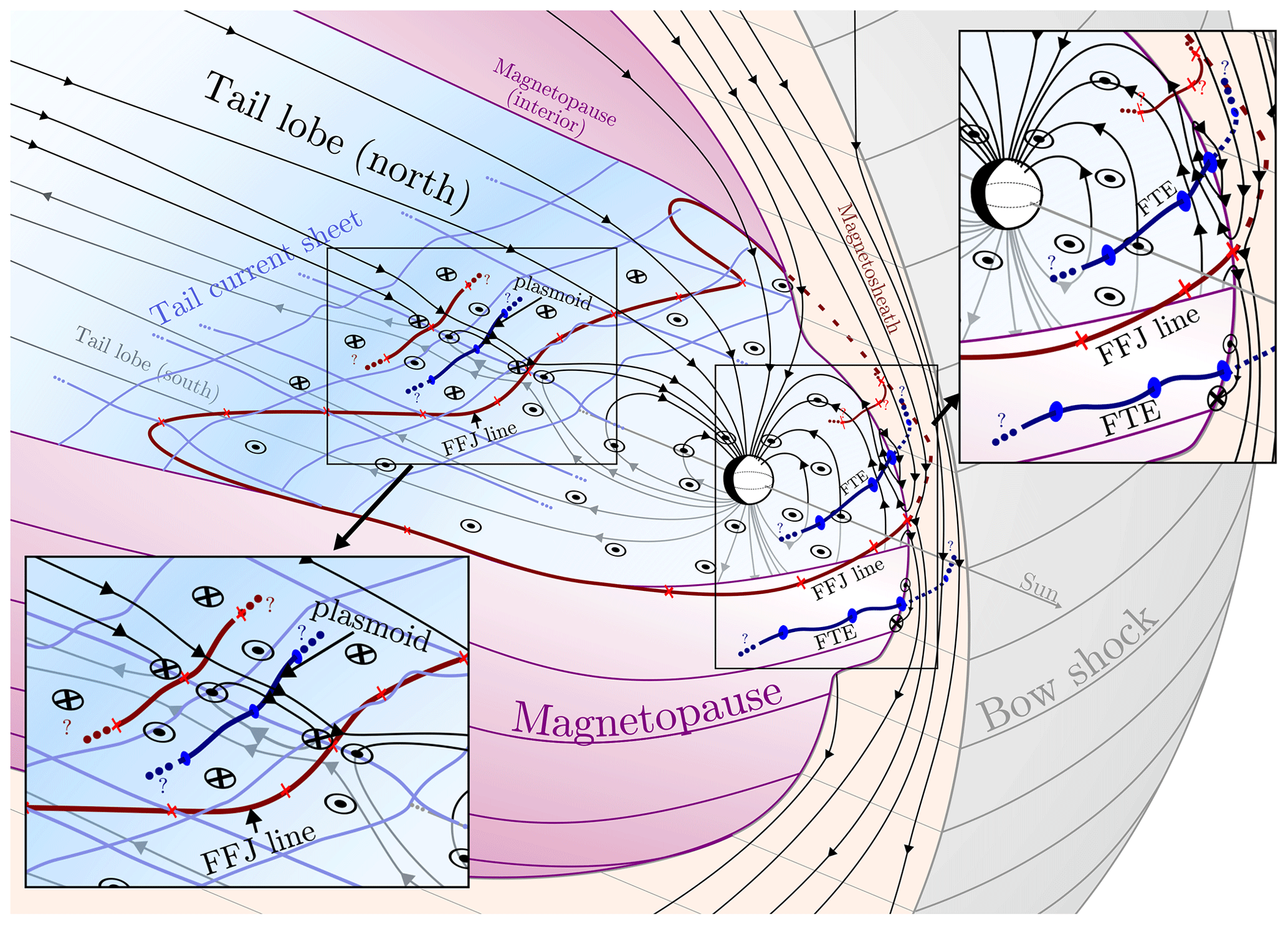
https://angeo.copernicus.org/articles/42/145/2024/angeo-42-145-2024-f01

Figure 1A schematic view of Earth's magnetosphere under southward-IMF driving, with zoomed-in detail panels of the dayside magnetopause and the magnetotail, sketched on the Vlasiator run described by Palmroth et al. (2023). The magnetosphere proper is delimited by the magnetopause (purple surface). Magnetic field lines on the meridional plane are shown in black, with X (red, crosses; global FFJ line annotated) and O (blue, discs; marked with FTE and plasmoid) topologies marked as lines close to the meridional plane (and one X topology circling the near-Earth region with a northward magnetic field). The white and light-blue equatorial cross section follows the magnetic Equator and the tail current sheet, with the north–south magnetic field marked, respectively, as out of and into the plane.

Download

Global magnetospheric simulations use global coordinate systems such as the Geocentric Solar Ecliptic (GSE) or Geocentric Solar Magnetospheric (GSM) systems, similarly to spacecraft observations. However, local magnetic structures are not necessarily aligned with the axis of the simulation coordinate system. In particular CSs, flux ropes and reconnection topologies can develop unconstrained by the domain boundaries and can be oriented in virtually any direction. In this situation, methods developed to analyse spacecraft data can inspire new ways to investigate data from global simulations. Palmroth et al. (2023) used justified assumptions about the geometry of the problem to obtain useful proxies from global coordinate systems, and the aim of this paper is to generalize the approach to a local coordinate system.

To review our region of interest, Fig. 1 shows a sketch of Earth's magnetosphere based on the Vlasiator simulation described by Palmroth et al. (2023). Solar wind flows in from the right, carrying with itself the interplanetary magnetic field (IMF), which is aligned purely southward in this simulation. As the solar wind encounters Earth's magnetic field, a bow shock (grey) and a heated magnetosheath (light brown) are formed (both are shown clipped along the meridional plane). The magnetopause (purple, clipped along the equatorial plane) delimits the magnetosphere proper: the volume in which Earth's magnetic field dominates the plasma behaviour. The solar wind driving draws the magnetosphere into a long tail, with northern and southern tail lobes having opposite magnetic fields and with the tail current sheet (CS, light blue) separating the lobes. Southward IMF driving is especially interesting as it allows for magnetic reconnection on the dayside magnetopause, where the opposing magnetic fields form X topologies (dark-red lines with crosses) and allow for the transfer of energy and mass across the magnetopause and a change in global magnetic topology. The global reconnection line described by Laitinen et al. (2006) is correspondingly shown as the closed, dark-red line marked as FFJ. The reconnected magnetic field lines form flux transfer events (FTEs or plasmoids) characterized by O topologies (blue lines with discs). Similarly, the opposing magnetic fields of the tail lobes may reconnect at the tail CS, forming plasmoids in the tail current sheet. Palmroth (2023) shows complex reconnection topologies that form in the tail, represented by the ellipsis-terminated red and blue lines in the tail of Fig. 1, with similar sketches of multiple reconnection lines and flux transfer events given on the dayside magnetopause.

https://angeo.copernicus.org/articles/42/145/2024/angeo-42-145-2024-f02

Figure 2Schematic drawing of the (a) MGA and (b) MDD eigenvectors $\hat{L}, \hat{M}$ and $\hat{N}$ , corresponding to the largest, middle and minimum eigenvalues in a 1D CS, along the lines of Shi et al. (2019). For both eigensystems, the vector $\hat{L}$ is well-defined, while the $\hat{M}$ and $\hat{N}$ vectors lie on the plane perpendicular to the $\hat{L}$ vectors.

Download

In this paper we introduce and discuss alternative, physically motivated local methods for finding X and O lines in the magnetic field of global 3D magnetospheric simulations by inspecting the magnetic field on a suitable local coordinate basis. To extend the global proxies used in Palmroth et al. (2023), we introduce a local coordinate system based on the work reviewed by Shi et al. (2019), with an approach similar to the one presented by Denton et al. (2010), and describe both contouring and cell-wise FOTE methods for finding null lines, both X and O, within a global magnetospheric plasma simulation based on the magnetic field and its Jacobian matrix.

1.1 Local coordinate systems and dimensionality

Let us consider two methods reviewed by Shi et al. (2019): minimum directional derivative (MDD) and minimum gradient analysis (MGA, analogous to minimum variance analysis), both defined using the Jacobian G=∇B of the magnetic field. Local, orthogonal coordinate directions can be obtained from the eigenbases of G^⊺G (MGA) and GG^⊺ (MDD). However, as these methods obtain the initial directions as eigenvectors that are defined up to a real scalar, the directions (after normalization) are defined up to a factor of ± 1.

MGA produces a set of basis vectors where the eigenvector that corresponds to the largest eigenvalue (λ₁) is aligned with the vector that has maximal variation ( ${\hat{L}}_{MGA}$ ), the second one (λ₂) corresponds to the intermediate variation ( ${\hat{M}}_{MGA}$ ), and the third (λ₃) corresponds to the least variation ( ${\hat{N}}_{MGA}$ ). On the other hand, the MDD method produces a set of basis vectors where the eigenvector corresponding to the largest eigenvalue shows the direction of the displacement which produces the largest variation in B ( ${\hat{L}}_{MDD}$ ). Correspondingly, for the eigenvectors corresponding to the intermediate and least eigenvalues we use ${\hat{M}}_{MDD}$ and ${\hat{N}}_{MDD}$ . Denton et al. (2010) employ the MDD eigenbasis in their method, while we use both MDD and MGA eigenvectors, as described later in Sect. 2.1.

Both of these eigensystems have the same eigenvalues, but the eigenvectors differ and are not necessarily aligned with each other. We note here that, for a 1D structure, both of these eigensystems have only one well-defined eigenvector. For example, in a 1D Harris (1962)-type CS defined by

\begin{matrix} (1) & B (z) = B_{0} \tanh (z) \hat{x} \end{matrix}

for some constant B₀, the eigensystems are shown in Fig. 2, with ${\hat{L}}_{MGA}$ being aligned with $\hat{x}$ and ${\hat{L}}_{MDD}$ being aligned with $\hat{z}$ .

MDD also gives us a way to define the local dimensionality of a structure (Rezeau et al., 2018) from the eigenvalues of the matrix GG^⊺, with, for example, a purely 1D structure varying only as a function of a single coordinate. The quantities D₁, D₂ and D₃ describe the one-, two- and three-dimensionalities of the magnetic field and are obtained from the ratios of square roots of the eigenvalues $λ_{1} \geq λ_{2} \geq λ_{3}$ of GG^⊺.

Definitions for D₁, D₂ and D₃ are given below, modified to use the square roots of eigenvalues, as suggested by Shi et al. (2019) (as the square roots of the eigenvalues are then in units of T m⁻¹):

\begin{matrix} (2) & D_{1} = \frac{\sqrt{λ_{1}} - \sqrt{λ_{2}}}{\sqrt{λ_{1}}}, \\ (3) & D_{2} = \frac{\sqrt{λ_{2}} - \sqrt{λ_{3}}}{\sqrt{λ_{1}}}, \\ (4) & D_{3} = \frac{\sqrt{λ_{3}}}{\sqrt{λ_{1}}} . \end{matrix}

These quantities are defined to lie in the range [0,1], and their sum is 1. For D₁≈1, the magnetic field structure is primarily 1D, such as with a CS with B≈B(z) for a direction z normal to the CS. Correspondingly, for D₂≈1, the structure is primarily a function of two coordinates and so on. These measures allow us to quantify whether or not the local 2D treatment for neutral lines is well-founded, and we return to the topic of dimensionality in Sect. 4.3.

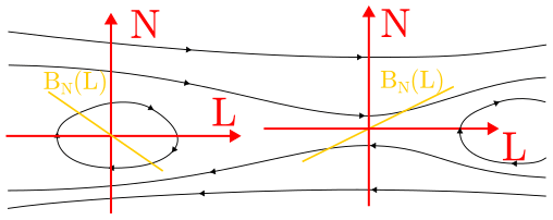
https://angeo.copernicus.org/articles/42/145/2024/angeo-42-145-2024-f03

Figure 3Neutral point classification in a well-defined local coordinate system. On the plane where B_L=0 and on the subset of that plane where B_N=0, the O points have $\partial B_{N} / \partial L < 0$ , and the X points have $\partial B_{N} / \partial L > 0$ . Note that this classification assumes a right-handed coordinate system.

Download

1.2 Vlasiator

In this study, the methods discussed above will be applied to a global simulation of Earth's magnetosphere performed with the hybrid-Vlasov code Vlasiator. Vlasiator is a supercomputer-scale 6D (3D+3V – three spatial dimensions and three velocity-space dimensions) ion-hybrid plasma simulation (von Alfthan et al., 2014; Palmroth et al., 2018), solving the Vlasov equation for ion components and treating electrons as a charge-neutralizing, massless fluid. Previously, Vlasiator has been used to study reconnection in 5D (2D+3V) simulations for the global magnetosphere (e.g. Hoilijoki et al., 2017; Palmroth et al., 2017) and locally in the magnetopause in full 6D (Pfau-Kempf et al., 2020). Recently, computational advances (Ganse et al., 2023) have expanded the capabilities of the model to include fully 6D global simulations (Palmroth et al., 2023; Horaites et al., 2023; Grandin et al., 2023).

We use the global Vlasiator simulation described by Palmroth et al. (2023) as a prototype case for the discussed methods. The simulation is of Earth's global magnetosphere, with an approximate conducting-sphere inner boundary condition that does not include ionospheric coupling. The simulation uses the GSE coordinate system (centred on Earth, with the x axis pointing towards the Sun, while the z axis is normal to the ecliptic in the northward direction) and no dipole tilt; thus, the dipole moment is aligned with the z axis. The simulation is set up with a predefined mesh refinement with 1000 km maximum spatial resolution in the tail CS and on the dayside magnetopause, with the simulation domain spanning $[- 111, 50] R_{E}$ in the X direction and $[- 58, 58] R_{E}$ in the Y and Z directions, with driving provided by the fast (U_sw = 750 km s⁻¹) solar wind at the temperature of T_sw = 500 kK and the density of n_sw = 1 cm⁻³ at the inflow boundary and a purely southward magnetic field B_IMF = $(0, 0, - 5)$ nT. Other boundaries employ copy conditions. The initial condition for the simulation is comprised of the velocity distribution functions initialized to Maxwellian distributions, with moments at the inner boundary set to a density of 1 cm⁻³ and a temperature of 5 × 10⁵ K with zero velocity; these distributions are smoothly tapered to solar wind values until the geocentric distance of 15.7 R_E (Horaites et al., 2023).

Despite the solar wind and IMF being constant, the kinetic physics involved in the simulation still produce a remarkably dynamic environment. Palmroth et al. (2023) described the dynamics of tail reconnection in the Vlasiator run, showing the interplay of plasma instabilities and reconnection on the tail CS. Notably, they presented a complex picture of small, independent plasmoids being generated in a bursty fashion, followed by a tail-wide reconfiguration through the merging of smaller plasmoids and their reconnection lines. Notably, the simulation setup is an idealized case, and with more realistic solar wind and IMF inputs, including a flow-aligned IMF component, dipole tilt and magnetosphere–ionosphere coupling, we expect to see even more complex behaviour, including, for example, tilted CSs (see e.g. Shen et al., 2008).

2 Methods: applying the local coordinate systems to Vlasiator

2.1 Local LMN coordinates

If the eigenvalues are not well-separated, the directions obtained from MGA and MDD may be ambiguous (see Shi et al., 2019). For example, for the CS with dimensionality 1, MGA obtains the field-aligned direction (above and below the CS), while MDD obtains the normal direction in relation to the CS, with two other directions being potentially ambiguous. The directions obtained from MGA and MDD are, however, approximately orthogonal at the CS. Since we are especially interested in CS-like structures, we choose to use the unit vectors ${\hat{L}}_{MGA}$ and ${\hat{L}}_{MDD}$ (described in Sect. 1.1) as the basis on which to build our coordinate system.

The electric current density $J \propto \nabla \times B$ can be used to define a right-handed coordinate system by selecting ${\hat{L}}_{MGA}$ as a primary vector $\hat{L}$ , ${\hat{L}}_{MDD}$ as a secondary vector and J as a tertiary vector so that $\hat{L} \times J ∥ {\hat{L}}_{MDD}$ . For example, on an idealized CS (Eq. 1), we see that $\hat{L} ∥ \hat{x}$ , $\hat{N} ∥ \hat{z}$ , and $J ∥ \hat{L} \times \hat{N}$ . $\hat{L}$ and ${\hat{L}}_{MDD}$ are exactly orthogonal in this case, as in Fig. 2.

To summarize the definition of our local LMN coordinate system $\hat{L}, \hat{M}, \hat{N}$ , we orthogonalize the set of basis vectors with the following:

$\hat{L} = {\hat{L}}_{MGA}$ .
$\hat{N} = {\hat{L}}_{MDD} - ({\hat{L}}_{MDD} \cdot \hat{L}) \hat{L}$ , with $\hat{N}$ multiplied by −1, if necessary so that $(\hat{N} \times \hat{L}) \cdot J > 0$ .
Lastly, $\hat{M} = \hat{N} \times \hat{L}$ .

The above results in a right-handed coordinate system with $\hat{M}$ oriented in the same direction as J (but not necessarily parallel). This still only requires data from G and allows for a classification of a null line in relation to X and O in this LN plane via inspection of $\partial B_{N} / \partial L$ (see Fig. 3).

https://angeo.copernicus.org/articles/42/145/2024/angeo-42-145-2024-f04

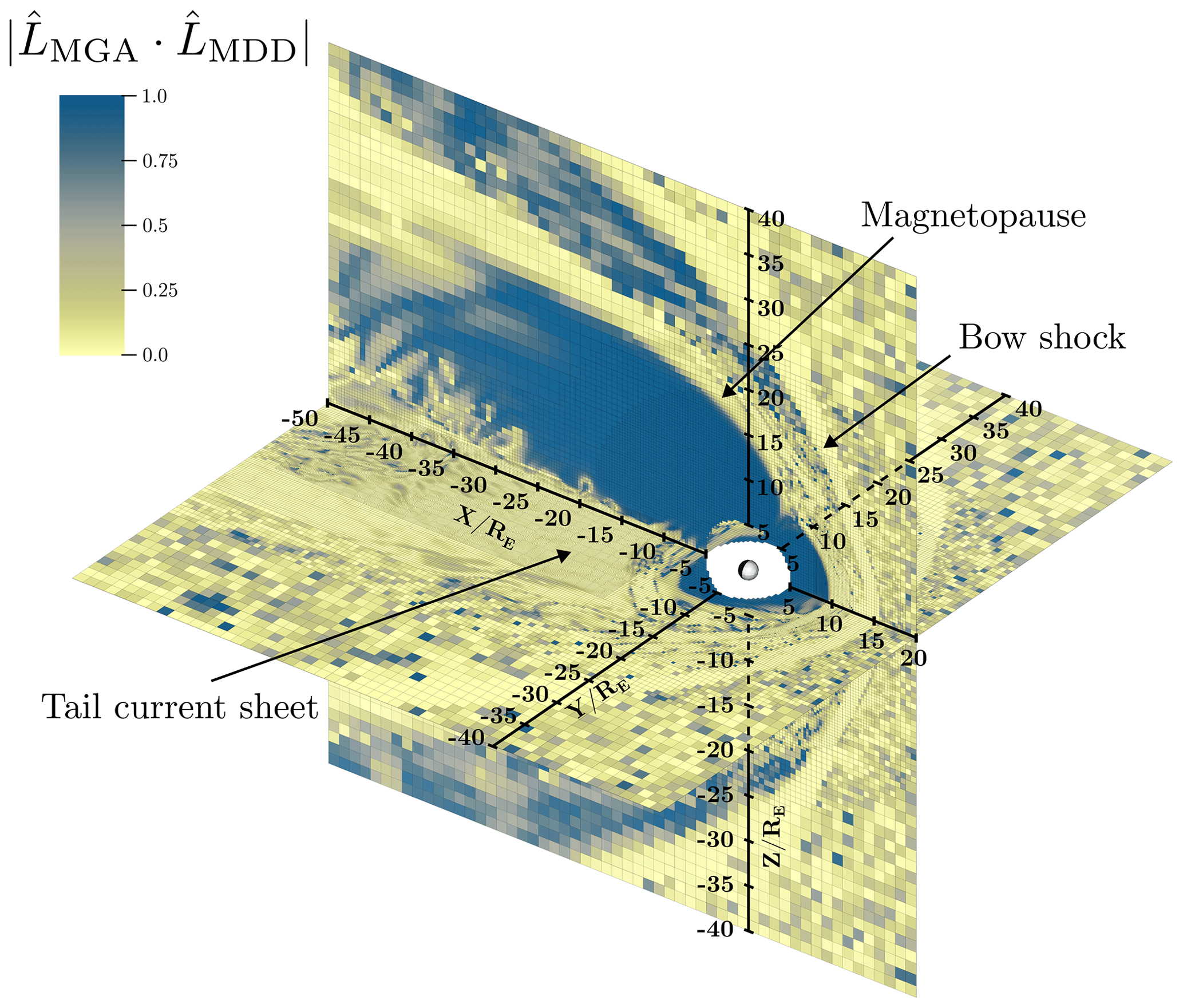
Figure 4Absolute value of the dot products of the primary and secondary vectors $| {\hat{L}}_{MGA} \cdot {\hat{L}}_{MDD} |$ used in the construction of the LMN systems, shown on the planes Y=0 and Z=0. We note that the vectors are nearly orthogonal, especially in the vicinity of the magnetopause and the tail current sheet, where we wish to employ the orthogonalized coordinate system.

Download

The sign of $\hat{L}$ and $\hat{N}$ in the global coordinates remains unfixed: multiplying both $\hat{L}$ and $\hat{N}$ by −1 does not affect the generality of the system. For now, this is left to be defined depending on the specific application.

Figure 4 shows the global magnetosphere as reproduced by the Vlasiator simulation, with Earth at the origin, the Sun on the lower right (in the direction of the positive x axis), and Earth's dipole field aligned to have the North Pole on the positive z axis. The figure displays the absolute value of the dot product ${\hat{L}}_{MGA} \cdot {\hat{L}}_{MDD}$ , a measure of non-orthogonality for the primary and secondary vectors of our LMN coordinate system on the Y=0 and Z=0 planes. In regions such as the magnetopause (X≈10 R_E at the subsolar point) and the bow shock (X≈15 R_E), hosting boundaries and CSs that are expected to be 1D structures, we see that the non-orthogonality is low. The magnetotail lobes and parts of the magnetosheath display consistent alignment of the primary and secondary vectors, indicating that the most-varying component of B varies most in the same direction, e.g. when approaching the polar regions along the magnetic field. This shows that care must be taken when considering these LMN coordinates, especially in the lobes and inner magnetosphere. The transition between the CS and the lobes in particular displays a complex structure.

While the above local coordinate system is defined where there is some variation in B, such that $| {\hat{L}}_{MGA} \cdot {\hat{L}}_{MDD} | < 1$ , and a non-zero electric current density J, our interest lies in reconnection-supporting CS structures, which naturally fulfil these conditions.

2.2 Contouring method

2.2.1 Finding reconnection-supporting CSs

In Palmroth et al. (2023), the CS centre was defined by the zero-crossing of the Earth-centred radial magnetic field component, B_r=0. This selects the crossover plane between the northern and southern lobes in the tail, with B_r=0 accounting for some radial component closer to the flanks. B_x=0 gives similar results in this case.

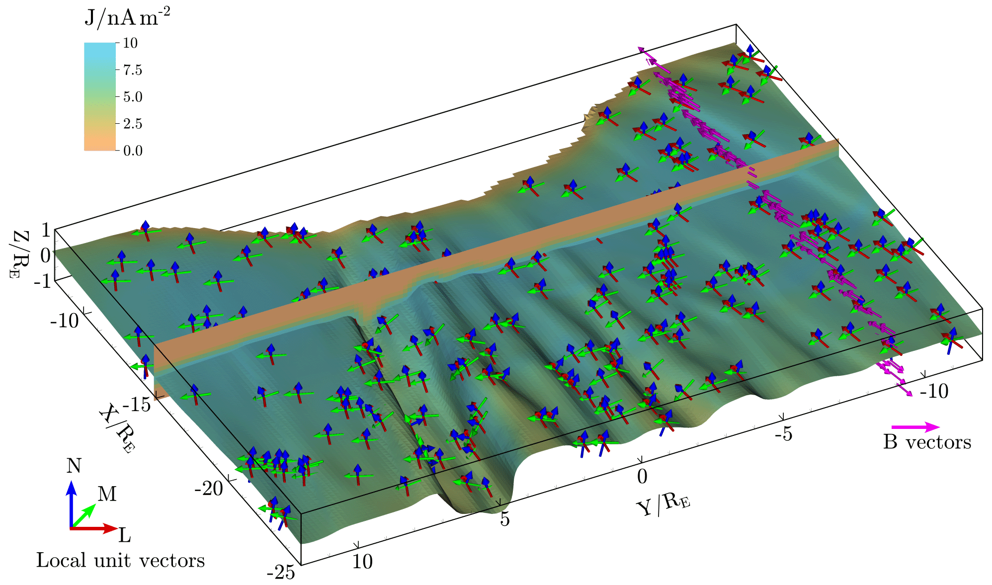
https://angeo.copernicus.org/articles/42/145/2024/angeo-42-145-2024-f05

Figure 5A Vlasiator tail CS (t = 1267 s). The CS centre plane is located by a contouring algorithm for B_L=0, forming a wavy sheet, which is coloured by the current density $| J |$ . For reference, the current density is also shown on the $X = - 15 R_{E}$ plane, indicating a match with the actual location of the CS. The local LMN basis vectors are shown on the CS (red: $\hat{L}$ , green: $\hat{M}$ , blue: $\hat{N}$ ) at arbitrary locations, and the B vectors are shown above and below the CS on a $Y = - 9 R_{E}$ slice (magenta).

Download

The local coordinate system, as given above, allows us to define an LMN system at each spatial cell of the simulation, analogously to the definition at each time in a time series for spacecraft observations. Finding B_L=0 surfaces shows the centres of symmetric CSs where the locally most-varying component of B changes its sign. While such a definition for the centre of a general current sheet is not strictly correct, it is sufficient for our purposes. These B_L=0 surfaces we deem to be the most interesting on the basis of supporting reconnection. However, with contouring algorithms, regions of consistent orientation of the LMN system need to be selected. As an example, the LMN coordinates of a Vlasiator tail CS, as shown in Fig. 5, have been homogenized by requiring $\hat{L} \cdot \hat{x} > 0$ and have been focused onto the CS by requiring $| J |$ > 2 nA m⁻². Figure 5 demonstrates, firstly, correct extraction of the CS midplane and, secondly, details of the local LMN basis vectors: the $\hat{L}$ vector tracks the orientation of the lobe fields, the $\hat{N}$ vector tracks the CS normal, and the $\hat{M}$ vector is in-plane and pointing in the general direction of the current.

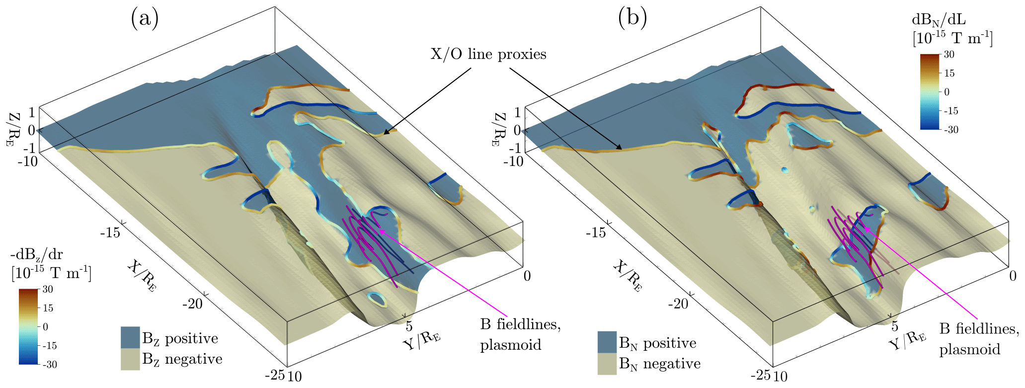
https://angeo.copernicus.org/articles/42/145/2024/angeo-42-145-2024-f06

Figure 6(a) Null lines obtained from B_r=0 and B_z=0 on the Vlasiator tail CS – local zoom-in of the simulation within the domain presented in Fig. 5. (b) LMN-contoured null lines. Both sheets are coloured by positive or negative B_z or B_N, respectively, with the null lines coloured by $- \partial_{r} B_{z}$ and ∂_LB_N, respectively. The strong CS flapping leads the former to miss a plasmoid on the flap, as shown by the field lines (magenta).

Download

2.2.2 Null lines

In Palmroth et al. (2023), the CS centre proxy B_r=0 serves as a basis for finding null lines on the sheet via the additional constraint of B_z=0. An example of these proxies and the flapping of the CS is shown in Fig. 6a. The sign of B_z serves as a proxy for field topology (given as sheet colour). We note that strong flapping of the CS causes the CS normal component to deviate strongly from the Z direction at points. Using the LMN basis allows us to take into consideration the local behaviour of the CS, improving upon the proxy model.

Finding the surfaces with B_L=0 and further intersecting those with the surfaces of B_N=0 yields a set of connected lines, as shown in Fig. 6b. For example, the contouring operator used by VisIt (Childs et al., 2012) finds these lines with topological connectivity. The left-hand side panel of Fig. 6 shows an example of the $B_{r} = B_{z} = 0$ contouring missing a plasmoid at a prominent CS flap, whereas the LMN method correctly finds the axis of the plasmoid. We note that the overall structure of the tail X and O lines is still well-described by the previous method outside of the region with large-amplitude flapping.

Above, and in general, we assume the existence of the normal component B_N for the detection of in-plane nulls. The potential degenerate case with B_N=0 over the entire CS (a tangential discontinuity) is hardly encountered in practice.

To use the LMN coordinate system and the components of magnetic field $B_{L}, B_{M}, B_{N}$ for contouring requires the LMN coordinate systems to be consistently oriented: if the ambiguity in the sign of L and N coordinates happens to flip between neighbouring cells, the B_L and B_N components will naturally change signs as well, as illustrated in Fig. 7. This is a source of false detections, which can be fixed by re-orienting neighbouring coordinate systems. In the magnetotail, for example, the choice we make is for L to point sunward so that, if the constructed LMN system has an initially tailward L, we multiply the L and N vectors by −1 in these cells. Automatic determination of consistently oriented neighbourhood charts could be considered in a future update. However, it may not be possible to provide a consistent orientation for the LMN coordinates in an entire domain, such as a global magnetospheric simulation. As long as there is a consistent orientation, the simple contouring operation works for current-sheet-like structures and produces topologically connected neutral lines.

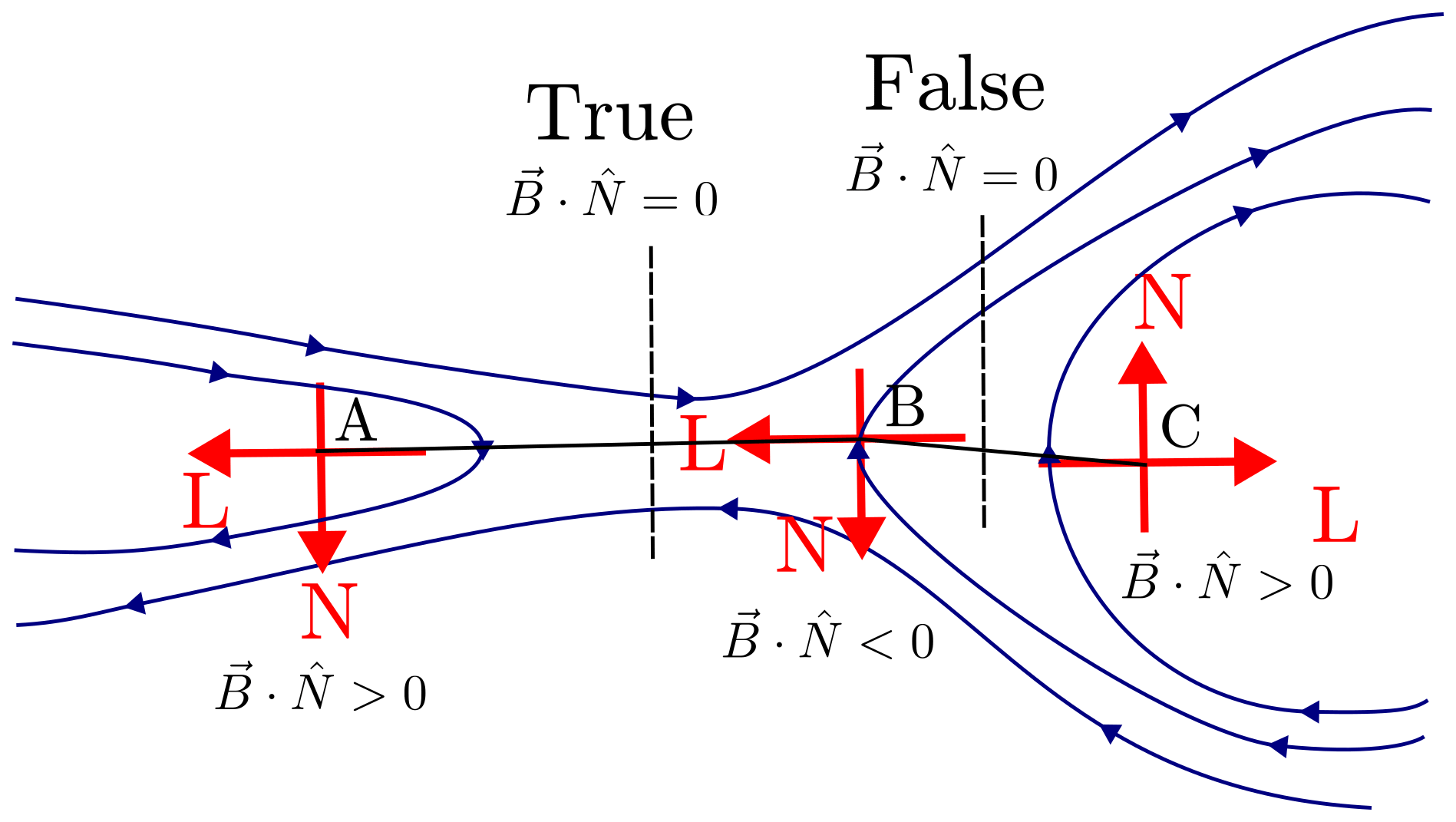
https://angeo.copernicus.org/articles/42/145/2024/angeo-42-145-2024-f07

Figure 7Schema of LN sign ambiguity and its effect. The signs of L and N vectors are not fixed by the construction and may vary arbitrarily. On the left is a correct evaluation of a B_N=0 (vertical dashed line) value between two points A and B, while on the right there is an incorrect evaluation of a B_N=0 value (vertical dashed line) between points B and C. The LN directions are locally correct but not necessarily consistent between neighbouring cells.

Download

When there is no consistent orientation available, naïve contouring does not work in an off-the-shelf manner. For example, in the case of the upstream solar wind, where Vlasiator shows very little variation in IMF, the LMN coordinate system is dominated by numerical precision artefacts, leading to inconsistent orientation showing up as noise in these contouring methods.

2.3 Cell-wise FOTE method

An alternative that does not require choices on orientation is to use the local data of B and G to construct first the local coordinate system and secondly a linear expansion of the components B_L and B_N at the cell centre. This sidesteps the ambiguity in the sign of the LN directions. Solving for the planes of B_L=0 and B_N=0 and their intersection is then straightforward in this linear approximation: $B_{L} + \nabla B_{L} \cdot r = 0$ is solved via an exact, single-step gradient descent along the negative gradient:

\begin{matrix} (5) & r = - \frac{B_{L}}{| \nabla B_{L} |} \cdot {\hat{e}}_{\nabla B_{L}}, \end{matrix}

where ${\hat{e}}_{\nabla B_{L}}$ is the unit vector in the direction of the gradient. This defines the plane B_L=0 with the normal direction ${\hat{e}}_{\nabla B_{L}}$ and a point r relative to the cell centre. Similarly, we find B_N=0 and the intersection line of these two planes.

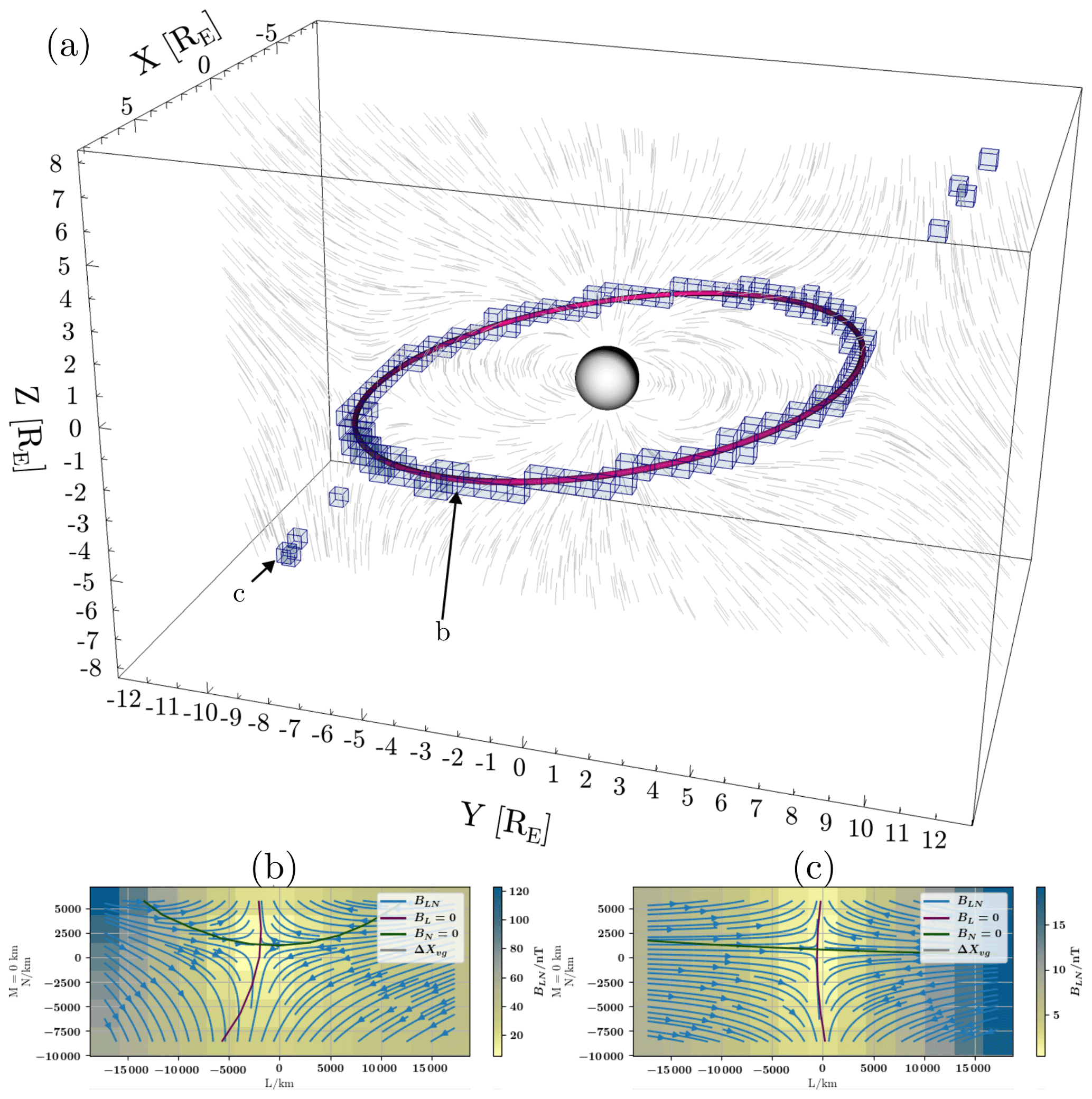
https://angeo.copernicus.org/articles/42/145/2024/angeo-42-145-2024-f08

Figure 8(a) Komar et al. (2013) 150° case reproduction: FOTE null lines (translucent blue cells) compared to analytical separator (magenta) and B field line stubs (light grey, from Y=0 plane) after slight propagation; note that the analytical separator is contained almost everywhere by the cells marked by the FOTE method. Bottom panels (b, c): LN slices at M=0 with magnetic field lines of in-plane components in blue, B_L=0 in black and B_N=0 in magenta. Background colour shows in-plane magnetic field magnitude. (b) This figure shows a detection of an X line in the vacuum superposition case (origin at cell marked by arrow b). (c) This figure shows an unexpected but correct detection of an X line in the vacuum superposition case (cell marked by arrow c).

Download

The line where $B_{L} = 0 = B_{N}$ would then again signify a null line, but the linear approximation can only be considered to be good within a small neighbourhood, that is, in the cell. It is then also straightforward to check whether or not this line intersects with the cell being analysed in the simulation coordinate system – if yes, we can consider the cell to contain a neutral line. We minimize a signed distance function (SDF; see e.g. Keinert et al., 2013) to the cell along the line, given by the definitions adapted from Korndörfer et al. (2015):

\begin{array}{l} (6) & d (r, b) & = {abs}^{e} (r) - b, \\ (7) & f_{box} (r, b) & = | | \max^{e} (d, 0) | | + \max (\min^{e} (d, 0)), \end{array}

where op^e denotes a component-wise operator (op) returning a vector of the same dimensionality, r is the query point, b is the upper corner of a rectangular cuboid centred at the origin and aligned with the coordinate system basis, and f_box is the SDF of the query point with respect to the cuboid. The SDF describes the distance of a point to the surface of an object, with positive values indicating that the point lies outside the object and negative values indicating that the point lies inside. Therefore, an SDF gives a continuous measure of the distance of the line with the cell, with negative values indicating the neutral line intersecting the cell and positive values indicating no intersection. This allows some evaluation and acceptance of near misses. A discriminating value of SDF≈0.25…0.36 is found to produce uninterrupted null lines in the tail, as expected based on field topology. Figure 8a shows examples of the FOTE method in use for Vlasiator data.

Further, we may evaluate the derivative ∂_LB_N at the cell and again classify the possible neutral line with it. Eigenvalues of G might as well be used for this purpose, as for degenerate nulls in Parnell et al. (1996), but we opt to use a straight derivative for a clear physical meaning. The main disadvantage for now is that this method does not provide a ready-made topology, only sets of cells that are considered to contain a segment of an X or O line.

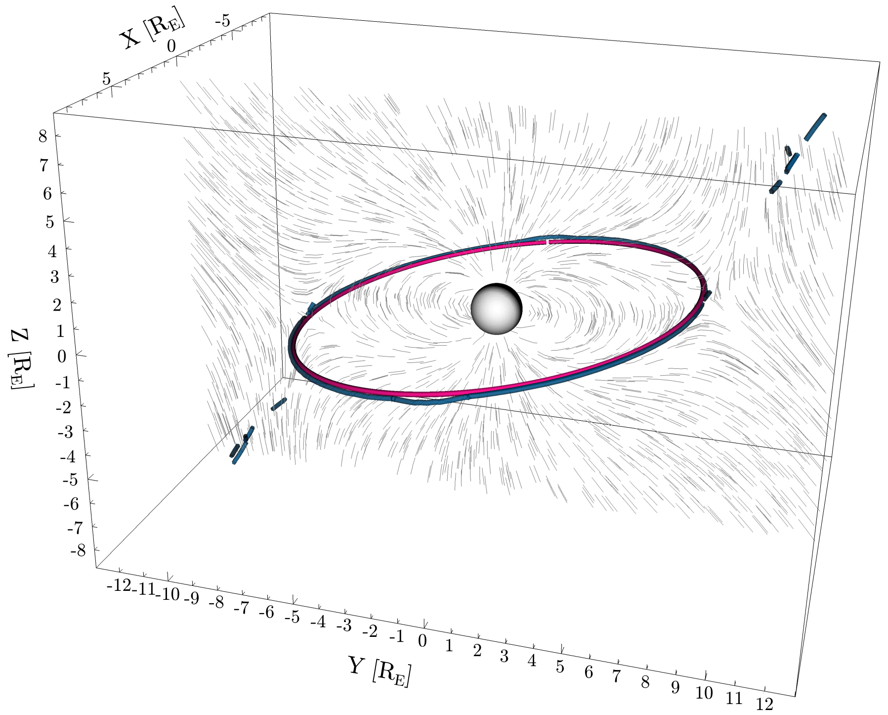
https://angeo.copernicus.org/articles/42/145/2024/angeo-42-145-2024-f09

Figure 9Komar et al. (2013) 150° case reproduction: contoured null lines (blue tubes) compared to analytical separator (magenta) and B field line stubs (light grey, from Y=0 plane) along the lines of Hu et al. (2009) and Komar et al. (2013) after slight propagation.

Download

3 Validation with an ideal case

We take the southward-IMF initial configurations of Hu et al. (2009) and Komar et al. (2013) for a test case that has null lines; the mentioned studies also provide analytical solutions for the magnetosphere using the methods by Yeh (1976). For the magnetic field configuration, we use as the constant IMF background magnetic field $B_{IMF} = (0, 32.5, - 56.3)$ nT for a field strength of 65 nT at a 150° clock angle and an unscaled terrestrial dipole aligned with the z axis. The domain size is $(\pm 2 \times 10^{5} km)^{3}$ , and the maximum spatial resolution is 3125 km. The current-free initial condition is not suitable to apply our method to since we use the current density vector to define the handedness of our coordinate basis. However, we choose to propagate the initial condition for a small time for the global plasma dynamics (7.048 ms). The background plasma is initialized at a density of 1 cm⁻³ as a radial taper of temperature and velocity from the inner boundary values of 5 MK and zero velocity to the solar wind values of 0.5 MK and 750 km s⁻¹ to break the exact current-free condition. This enables the use of our methods to extract the X line in the case with IMF clock angle θ = 150° (mostly southward IMF). To guard against current-free edge cases, we can use, as a fall-back case, the MGA maximum and medium variance coordinates for L and N directions instead.

Figure 8a shows a comparison between the FOTE method and the analytical solution. The cells detected by the FOTE method enclose the analytical separator nearly everywhere, but they show, in addition, a few extra null line segments further away. Figure 8b and c show details of the X-line detection by plotting L–N cross sections of the in-plane nulls. The origins of these cross sections are placed in the cells with FOTE-detected in-plane nulls, with the cross sections taken at M=0. The LMN basis is the local basis from the detection cell, extrapolated to the immediate neighbourhood. The slices show projections of the magnetic field lines in the LN plane and zero-crossing lines for B_N and B_L. The cross sections confirm these cells do contain in-plane null lines, as per our definition, but these are not described by the analytical solution for the separator. Figure 8 shows that these are indeed valid detections with an X topology. Notably, these detections are not present when inspecting the initial state with an MGA-only coordinate system and are likely a result of the initial velocity and temperature gradients causing minor perturbations.

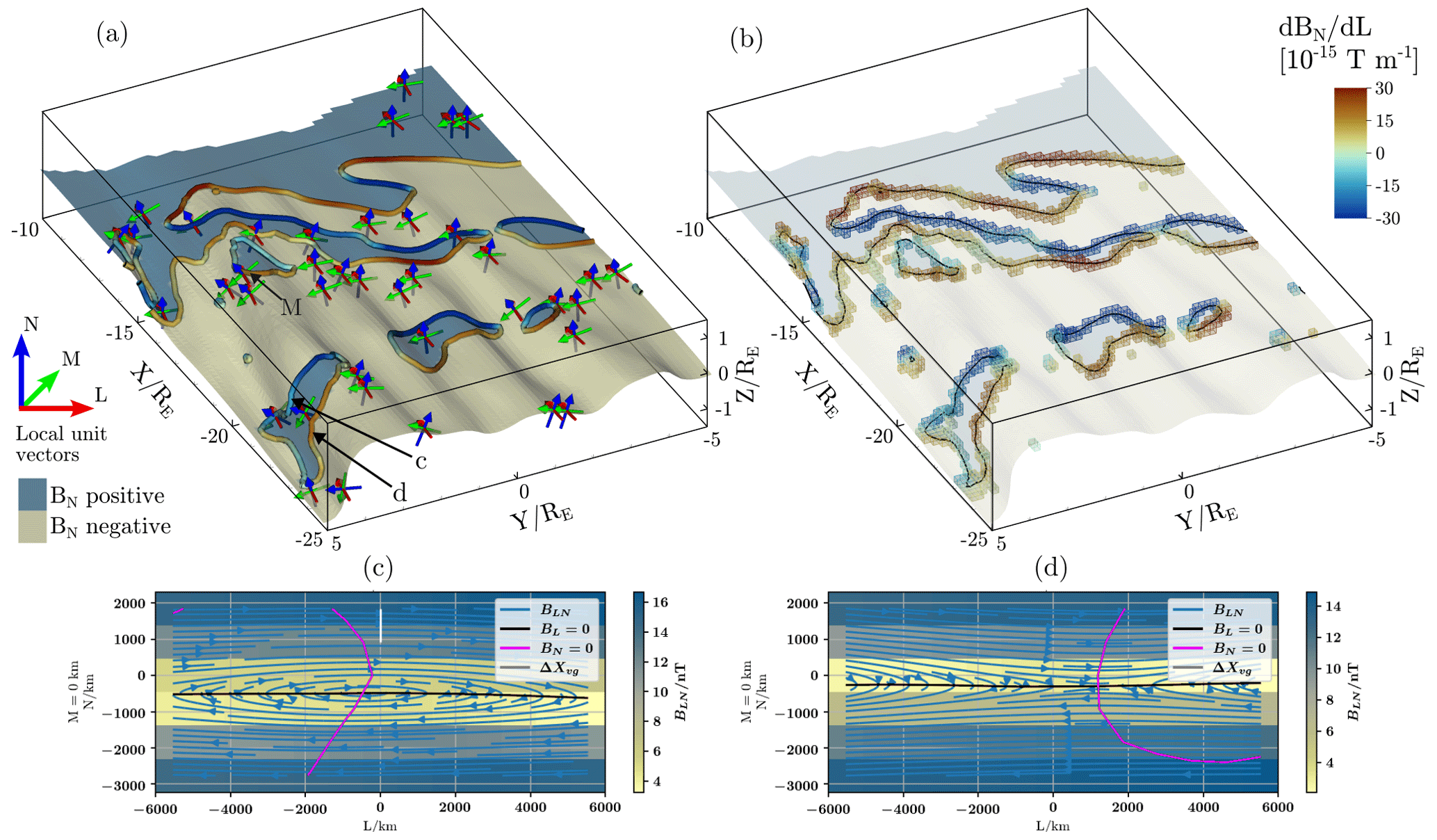
https://angeo.copernicus.org/articles/42/145/2024/angeo-42-145-2024-f10

Figure 10(a) The tail CS from Vlasiator simulation (EGI, t = 1267 s). Similar format to Fig. 6 LMN plot, with contoured X and O lines. (b) FOTE detections of X and O topologies (outlined cubic cells) compared with the contoured detections of panel (a) (black curves). Panels (c) and (d) show details from points marked by c and d, specifically a slice of the local L–N plane with in-plane magnetic field lines from streamline plotting of the in-plane magnetic field components and with zero contours of these components being annotated. The slices show that point c is correctly identified as an O topology, and point d is correctly identified as an X topology. The background colour is the strength of the in-plane magnetic field.

Download

Figure 9 shows a comparison between the contouring method and the analytical solution. Here, the LMN coordinate system has been regularized so that the L direction is chosen to fulfil $\hat{L} \cdot \hat{z} > 0$ . For this particular case, the LMN contouring of the superposition field produces prominent conical artefacts (not shown) where the coordinate system is not oriented consistently with this particular choice, and the data to be contoured are filtered to lie within one cell of a FOTE null line as a way to choose compact neighbourhoods of regularized orientation. Less stringent filtering can be used for other, more local cases (see, e.g. Sect. 4.1). Good agreement with the analytical solution is also seen in this case.

4 Results in Vlasiator

4.1 CS null lines in detail

Figure 10a and b show a section of the Vlasiator tail CS (a subset of Fig. 5). Firstly, panel (a) shows the in-plane null lines as found by the contouring method, coloured with ∂_LB_N (with red colours signifying X topologies and blue lines signifying O topologies). Evidently, the method struggles at the site of strong current sheet flapping. The CS is coloured by B_N, positive values are coloured blue, and negative values are coloured beige, extending the north–south classification in Fig. 6a to a flapping CS. The LMN coordinate bases are shown at some locations on the sheet as red–blue–green arrows. Further, two in-plane null line locations marked as (c) and (d) are chosen as examples (noting that these coincide with the flap seen in Fig. 6a), and for these locations the local LN plane magnetic field is plotted below in the corresponding panels (c) and (d), showing that these null lines are indeed correctly found and classified.

To validate the observed null lines with both methods in the case of the tail CS, Fig. 10b shows both contouring and FOTE detections at work, with the contoured in-plane null lines shown as black curves and the FOTE-detected null-line containing cells as wireframes coloured with ∂_LB_N. The methods agree well, even if the FOTE method may have some stray detections. These strays are found to be a minor issue, showing up on the current sheet as isolated cells flagged as containing null lines, while the true detections form coherent structures.

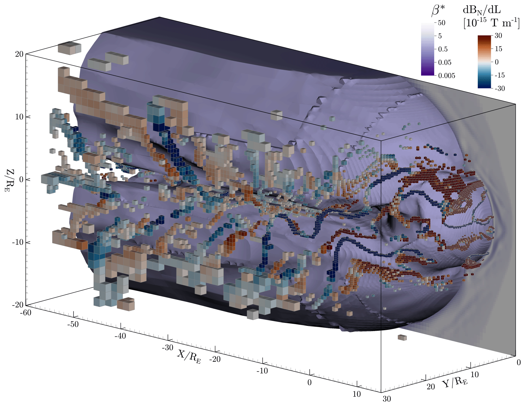
https://angeo.copernicus.org/articles/42/145/2024/angeo-42-145-2024-f11

Figure 11Dawn flank of the magnetosphere, with FOTE detections as outlined cells, using the β^∗ parameter on the vertical slice and on a magnetopause proxy at $β^{*} = 0.5$ .

Download

We may note that the local coordinate systems spanned by our LMN basis describe well the in-plane X and O lines in the simulation. However, this leads to the observation that the X and O line axes might not be aligned with the $\hat{M}$ direction, as also observed by Pathak et al. (2022) with MMS data. Figure 10 demonstrates this in the Vlasiator tail CS, with X and O lines necessarily breaking their alignment from the $\hat{M}$ direction when forming into loops, for example at $X = - 17 R_{E}$ , Y=3 R_E. The effect of this misalignment on reconnection in Vlasiator simulations is an ongoing subject of study.

4.2 Null lines in global Vlasiator 6D magnetosphere

To extend our analysis to the global Vlasiator magnetosphere, we use the generic FOTE method that is not limited by construction of consistently oriented neighbourhoods. The FOTE method reveals a sinuous and alternating neutral line structure on the magnetopause flanks, shown in Fig. 11. The O lines are marked with blue cells signifying dayside FTEs extending onto the flanks as a part of the sinuous pattern. The figure uses a magnetopause proxy from the β^∗ parameter of Xu et al. (2016), defined as

\begin{matrix} (8) & β^{*} = \frac{P_{thermal} + P_{dynamic}}{P_{B}} . \end{matrix}

Regions with small values of $| \partial_{L} B_{N} |$ (grey) should be inspected for their validity, in general, as these signify low variability in the magnetic field. These regions may be susceptible to local, insignificant perturbations fulfilling the FOTE criterion. The alternating pattern on the magnetopause at X<20 still suggests that these are indeed real magnetic structures, with alternating positive and negative B_N regions. We note, however, that the behaviour of the magnetopause on the flank in the present simulation is not yet studied in detail, and the shown time state (1267 s) may still contain initialization artefacts deep in the tail.

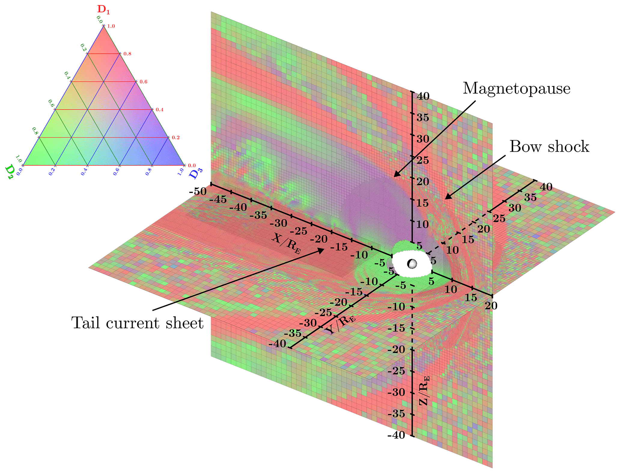
https://angeo.copernicus.org/articles/42/145/2024/angeo-42-145-2024-f12

Figure 12Overview of local MDD dimensionality, shown on the planes Y=0, Z=0. The dimensionality values $D = (D_{1}, D_{2}, D_{3}) \in [0, 1]^{3}$ are mapped to RGB colour channels via $rgb = D / 2 + (0.5, 0.5, 0.5)$ to obtain a three-channel representation of the triplet. See the ternary diagram at the top left for reference: the more red there is, the more 1D the local magnetic field structure is; green dominance signifies two-dimensionality, and blue dominance signifies three-dimensionality.

Download

4.3 Dimensionality of magnetic structures in Vlasiator

The applicability of the LMN coordinate system should be inspected in terms of dimensionality of the magnetic structures to ensure that the structures inspected are locally quasi-2D. Figure 12 shows an overview of the dimensionality measures D₁, D₂ and D₃ (Eqs. 2–4, described in Sect. 1.1) applied to a Vlasiator 6D simulation. Red colour corresponds to regions dominated by 1D variation (sheet-like structures), green corresponds to regions dominated by 2D structures (e.g. plasmoids and flux ropes), and blue corresponds to regions dominated by 3D structures. The upstream appears to be noisy as the magnetic field is nearly constant. The regions of interest for reconnection are naturally found in CSs, that is, mostly 1D structures with some embedded 2D features. These can be used to constrain the local basis analysis to compatible regions.

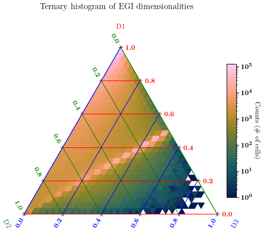
https://angeo.copernicus.org/articles/42/145/2024/angeo-42-145-2024-f13

Figure 13Local dimensionality of a Vlasiator simulation obtained via the MDD analysis; ternary histogram over most of the magnetosphere. Each cell outside of the inner boundary with r>5 R_E and constrained to −40 $R_{E} < X < 20 R_{E}$ and ± 40 R_E in Y and Z is shown here. The lack of completely 3D structures indicates that the in-plane approximation is usable.

Download

An interesting finding in the dimensionality parameters in the 6D Vlasiator run can be observed in the lack of dominantly 3D structures, as shown in Fig. 13. Magnetic structures exhibiting D₃ dominance appear to be limited: the occurrence of cells is increasingly rare as D₃→1. The prominent collection of cells having D₃=D₁ is found to be dominated by cells in the lobe regions of the magnetosphere. Whether or not these features are related to the divergence-free condition ∇⋅B, intrinsic properties of the magnetic field being convected by plasma, the boundary condition or other constraints remains to be studied.

5 Discussion and conclusions

Here, we have presented two local methods to acquire X and O topologies of the magnetic field from plasma simulations of Earth's magnetosphere, enabling fast and efficient identification of possible reconnection sites and flux transfer events. The algorithms work on O(N) complexity, i.e. operating once per grid cell (and possibly using a contouring algorithm of similar complexity) without requiring field line or separator tracing such as that used by Haynes and Parnell (2010). These methods use solely the magnetic field and its Jacobian, and so the found X lines may or may not be actively reconnecting – other methods need to be used to characterize the reconnection activity at the found sites, but the present methods have the advantage of being constrained to a local neighbourhood and only requiring knowledge about the magnetic field and its derivatives.

Using the dimensionality measures introduced by Rezeau et al. (2018) shows well that the magnetopause, the bow shock and the tail CS are essentially 1D structures, with intermittent, embedded 2D features. As we have a purely southward-IMF driving in the prototype case, this is consistent with Zeiler et al. (2002) observing that non-guide-field reconnection is mostly 2D. Future simulations including an IMF B_y component will provide stronger guide field reconnection and possibly different dimensionality of detected structures.

The construction of the local coordinate system involves some choices. The first in-plane direction $\hat{L}$ is given by the local MVA analogue (MGA). The normal direction $\hat{N}$ is chosen to be the primary eigenvector of the MDD system, orthogonalized with respect to $\hat{L}$ , to ensure good behaviour in nearly 1D CSs; the vector ∇B_L could be a conceivable option to supplant the secondary MDD vector, but this vector is not readily available from the magnetic field and its Jacobian.

For the contouring method, the limitation of requiring consistently oriented local coordinates is a slight issue. It could be mitigated by automated construction of local neighbourhood charts of consistent orientation, as well as automatically finding the extents where the local coordinate charts are sensible. As presented here, the contouring method relies on manual restriction of neighbourhoods for analysis. The FOTE method is given as a generalized alternative, operating cell-wise in the full domain, with the caveat that, in contrast to the contouring method, the FOTE method does not produce topological connectivity for the in-plane null lines; that is, it can be used to mark cells containing null lines but not which neighbouring cells those lines connect to. In contrast, the contouring method outputs line topologies from the isocontours of $B_{L} = 0 = B_{N}$ .

In comparison to topological methods, such as the magnetic skeleton method of Haynes and Parnell (2010), the present method does not require field line tracing or knowledge on boundary flows like the method proposed by Titov et al. (2009). On the other hand, Lapenta (2021) proposed a local Lorentz transformation method using both magnetic and electric fields, the latter of which the present method does not require. The present method can acquire useful null line objects via contouring, presenting something of a middle ground between local and topological analyses, adding another tool for studies of reconnection.

The presented FOTE and contouring methods are fundamental to investigate magnetic structures in a physically meaningful coordinate system, supporting reconnection studies in quasi-2D current sheets. The quantification of dimensionalities of magnetic structures may also provide new insights into plasma processes: for example, the magnetospheric tail lobes were found to be characterized by D₁≈D₃.

Code and data availability

Vlasiator is an open-source model, made available via Zenodo by Pfau-Kempf et al. (2022) (https://doi.org/10.5281/zenodo.3640593). A subset (the tail current sheet, ≈ 20 GB – a minimal data set for the reproduction of the Palmroth et al. (2023) study) of the Vlasiator run (totalling over 30 TB) used as the prototype case is publicly available as in Palmroth (2023). The open-source Analysator toolkit https://doi.org/10.5281/zenodo.4462514 (Battarbee et al., 2021) was employed for simulation data analysis.

Author contributions

MA, GC, IZ and FTK conceptualized the study, with MA, GC and IZ developing the methodology. MA wrote the original draft, implemented and applied the analysis tools, and performed validation and visualization. SH contributed to conceptualization and validation. UG, MB, YPK and KP developed and performed the relevant supercomputing simulation. JS and MA, along with UG, MB, YPK and KP, provided data curation. MP provided project administration, funding acquisition and supervision. All the authors reviewed the paper.

Competing interests

At least one of the (co-)authors is a member of the editorial board of Annales Geophysicae. The peer-review process was guided by an independent editor, and the authors also have no other competing interests to declare.

Disclaimer

Publisher's note: Copernicus Publications remains neutral with regard to jurisdictional claims made in the text, published maps, institutional affiliations, or any other geographical representation in this paper. While Copernicus Publications makes every effort to include appropriate place names, the final responsibility lies with the authors.

Acknowledgements

We acknowledge the European Research Council for the grants used to develop Vlasiator and PRACE for the supercomputing resources used for running the global simulations (see below for grant information). The authors wish to thank CSC – IT Center for Science in Finland, the Finnish Computing Competence Infrastructure (FCCI) and the University of Helsinki IT4SCI group for supporting this project with computational and data storage resources. The scientific colour maps by Crameri (2021) are used in this study to prevent visual distortion of the data and exclusion of readers with colour-vision deficiencies. The open-source VisIt visualization software (Childs et al., 2012) was used for data analysis and visualization. The authors thank Brian Walsh for the good questions, and thanks are also extended to Konstantinos Horaites for his comments.

Financial support

This research has been supported by the Research Council of Finland (grant nos. 336805, 328893, 335554, 322544, 339327, 339756 and 345701); the European Research Council, FP7 Ideas: European Research Council (grant no. 200141); the European Research Council, H2020 European Research Council (grant no. 682068); and the Partnership for Advanced Computing in Europe AISBL (grant no. 2019204998).

Open-access funding was provided by the Helsinki University Library.

Review statement

This paper was edited by Christopher Mouikis and reviewed by two anonymous referees.

References

Battarbee, M., Hannuksela, O. A., Pfau-Kempf, Y., Alfthan, S. V., Ganse, U., Jarvinen, R., Leo, Suni, J., Alho, M., Turc., L., Honkonen, I., Brito, T., and Grandin, M.: Fmihpc/Analysator: V0.9, Zenodo [code], https://doi.org/10.5281/zenodo.4462514, 2021. a

Bouri, I., Franssila, F., Alho, M., Cozzani, G., Zaitsev, I., Palmroth, M., and Roos, T.: Graph Representation of the Magnetic Field Topology in High-Fidelity Plasma Simulations for Machine Learning Applications, ICML 2023 Workshop on Machine Learning for Astrophysics, Honolulu, Hawaii, USA, https://doi.org/10.48550/arXiv.2307.09469, 2023. a

Bujack, R., Tsai, K., Morley, S. K., and Bresciani, E.: Open Source Vector Field Topology, SoftwareX, 15, 100787, https://doi.org/10.1016/j.softx.2021.100787, 2021. a

Bussov, M. and Nättilä, J.: Segmentation of Turbulent Computational Fluid Dynamics Simulations with Unsupervised Ensemble Learning, Signal Processing: Image Communication, 99, 116450, https://doi.org/10.1016/j.image.2021.116450, 2021. a

Childs, H., Brugger, E., Whitlock, B., Meredith, J., Ahern, S., Pugmire, D., Biagas, K., Miller, M., Harrison, C., Weber, G. H., Krishnan, H., Fogal, T., Sanderson, A., Garth, C., Bethel, E. W., Camp, D., Rübel, O., Durant, M., Favre, J. M., and Navrátil, P.: VisIt: An End-User Tool For Visualizing and Analyzing Very Large Data, in: High Performance Visualization–Enabling Extreme-Scale Scientific Insight, Chapman and Hall/CRC, New York, https://doi.org/10.1201/b12985, pp. 357–372, 2012. a, b

Crameri, F.: Scientific Colour Maps, Zenodo, https://doi.org/10.5281/ZENODO.1243862, 2021. a

Denton, R. E., Sonnerup, B. U. Ö., Birn, J., Teh, W.-L., Drake, J. F., Swisdak, M., Hesse, M., and Baumjohann, W.: Test of Methods to Infer the Magnetic Reconnection Geometry from Spacecraft Data, J. Geophys. Res.-Space, 115, A10242, https://doi.org/10.1029/2010JA015420, 2010. a, b

Dorelli, J. C. and Bhattacharjee, A.: On the Generation and Topology of Flux Transfer Events, J. Geophys. Res.-Space, 114, A06213, https://doi.org/10.1029/2008JA013410, 2009. a

Eggington, J. W. B., Desai, R. T., Mejnertsen, L., Chittenden, J. P., and Eastwood, J. P.: Time-Varying Magnetopause Reconnection During Sudden Commencement: Global MHD Simulations, J. Geophys. Res.-Space, 127, e2021JA030006, https://doi.org/10.1029/2021JA030006, 2022. a

Fu, H. S., Vaivads, A., Khotyaintsev, Y. V., Olshevsky, V., André, M., Cao, J. B., Huang, S. Y., Retinò, A., and Lapenta, G.: How to Find Magnetic Nulls and Reconstruct Field Topology with MMS Data?, J. Geophys. Res.-Space, 120, 3758–3782, https://doi.org/10.1002/2015JA021082, 2015. a

Ganse, U., Koskela, T., Battarbee, M., Pfau-Kempf, Y., Papadakis, K., Alho, M., Bussov, M., Cozzani, G., Dubart, M., George, H., Gordeev, E., Grandin, M., Horaites, K., Suni, J., Tarvus, V., Kebede, F. T., Turc, L., Zhou, H., and Palmroth, M.: Enabling Technology for Global 3D + 3V Hybrid-Vlasov Simulations of near-Earth Space, Phys. Plasmas, 30, 042902, https://doi.org/10.1063/5.0134387, 2023. a

Genestreti, K. J., Nakamura, T. K. M., Nakamura, R., Denton, R. E., Torbert, R. B., Burch, J. L., Plaschke, F., Fuselier, S. A., Ergun, R. E., Giles, B. L., and Russell, C. T.: How Accurately Can We Measure the Reconnection Rate EM for the MMS Diffusion Region Event of 11 July 2017?, J. Geophys. Res.-Space, 123, 9130–9149, https://doi.org/10.1029/2018JA025711, 2018. a, b

Glocer, A., Dorelli, J., Toth, G., Komar, C. M., and Cassak, P. A.: Separator Reconnection at the Magnetopause for Predominantly Northward and Southward IMF: Techniques and Results, J. Geophys. Res.-Space, 121, 140–156, https://doi.org/10.1002/2015JA021417, 2016. a

Gosling, J. T. and Phan, T. D.: MAGNETIC RECONNECTION IN THE SOLAR WIND AT CURRENT SHEETS ASSOCIATED WITH EXTREMELY SMALL FIELD SHEAR ANGLES, Astrophys. J., 763, L39, https://doi.org/10.1088/2041-8205/763/2/L39, 2013. a

Grandin, M., Luttikhuis, T., Battarbee, M., Cozzani, G., Zhou, H., Turc, L., Pfau-Kempf, Y., George, H., Horaites, K., Gordeev, E., Ganse, U., Papadakis, K., Alho, M., Tesema, F., Suni, J., Dubart, M., Tarvus, V., and Palmroth, M.: First 3D Hybrid-Vlasov Global Simulation of Auroral Proton Precipitation and Comparison with Satellite Observations, J. Space Weather Spac., 13, 20, https://doi.org/10.1051/swsc/2023017, 2023. a

Greene, J. M.: Geometrical Properties of Three-Dimensional Reconnecting Magnetic Fields with Nulls, J. Geophys. Res., 93, 8583, https://doi.org/10.1029/JA093iA08p08583, 1988. a

Harris, E. G.: On a Plasma Sheath Separating Regions of Oppositely Directed Magnetic Field, Nuovo Cimento (1955–1965), 23, 115–121, https://doi.org/10.1007/BF02733547, 1962. a

Haynes, A. L. and Parnell, C. E.: A Trilinear Method for Finding Null Points in a Three-Dimensional Vector Space, Phys. Plasmas, 14, 082107, https://doi.org/10.1063/1.2756751, 2007. a

Haynes, A. L. and Parnell, C. E.: A Method for Finding Three-Dimensional Magnetic Skeletons, Phys. Plasmas, 17, 092903, https://doi.org/10.1063/1.3467499, 2010. a, b, c

Hietala, H., Phan, T. D., Angelopoulos, V., Oieroset, M., Archer, M. O., Karlsson, T., and Plaschke, F.: In Situ Observations of a Magnetosheath High-Speed Jet Triggering Magnetopause Reconnection, Geophys. Res. Lett., 45, 1732–1740, https://doi.org/10.1002/2017GL076525, 2018. a

Hoilijoki, S., Ganse, U., Pfau-Kempf, Y., Cassak, P. A., Walsh, B. M., Hietala, H., von Alfthan, S., and Palmroth, M.: Reconnection Rates and X Line Motion at the Magnetopause: Global 2D-3V Hybrid-Vlasov Simulation Results, J. Geophys. Res.-Space, 122, 2877–2888, https://doi.org/10.1002/2016ja023709, 2017. a, b

Hoilijoki, S., Ganse, U., Sibeck, D. G., Cassak, P. A., Turc, L., Battarbee, M., Fear, R. C., Blanco-Cano, X., Dimmock, A. P., Kilpua, E. K. J., Jarvinen, R., Juusola, L., Pfau-Kempf, Y., and Palmroth, M.: Properties of Magnetic Reconnection and FTEs on the Dayside Magnetopause With and Without Positive IMF Bx Component During Southward IMF, J. Geophys. Res.-Space, 124, 4037–4048, https://doi.org/10.1029/2019JA026821, 2019. a

Horaites, K., Rintamäki, E., Zaitsev, I., Turc, L., Grandin, M., Cozzani, G., Zhou, H., Alho, M., Suni, J., Kebede, F., Gordeev, E., George, H., Battarbee, M., Bussov, M., Dubart, M., Ganse, U., Papadakis, K., Pfau-Kempf, Y., Tarvus, V., and Palmroth, M.: Magnetospheric Response to a Pressure Pulse in a Three-Dimensional Hybrid-Vlasov Simulation, J. Geophys. Res.-Space, 128, e2023JA031374, https://doi.org/10.1029/2023JA031374, 2023. a, b

Hu, Y. Q., Peng, Z., Wang, C., and Kan, J. R.: Magnetic Merging Line and Reconnection Voltage versus IMF Clock Angle: Results from Global MHD Simulations, J. Geophys. Res.-Space, 114, A08220, https://doi.org/10.1029/2009JA014118, 2009. a, b

Keinert, B., Schäfer, H., Korndörfer, J., Ganse, U., and Stamminger, M.: Improved Ray Casting of Procedural Distance Bounds, Journal of Graphics Tools, 17, 127–138, https://doi.org/10.1080/2165347X.2015.1033069, 2013. a

Komar, C. M., Cassak, P. A., Dorelli, J. C., Glocer, A., and Kuznetsova, M. M.: Tracing Magnetic Separators and Their Dependence on IMF Clock Angle in Global Magnetospheric Simulations, J. Geophys. Res.-Space, 118, 4998–5007, https://doi.org/10.1002/jgra.50479, 2013. a, b, c, d, e

Korndörfer, J. and Keinert, B., Ganse, U., Sänger, M., Ley, S., Burkhardt, K., Spuler, M., and Heusipp, J.: HG_SDF: A glsl library for building signed distance functions, Mercury Demogroup, https://mercury.sexy/hg_sdf (last access: 25 April 2023), 2015. a

Laitinen, T. V., Janhunen, P., Pulkkinen, T. I., Palmroth, M., and Koskinen, H. E. J.: On the characterization of magnetic reconnection in global MHD simulations, Ann. Geophys., 24, 3059–3069, https://doi.org/10.5194/angeo-24-3059-2006, 2006. a, b, c

Lapenta, G.: Detecting Reconnection Sites Using the Lorentz Transformations for Electromagnetic Fields, Astrophys. J., 911, 147, https://doi.org/10.3847/1538-4357/abeb74, 2021. a

Lau, Y.-T. and Finn, J. M.: Three-Dimensional Kinematic Reconnection in the Presence of Field Nulls and Closed Field Lines, Astrophys. J., 350, 672, https://doi.org/10.1086/168419, 1990. a

Olshevsky, V., Divin, A., Eriksson, E., Markidis, S., and Lapenta, G.: ENERGY DISSIPATION IN MAGNETIC NULL POINTS AT KINETIC SCALES, Astrophys. J., 807, 155, https://doi.org/10.1088/0004-637X/807/2/155, 2015. a

Olshevsky, V., Deca, J., Divin, A., Peng, I. B., Markidis, S., Innocenti, M. E., Cazzola, E., and Lapenta, G.: MAGNETIC NULL POINTS IN KINETIC SIMULATIONS OF SPACE PLASMAS, Astrophys. J., 819, 52, https://doi.org/10.3847/0004-637X/819/1/52, 2016. a, b

Palmroth, M.: Vlasiator 6D 'EGI' Tail Current Sheet Data Series, University of Helsinki [data set], https://doi.org/10.23729/72EFF3EF-C84B-43B8-94D1-0A8B49C7C56D, 2023. a, b

Palmroth, M., Hoilijoki, S., Juusola, L., Pulkkinen, T. I., Hietala, H., Pfau-Kempf, Y., Ganse, U., von Alfthan, S., Vainio, R., and Hesse, M.: Tail reconnection in the global magnetospheric context: Vlasiator first results, Ann. Geophys., 35, 1269–1274, https://doi.org/10.5194/angeo-35-1269-2017, 2017. a, b

Palmroth, M., Ganse, U., Pfau-Kempf, Y., Battarbee, M., Turc, L., Brito, T., Grandin, M., Hoilijoki, S., Sandroos, A., and von Alfthan, S.: Vlasov Methods in Space Physics and Astrophysics, Living Reviews in Computational Astrophysics, 4, 1, https://doi.org/10.1007/s41115-018-0003-2, 2018. a

Palmroth, M., Pulkkinen, T. I., Ganse, U., Pfau-Kempf, Y., Koskela, T., Zaitsev, I., Alho, M., Cozzani, G., Turc, L., Battarbee, M., Dubart, M., George, H., Gordeev, E., Grandin, M., Horaites, K., Osmane, A., Papadakis, K., Suni, J., Tarvus, V., Zhou, H., and Nakamura, R.: Magnetotail Plasma Eruptions Driven by Magnetic Reconnection and Kinetic Instabilities, Nat. Geosci., 16, 570–576, https://doi.org/10.1038/s41561-023-01206-2, 2023. a, b, c, d, e, f, g, h, i, j

Parker, E. N.: Sweet's Mechanism for Merging Magnetic Fields in Conducting Fluids, J. Geophys. Res. (1896–1977), 62, 509–520, https://doi.org/10.1029/JZ062i004p00509, 1957. a

Parnell, C. E., Smith, J. M., Neukirch, T., and Priest, E. R.: The Structure of Three-dimensional Magnetic Neutral Points, Phys. Plasmas, 3, 759–770, https://doi.org/10.1063/1.871810, 1996. a

Parnell, C. E., Haynes, A. L., and Galsgaard, K.: Structure of Magnetic Separators and Separator Reconnection, J. Geophys. Res.-Space, 115, A02102, https://doi.org/10.1029/2009JA014557, 2010. a

Paschmann, G. and Daly, P. W.: Analysis Methods for Multi-Spacecraft Data, no. SR-001 in ISSI Scientific Report, ESA Publications Division, ESA Publications Division Keplerlaan 1, 2200 AG Noordwijk, the Netherlands, 1998. a

Pathak, N., Ergun, R. E., Qi, Y., Schwartz, S. J., Vo, T., Usanova, M. E., Hesse, M., Phan, T. D., Drake, J. F., Eriksson, S., Ahmadi, N., Chasapis, A., Wilder, F. D., Stawarz, J. E., Burch, J. L., Genestreti, K. J., Torbert, R. B., and Nakamura, R.: Evidence of a Nonorthogonal X-line in Guide-field Magnetic Reconnection, Astrophys. J. Letters, 941, L34, https://doi.org/10.3847/2041-8213/aca679, 2022. a

Pfau-Kempf, Y., Palmroth, M., Johlander, A., Turc, L., Alho, M., Battarbee, M., Dubart, M., Grandin, M., and Ganse, U.: Hybrid-Vlasov Modeling of Three-Dimensional Dayside Magnetopause Reconnection, Phys. Plasmas, 27, 092903, https://doi.org/10.1063/5.0020685, 2020. a, b

Pfau-Kempf, Y., von Alfthan, S., Ganse, U., Sandroos, A., Battarbee, M., Koskela, T., Otto, Ilja, Papadakis, K., Kotipalo, L., Zhou, H., Grandin, M., Pokhotelov, D., and Alho, M.: Fmihpc/Vlasiator: Vlasiator, Zenodo [code], https://doi.org/10.5281/zenodo.3640593, 2022. a

Priest, E. R. and Titov, V. S.: Magnetic Reconnection at Three-Dimensional Null Points, Philos. T. Roy. Soc. A, 354, 2951–2992, https://doi.org/10.1098/rsta.1996.0136, 1996. a

Rezeau, L., Belmont, G., Manuzzo, R., Aunai, N., and Dargent, J.: Analyzing the Magnetopause Internal Structure: New Possibilities Offered by MMS Tested in a Case Study, J. Geophys. Res.-Space, 123, 227–241, https://doi.org/10.1002/2017JA024526, 2018. a, b

Servidio, S., Matthaeus, W. H., Shay, M. A., Cassak, P. A., and Dmitruk, P.: Magnetic Reconnection in Two-Dimensional Magnetohydrodynamic Turbulence, Phys. Rev. Lett., 102, 115003, https://doi.org/10.1103/PhysRevLett.102.115003, 2009. a

Shen, C., Rong, Z. J., Li, X., Dunlop, M., Liu, Z. X., Malova, H. V., Lucek, E., and Carr, C.: Magnetic configurations of the tilted current sheets in magnetotail, Ann. Geophys., 26, 3525–3543, https://doi.org/10.5194/angeo-26-3525-2008, 2008. a

Shi, Q. Q., Tian, A. M., Bai, S. C., Hasegawa, H., Degeling, A. W., Pu, Z. Y., Dunlop, M., Guo, R. L., Yao, S. T., Zong, Q.-G., Wei, Y., Zhou, X.-Z., Fu, S. Y., and Liu, Z. Q.: Dimensionality, Coordinate System and Reference Frame for Analysis of In-Situ Space Plasma and Field Data, Space Sci. Rev., 215, 35, https://doi.org/10.1007/s11214-019-0601-2, 2019. a, b, c, d, e, f

Sonnerup, B. and Scheible, M.: Minimum and Maximum Variance Analysis, in: Analysis Methods for Multi-Spacecraft Data, vol. 001 of ISSI Scientific Report, International Space Science Institute, Bern, Switzerland, pp. 185–220, 1998. a

Sonnerup, B. U. Ö.: Magnetic-Field Re-Connexion in a Highly Conducting Incompressible Fluid, J. Plasma Phys., 4, 161–174, https://doi.org/10.1017/S0022377800004888, 1970. a

Sonnerup, B. U. Ö.: Magnetopause Reconnection Rate, J. Geophys. Res. (1896–1977), 79, 1546–1549, https://doi.org/10.1029/JA079i010p01546, 1974. a

Titov, V. S., Forbes, T. G., Priest, E. R., Mikić, Z., and Linker, J. A.: SLIP-SQUASHING FACTORS AS A MEASURE OF THREE-DIMENSIONAL MAGNETIC RECONNECTION, Astrophys. J., 693, 1029, https://doi.org/10.1088/0004-637X/693/1/1029, 2009. a

von Alfthan, S., Pokhotelov, D., Kempf, Y., Hoilijoki, S., Honkonen, I., Sandroos, A., and Palmroth, M.: Vlasiator: First Global Hybrid-Vlasov Simulations of Earth's Foreshock and Magnetosheath, J. Atmos. Sol.-Terr. Phy, 120, 24–35, https://doi.org/10.1016/j.jastp.2014.08.012, 2014. a

Xu, S., Liemohn, M. W., Dong, C., Mitchell, D. L., Bougher, S. W., and Ma, Y.: Pressure and Ion Composition Boundaries at Mars, J. Geophys. Res.-Space, 121, 6417–6429, https://doi.org/10.1002/2016JA022644, 2016. a

Yeates, A. R. and Hornig, G.: A Generalized Flux Function for Three-Dimensional Magnetic Reconnection, Phys. Plasmas, 18, 102118, https://doi.org/10.1063/1.3657424, 2011. a

Yeh, T.: Reconnection of Magnetic Field Lines in Viscous Conducting Fluids, J. Geophys. Res. (1896-1977), 81, 4524–4530, https://doi.org/10.1029/JA081i025p04524, 1976. a

Zeiler, A., Biskamp, D., Drake, J. F., Rogers, B. N., Shay, M. A., and Scholer, M.: Three-Dimensional Particle Simulations of Collisionless Magnetic Reconnection, J. Geophys. Res.-Space, 107, SMP 6-1–SMP 6-9, https://doi.org/10.1029/2001JA000287, 2002. a

Articles

Short summary

Magnetic reconnection is one of the main processes for energy conversion and plasma transport in space plasma physics, associated with plasma entry into the magnetosphere of Earth and Earth’s substorm cycle. Global modelling of these plasma processes enables us to understand the magnetospheric system in detail. However, finding sites of active reconnection from large simulation datasets can be challenging, and this paper develops tools to find magnetic topologies related to reconnection.