the Creative Commons Attribution 4.0 License.
the Creative Commons Attribution 4.0 License.
 | 13 Dec 2019
Generation of Rossby waves off the Cape Verde Peninsula: the role of the coastline
Jérôme Sirven
Juliette Mignot
Michel Crépon
In December 2002 and January 2003 satellite observations of chlorophyll showed a strong coastal signal along the west African coast between 10 and 22∘ N. In addition, a wavelike pattern with a wavelength of about 750 km was observed from 20 December 2002 and was detectable for 1 month in the open sea, south-west of the Cape Verde Peninsula. Such a pattern suggests the existence of a locally generated Rossby wave which slowly propagated westward during this period. This hypothesis was confirmed by analysing sea surface height provided by satellite altimeter during this period. To decipher the mechanisms at play, a numerical study based on a reduced-gravity shallow-water model has first been conducted. A wind burst, broadly extending over the region where the offshore oceanic signal is observed, is applied for 5 d. A Kelvin wave quickly develops along the northern edge of the cape, then propagates and leaves the area in a few days. Simultaneously, a Rossby wave whose characteristics seem similar to the observed pattern forms and slowly propagates westward. The existence of the peninsula limits the extent of the wave to the north. The spatial extent of the wind burst determines the extent of the response and correspondingly the timescale of the phenomenon (about 100 d in the present case). When the wind burst has a large zonal and small meridional extent, the behaviour of a wave to the north of the peninsula differs from that to the south. These results are corroborated and completed by an analytical study of a linear reduced-gravity model using a non-Cartesian coordinate system. This system is introduced to evaluate the potential impact of the coastline shape. The analytical computations confirm that a period of around 100 d can be associated with the observed wave considering the value of the wavelength; they also show that the role of the coastline remains moderate at such timescales. By contrast, when the period becomes shorter (smaller than 20–30 d), the behaviour of the waves is modified because of the shape of the coast. South of the peninsula, a narrow band of sea isolated from the rest of the ocean by two critical lines appears. Its meridional extent is about 100 km and Rossby waves could propagate there towards the coast.


Eastern boundary upwelling systems (EBUSs) – such as the California, Humboldt, Canary and Benguela upwelling systems – constitute a ubiquitous feature of the coastal ocean dynamics, which has been extensively studied. They are biologically very productive thanks to the transport of nutrients from deep ocean layers to the surface, which favours the bloom of phytoplankton. Consequently they present a strong signature, which is detectable by ocean colour satellite sensors (see, for example, Lachkar and Gruber, 2012, 2013).
The dynamics of EBUS were first studied with conceptual models. Upwellings are created by alongshore equatorward winds (Allen, 1976; McCreary et al., 1986) generating an offshore Ekman transport, which is compensated for by a vertical transport at the coast in order to satisfy the mass conservation. The near-shore pattern of the upwellings is affected by the baroclinic instability mechanism which is associated with the coastal current system and produces eddies and filaments (Marchesiello et al., 2003). Lastly wind fluctuations modulate the upwelling intensity by generating Kelvin waves propagating poleward (Moore, 1968; Allen, 1976; Gill and Clarke, 1974; Clarke, 1977; 1983; McCreary, 1981).
At a given frequency, there is a critical latitude poleward of which Kelvin waves no longer exist and are replaced by Rossby waves propagating westward (Schopf et al., 1981; Clarke, 1983; McCreary and Kundu, 1985). The critical latitude decreases when the wave period shortens (Grimshaw and Allen, 1988) or when the coastline angle with the poleward direction increases (Clarke and Shi, 1991). This latter property suggests that the shape of the coast has an impact on the upwellings.
Using a high-resolution 3-D numerical model, Batteen (1997) then Marchesiello et al. (2003) confirmed that the shape of the coastline actually plays a role in the upwelling pattern. However, they did not investigate by which mechanisms they are driven. In particular they did not try to compare their results with the theoretical investigations of Crépon and Richez (1982) and Crépon et al. (1984), who analysed the mechanisms responsible for this behaviour. Using an f-plane model, these authors showed that a cape modifies the characteristics of the upwelling, its intensity being less on the upwind side of the cape than on the downwind side. However, they did not investigate what occurs in the open sea up to 1000 km from the coast and which role the β effect could play.
The role of the forcing has also been investigated, both from observational and theoretical viewpoints. Enriquez and Friehe (1995) computed the wind stress and wind stress curl off the California shelf from aircraft measurements and, thanks to numerical experiments with a two-layer model and an analytical study, showed that a non-zero wind stress curl expands the horizontal extent of upwelling offshore; it increases from 20–30 to 80–100 km. The importance of the wind stress curl, which generates a strong Ekman pumping, was first emphasized by Richez et al. (1984). Later, Pickett and Paduan (2003) could establish that the Ekman pumping and the Ekman transport due to the alongshore winds have a comparable importance in the California Current area; Castelao and Barth (2006) found a similar result off Cabo Frio in Brazil. These contributions did not study what occurs beyond 100 km from the coast.
In the present paper, we study the role of wind stress and coastline geometry in generating mesoscale anomalies offshore, up to a distance of 500–1000 km off the coast. Both a numerical and an analytical point of view are adopted. The departure point is the observation of a wave-like pattern on chlorophyll satellite observations off the Senegalese coast, in the region of the Senegal–Mauritanian upwelling (see Lathuillière et al., 2008, and Farikou et al., 2015, for further information about the chl a variability and the upwellings off the west African coast, Capet et al., 2017, for a recent analysis of the small-scale variability close to the Senegal and Gambia coasts, and Kounta et al., 2018, for a detailed study of the slope currents along west Africa). Attention is focused on offshore mesoscale activity associated with the upwelling, a recurrent feature of upwelling systems (see Capet et al., 2008a, b). The alongshore activity, which has received much more attention (see, for example, Diakhaté et al., 2016, and the references therein) is not studied.
The paper is structured as follows. Observations of chlorophyll in 2002–2003 off the west African coast are shown and described in Sect. 2. In Sect. 3, a numerical study with a non-linear reduced-gravity shallow-water model on the sphere with a single active layer is conducted; it shows that a wind stress anomaly active for a few days can generate a pattern that seems very similar to the observed one. The impacts of the wind anomaly extent and coastline geometry are also briefly studied. In Sect. 4, a theoretical analysis of the wave dynamics in the vicinity of a cape is conducted to confirm and enlarge upon the results obtained in the previous section, using a linear shallow-water model in a non-Cartesian coordinate system.
The Senegal–Mauritanian upwelling off the west coast of Africa forms the southern part of the Canary upwelling system. This region has been intensively studied by analysis of SeaWiFS (Sea-viewing Wide Field-of-View Sensor) ocean colour data and AVHRR (Advanced Very High Resolution Radiometer) sea surface temperature as reported in Demarcq and Faure (2000) and more recently by Sawadogo et al. (2009), Farikou et al. (2013, 2015), Ndoye et al. (2014), and Capet et al. (2017). These studies indicate that the presence of an intense upwelling is attested by ocean colour and sea surface temperature signals. Moreover this upwelling shows a strong seasonal modulation. It starts to intensify in October, reaches its maximum in April and slows down in June. Very high chlorophyll a concentrations are observed near the coast where the maximum is reached. However, the concentration rapidly decreases offshore (Farikou et al., 2013, 2015; Sawadogo et al., 2009), suggesting that the upwelling extent and the eddy activity in this region are less than in other upwelling systems like the Californian upwelling system (Marchesiello and Estrade, 2009; Capet et al., 2017).
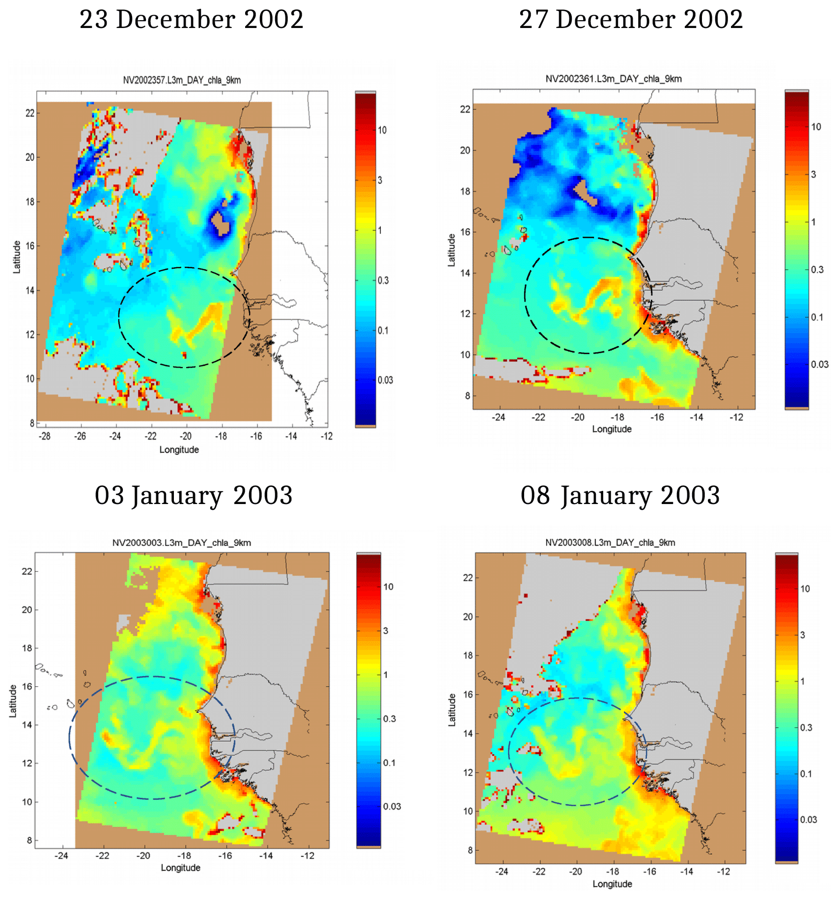
Figure 1Chlorophyll observed by SeaWiFS at 4 different days. A wave-like pattern (which is circled by a dashed line) is visible between −22 and in longitude and 12 and 14∘ in latitude. At the end of the period a westward propagation seems to initiate. The chlorophyll concentration is given in milligrams per cubic metre by the colour bar at the right of the maps.
From 20 December 2002 up to 8 January 2003, a strong chlorophyll signal was observed along the African coast on SeaWiFS satellite images, between 10 and 22∘ N, indicating intense biological activity. In addition, a well-defined “sine-like” pattern (circled in Fig. 1) was observed on 10 images taken on 10 non-consecutive days, which excludes a possible artefact due to image processing. This pattern is located between 12 and 14∘ N, east of 20∘ W, and extends offshore up to 22∘ W in a region which is off the coastal upwelling zone. West of 20∘ W the signal seems to have a larger meridional extent, reaching 16–17∘ N (see panel “03 January 2003”).
This pattern, which broadly keeps the same form during a 20 d interval, slowly progresses westward at a speed not exceeding 5 cm s−1 (a more precise estimation of the speed from the observations is quite risky). After 8 January 2003, a cloudy period of several days occurred, which prevented satellite observations. At the end of this episode (15 January) the sine pattern was no longer visible. This episode might be the signature of a Rossby wave propagating westward. As this phenomenon lasts at least 1 month, its typical timescale is expected to range between 1 and a few months.
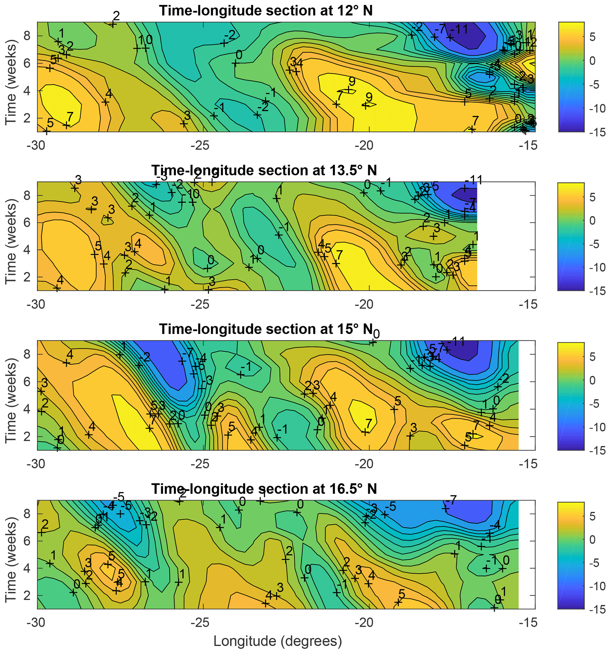
Figure 2Hovmöller diagrams of the SSH at latitudes 12, 13.5, 15, and 16.5∘ N (the SSH amplitude is given in centimetre by the colour bar at the right of the diagrams). Note the decrease in the amplitude at 16.5∘ N. The phase velocity of the wave is about 4.5 cm s−1.
To corroborate this hypothesis, we analysed the sea surface height (hereafter SSH) obtained from AVISO (Archiving, Validation and Interpretation of Satellite Oceanographic data) satellite altimeter data for the corresponding period (December 2002–January 2003). Hovmöller diagrams are shown at 12, 13.5, 15, and 16.5∘ in Fig. 2; they clearly confirm the existence of a Rossby wave propagating westwards with a velocity of about 4.5 cm s−1. The amplitude of this wave becomes smaller northwards: it peaked at 13 cm between 12 and 13.5∘ but did not exceed 7 cm at 16.5∘. The wavelength is around 700 km, comparable with the extent of the chlorophyll signal.
An enhanced chlorophyll concentration, as seen by the satellite sensor, is the signature of growing phytoplankton. A local development of phytoplankton benefits from an increase in the nutrient concentration in the surface layers of the ocean. The latter may be generated by an enhanced mixing in the surface layers associated with an increased turbulence due to the Kelvin or Rossby wave activity and by the vertical velocity associated with the divergent Rossby waves. Another possible process explaining this growth could be the advection linked with Rossby waves – they create a current anomaly which can transport nutrients and phytoplankton from the upwelling area where they are highly concentrated. However, this mechanism is slow; for a current anomaly of 5 cm s−1, the transport of a parcel of fluid over 500 km – less than the zonal extent of the offshore pattern – would need about 1 year.
The signal along the coast is also modulated by coastal Kelvin waves propagating northwards. Clarke and Shi (1991) showed that they can propagate when their angular frequency is larger than a critical angular frequency . In this formula Θ is an angle taking into account the tilt of the coastline with a meridian, c a typical velocity of a baroclinic mode, and f0 and β the usual parameters linked to the Earth's rotation. These authors found that ωc ranges between 84.69 and 115.2 d around the Cape Verde Peninsula (see their Table 2a). These values are close to the characteristic timescales we expect here.
The existence of a long period divergent baroclinic Rossby wave, evidenced by the AVISO satellite altimeter data of the SSH, can explain the offshore sine-like pattern described here. To investigate the mechanism of emergence of this wave and analyse its properties, we first describe numerical experiments made with a numerical shallow-water model. They help us see how such a wave is created and elucidate its nature. Then, a theoretical analysis is presented in order to understand how the Kelvin and Rossby waves behave when the coast presents a cape and to complete the interpretation of the numerical experiments. A wide range of periods is explored, going from 10 d to 1 year.
3.1 The model
The numerical model is a reduced-gravity model on the sphere with one active layer of thickness h. It extends over an infinite layer at rest. The velocity v in the active layer and the thickness h verify the equations
and
where n is a vector normal to the Earth's surface and . The function Φ is equal to where g⋆ is the reduced gravity.
We assume for simplicity that the vector τ0, which represents the surface wind stress divided by the ocean density, derives from a potential ϕ0(x,y): (implying an irrotational mean wind). This hypothesis allows us to compute explicitly the obtained mean state. Indeed, v=0 and are an obvious solution of the previous system (the constant C0 is determined by using the fact that the mean value of h0 remains unchanged during the integration). It will also facilitate the analytical computations made in the next section. A more complex set-up could be used for the numerical experiments, but it will be seen below that this one suffices.
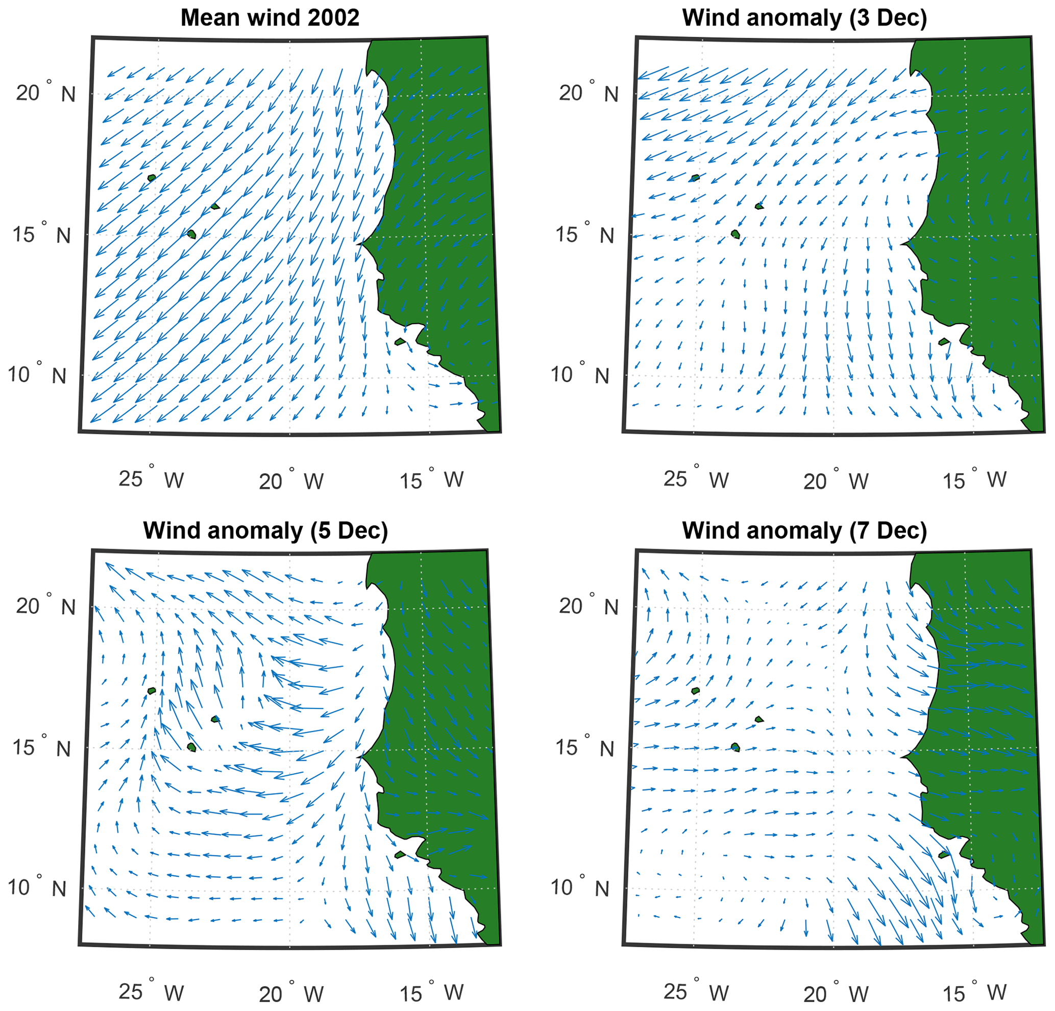
Figure 3Mean wind velocity in December 2002 (maximum ≃8 m s−1) and wind velocity anomaly on 3, 5, and 7 December (maximum ≃4 m s−1).
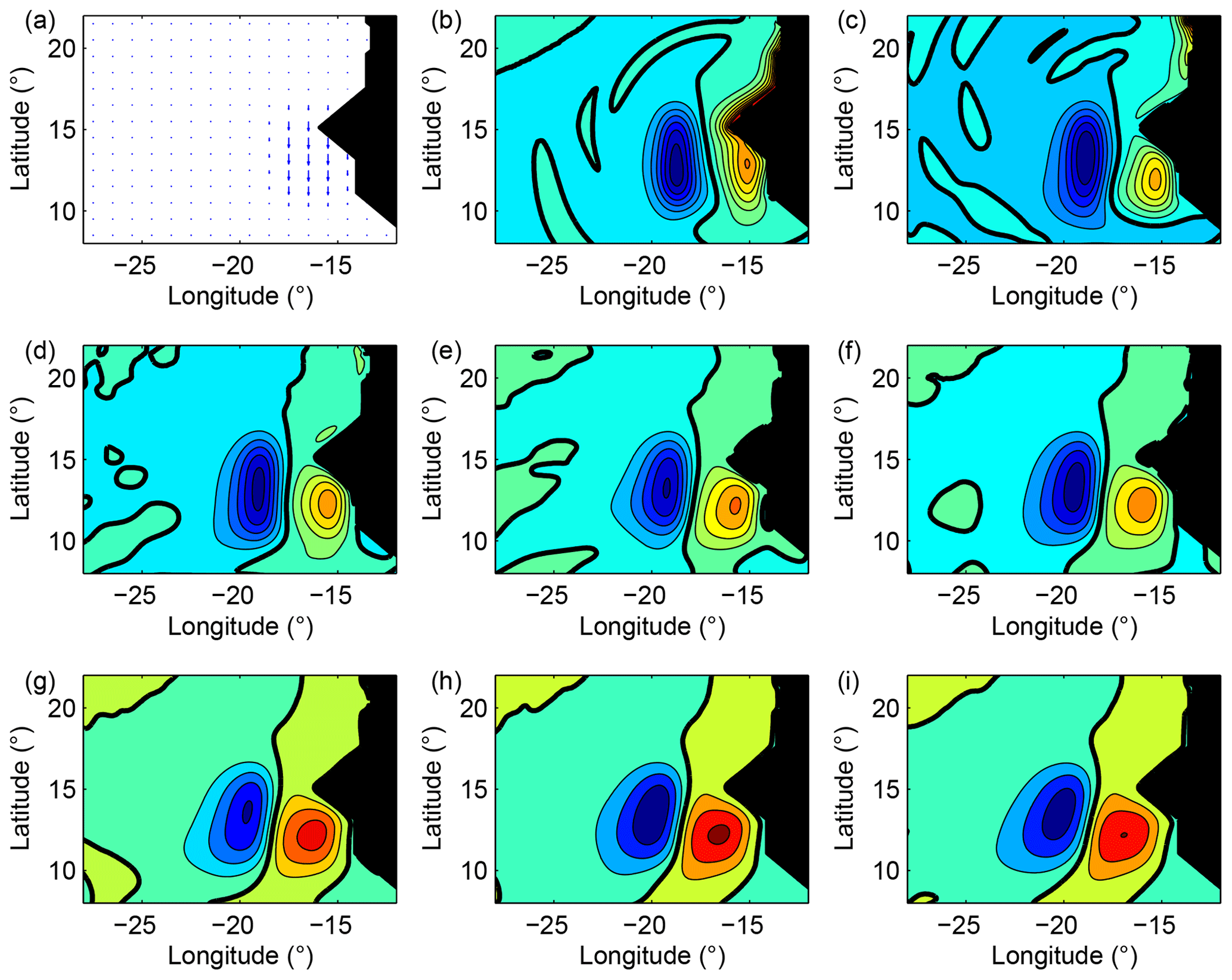
Figure 4Response of the ocean to an anomalous wind stress applied for 5 d (a) and corresponding evolution of the active layer thickness for every 5 d from the close of the wind stress anomaly up to 35 d after (b–i). A Rossby wave is generated and a Kelvin wave quickly propagates along the coast. The Rossby wave propagates westward and its amplitude is divided by 2 between (a) and (i). The 0 m isoline is indicated in bold; the isoline interval is 0.5 m (blue: negative).
3.2 Numerical resolution
The model domain is closed and centred at 15∘ N, the latitude of the Cape Verde Peninsula; it has a latitudinal extent of 20∘ and a longitudinal extent of 30∘. The peninsula is modelled as indicated in Fig. 4 in order to mimic the geometry of the coast of Senegal (simplified and smoothed). The mean value of h0 is equal to 200 m and the reduced gravity g⋆ to 0.02 m s−2. Consequently the Rossby radius of deformation at the latitude of the Cape Verde Peninsula is equal to 53 km.
The previous equations are solved by finite differences on a C-mesh on the sphere, the mesh size being equal to in longitudinal and latitudinal directions. The spatial scheme preserves enstrophy, following Sadourny (1975). No-slip boundary conditions are applied everywhere (including along the artificial boundaries which limit the open ocean). There is no added dissipation in the continuity equations and mass is conserved by the numerical scheme. The time integration is performed using a leapfrog scheme with a time step of 300 s. The viscosity ν and the coefficient r of Eq. (2) are respectively equal to 28 and m s−1 ( month). More details can be found in Février et al. (2007), where the two-layer version of this model is described.
3.3 Numerical set-up of the model
In Fig. 3 the mean wind for the considered period (December 2002–January 2003) is shown. It exemplifies the situation which is normally found in this region. The wind regularly blows from the north–north-east with a velocity ranging from 4 to 8 m s−1. To take this into account, a constant mean wind stress of amplitude equal to 0.06 N m−2 (corresponding to a mean wind velocity of about 5 m s−1 and a value of τ0 equal to m2 s−2) and oriented along a south–south-west direction is applied from rest for 4 years until a stationary mean state, which verifies the theoretical relation given in Sect. 3.1, is reached.
As shown by Fig. 3, a wind anomaly was active when the wave of Fig. 1 begins to be observed. This anomaly is obviously transient, but to the south of the Cape Verde Peninsula, it mainly points southwards. To represent this situation in a simplified way, in a first experiment we defined a north–south wind stress anomaly which extends over approximately 500 km and whose maximum is still equal to 0.06 N m−2. This anomaly is applied for 5 d (see Fig. 4a). The integration is continued for 45 d, after the anomaly has disappeared.
To explore the sensibility of the model response to the wind anomaly, others wind anomalies were applied (see below, in particular Figs. 6 to 8). The results obtained for these anomalies are discussed in the next section.
3.4 Numerical results
After the wind stress anomaly corresponding to the first experiment has vanished, the subsequent states of the ocean are shown every 5 d in Fig. 4 in terms of the active layer thickness. A coastal Kelvin wave forms north of the cape and quickly propagates along the coast. After 5 d, it has already gone beyond 25∘ N and after 10 d only the remains of the wave are still visible. South of the cape, a well-marked (Rossby) wave develops. Its size more or less matches the size of the wind stress anomaly. It slowly propagates westwards with a velocity of about 4 cm s−1. The amplitude of the wave decreases quickly because of the large value of h∕r. The minimum value of h is about −3.5 m when the wind ceases (panel b) and reaches only −2 m after 25 d (panel g).
These characteristics are actually those of a Rossby wave locally generated by a wind anomaly and then freely propagating in the open ocean. The wavelength of this wave is about 750 km ( m−1). Such a value is compatible with the theoretical study presented in Sect. 4 when the period of the wave is about 100 d. This modelled response to a wind stress anomaly also matches the satellite-observed signal described in the previous section. It thus suggests that the latter is the consequence of the existence of a Rossby wave generated by a wind burst.
Though the duration of the wind burst is short in our numerical experiment (5 d), the response of the system privileges a much longer timescale, exceeding 2 months. This result is not inconsistent. Indeed, the Fourier transform of a rectangular pulse is the sine-cardinal function. It thus contains a significant amount of energy at low frequencies and thus can generate a low-frequency response like the one observed here.
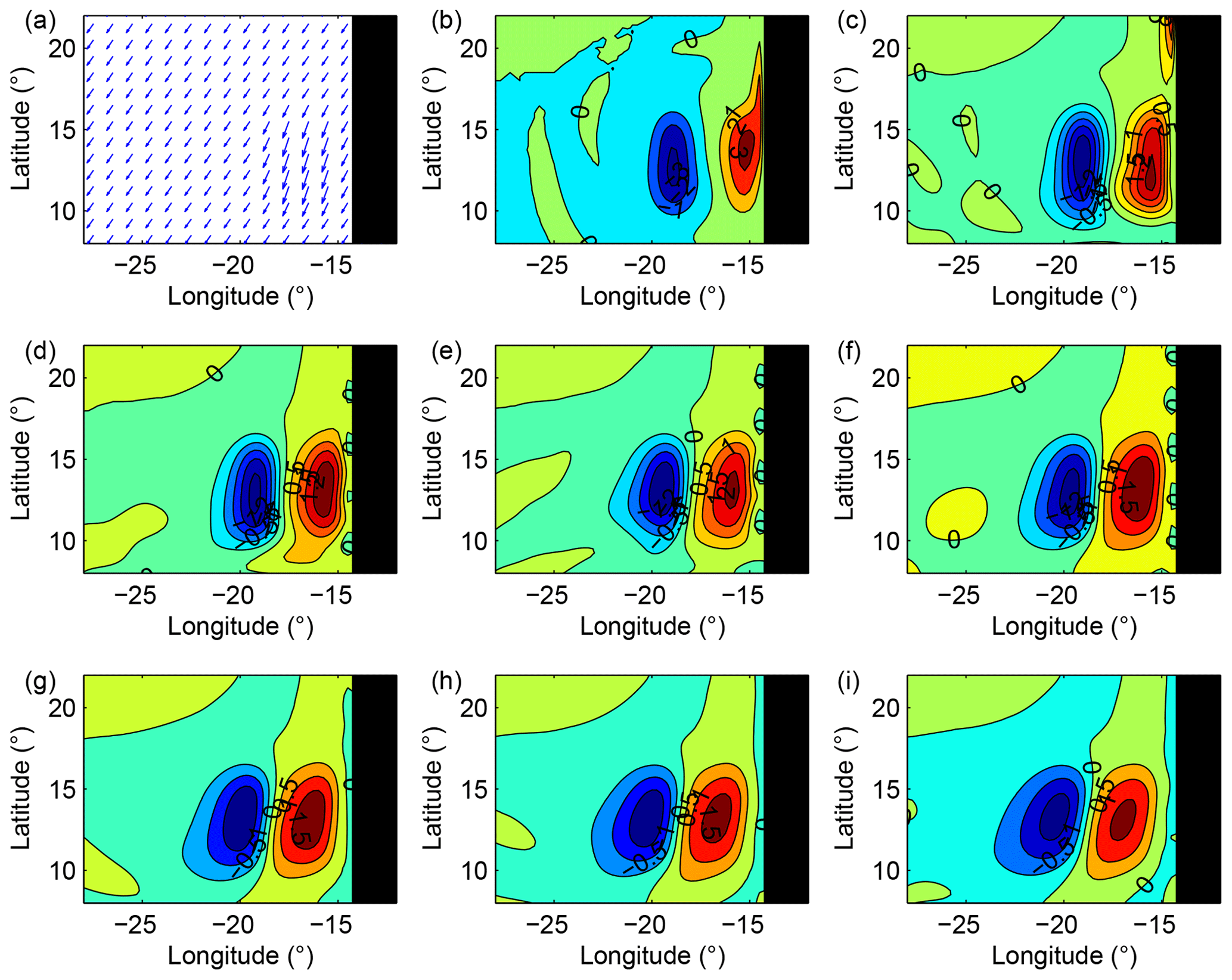
Figure 5Solution obtained for the same conditions as in Fig. 4 for a straight coastline. Note that the mean wind stress is added to the wind stress anomaly in panel (a). A Rossby wave is still generated, but the halting of the signal due to the cape is no longer observed. The latitudinal extent of the wave east of 19∘ W is thus nearly twice larger than in the previous case.
Figure 5 shows the results obtained in a similar experiment in which the cape is absent. The response of the model is very similar: in the area of the wind anomaly, a Kelvin wave forms and then quickly disappears, whereas a more persistent Rossby wave slowly propagates westward. However, the meridional extent of the Rossby wave is broader east of 18∘ W, in the area where the cape was previously. This suggests that the cape simply limits the extent of the wave northward but does not modify its dynamics. The theoretical study of Sect. 4 will confirm that the role of the cape remains moderate at low frequency.
A question arises: why does the wave have such a wavelength? Numerical experiments clearly show that the longitudinal wavelength is defined by the spatial scale of the forcing anomaly. This is first illustrated in Fig. 6, which shows the response of the model to a wind burst whose extent is 4 times smaller than the initial wind burst of Fig. 4. The latitudinal and longitudinal extent of the model response are approximately divided by 2 as expected. No Kelvin wave of significant amplitude is generated because there are no longer any wind anomalies on the coast; indeed, the centre of the wind anomaly is unchanged in comparison with the reference experiment. We will show in Sect. 4 that the period associated with the wave is increased when the wavelength is reduced (reaching approximately 150 d).
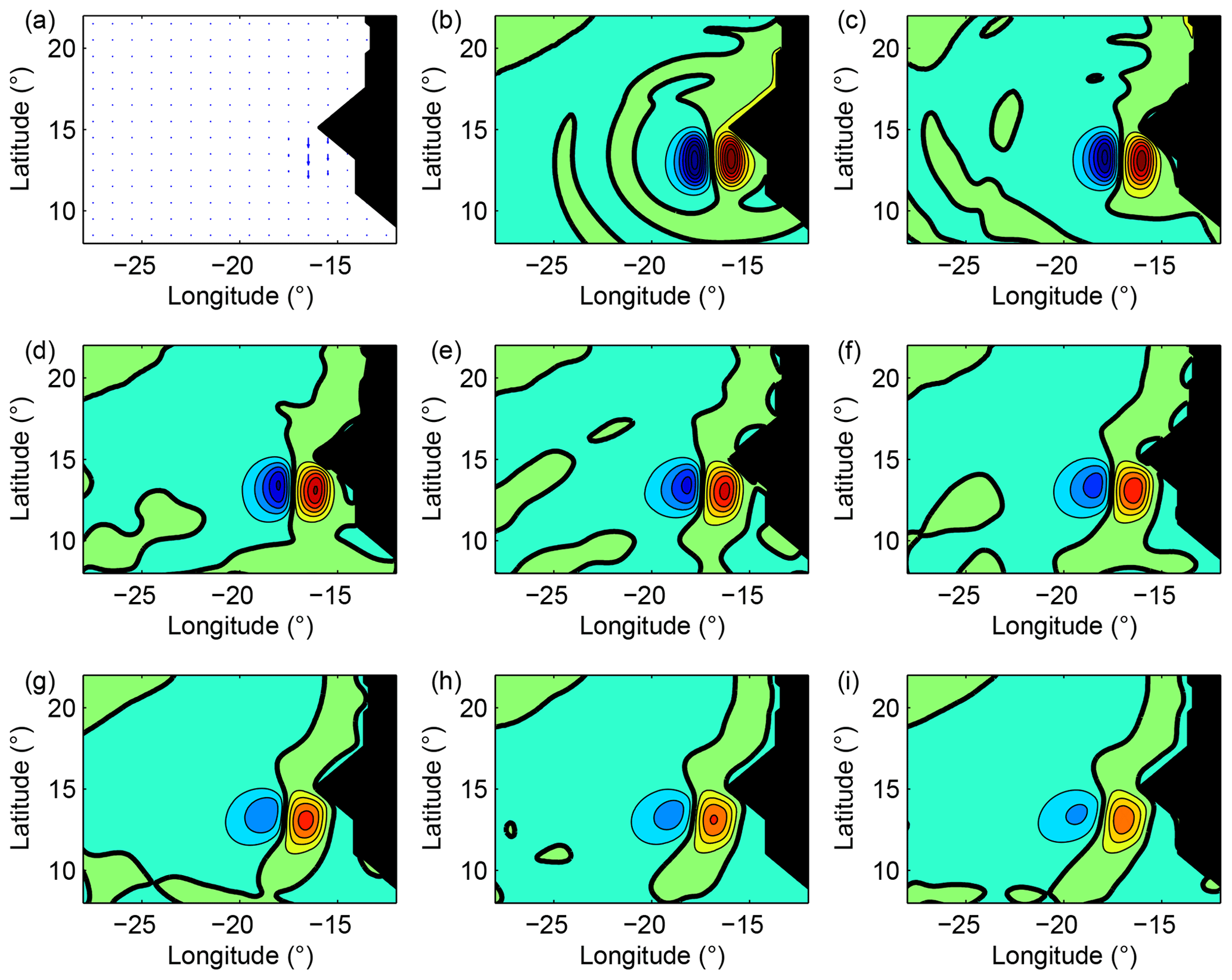
Figure 6The wind anomaly extent is 4 times smaller than the one used in Fig. 4 and the position of the centre is kept unchanged (a). It still acts for 5 d, and as previously the active layer thickness is shown for every 5 d from the close of the wind stress anomaly up to 35 d after. A Rossby wave is generated and its extent is approximately 4 times smaller than previously. No Kelvin waves are created. The 0 m isoline is indicated in bold; the isoline interval is 0.5 m (blue: negative).
Two supplementary experiments (Figs. 7 and 8) were carried out, in which a wind burst of large longitudinal (about 1000 km) and small latitudinal (about 100 km) extent is applied for 5 d; the anomaly is centred at 14∘ N in one case and 17∘ N in the other (see Figs. 7a and 8a). These anomalies create a Rossby wave with a large zonal extent. However, the response of the model differs in the two cases. When the anomaly is located south of the cape, a Kelvin wave is generated and a negative anomaly appears between 26 and 20∘ W. However, no positive anomaly with a comparable amplitude can be seen closer to the coast. A weak signal appears after day 20, but its extent is very small and its amplitude is 4 times smaller than the amplitude of the anomaly observed around 25–27∘ W. South of 14∘, a wave of small amplitude is created and propagates southward. Its latitudinal wavelength is comparable with the latitudinal extent of the wind anomaly. When the wind anomaly is located north of the cape, a negative anomaly appears between 26 and 20∘ W as previously; besides, a positive anomaly can be seen from day 5 and its amplitude is half the amplitude of the signal observed around 25–27∘ W.
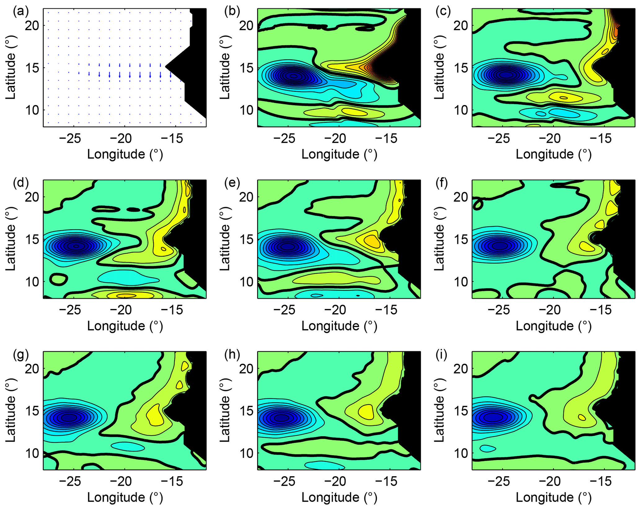
Figure 7The wind anomaly now acts over a long (1000 km) and narrow (200 km) domain south of the cape for 5 d (a). The solution after the close of the wind burst is shown. A wave is generated, but the anomaly remains moderate near the coast. The 0 m isoline is indicated in bold; the isoline interval is 0.1 m (blue: negative).
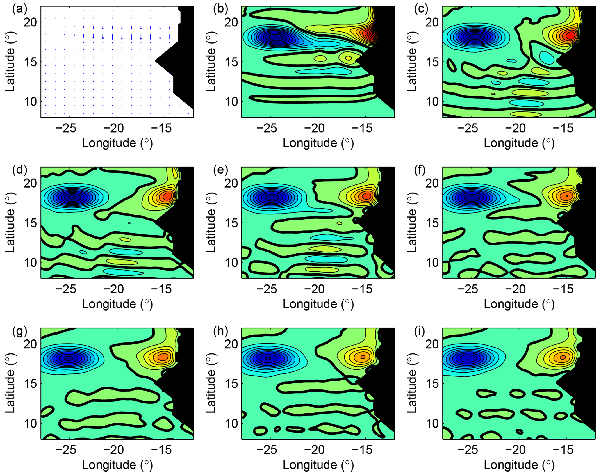
Figure 8The wind anomaly now acts over a long (1000 km) and narrow (200 km) domain north of the cape for 5 d (a). The solution after the close of the wind burst is shown. A wave is generated and the anomaly near the coast has an amplitude comparable with the anomaly around 25∘ W. The 0 m isoline is indicated in bold; the isoline interval is 0.1 m (blue: negative).
Clearly the response of the model close to the cape depends on the location of the wind anomaly, north or south of the cape. When the latter acts south of the cape, the anomaly which forms around 15∘ W is small and quickly disappears; a wave which propagates southward seems to prevent its existence. By contrast, when the wind anomaly acts north of the cape, an anomaly forms around 15∘W and gets stuck in this place; the wave which propagates southward still exists but its amplitude is about twice smaller than in the previous case. In the next section, we analytically investigate this dissymmetric behaviour in an idealized case.
In this section, we aim to understand whether the coastline may influence the propagation of the Rossby waves which are created close to the coast and propagate towards the open sea. The impact of the coastline has been investigated by Crépon and Richez (1984), Clarke (1977), and Clarke and Shi (1991) for the Kelvin waves using an analytical approach. Here we focus on the Rossby waves; as we consider an area which extends up to about 1000 km from the coast, we have to generalize the approach followed by Clarke and Shi, which introduced a local system of coordinates dependent of the coastline to study Kelvin waves along an irregular coastline. We try to answer the following questions:
- a.
Are there timescales for which the impact of the coastline (small in the numerical experiments) becomes more important?
- b.
A dissymmetry between the response north and south of the cape was visible in the numerical experiments; can this dissymmetry be dependent on the existence of the cape?
The analysis begins by defining and building a system of coordinates that permits us to follow the coastline geometry. This procedure is a standard one in mathematics when boundaries are complex; indeed, the boundary conditions can be written simply, which constitutes a substantial advantage. However, it has a drawback: the differential equations which characterize the problem become slightly more complex because they must include geometrical factors that take into account the deformation associated with the new system of coordinates. This drawback is small in comparison with the advantage.
When these new equations are established, straightforward calculations are made to obtain a unique partial differential equation (Eq. 7), which characterizes the evolution of η (the thickness of the active layer). This equation is a wave equation. Consequently the ray theory (or equivalently the Wentzel–Kramers–Brillouin method) can be applied. When the forcing terms are neglected, this yields a first-order non-linear differential Eq. (11). No new ideas are introduced after this. We just rewrite Eq. (11) by introducing new notations, in order to facilitate its study and the presentation of the results (end of Sect. 4.2). We then describe the results when the transport along the coast is much larger than the transverse transport (Sect. 4.3).
4.1 A model for the Kelvin and Rossby waves
We consider a reduced-gravity shallow-water model in the β plane forced by a constant wind stress which derives from a potential ϕ0(x,y) (), as in Sect. 3. Numerical integrations have shown that the exact solution v=0 and are actually obtained after a few years' integration (see Sect. 3.1 and 3.3).
If an anomaly (τx,τy) is added to the mean forcing τ0, a perturbation is generated; it is characterized by a depth anomaly h (the thickness of the first layer is now h0+h) and a velocity v. A linear approximation is sufficient to study the first steps of the evolution of the perturbation if the forcing anomaly remains moderate. The anomaly (τx,τy) can be written in terms of a potential and a stream function ,
so that the divergent part of the forcing is given by −Δϕ and the rotational part by Δψ.
The equations verified by the anomalies h and v are thus
The role of the diffusion and dissipation will not be considered below – a smoothing and damping of the solution is expected when it is taken into account. The previous system may be further simplified by introducing the zonal and meridional transports Tx=h0u and Ty=h0v and a potential η equal to . It becomes
where is a function of x and y.
These equations apply inside the ocean domain, whatever its shape. A boundary condition is added along the domain frontier (the normal transport vanishes), but the latter is difficult to handle when the shape of the coast is complex. Lastly, the spatial mean value of the depth anomaly h remains null.
The propagation of a Kelvin wave along the eastern boundary and the possible generation of Rossby waves can be studied by using a system (Eq. 5). Here, we consider an eastern boundary whose angle with the meridians varies smoothly, and we seek to understand how these variations may affect the wave dynamics. We consider only the case of a cape, even though the method could be applied in other cases. A coordinate change is made in order to “straighten the coast” and therefore have a simple boundary condition; Eq. 5 is correspondingly modified to match the new coordinates.
A new orthogonal system of coordinates and is thus introduced such that the eastern boundary is now defined by the simple equation X=0 (rather than a complex one such as ). In the local orthonormal basis eX,eY associated with this coordinates system, the line element dl reads
where a and b are geometrical factors which convey the stretching of the coordinates along orthogonal directions (note that the relations
where the initial coordinates x and y are now functions of the new coordinates X and Y, are used to compute a and b).
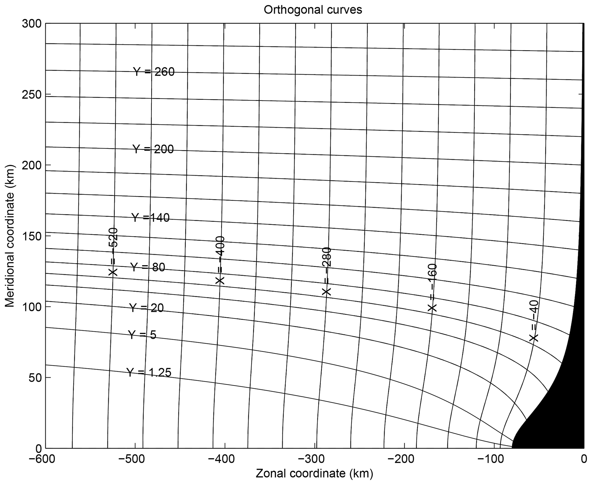
Figure 9Example of orthogonal coordinates X and Y defined for a cape protruding from the coast into the sea over a distance of 80 km. Several values of X and Y have been indicated. Only one half of the domain has been represented.

Figure 10The coefficients a and b are given for the coordinate system of Fig. 9 (they have no dimension).
Such a coordinate change is illustrated in Fig. 9 for a cape protruding into the sea over a distance of 80 km. Only half of the symmetric domain is shown. The initial coordinates x and y are the zonal and meridional coordinates; the new coordinates X and Y are represented in the original system and some of their values are indicated. Other coordinate changes would be possible. The corresponding geometrical factors a and b are shown in Fig. 10. They differ from 1 in a close neighbourhood and to the west of the cape (a is equal to 0.1 around the extremity of the cape, whereas b reaches 40 at 300 km west of the cape). A detailed study of this example will be presented in Sect. 4.3.
Using the coordinates (X,Y), the system labelled as “Eq. (5)” (5) becomes
where F, C, TX and TY are functions of X and Y corresponding to f, c, Tx and Ty (the notations for η, ϕ and ψ have not been changed to enhance the readability, but these functions also depend on X and Y).
Note that we use a more complex system than the traditional one which is used for the study of the Kelvin waves and which neglects the variations in the transport perpendicular to the coast:
We use the complete system (6) because we study Rossby waves far from the coast, for which these hypotheses do not hold. Indeed, if the previous simplified system is used, the two terms and must be removed from Eq. (11) below. These terms include the geometrical factors a and b due to coordinate change, and we try to investigate which is the impact of such terms.
We now concentrate on processes whose timescale is much larger than 1 d. Moreover we consider only the evolution of free waves. This situation corresponds to the case numerically investigated in Sect. 3 and illustrated in Figs. 4–8: the wind stress anomaly that had created the depth anomalies has ceased to exist. With these hypotheses, system (6) can be reduced to the following equation, which characterizes the evolution of η:
where is the Rossby radius. The boundary condition at the eastern coast now reads
for all t>0 and Y. The details of the computations can be found in Appendix A.
When a and b are close to 1 and the coast has a south–north orientation (see Fig. 10), the new coordinate system is nearly similar to the original one; indeed F mainly depends on Y≃y only, and in those regions Eq. (7) thus simplifies to
We recognize the equation characterizing the propagation of waves in the β plane () for a shallow-water model. For a tilted coast the dependance of the Coriolis parameter as a function of X should be still taken into account. For spatial scales much larger than R0 and at low frequency, Eq. (9) can be further simplified. It becomes , which simply models the westward propagation of long Rossby waves.
The coefficient b decreases as one gets closer to the cape (see Fig. 10). An impact of the cape in the open sea may therefore be expected because of the terms proportional to and in Eq. (7).
4.2 Ray theory
When a wave propagates in a medium whose properties change spatially, it does not follow straight lines but more complex paths. Ray theory – or the Wentzel–Kramers–Brillouin approximation – is used to determine the paths followed by the waves in such a medium. It applies when the wavelength is smaller than the typical scale at which the properties of the medium vary. The spatial variations in the components k and l of the wave vectors are taken into account by introducing a complex function such as and . The potential η is then equal to
where it is assumed that , , , . As required by the theory, these inequalities ensure that the wavelength is smaller than the typical scale of variation in the system, here conveyed by R0, F, and the coefficients a and b. Except in a very close vicinity of the cape (distance smaller than around 10 km) and for the meridional wavelength in the area located between −50 and 50 km north and south of the cape and beyond 200 km west of the cape, these inequalities mean that several wave patterns must be visible in the considered domain. This condition is verified for the waves observed in the numerical experiments and for the waves considered below.
Considering these hypotheses, η is given from Eq. (10) in the neighbourhood of a point M0 of coordinates (X0,Y0) by the approximate expression
where and . The physical meaning of this solution is explicated by taking its real part:
The solution must not increase westward since it cannot become infinite, which implies kI<0. Note, however, that kI>0 is possible if this occurs only in a (small) bounded domain. For kR>0, the wave propagates westwards.
The values of k and l are obtained by computing the function θ from Eqs. (7) and (8). After simplifying them by using the hypotheses above, we find that θ verifies the approximate (eikonal or Hamilton–Jacobi) equation
with the boundary condition
at X=0.
To make the computations clearer we set
-
,
-
,
-
,
-
,
and the problem (11) associated with the boundary condition (12) is rewritten as the following system:
At the boundary, Eqs. (14) and (15) permit us to determine the values of z1 and z2 and hence of k and l. Indeed, the introduction of Eq. (15) in Eq. (14) leads to the equation
Setting , this equation can be rewritten as
where is the Joukowsky transform of z; WR and WI are given by the relations
Equation (16) is the dispersion relation of the wave at the boundary. The Joukowsky transform of ξ z1 (or equivalently of ) depends on the frequency ω, the mean state (through R0), the latitude (through F) and the geometry of the coast (through a and b).
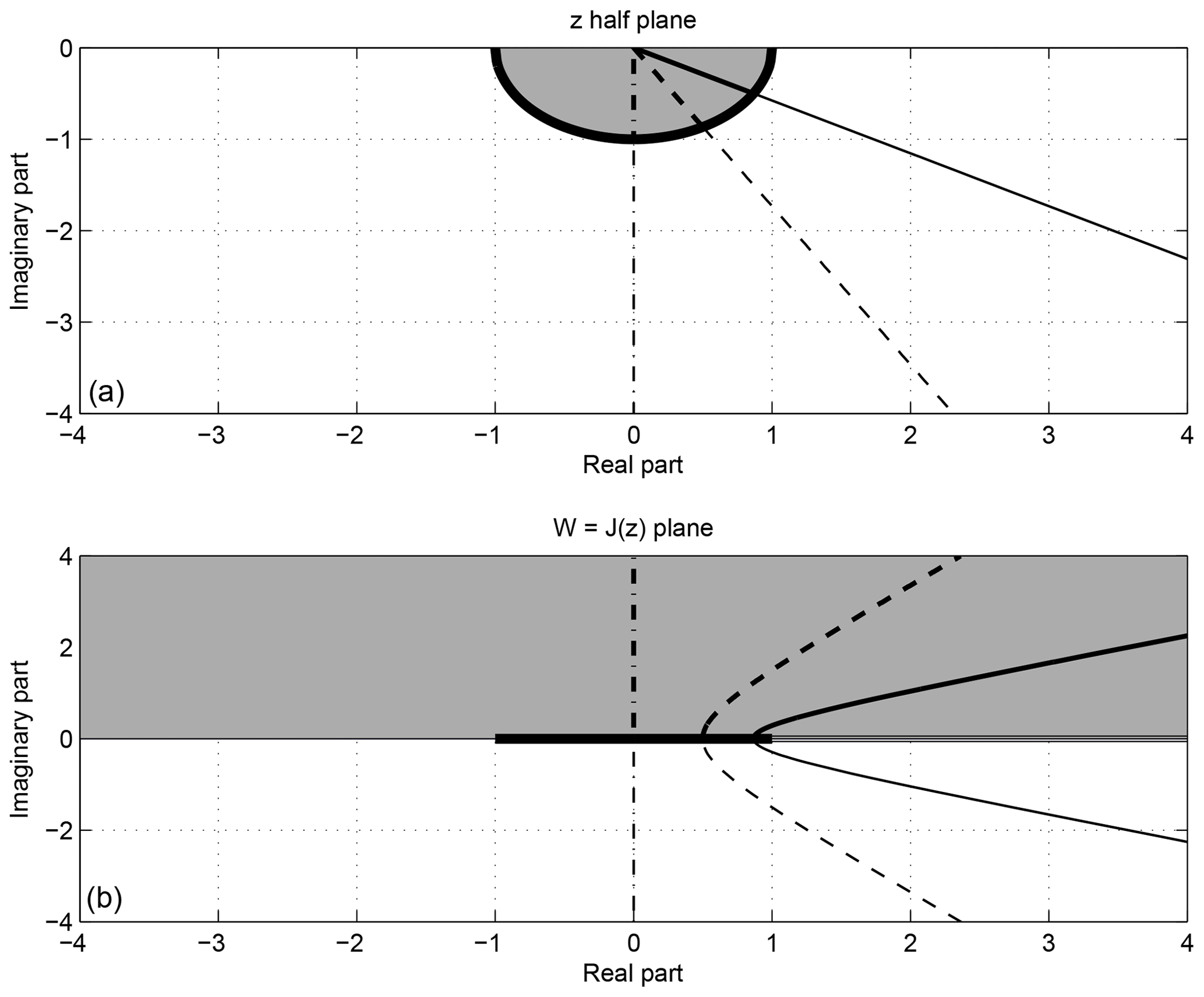
Figure 11In (a) the half complex plane ℑ(z)≤0 with z=ξz1 is shown. The domain is restricted to complex numbers with a negative imaginary part since must be negative. The half circle and a few straight lines have been drawn. In (b), the Joukowsky transform of the previous half plane W=J(z) is shown. The segment is the image of the half circle. The upper (lower) half plane corresponds to the image of its interior (exterior). The image of the straight lines is correspondingly represented.
The sketch in Fig. 11, which shows the half complex plane ℑ(z)<0 (panel a) and the complex plane W=J(z) (panel b), explains how the Joukowsky transformation works. The inferior half plane has been chosen since we expect kI<0 or in other words ℑ(z)<0.
-
When WI=ℑ(W) is positive, the complex number ξ z1 such as has a norm smaller than 1 (it corresponds to the grey areas in Fig. 11). The wavelength is thus large (). If WR=ℜ(W) is positive, the phase speed is negative (westward propagation).
-
When WI=ℑ(W) is negative, the complex number ξ z1 such as has a norm larger than 1 (it corresponds to the white areas). The wavelength is thus small. If WR=ℜ(W) is positive, the phase speed is still negative.
-
When WI vanishes, a situation which occurs when the coast is a straight line, the unique complex solution previously found can cease to exist. Indeed, if is smaller than 1, there is one complex solution whose norm is equal to 1 (on the half circle in bold in Fig. 11); and if is larger than 1, two real solutions are obtained (between and outside this interval). The case (WI=0) is detailed in the next subsection.
At the coast, relation (15) determines z2 when z1 is known. It implies that
For low frequencies ω∕F is much smaller than 1 and lI and lR can be ignored. An approximate expression of the waves is
and the dynamics are controlled by the westward propagation of Rossby waves. For shorter periods, the situation may be more complex because the ratio ωb∕(aF) may be close to 1. This effect is in agreement with the results obtained in Sect. 3, where a southward propagation of waves was observed in the open ocean, simultaneously with the westward propagation of Rossby waves.
Knowing z1 and z2 along the coast, it is possible to continue the resolution of the problem (Eqs. 13–14) and compute explicitly the rays characterizing the propagation of the waves. An algorithm which fulfils this objective is described in Appendix 2. However, under the supplementary assumption that remains much smaller than up to a distance from the coast of about a few Rossby radiuses of deformation, approximate expressions for z1 and z2 can be obtained analytically. This also permits us to initialize the algorithm described in Appendix B.
4.3 Analytical study for
In this case, Eq. (15), which is exact on the coast X=0, can also be used on a band of a few hundred kilometres off the coast and yields a good approximation of the solution (for a more detailed discussion, see Appendix 2). Consequently, Eq. (16) becomes valid over a domain which extends far off the coast in the open ocean. In this section, the consequences of this relation are briefly presented for a straight coastline and then investigated in detail for the cape shown in Fig. (9). In agreement with the hypotheses of the previous subsection, we assume that ω≪F, but the results and graphics will be produced up to the limit value ω=F.
4.3.1 Case of a straight coastline
This case has been extensively studied in the literature – for example, Richez et al. (1984), Grimshaw and Allen (1988), Clarke and Shi (1991), McCalpin (1995), and Liu et al. (1998); each article stresses a particular issue. Using the previously established equations, we here summarize known results about the existence of critical frequencies along an ocean boundary.
For a straight coastline following the south–north direction, we have X=x and Y=y; consequently, and F depends only on Y. Thus WI=0 and
where .
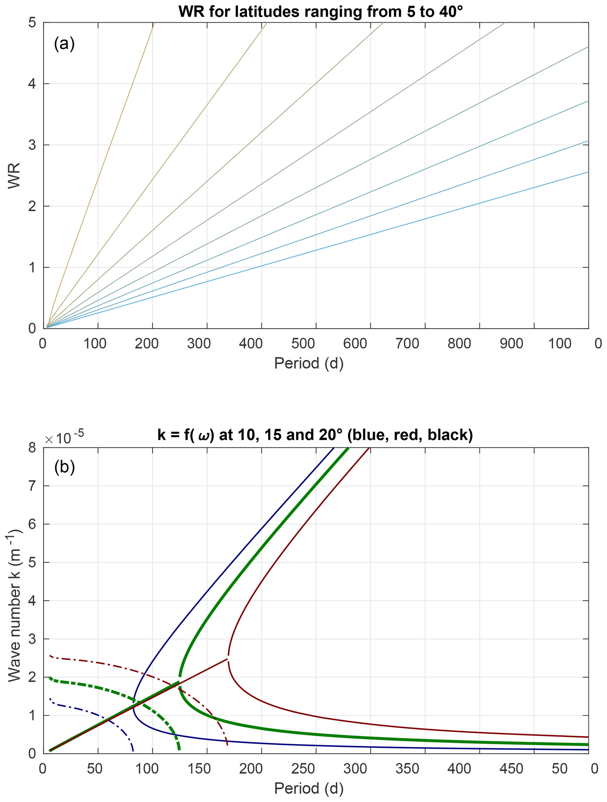
Figure 12(a) WR is shown for latitudes ranging from 5∘ N (left segment) to 40∘ N (right segment). The critical value WR=1 is reached at 15∘ N for a period of about 125 d. (b) Wavenumber k as a function of the period T for three different latitudes (10∘ (blue), 15∘ (red), and 20∘).
In Fig. 12a, the coefficient WR is shown at different latitudes as a function of the period. At 15∘ N, the critical value WR=1, which ensures the transition from a complex solution to two real solutions, is reached when the period is 140 d. Panel b shows the wavenumber as a function of the wave period computed from WR for 10∘ N (black), 15∘ N (grey) and 20∘ N (light grey). When WR>1, a condition which is always fulfilled at low frequency (characteristic time longer than 125 d at 15∘), Eq. (16) has two real solutions. If WR≫1, these solutions are close to and . Consequently, the wavenumber k is equal to either β∕ω or (see Eq. 16). This result proves the existence of Rossby waves, whose wavelength is either short or long. When the frequency increases, WR decreases and eventually reaches the critical value of 1. When WR becomes smaller than 1, there are two complex conjugate solutions. The only acceptable solution has a negative imaginary part and conveys the existence of a Kelvin wave, trapped along the coastline and propagating northward. The absolute value of this imaginary part kI is represented as a dashed curve in Fig. 12b. When the wave frequency is close to the critical value, kI vanishes and consequently the Kelvin wave no longer exists. A Rossby wave with a significant amplitude can propagate westwards. At 15∘ N its wavelength will be around 300 km. The zonal velocity (phase speed) of this non-dispersive wave is about 2.5 km d−1. On the other hand, as lR vanishes with kI, the meridional velocity becomes infinite.
Similar results are obtained when the coast presents a constant angle θ with a meridian. The only change is that the critical frequency for which the wave regime changes is modified and depends on the tilt of the coast as indicated in Clarke and Shi (1991).
4.3.2 Case of a cape
The wave dynamics in a neighbourhood of the cape are characterized by the coefficients WR and WI which convey the effect of the coastline on the propagation of the wave. The coefficient WR can be split into two terms; the first one is similar to the term obtained from a straight coastline, whereas the second one explains the role of the coast. It is large when ξ is small – in the frequency range where the model is valid, this means for wave periods going from ∼10 d to a month – and when the deformation of the coastline is large. The existence of such a term was expected. When the angle of the coastline with a meridian increases, the impact of the latitudinal variations in the Coriolis parameter decreases along the path followed by the wave. It even vanishes when the coast becomes parallel to the Equator. These changes are taken into account by this term. By contrast, at low frequency, the lengthening or shortening of the path followed by the wave becomes negligible because it occurs over a time which remains short in comparison with the period of the wave.
The variations in the coastline geometry also prevent the existence of two distinct solutions at low frequency. Indeed, WI differs from 0, and consequently two complex solutions are obtained as explicated in Fig. 11. If WI is strictly negative (grey area), the solution z is inside the half unit disc and kR is small. If WI is strictly positive, the solution is outside and kR is large. The degeneracy of the equation thus disappears, and a selection of the wavelength operates.

Figure 13Dimensionless coefficient WR for periods equal to 10, 20, 50 and 100 d. The bold black line corresponds to WR=0. When the period of the wave shortens (smaller than 20 d), WR becomes negative in a narrow band south of the cape. For period longer than 100 d, the diagram is nearly symmetric.
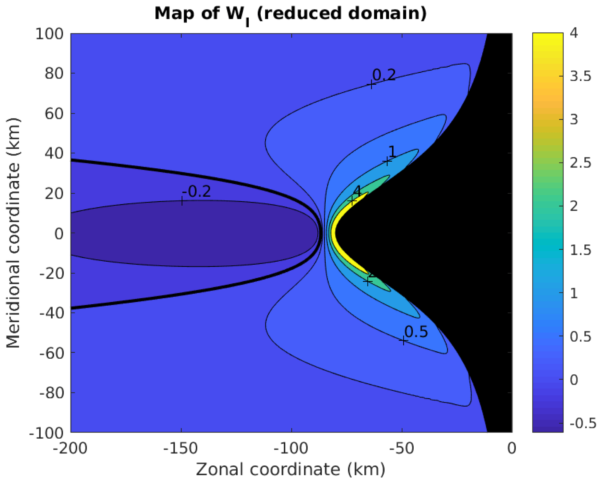
Figure 14Dimensionless coefficient WI. It is independent of the period of the wave. Note that the domain is reduced in comparison with the previous figure.
Figure 13 shows WR for T=10, 20, 50 and 100 d and makes visible an interesting property. When the period T is equal to 10 d, a dissymmetry around the cape occurs: WR is negative south and positive north of the cape. This dissymmetry weakens when the period increases. For T=20 d, the area where WR is negative is strongly reduced and for T=50 d, it has vanished. Since the signs of WR and kR are similar (see Fig. 11 and the associated comments), a negative kR is expected in this area and actually appears (see Fig. 15).
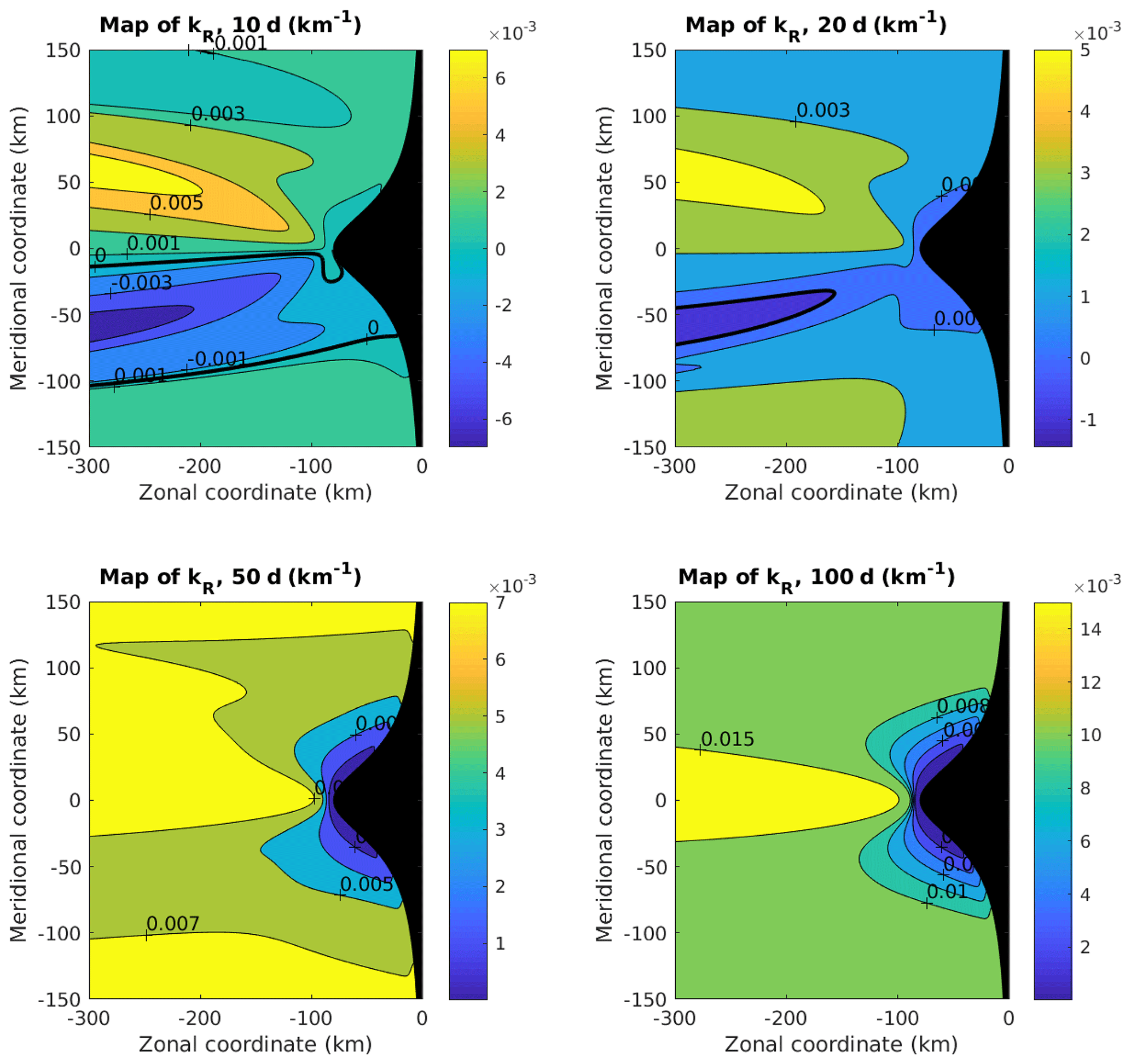
Figure 15Coefficient kR for periods equal to 10, 20, 50 and 100 d. The bold black line separates positive from negative values. Where WR is negative, kR is negative (for periods shorter than 20 d, in the area located to the south of the cape).
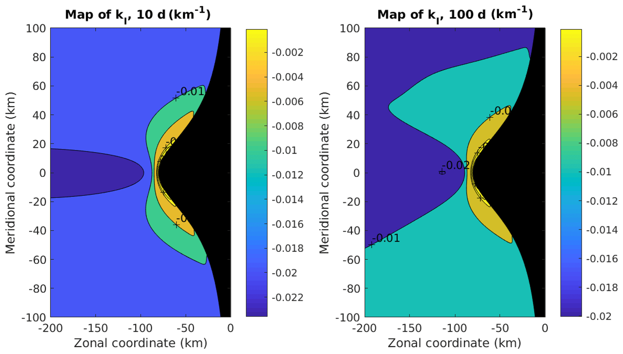
Figure 16Coefficient kI for periods equal to 10 and 100 d. This coefficient depends weakly on the period of the wave.
Since WI is nearly independent of the period in the considered frequency range, a single map suffices to describe it (Fig. 14). WI is positive everywhere except in a narrow area west of the cape (the isoline −0.2 is indicated and the bold line corresponds to WI=0). Figure 11 shows that the corresponding values of ξz1 are smaller than 1. This suggests that this area is occupied by waves whose wavelength is longer than everywhere else, a result which appears in Fig. 15.
The maps of kR and kI (see Figs. 15 and 16) show properties in agreement with the previous analysis. For periods shorter than 20 d, kR becomes negative south of the cape. Consequently the waves no longer propagate westward towards the open sea but eastward towards the coast. By contrast, north of the cape the propagation always occurs westward, whatever the frequency. At lower frequency this phenomenon is not observed. The coefficient kI shows a smaller dependence as a function of the period. The shape of the Kelvin wave is modified close to the tip of the cape – its offshore extent is smaller since kI is larger – but it still exists and propagates northwards.
Lastly, note that the order of magnitude predicted in Fig. 12 for a straight coastline with a south–north orientation is noticeably changed when the shape of the coast is taken into account. For a wavelength of about 700 km, the corresponding period was equal to approximately 150 d. Now, Fig. 15 shows that this wavelength is obtained in a large part of the domain for a period equal to 100 d. Note that this value is close to the values predicted by Clarke and Shi (1991) at the coast (between 84.69 and 115.2 d). Note also that, in a small area around the extremity of the cape (blue area), larger wavelengths are compatible with periods of about 100 d.
The analysis of SeaWiFS satellite observations of chlorophyll showed a well-marked signal along and off the west African coast, between 10 and 22∘ N, in winter (December to April). Along the coast the high concentration of chlorophyll is associated with the offshore Ekman drift generated by the equatorward component of the trade wind, which forces an upward motion. Its variability is modulated by Kelvin waves propagating northwards. In December 2002 and January 2003, we observed a wavelike pattern in the open sea, which extends far away offshore, up to a distance of about 800 km off the coast. This signal was visible from 20 December 2002 and was detectable for approximately 1 month, south of the Cape Verde Peninsula.
This pattern suggested the existence of locally generated Rossby waves, which slowly propagated westward. Indeed, such a wave can generate an elevation of the lower layers of the ocean corresponding to an upwelling of nutrient-rich water. The existence of this wave was confirmed by the study of the SSH signal coming from AVISO altimeter data. It evidenced a wave propagating westward with a velocity of about 4.5 cm s−1. The existence of a chlorophyll signal far from the coast – here extending up to 750 km west to the Cape Verde Peninsula – has to our knowledge never been described. This strongly differs from the coastal signals associated with Kelvin waves, which have been previously carefully analysed (see Diakhaté et al., 2016, and the references therein).
In this study we thus investigated the mechanisms which could lead to the existence of such a wave and analysed the potential role of the cape, by first doing numerical experiments with a forced non-linear model, then by analytically studying a linear reduced-gravity model.
The numerical study, based on a reduced-gravity shallow-water model, showed that a Rossby wave similar to the observed pattern could be created by a wind burst broadly extending over the region where the oceanic signal was seen. This agreed with wind reanalysis of this period. In our experiments a longshore wind burst which lasted 5 d was used to generate the oceanic response. We showed that the spatial scale of the latter matches the spatial scale of the forcing. The timescale of the response, controlled by the wavelength (see below), is not that of the forcing (5 d) but much longer around 100 d for the first experiment.
The cape does not seem to modify the basic features of the wave dynamics. It mainly limits the extent of the wave to the north. However, when the wind burst has a large zonal extent (of about 1000 km) and a small meridional extent (not exceeding 100 km), the response of the model close to the cape depends on the location of the wind anomaly. When the latter acts south of the cape, the anomaly which forms around 15∘ W is small and quickly disappears; a wave which propagates southward seems to prevent its existence. By contrast, when the wind anomaly acts north of the cape, an anomaly forms and remains around 15∘ W, without moving; a secondary wave which propagates southward still exists but disappears quickly.
The analytical study is new and extends the study of Clarke and Shi (1991) to the open sea up to a distance of about 1000 km away from the coast. It helps us interpret the numerical results and gives further information. It first shows that a timescale around 100 d can be associated with the observed wave, considering the value of the wavelength (around 700 km). This value matches the critical value predicted by Clarke and Shi along the coast of Senegal, even though their model applied only at the coast when the angle defining the tilt of the coastline is not too large. It also shows that the role of the cape does not dramatically modify the dynamics of the system at such timescales.
By contrast, when the period becomes shorter (smaller than 20–30 d), the waves behave differently north and south of the cape, as suggested by the numerical experiments. For the studied set-up, Rossby waves can propagate eastwards, in a narrow band of the ocean whose latitudinal extent is about 100 km. We verified that this property vanished when the cape flattened (the period of the wave progressively becoming shorter). This strongly suggests that the wave dynamics in the vicinity of a cape – and the associated upwelling – depend on the geometry of the coastline for timescales shorter than 1 month. These changes no longer matter for longer timescales. Note that the behaviour difference predicted by the theory is not so important in the numerical experiments. This is not surprising since the geometry of the system is different in the numerical experiments.
This study thus suggests that offshore upwellings can be created or enhanced by Rossby waves. An example of such a phenomenon has been observed in the region off Senegal. This example is probably not unique. For instance Kounta et al. (2018) show patterns which provide clear evidence of an important Rossby wave activity to the south of the Cape Verde Peninsula (see, for example, their Fig. 10, which shows a climatology of the volume meridional transport). Observations will have to be pursued in this region and in other EBUS region to determine the importance of such events. However, the observations of such a structure by satellite require several conditions which seldom occur together. First we need a long period of observations without clouds, second a typical wind event able to generate the Rossby wave, and third the existence of nutrients in the subsurface layers, which could enrich the surface layers.
An important problem is the detectability of these waves. Dealing with a reduced-gravity model whose characteristics fit the observations, we found that the elevation of the interface probably does not exceed a few metres. The interface elevation facilitates the nutrient enrichment of the surface layers and consequently favours phytoplankton blooms. As the elevation of the interface is relatively small, the phytoplankton bloom is likely to occur only under very specific conditions such as a relatively small average thermocline depth or the presence of phytoplankton species capable of rapid growth, with a strong chlorophyll signature like diatoms. In fact, phytoplankton pigment retrieval from ocean colour satellite observation shows that the chlorophyll signal we observed is dominated by fucoxanthin, which is a signature of diatoms (Khalil et al., 2019)
The water-leaving reflectances were obtained from the SeaWiFS daily reflectances provided by NASA/GSFC/DAAC (https://oceancolor.gsfc.nasa.gov/data/seawifs/, last access: December 2019) observed at the top of the atmosphere (TOA). The atmospheric correction was reprocessed at LOCEAN (Farikou et al., 2015). The reflectances are available at the following website: http://poacc.locean-ipsl.upmc.fr/ (last access: April 2019). The altimeter products are available from AVISO (Archiving, Validation, and Interpretation of Satellite Oceanographic) at https://www.aviso.altimetry.fr/ (last access: December 2019). We used gridded sea level heights and derived variables (types of dataset: Ssalto/Duacs gridded multi-mission altimeter products). The Ssalto/Duacs altimeter products are produced and distributed by the Copernicus Marine and Environment Monitoring Service (CMEMS) (http://marine.copernicus.eu; last access: July 2019). The wind data are available at the following address: https://www.ecmwf.int/en/forecasts/datasets/reanalysis-datasets/era-interim (last access: December 2019). They come from the global atmospheric reanalysis that is available from 1 January 1979 to 31 August 2019 (see the report by Berrisford, P., Dee, D.P., Poli, P., Brugge, R., Fielding, M., Fuentes, M., Kållberg, P.W., Kobayashi, S., Uppala, S., published in 2011 at https://www.ecmwf.int/node/8174; last access: July 2019). The data can also be made available upon request to the authors.
Since we consider processes whose timescale is larger than a day, Eq. 6 can be simplified. We define a characteristic frequency ω0 and a daily frequency Fd and assume that they verify . Setting ω0t=τ and F=FdF0, the first two equations of system (6) become
with and . An elementary computation leads to the following relations:
Considering our hypothesis, the terms of order 1 and ϵ can be kept in the previous equations and the terms of order ϵ2 can be neglected. Consequently we can use the approximate relations
(We used the fact that and F0Fd=F.) Note that the terms ∂tRX and ∂tRY are of order ϵ in comparison with the terms FRY and FRX.
We now introduce these equations in the last equation of system (6). This leads to a new equation:
or equivalently
where is the Rossby radius and Rψ contains the forcing terms depending on ψ:
The vanishing of the velocity orthogonal to the coordinates is easily obtained from system (A3). With the same approximations, the condition TX=0 at X=0 implies or equivalently
for all t>0 and Y.
When the forcing terms can be neglected, the previous relations simplify. They become
and at X=0, for all t>0 and Y,
A method to solve system (13–14) with the boundary condition (15) is presented here. It has been shown that the values of z1 and z2 are known at the boundary thanks to Eq. (16). We set
where and verifies Eq. (14), and the condition everywhere. Consequently, verifies Eq. (16) everywhere,
and can be computed on the ocean domain. The results of this computation are presented in Sect. 4.3 ( is also known thanks to the relation ).
Since z1 and z2 are known on the coast and and everywhere, and are known on the coast X=0. It is now easy to write the equations verified by and .
with and for X=0.
The variables and can be computed on a grid for , . They are known for X=0 (i=0). We suppose that they have been computed for i>0 (values and ) and show how and can be computed. Equation (B1) can be discretized in the following way:
the error being proportional to ΔX. A boundary condition (for example, ) is prescribed to end the computation. Knowing , the value of is obtained by solving
The computation of and would correspond to a solution such as TX=0 everywhere. The correction brought by and is associated with a mass transport perpendicular to the coast. As the latter in general is much smaller than the transport TY parallel to the coast, it is expected that and are small in comparison with and (they are null at X=0 and increase proportionally to the distance to the coast). In Sect. 4.3, the approximate value of k associated with the solution is fully described.
MC provided the satellite analysis. JS made the numerical simulation. The paper benefitted from input from all the authors
The authors declare that they have no conflict of interest.
We thank Xavier Capet for fruitful discussions, for his careful reading of the paper and pertinent comments. We thank Rémi Tailleux and Jacyra Soares for their precise and constructive reviews, which permitted us to improve this article greatly.
This paper was edited by Neil Wells and reviewed by Remi Tailleux and Jacyra Soares.
Allen, J. S.: Some aspects of the forced wave response of stratified coastal regions, J. Phys. Oceanorgr., 6, 113–119, 1976.
Batteen, M. L.: Wind-forced modeling studies of currents, meanders, and eddies in the California Current System, J. Geophys. Res., 102, 985–1009, 1997.
Capet, X., McWilliams, J., Molemaker, M., and Shchepetkin, A.: Mesoscale to submesoscale transition in the California current system: flow structure, eddy flux, and observational tests, J. Phys. Oceanogr., 28, 29–43, 2008a.
Capet, X., McWilliams, J., Molemaker, M., and Shchepetkin, A.: Mesoscale to submesoscale transition in the California current system: Frontal processes. J. Phys. Oceanogr., 28, 44–64, 2008b.
Capet, X., Estrade, P., Machu, É., Ndoye, S., Grelet, J., Lazar, A., Marié, L., Dausse, D., and Brehmer, P.: On the dynamics of the southern Senegal upwelling center; Observed variability from synoptic to superinertial scales, J. Phys. Oceanogr., 47, 155–180, https://doi.org/10.1175/JPO-D-15-0247.1, 2017.
Castelao, R. M. and Bart, J. A.: Upwelling around Cabo Frio, Brazil: The importance of wind stress curl, Geophys. Res. Lett., 33, L03602, https://doi.org/10.1029/2005GL025182, 2006.
Clarke, A. J.: Wind forced linear and nonlinear Kelvin waves along an irregular coastline, J. Fluid Mech., 83, 337–348, 1977.
Clarke, A. J.: The reflection of equatorial waves from ocean boundaries, J. Phys. Oceanogr., 13, 1193–1207, 1983.
Clarke, A. J. and Shi, C.: Critical frequencies at ocean boundaries. J. Geophys. Res., 96, 10731–10738, 1991.
Crépon, M. and Richez, C.: Transient upwelling generated by two dimensional atmospheric forcing and variability in the coastline, J. Phys. Oceanogr., 12, 1437–1457, 1982.
Crépon, M., Richez, C., and Chartier, M.: Effects of coastline geometry on upwellings, J. Phys. Oceanorgr., 14, 1365–1382, 1984.
Demarcq, H. and Faure V.: Coastal upwelling and associated retention indices from satellite SST. Application to Octopus vulgaris recruitment, Oceanogr. Acta, 23, 391–407, 2000.
Diakhaté, M., de Coëtlogon, G., Lazar, A., and Gaye, A. T.: Intraseasonal SST variability within tropical Atlantic upwellings, Q. J. Roy. Meteor. Soc., 14, 372–386, 2016.
Enriquez, A. G. and Friehe, C. A.: Effects of wind stress and wind stress curl variability ob coastal upwelling, J. Phys. Oceanorgr., 25, 1551–1571, 1995.
Farikou, O., Sawadogo, S., Niang, A., Brajard, J., Mejia, C., Crépon, M., and Thiria, S.: Multivariate Analysis of the Senegalo-Mauritanian Area by Merging Satellite Remote Sensing Ocean Color and SST Observations, Res. J. Environ. Earth Sci., 5, 756–768, 2013.
Farikou, O., Sawadogo, S., Niang, A., Diouf, D., Brajard, J., Mejia, C., Dandonneau, Y., Gasc, G., Crépon, M., and Thiria, S.: Inferring the seasonal evolution of phytoplankton groups in the Senegalo-Mauritanian upwelling region from satellite ocean-color spectral measurements, J. Geophys. Res.-Oceans, 120, 6581–6601, https://doi.org/10.1002/2015JC010738, 2015.
Février S., Sirven, J., and Herbaut, C.: Interaction of a coastal Kelvin wave with the mean state in th Gulf Stream separation area, J. Phys. Oceanorgr., 37, 1429–1444, 2007.
Gill, A. E. and Clarke, A. J.: Wind-induced upwelling, coastal currents and sea level changes, Deep-Sea Res., 21, 325–345, 1974.
Grimshaw, R. and Allen, J. S.: Low frequency baroclinic waves off coastal boundaries, J. Phys. Oceanorgr., 18, 1124–1143, 1988.
Kounta, L., Capet, X., Jouanno, J., Kolodziejczyk, N., Sow, B., and Gaye, A. T.: A model perspective on the dynamics of the shadow zone of the eastern tropical North Atlantic – Part 1: the poleward slope currents along West Africa, Ocean Sci., 14, 971–997, https://doi.org/10.5194/os-14-971-2018, 2018.
Lachkar, Z. and Gruber, N.: A comparative study of biological production in eastern boundary upwelling systems using an artificial neural network, Biogeosciences, 9, 293–308, https://doi.org/10.5194/bg-9-293-2012, 2012.
Lachkar, Z. and Gruber, N.: Response of biological production and air-sea CO2 fluxes to upwelling intensifications in the California and Canary Current Systems, J. Mar. Syst., 109–110, 149–160, https://doi.org/10.1016/j.jmarsys.2012.04.003, 2013.
Lathuillière, C., Échevin, V., and Lévy, M.: Seasonal and intraseasonal surface chlorophyll-a variability along the northwest African coast, J. Geophys. Res., 113, C05007, https://doi.org/10.1029/2007JC004433, 2008.
Marchesiello, P. and Estrade, P.: Eddy activity and mixing in upwelling systems: a comparative study of Northwest Africa and California regions, Int. J. Earth. Sci., 98, 299–308, https://doi.org/10.1007/s00531-007-0235-6, 2009.
Marchesiello, P., McWilliams, J. C., and Shchepetkin, A.: Equilibrium structure and dynamics of the California current system, J. Phys. Oceanogr., 33, 753–783, 2003.
McCalpin, J. D.: Rossby wave Generation by poleward propagating Kelvin waves: the midlatitude quasigeostrophic approximation, J. Phys. Oceanogr., 25, 1415–1425, 1995.
McCreary, J. P.: A linear stratified ocean model of the coastal undercurrent, Philos. T. Roy. Soc. Lond., A202, 385–413, 1981.
McCreary, J. P. and Kundu, P. K.: Western boundary circulation driven by an alongshore wind; With application to the Somali Current system, J. Mar. Res., 43, 493–516, 1985.
McCreary, J. P., Shetye, S. R., and Kundu, P. K.: Thermohaline forcing of eastern boundary currents: with application to the circulation off the west coast of Australia, J. Mar. Res., 44, 71–92, 1986.
Moore, D. W.: Planetary-gravity waves in an equatorial ocean, PhD thesis, 201 pp., Harvard Univ., Cambridge, Mass, 1968.
Ndoye S., Capet, X., Estrade, P., Sow, B., Dagorne, D., Lazar, A., Gaye, A., and Brehmer, P.: SST patterns and dynamics of the Southern Senegal-Gambia upwelling center, J. Geophys. Res.-Oceans, 119, 8315–8335, https://doi.org/10.1002/2014JC010242, 2014.
Pickett, M. H. and Paduan, J. D.: Ekman transport and pumping in the California current based on the U.S. Navy's high-resolution atmospheric model (COAPMPS), J. Geophys. Res., 108, C103327, https://doi.org/10.1029/2003JC001902, 2003.
Richez, C., Philander, G., and Crépon, M.: Oceanic response to coastal winds with shear, Oceanol. Acta, 7, 409–416, 1984.
Sadourny, R.: The dynamics of finite difference models of the shallow water equations, J. Atmos. Sci., 32, 680–689, 1975.
Sawadogo, S., Brajard, J., Niang, A., Lathuilier̀e, C., Crépon, M., and Thiria S.: Analysis of the Senegalo-Mauritanian upwelling by processing satellite remote sensing observations with topological maps, Proceedings IEEE International Joint Conference on Neural Networks, IJCNN, 2826–2832, Atlanta, USA, 2009.
Schopf, P. S., Anderson, D. L. T., and Smith, R.: Beta-dispersion of low-frequency Rossby waves, Dyn. Atmos. Oceans, 5, 187–214, 1981.
Yala, K., Niang, N., Brajard, J., Mejia, C., Ouattara, M., El Hourany, R., Crépon, M., and Thiria, S.: Estimation of phytoplankton pigments from ocean-color satellite observations in the Sénégalo-Mauritanian region by using an advanced neural classifier, Ocean Sci. Discuss., https://doi.org/10.5194/os-2019-11, in review, 2019.