Victor A. Miroshnikov
Department of Mathematics, College of Mount Saint Vincent, New York, USA.
DOI: 10.4236/ajcm.2020.101004   PDF    HTML   XML   372 Downloads   862 Views   Citations

Abstract

An exact 3-D solution for deterministic chaos of J wave groups with M internal waves governed by the Navier-Stokes equations is presented. Using the Helmholtz decomposition, the Dirichlet problem for the Navier-Stokes equations is decomposed into the Archimedean, Stokes, and Navier problems. The exact solution is derived by the method of decomposition in invariant structures (DIS). A cascade differential algebra is developed for four families of invariant structures: deterministic scalar kinematic (DSK) structures, deterministic vector kinematic (DVK) structures, deterministic scalar dynamic (DSD) structures, and deterministic vector dynamic (DVD) structures. The Helmholtz decomposition of anticommutators, commutators, and directional derivatives is computed in terms of the dot and cross products of the DVK structures. Computation is performed with the help of the experimental and theoretical programming in Maple. Scalar and vector variables of the Stokes problem are decomposed into the DSK and DVK structures, respectively. Scalar and vector variables of the Navier problem are expanded into the DSD and DVD structures, correspondingly. Potentialization of the Navier field is possible since internal vortex forces, which are described by the vector potentials of the Helmholtz decomposition, counterbalance each other. On the contrary, external potential forces, which are expressed via the scalar potentials of the Helmholtz decomposition, superpose together to form the gradient of a dynamic pressure. Various constituents of the kinetic energy and the total pressure are visualized by the conservative, multi-wave propagation and interaction of three-dimensional, nonlinear, internal waves with a two-fold topology, which are called oscillons and pulsons.

Keywords

The Navier-Stokes Equations, Internal Waves, Decomposition into Invariant Structures, Experimental and Theoretical Programming, Conservative Multi-Wave Interaction

Share and Cite:

1. Introduction

Conservative interaction of N three-dimensional internal waves controlled by the Navier-Stokes equations has been studied in [1], where the existence theorem is proved for a partial solution of the correspondent boundary-value problem via the Stationary Kinematic Euler-Fourier (SKEF) functions. However, an extreme sophistication of the partial solution derived with the help of experimental and theoretical programming in Maple doesn’t permit development of a general solution for propagation and interaction of wave groups of internal waves.

To overcome this challenge, a structural approach to this problem has been developed in [2], where the differential algebra of SKEF structures is studied and various applications of the SKEF structures for solving the Laplace equation and the Helmholtz equations are considered. Here, the method of Decomposition in Invariant Structures (DIS) is systematically developed to solve various kinematic (linear) problems of computing the Helmholtz decomposition.

The objective of the current paper is a continuation of the structural approach towards development of a cascade of dynamic (nonlinear) invariant structures, which permit the computation of the exact general three-dimensional solution for propagation and interaction of J wave groups with M internal waves per group.

The contents of this paper are following. Experimental Deterministic Scalar Kinematic (DSK) structures, which are the revised SKEF structures of [2], are systematically considered and complemented by theoretical DSK structures in Section 2. The experimental and theoretical DSK structures, which are used to solve the kinematic problem for scalar fluid-dynamic variables, generate experimental and theoretical Deterministic Vector Kinematic (DVK) structures, which are studied in Section 3 and are utilized to find vector variables of the kinematic problem. To compute scalar variables of the dynamic problem, experimental and theoretical Deterministic Scalar Dynamic (DSD) structures are defined with the help of the relevant DSK structures in Section 4 and the differential algebra of the DSD structures is treated, as well. In Section 5, experimental and theoretical DSK and DVK structures are combined to produce and develop experimental and theoretical Deterministic Vector Dynamic (DVD) structures for vector variables of the dynamic problem. The section concludes with the Helmholtz decomposition of directional derivatives of the DVK structures. The Helmholtz decomposition of the Navier-Stokes problem into the Archimedean, Stokes, and Navier problems is tackled in Section 6, where the general solution of the Stokes problem is expanded in the theoretical DSK and DVK structures. The general solution for deterministic chaos of J wave groups with M internal waves is completed in Section 7, where the dynamic variables are decomposed in the theoretical DSD and DVD structures. Section 8 deals with the orthogonal and non-orthogonal decompositions of the kinetic energy between wave groups and internal waves. Here, exponential oscillons and pulsons, which are novel nonlinear conservative solutions for propagation and interaction of various constituents of the kinetic energy and the total pressure, are introduced and visualized. The most interesting properties of the DSK, DVK, DSD, and DVD structures are discussed in Section 9 together with important properties of the general solution. Directions of further exploration of the deterministic chaos of internal waves are also outlined there.

2. Scalar Kinematic Structures

Scalar kinematic structures $s_{i,m}=\left[s_{1,m},s_{2,m},s_{3,m},s_{4,m}\right]=\left[a_m,b_m,c_m,d_m\right]$ have been constructed in [1] and later developed in [2] as the SKEF structures. In a modified notation, the non-orthogonal normalized structural basis of four Deterministic Scalar Kinematic (DSK) structures becomes

$\begin{array}{l}{s}_{1,m}=a_m=+A{v}_{m}ss{e}_m+B{v}_{m}cs{e}_m+C{v}_{m}sc{e}_m+D{v}_{m}cc{e}_m,\\ s_{2,m}=b_m=-B{v}_{m}ss{e}_m+A{v}_{m}cs{e}_m-D{v}_{m}sc{e}_m+C{v}_{m}cc{e}_m,\\ s_{3,m}=c_m=-C{v}_{m}ss{e}_m-D{v}_{m}cs{e}_m+A{v}_{m}sc{e}_m+B{v}_{m}cc{e}_m,\\ s_{4,m}=d_m=+D{v}_{m}ss{e}_m-C{v}_{m}cs{e}_m-B{v}_{m}sc{e}_m+A{v}_{m}cc{e}_m,\end{array}$ (1)

where $i=1,2,\cdots ,J$ is an index of a structural wave group generated by the DSK structure $s_{i,m}$ , $m=1,2,\cdots ,M$ is an index of a harmonic wave, M is a total number of harmonic waves in the structural wave group, functional coefficients $\left[A{v}_m,B{v}_m,C{v}_m,D{v}_m\right]$ , which do not depend on the independent Cartesian coordinates (x, y, z) and time t, are functional amplitudes of a harmonic variable v(x, y, z, t). The functional amplitudes are normalized by

$A{v}_m^2+B{v}_m^2+C{v}_m^2+D{v}_m^2=1$ (2)

In the general solution, $J=4$ and $J=1,2,3$ in partial solutions.

In Equation (1), the DSK functions $f_{i,m}=\left[f_{1,m},f_{2,m},f_{3,m},f_{4,m}\right]=[ss{e}_m,cs{e}_m,sc{e}_m,cc{e}_m]$ are defined as follows:

$\begin{array}{l}{f}_{1,m}=ss{e}_m=\sin \left({\kappa }_m{X}_m\right)\sin \left({\lambda }_m{Y}_m\right)\exp \left({\left(-1\right)}^{\sigma }{\mu }_{m}z\right),\\ f_{2,m}=cs{e}_m=\cos \left({\kappa }_m{X}_m\right)\sin \left({\lambda }_m{Y}_m\right)\exp \left({\left(-1\right)}^{\sigma }{\mu }_{m}z\right),\\ f_{3,m}=sc{e}_m=\sin \left({\kappa }_m{X}_m\right)\cos \left({\lambda }_m{Y}_m\right)\exp \left({\left(-1\right)}^{\sigma }{\mu }_{m}z\right),\\ f_{4,m}=cc{e}_m=\cos \left({\kappa }_m{X}_m\right)\cos \left({\lambda }_m{Y}_m\right)\exp \left({\left(-1\right)}^{\sigma }{\mu }_{m}z\right),\end{array}$ (3)

where $\left[{\kappa }_m,{\lambda }_m,{\mu }_m\right]$ are wave parameters related by the Pythagorean identity

${\kappa }_m^2+{\lambda }_m^2={\mu }_m^2.$ (4)

In Equations (3), the dependent Cartesian coordinates

$\begin{array}{l}{X}_m=x-U_{m}t+X_{0,m},\\ Y_m=y-V_{m}t+Y_{0,m}\end{array}$ (5)

include x- and y-components of the velocity $\left[U_m,V_m,0\right]$ of a Cartesian frame moving with the mth wave and coordinates $\left[X_{0,m},Y_{0,m},0\right]$ of the origin (x, y, z) = (0, 0, 0) of the motionless frame in the mth moving frame at the initial moment t = 0. In an upper domain,

$U=\left[x\in \left(-\infty ,\infty \right),y\in \left(-\infty ,\infty \right),z\in \left(0,\infty \right)\right],$ (6)

a decay parameter

$\sigma =1$ (7)

and, in a lower domain,

$L=\left[x\in \left(-\infty ,\infty \right),y\in \left(-\infty ,\infty \right),z\in \left(-\infty ,0\right)\right],$ (8)

$\sigma =0$ . (9)

All wave parameters $\left[{\kappa }_m,{\lambda }_m,{\mu }_m\right]$ , $\left[U_m,V_m\right]$ , and $\left[X_{0,m},Y_{0,m}\right]$ of the DSK functions do not depend on (x, y, z) and t, as well.

If $A{v}_m=1,B{v}_m=0,C{v}_m=0,D{v}_m=0$ , the DSK structures (1) are reduced to the DSK functions (3) as

$\begin{array}{l}{s}_{1,m}=a_m=ss{e}_m=f_{1,m},\\ s_{2,m}=b_m=cs{e}_m=f_{2,m},\\ s_{3,m}=c_m=sc{e}_m=f_{3,m},\\ s_{4,m}=d_m=cc{e}_m=f_{4,m}.\end{array}$ (10)

It is a straightforward matter to show completeness of the DSK structures (1) with respect to differentiation in (x, y, z) of any order [1] [2] since

$\begin{array}{l}\frac{\partial a_m}{\partial x}=+{\kappa }_m{b}_m,\text{}\text{}\text{}\frac{\partial a_m}{\partial y}=+{\lambda }_m{c}_m,\text{}\frac{\partial a_m}{\partial z}={\left(-1\right)}^{\sigma }{\mu }_m{a}_m,\\ \frac{\partial b_m}{\partial x}=-{\kappa }_m{a}_m,\frac{\partial b_m}{\partial y}=+{\lambda }_m{d}_m,\frac{\partial b_m}{\partial z}={\left(-1\right)}^{\sigma }{\mu }_m{b}_m,\\ \frac{\partial c_m}{\partial x}=+{\kappa }_m{d}_m,\frac{\partial c_m}{\partial y}=-{\lambda }_m{a}_m,\frac{\partial c_m}{\partial z}={\left(-1\right)}^{\sigma }{\mu }_m{c}_m,\\ \frac{\partial d_m}{\partial x}=-{\kappa }_m{c}_m,\frac{\partial d_m}{\partial y}=-{\lambda }_m{b}_m,\frac{\partial d_m}{\partial z}={\left(-1\right)}^{\sigma }{\mu }_m{d}_m.\end{array}$ (11)

The first derivatives of the DSK structures $\left[a_m,b_m,c_m,d_m\right]$ in (x, y) are covariant since they are proportional to costructures in the x- and y-directions, respectively. The first derivatives of the DSK structures with respect to z are invariant because they are proportional to themselves.

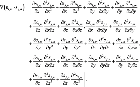
The first spatial derivatives of the DSK structure $s_{i,m}$ are visualized in Figure 1. Differentiation in x and y moves the DSK structure $s_{i,m}=\left[a_m,b_m,c_m,d_m\right]$ from one corner of a differentiation rectangle to another one, while differentiation in z does not change a location of $s_{i,m}$ . For each invariant structure $s_{i,m}$ ,

there is a costructure in the x-direction $s_{i,m,cx}=\left[b_m,a_m,d_m,c_m\right]$ , which is located on the same horizontal leg at a distance $\pm {\kappa }_m$ given by the coefficient of a relevant derivative. There is also a costructure in the y-direction $s_{i,m,cy}=\left[c_m,d_m,a_m,b_m\right]$ , which is located on the same vertical leg at a distance $\pm {\lambda }_m$ , which is provided by the coefficient of a correspondent derivative. Differentiation in z is invariant with the invariable coefficient ${\left(-1\right)}^{\sigma }{\mu }_m$ since differentiation in z doesn't change the location of $s_{i,m}$ . Thus, the differentiation diagram demonstrates transformation of the DSK structures produced by differentiation, which is shown by blue arrows for derivatives in x, by green arrows for derivatives in y, and red arrows for derivatives in z. The length of arrows of derivatives in (x, y, z) are proportional to differentiation scales $\left[{\kappa }_m,{\lambda }_m,{\left(-1\right)}^{\sigma }{\mu }_m\right]$ , which are shown with colors corresponding to those of arrows.

By a tedious calculation, it may be shown that the differentiation table of the first spatial derivatives of the theoretical DSK structures $\left[s_{i,m},s_{i,m,cx},s_{i,m,cy},s_{i,m,cx,cy}\right]$ takes the following form:

$\begin{array}{l}\frac{\partial s_{i,m}}{\partial x}=+{\left(-1\right)}^{{\alpha }_i}{\kappa }_m{s}_{i,m,cx},\text{}\text{}\text{}\frac{\partial s_{i,m}}{\partial y}=+{\left(-1\right)}^{{\beta }_i}{\lambda }_m{s}_{i,m,cy},\\ \frac{\partial s_{i,m}}{\partial z}={\left(-1\right)}^{\sigma }{\mu }_m{s}_{i,m},\frac{\partial s_{i,m,cx}}{\partial x}=-{\left(-1\right)}^{{\alpha }_i}{\kappa }_m{s}_{i,m},\\ \frac{\partial s_{i,m,cx}}{\partial y}=+{\left(-1\right)}^{{\beta }_i}{\lambda }_m{s}_{i,m,cx,cy},\frac{\partial s_{i,m,cx}}{\partial z}={\left(-1\right)}^{\sigma }{\mu }_m{s}_{i,m,cx},\\ \frac{\partial s_{i,m,cy}}{\partial x}=+{\left(-1\right)}^{{\alpha }_i}{\kappa }_m{s}_{i,m,cx,cy},\frac{\partial s_{i,m,cy}}{\partial y}=-{\left(-1\right)}^{{\beta }_i}{\lambda }_m{s}_{i,m},\\ \frac{\partial s_{i,m,cy}}{\partial z}={\left(-1\right)}^{\sigma }{\mu }_m{s}_{i,m,cy},\frac{\partial s_{i,m,cx,cy}}{\partial x}=-{\left(-1\right)}^{{\alpha }_i}{\kappa }_m{s}_{i,m,cy},\text{}\text{}\text{}\\ \frac{\partial s_{i,m,cx,cy}}{\partial y}=-{\left(-1\right)}^{{\beta }_i}{\lambda }_m{s}_{i,m,cx},\frac{\partial s_{i,m,cx,cy}}{\partial z}={\left(-1\right)}^{\sigma }{\mu }_m{s}_{i,m,cx,cy}.\end{array}$ (12)

Connections between the theoretical DSK structures and the experimental DSK structures (1) and the corresponding values of the sign parameters ${\alpha }_i$ and ${\beta }_i$ are

$\begin{array}{l}{s}_{1,m}=a_m,s_{1,m,cx}=b_m,s_{1,m,cy}=c_m,s_{1,m,cx,cy}=d_m,{\alpha }_1=0,{\beta }_1=0,\\ s_{2,m}=b_m,s_{2,m,cx}=a_m,s_{2,m,cy}=d_m,s_{2,m,cx,cy}=c_m,{\alpha }_2=1,{\beta }_2=0,\\ s_{3,m}=c_m,s_{3,m,cx}=d_m,s_{3,m,cy}=a_m,s_{3,m,cx,cy}=b_m,{\alpha }_3=0,{\beta }_3=1,\\ s_{4,m}=d_m,s_{4,m,cx}=c_m,s_{4,m,cy}=b_m,s_{4,m,cx,cy}=a_m,{\alpha }_4=1,{\beta }_4=1.\end{array}$ (13)

The table of definitions (13) is complemented by a table of oscillation properties of the DSK costructures and the sign parameters of higher orders

$\begin{array}{l}{s}_{i,m,cx,cx}=s_{i,m},s_{i,m,cx,cy}=s_{i,m,cy,cx},s_{i,m,cy,cy}=s_{i,m},\\ s_{i,m,cx,cy,cx}=s_{i,m,cy},s_{i,m,cx,cy,cy}=s_{i,m,cx},\\ {\left(-1\right)}^{{\alpha }_{i,cx}}=-{\left(-1\right)}^{{\alpha }_i},{\left(-1\right)}^{{\alpha }_{i,cy}}=+{\left(-1\right)}^{{\alpha }_i},{\left(-1\right)}^{{\alpha }_{i,cx,cy}}=-{\left(-1\right)}^{{\alpha }_i},\\ {\left(-1\right)}^{{\beta }_{i,cx}}=+{\left(-1\right)}^{{\beta }_i},{\left(-1\right)}^{{\beta }_{i,cy}}=-{\left(-1\right)}^{{\beta }_i},{\left(-1\right)}^{{\beta }_{i,cx,cy}}=-{\left(-1\right)}^{{\beta }_i}.\end{array}$ (14)

The experimental DSK structures $\left[a_m,b_m,c_m,d_m\right]$ present a fixed notation of the corner points of the differentiation rectangle in Figure 1 and the theoretical DSK structures $\left[s_{i,m},s_{i,m,cx},s_{i,m,cy},s_{i,m,cx,cy}\right]$ represent a floating notation of the vertices of the differentiation diagram. The differentiation table (12) shows equivalence of the theoretical DSK structures with respect to the spatial differentiation of the first order since each of the theoretical DSK structures may be used to obtain the experimental derivatives (11). The described comparison of the theoretical and experimental results shows a quadrality of the theory, i.e. there are four equivalent theoretical ways of explaining the experimental results. It may be shown that the quadrality of the theoretical DSK structures holds with respect to the second spatial derivatives, the Laplacians, and the first temporal derivatives, as well. For the aim of brevity, further theoretical results will be demonstrated mainly for the theoretical DSK structure $s_{i,m}$ that is sufficient to describe experimental results.

Using the theoretical table (12) of the first spatial derivatives, we find the second derivatives of the theoretical DSK structure $s_{i,m}$ in (x, y, z)

$\begin{array}{l}\frac{{\partial }^2{s}_{i,m}}{\partial x^2}=-{\kappa }_m^2{s}_{i,m},\text{}\text{}\text{}\frac{{\partial }^2{s}_{i,m}}{\partial x\partial y}={\left(-1\right)}^{{\alpha }_i+{\beta }_i}{\kappa }_m{\lambda }_m{s}_{i,m,cx,cy},\text{}\\ \frac{{\partial }^2{s}_{i,m}}{\partial y^2}=-{\lambda }_m^2{s}_{i,m},\frac{{\partial }^2{s}_{i,m}}{\partial x\partial z}={\left(-1\right)}^{{\alpha }_i+\sigma }{\kappa }_m{\mu }_m{s}_{i,m,cx},\\ \frac{{\partial }^2{s}_{i,m}}{\partial z^2}=+{\mu }_m^2{s}_{i,m},\frac{{\partial }^2{s}_{i,m}}{\partial y\partial z}={\left(-1\right)}^{{\beta }_i+\sigma }{\lambda }_m{\mu }_m{s}_{i,m,cy}.\end{array}$ (15)

The differentiation diagram immediately explains invariance of the repeated second spatial derivatives. The second-order differentiation moves the DSK structure $s_{i,m}$ from any corner to another corner of the differentiation rectangle transforming $s_{i,m}$ to a costructure and then returns in back both in the x- and y-directions restoring the original value of $s_{i,m}$ . Similar to the physical oscillation, this effect of differentiation may be called a scalar structural oscillation.

Since the first derivative of the DSK structure $s_{i,m}$ with respect to z is invariant, the coefficient of the second derivative in z is positive because

${\left({\left(-1\right)}^{{\alpha }_i}\right)}^2={\left({\left(-1\right)}^{{\beta }_i}\right)}^2={\left({\left(-1\right)}^{\sigma }\right)}^2=1$ (16)

The coefficients of the second derivative of $s_{i,m}$ in (x, y) are negative since the first derivatives in (x, y) are covariant.

In agreement with the differentiation diagram (Figure 1), the second derivative of $s_{i,m}$ in (x, y) becomes a costructure $s_{i,m,cx,cy}$ in (x, y), which is located at an opposite vertex of the differentiation rectangle to that of $s_{i,m}$ . The second derivatives of $s_{i,m}$ in (x, z) and (y, z) become the costructures $s_{i,m,cx}$ and $s_{i,m,cy}$ in the x- and y-directions, respectively, since differentiation in z is invariant.

Summation of the repeated second derivatives of the differentiation table (15) of the second spatial derivatives shows that the theoretical DSK structure $s_{i,m}$ is harmonic, i.e.

$\left(-{\kappa }_m^2-{\lambda }_m^2+{\mu }_m^2\right)s_{i,m}=\Delta s_{i,m}=0$ (17)

because of the Pythagorean identity (4), where the Laplacian

$\Delta =\frac{{\partial }^2}{\partial x^2}+\frac{{\partial }^2}{\partial y^2}+\frac{{\partial }^2}{\partial z^2}$ . (18)

With the help of the chain rule, definitions (3) and (5), and the spatial derivatives (12), we find

$\frac{\partial s_{i,m}}{\partial t}=-{\left(-1\right)}^{{\alpha }_i}{U}_m{\kappa }_m{s}_{i,m,cx}-{\left(-1\right)}^{{\beta }_i}{V}_m{\lambda }_m{s}_{i,m,cy}.$ (19)

Expanding (19) for $i=1,2,3,4$ and using (13) yields that the experimental DSK structures $\left[a_m,b_m,c_m,d_m\right]$ are also closed with respect to temporal differentiation of any order. In view of Figure 1, we observe that the first derivative of the DSK structure $s_{i,m}$ in t is a superposition of the costructures $s_{i,m,cx}$ and $s_{i,m,cy}$ in the x- and y-directions, which are located in the adjacent corner points of the differentiation rectangle. Whereas structural amplitudes of the costructures depend on products $\left[U_m{\kappa }_m,V{\lambda }_m\right]$ of the propagation velocities and the wave numbers in the (x, y) plane.

3. Vector Kinematic Structures

Four experimental Deterministic Vector Kinematic (DVK) structures $s_{i,m}=[s_{1,m},s_{2,m},s_{3,m},s_{4,m}]=\left[a_m,b_m,c_m,d_m\right]$ are defined as gradients of the DSK structures (1) by

$\begin{array}{l}{s}_{1,m}=a_m=\nabla a_m=\left[+{\kappa }_m{b}_m,+{\lambda }_m{c}_m,{\left(-1\right)}^{\sigma }{\mu }_m{a}_{{}_m}\right],\\ s_{2,m}=b_m=\nabla b_m=\left[-{\kappa }_m{a}_m,+{\lambda }_m{d}_m,{\left(-1\right)}^{\sigma }{\mu }_m{b}_{{}_m}\right],\\ s_{3,m}=c_m=\nabla c_m=\left[+{\kappa }_m{d}_m,-{\lambda }_m{a}_m,{\left(-1\right)}^{\sigma }{\mu }_m{c}_{{}_m}\right],\\ s_{4,m}=d_m=\nabla d_m=\left[-{\kappa }_m{c}_m,-{\lambda }_m{b}_m,{\left(-1\right)}^{\sigma }{\mu }_m{d}_{{}_m}\right],\end{array}$ (20)

where the gradients are calculated in accordance with (11).

If $A{v}_m=1,B{v}_m=0,C{v}_m=0,D{v}_m=0$ , the DVK structures (20) are reduced to DVK functions, which are set as follows:

$\begin{array}{l}{s}_{1,m}=a_m=\nabla ss{e}_m=f_{1,m},\\ s_{2,m}=b_m=\nabla cs{e}_m=f_{2,m},\\ s_{3,m}=c_m=\nabla sc{e}_m=f_{3,m},\\ s_{4,m}=d_m=\nabla cc{e}_m=f_{4,m}.\end{array}$ (21)

Application of the gradient to the theoretical DSK structures $[s_{i,m},s_{i,m,cx},s_{i,m,cy},s_{i,m,cx,cy}]$ in the view of the differentiation table (12) results in the following definitions of the theoretical DVK structures:

$\begin{array}{l}{s}_{i,m}=\nabla s_{i,m}=\left[+{\left(-1\right)}^{{\alpha }_i}{\kappa }_m{s}_{i,m,cx},+{\left(-1\right)}^{{\beta }_i}{\lambda }_m{s}_{i,m,cy},{\left(-1\right)}^{\sigma }{\mu }_m{s}_{i,m}\right],\\ s_{i,m,cx}=\nabla s_{i,m,cx}=\left[-{\left(-1\right)}^{{\alpha }_i}{\kappa }_m{s}_{i,m},+{\left(-1\right)}^{{\beta }_i}{\lambda }_m{s}_{i,m,cx,cy},{\left(-1\right)}^{\sigma }{\mu }_m{s}_{i,m,cx}\right],\\ s_{i,m,cy}=\nabla s_{i,m,cy}=\left[+{\left(-1\right)}^{{\alpha }_i}{\kappa }_m{s}_{i,m,cx,cy},-{\left(-1\right)}^{{\beta }_i}{\lambda }_m{s}_{i,m},{\left(-1\right)}^{\sigma }{\mu }_m{s}_{i,m,cy}\right],\\ s_{i,m,cx,cy}=\nabla s_{i,m,cx,cy}=\left[-{\left(-1\right)}^{{\alpha }_i}{\kappa }_m{s}_{i,m,cy},-{\left(-1\right)}^{{\beta }_i}{\lambda }_m{s}_{i,m,cx},{\left(-1\right)}^{\sigma }{\mu }_m{s}_{i,m,cx,cy}\right].\end{array}$ (22)

Comparison of the definitions of the theoretical DVK structures (22) with the definition of the experimental DVK structures (20) again reveals the quadrality of theoretical formulas. The quadrality of the theoretical DVK structures is also confirmed by the tables of the divergences, the curls, the first spatial derivatives, the second spatial derivatives, the Laplacians and the first temporal derivatives. For the purpose of conciseness, further theoretical results will be shown mostly for the theoretical DVK structure $s_{i,m}$ that is sufficient for explanation of experimental results.

Calculation of the divergence of the theoretical DVK structure $s_{i,m}$

$\begin{array}{l}{\left(-1\right)}^{{\alpha }_i}{\kappa }_m\frac{\partial s_{i,m,cx}}{\partial x}+{\left(-1\right)}^{{\beta }_i}{\lambda }_m\frac{\partial s_{i,m,cy}}{\partial y}+{\left(-1\right)}^{\sigma }{\mu }_m\frac{\partial s_{i,m}}{\partial z}\\ =\left(-{\kappa }_m^2-{\lambda }_m^2+{\mu }_m^2\right)s_{i,m}=\nabla \cdot s_{i,m,cx}=0\end{array}$ (23)

shows that the theoretical and experimental DVK structures are divergence-free due to the Pythagorean identity (4).

Similarly, we find the curl of $s_{i,m}$ as follows:

$\begin{array}{l}[{\left(-1\right)}^{\sigma }{\mu }_m\frac{\partial s_{i,m}}{\partial y}-{\left(-1\right)}^{{\beta }_i}{\lambda }_m\frac{\partial s_{i,m,cy}}{\partial z},-{\left(-1\right)}^{\sigma }{\mu }_m\frac{\partial s_{i,m}}{\partial x}+{\left(-1\right)}^{{\alpha }_i}{\kappa }_m\frac{\partial s_{i,m,cx}}{\partial z},\\ {\left(-1\right)}^{{\beta }_i}{\lambda }_m\frac{\partial s_{i,m,cy}}{\partial x}-{\left(-1\right)}^{{\alpha }_i}{\kappa }_m\frac{\partial s_{i,m,cx}}{\partial y}]=\nabla \times s_{i,m,cx}=\left[0,0,0\right].\end{array}$ (24)

Thus, the DVK structures are curl-free, as well.

Computation of a differentiation table of the first spatial derivatives of the theoretical DVK structures yields

$\begin{array}{l}\frac{\partial s_{i,m}}{\partial x}=+{\left(-1\right)}^{{\alpha }_i}{\kappa }_m{s}_{i,m,cx},\text{}\text{}\text{}\frac{\partial s_{i,m}}{\partial y}=+{\left(-1\right)}^{{\beta }_i}{\lambda }_m{s}_{i,m,cy},\\ \frac{\partial s_{i,m}}{\partial z}={\left(-1\right)}^{\sigma }{\mu }_m{s}_{i,m},\frac{\partial s_{i,m,cx}}{\partial x}=-{\left(-1\right)}^{{\alpha }_i}{\kappa }_m{s}_{i,m},\\ \frac{\partial s_{i,m,cx}}{\partial y}=+{\left(-1\right)}^{{\beta }_i}{\lambda }_m{s}_{i,m,cx,cy},\frac{\partial s_{i,m,cx}}{\partial z}={\left(-1\right)}^{\sigma }{\mu }_m{s}_{i,m,cx},\\ \frac{\partial s_{i,m,cy}}{\partial x}=+{\left(-1\right)}^{{\alpha }_i}{\kappa }_m{s}_{i,m,cx,cy},\frac{\partial s_{i,m,cy}}{\partial y}=-{\left(-1\right)}^{{\beta }_i}{\lambda }_m{s}_{i,m},\\ \frac{\partial s_{i,m,cy}}{\partial z}={\left(-1\right)}^{\sigma }{\mu }_m{s}_{i,m,cy},\frac{\partial s_{i,m,cx,cy}}{\partial x}=-{\left(-1\right)}^{{\alpha }_i}{\kappa }_m{s}_{i,m,cy},\\ \frac{\partial s_{i,m,cx,cy}}{\partial y}=-{\left(-1\right)}^{{\beta }_i}{\lambda }_m{s}_{i,m,cx},\frac{\partial s_{i,m,cx,cy}}{\partial z}={\left(-1\right)}^{\sigma }{\mu }_m{s}_{i,m,cx,cy}.\end{array}$ (25)

In agreement with (25) and (12), the differentiation diagram of the DVK structures is identical to that of the DSK structures shown in Figure 1 because the differentiation tables of the DVK and DSK structures coincide up to the substitution $[s_{i,m},s_{i,m,cx},s_{i,m,cy},s_{i,m,cx,cy}]=\left[s_{i,m},s_{i,m,cx},s_{i,m,cy},s_{i,m,cx,cy}\right]$ for all i and m. This property of the invariant DVK and DSK structures may be called a scalar-vector structural invariance. As we will find out later, the scalar-vector structural invariance also holds for the second spatial derivatives, the Laplacians, and the first temporal derivatives.

Namely, we obtain the second spatial derivatives of $s_{i,m}$ in the following form:

$\begin{array}{l}\frac{{\partial }^2{s}_{i,m}}{\partial x^2}=-{\kappa }_m^2{s}_{i,m},\text{}\text{}\text{}\frac{{\partial }^2{s}_{i,m}}{\partial x\partial y}={\left(-1\right)}^{{\alpha }_i+{\beta }_i}{\kappa }_m{\lambda }_m{s}_{i,m,cx,cy},\text{}\\ \frac{{\partial }^2{s}_{i,m}}{\partial y^2}=-{\lambda }_m^2{s}_{i,m},\frac{{\partial }^2{s}_{i,m}}{\partial x\partial z}={\left(-1\right)}^{{\alpha }_i+\sigma }{\kappa }_m{\mu }_m{s}_{i,m,cx},\\ \frac{{\partial }^2{s}_{i,m}}{\partial z^2}=+{\mu }_m^2{s}_{i,m},\frac{{\partial }^2{s}_{i,m}}{\partial y\partial z}={\left(-1\right)}^{{\beta }_i+\sigma }{\lambda }_m{\mu }_m{s}_{i,m,cy}.\end{array}$ (26)

The repeated second spatial derivatives of the DVK structures are invariant and the mixed second spatial derivatives are covariant, similar to the DSK structures.

Harmonicity of the DVK structures may be readily obtained by summation of the repeated second spatial derivatives (26) and the parametric identity (4) as

$\frac{{\partial }^2{s}_{i,m}}{\partial x^2}+\frac{{\partial }^2{s}_{i,m}}{\partial y^2}+\frac{{\partial }^2{s}_{i,m}}{\partial z^2}=\left(-{\kappa }_m^2-{\lambda }_m^2+{\mu }_m^2\right)s_{i,m}=\Delta s_{i,m}=0.$ (27)

The DVK structures are closed regarding the spatial differentiation of any order due to (25). Completeness of the DVK structures with respect to temporal differentiation follows from

$\frac{\partial s_{i,m}}{\partial t}=-{\left(-1\right)}^{{\alpha }_i}{U}_m{\kappa }_m{s}_{i,m,cx}-{\left(-1\right)}^{{\beta }_i}{V}_m{\lambda }_m{s}_{i,m,cy}.$ (28)

Again, the first temporal derivative of the DVK structures $s_{i,m}$ is a superposition of the first spatial derivatives in the x- and y-directions, while structural amplitudes are the same as for the DSK structures in (19).

4. Scalar Dynamic Structures

Define 16 experimental Deterministic Scalar Dynamic (DSD) structures as the following products of DSK structures $\left[a_m,b_m,c_m,d_m\right]$ and $\left[a_n,b_n,c_n,d_n\right]$ :

$\begin{array}{l}{a}_m{a}_n,a_m{b}_n,a_m{c}_n,a_m{d}_n,\\ b_m{a}_n,\text{}\text{}\text{}{b}_m{b}_n,b_m{c}_n,b_m{d}_n,\\ c_m{a}_n,c_m{b}_n,c_m{c}_n,c_m{d}_n,\\ d_m{a}_n,d_m{b}_n,d_m{c}_n,d_m{d}_n,\end{array}$ (29)

where $m=1,2,\cdots ,M$ and $n=1,2,\cdots ,M$ are indices of internal waves and M is a number of internal waves per wave group.

Therefore, 16 theoretical DSD structures are defined as products

$\begin{array}{l}{s}_{i,m}{s}_{j,n},s_{i,m}{s}_{j,n,cx},s_{i,m}{s}_{j,n,cy},s_{i,m}{s}_{j,n,cx,cy},\\ s_{i,m,cx}{s}_{j,n},s_{i,m,cx}{s}_{j,n,cx},s_{i,m,cx}{s}_{j,n,cy},s_{i,m,cx}{s}_{j,n,cx,cy},\\ s_{i,m,cy}{s}_{j,n},s_{i,m,cy}{s}_{j,n,cx},s_{i,m,cy}{s}_{j,n,cy},s_{i,m,cy}{s}_{j,n,cx,cy},\\ s_{i,m,cx,cy}{s}_{j,n},s_{i,m,cx,cy}{s}_{j,n,cx},s_{i,m,cx,cy}{s}_{j,n,cy},s_{i,m,cx,cy}{s}_{j,n,cx,cy},\end{array}$ (30)

where $i=1,2,\cdots ,J$ and $j=1,2,\cdots ,J$ are indices of wave groups.

Taking into account (12) and Equation (12) with substitution $\left[i=j,m=n\right]$ , we find first derivatives of $s_{i,m}{s}_{j,n}$ in (x, y, z) as follows:

$\begin{array}{l}\frac{\partial \left(s_{i,m}{s}_{j,n}\right)}{\partial x}=+{\left(-1\right)}^{{\alpha }_i}{\kappa }_m{s}_{i,m,cx}{s}_{j,n}+{\left(-1\right)}^{{\alpha }_j}{\kappa }_n{s}_{i,m}{s}_{j,n,cx},\text{}\text{}\text{}\\ \frac{\partial \left(s_{i,m}{s}_{j,n}\right)}{\partial y}=+{\left(-1\right)}^{{\beta }_i}{\lambda }_m{s}_{i,m,cy}{s}_{j,n}+{\left(-1\right)}^{{\beta }_j}{\lambda }_n{s}_{i,m}{s}_{j,n,cy},\\ \frac{\partial \left(s_{i,m}{s}_{j,n}\right)}{\partial z}={\left(-1\right)}^{\sigma }\left({\mu }_m+{\mu }_n\right)s_{i,m}{s}_{j,n}.\end{array}$ (31)

Expansion of (31) for all $i,j,m,n$ and usage of (13) yield completeness of the experimental DSD structures with respect to spatial differentiation of any order. The first derivative of the DSD structure $s_{i,m}{s}_{j,n}$ with respect to z is invariant and with respect to (x, y) is covariant.

We then take second derivatives of (31) to obtain the repeated second derivatives of the theoretical DSD structures

$\begin{array}{l}\frac{{\partial }^2\left(s_{i,m}{s}_{j,n}\right)}{\partial x^2}=2{\left(-1\right)}^{{\alpha }_i+{\alpha }_j}{\kappa }_m{\kappa }_n{s}_{i,m,cx}{s}_{j,n,cx}-\left({\kappa }_m^2+{\kappa }_n^2\right)s_{i,m}{s}_{j,n},\text{}\text{}\text{}\\ \frac{{\partial }^2\left(s_{i,m}{s}_{j,n}\right)}{\partial y^2}=2{\left(-1\right)}^{{\beta }_i+{\beta }_j}{\lambda }_m{\lambda }_n{s}_{i,m,cy}{s}_{j,n,cy}-\left({\lambda }_m^2+{\lambda }_n^2\right)s_{i,m}{s}_{j,n},\\ \frac{{\partial }^2\left(s_{i,m}{s}_{j,n}\right)}{\partial z^2}={\left({\mu }_m+{\mu }_n\right)}^2{s}_{i,m}{s}_{j,n},\end{array}$ (32)

and the following mixed second derivatives of the theoretical DSD structures:

$\begin{array}{l}\frac{{\partial }^2\left(s_{i,m}{s}_{j,n}\right)}{\partial x\partial y}={\left(-1\right)}^{{\alpha }_i+{\beta }_i}{\kappa }_m{\lambda }_m{s}_{i,m,cx,cy}{s}_{j,n}+{\left(-1\right)}^{{\alpha }_i+{\beta }_j}{\kappa }_m{\lambda }_n{s}_{i,m,cx}{s}_{j,n,cy}\\ +{\left(-1\right)}^{{\beta }_i+{\alpha }_j}{\lambda }_m{\kappa }_n{s}_{i,m,cy}{s}_{j,n,cx}+{\left(-1\right)}^{{\alpha }_j+{\beta }_j}{\kappa }_n{\lambda }_n{s}_{i,m}{s}_{j,n,cx,cy},\\ \frac{{\partial }^2\left(s_{i,m}{s}_{j,n}\right)}{\partial x\partial z}={\left(-1\right)}^{\sigma }\left({\mu }_m+{\mu }_n\right)\left[{\left(-1\right)}^{{\alpha }_i}{\kappa }_m{s}_{i,m,cx}{s}_{j,n}+{\left(-1\right)}^{{\alpha }_j}{\kappa }_n{s}_{i,m}{s}_{j,n,cx}\right],\\ \frac{{\partial }^2\left(s_{i,m}{s}_{j,n}\right)}{\partial y\partial z}={\left(-1\right)}^{\sigma }\left({\mu }_m+{\mu }_n\right)\left[{\left(-1\right)}^{{\beta }_i}{\lambda }_m{s}_{i,m,cy}{s}_{j,n}+{\left(-1\right)}^{{\beta }_j}{\lambda }_n{s}_{i,m}{s}_{j,n,cy}\right].\end{array}$ (33)

Thus, Equations (32) demonstrate the invariance of the repeated second derivatives of the DSD structures in z and a partial invariance of the repeated second derivatives in (x, y). Equations (33) show the covariance of the mixed second derivatives in (x, y) and a partial covariance of the mixed second derivatives in (x, z) and (y, z).

Summation of the repeated second derivatives (32) establishes anharmonicity of the DSD structures since

$\begin{array}{l}\Delta \left(s_{i,m}{s}_{j,n}\right)=2[{\left(-1\right)}^{{\alpha }_i+{\alpha }_j}{\kappa }_m{\kappa }_n{s}_{i,m,cx}{s}_{j,n,cx}\\ \text{}\text{}\text{}\text{}\text{}\text{}\text{}\text{}\text{}\text{}\text{}\text{}\text{}\text{}\text{}\text{}\text{}\text{}\text{}\text{}+{\left(-1\right)}^{{\beta }_i+{\beta }_j}{\lambda }_m{\lambda }_n{s}_{i,m,cy}{s}_{j,n,cy}+{\mu }_m{\mu }_n{s}_{i,m}{s}_{j,n}].\end{array}$ (34)

By definition, the Laplacian of the product $fg$ of scalar functions $f\left(x,y,z,t\right)$ and $g\left(x,y,z,t\right)$

$\Delta \left(fg\right)=f\Delta g+g\Delta f+2\left(\frac{\partial f}{\partial x}\frac{\partial g}{\partial x}+\frac{\partial f}{\partial y}\frac{\partial g}{\partial y}+\frac{\partial f}{\partial z}\frac{\partial g}{\partial z}\right)$ . (35)

If the scalar functions are harmonic, then

$\Delta \left(fg\right)=2\left(\frac{\partial f}{\partial x}\frac{\partial g}{\partial x}+\frac{\partial f}{\partial y}\frac{\partial g}{\partial y}+\frac{\partial f}{\partial z}\frac{\partial g}{\partial z}\right)=2\left(f\cdot g\right)$ (36)

where $f$ and $g$ are the gradients of f and g, respectively,

$f=\left[\frac{\partial f}{\partial x},\frac{\partial f}{\partial y},\frac{\partial f}{\partial z}\right],g=\left[\frac{\partial g}{\partial x},\frac{\partial g}{\partial y},\frac{\partial g}{\partial z}\right].$ (37)

Substitution of the theoretical DSK structures $f=s_{i,m}$ and $g=s_{j,n}$ in (36) and simplification by (12) and Equation (12) with substitution $\left[i=j,m=n\right]$ gives the following Laplacian of the theoretical DSD structures:

$\Delta \left(s_{i,m}{s}_{j,n}\right)=2\left(s_{i,m}\cdot s_{j,n}\right),$ (38)

where the scalar product of the DVK structures

$\begin{array}{c}\left(s_{i,m}\cdot s_{j,n}\right)={\left(-1\right)}^{{\alpha }_i+{\alpha }_j}{\kappa }_m{\kappa }_n{s}_{i,m,cx}{s}_{j,n,cx}+{\left(-1\right)}^{{\beta }_i+{\beta }_j}{\lambda }_m{\lambda }_n{s}_{i,m,cy}{s}_{j,n,cy}\\ +{\mu }_m{\mu }_n{s}_{i,m}{s}_{j,n}.\end{array}$ (39)

Therefore, the non-orthogonality of the DVK structures is a cause of anharmonicity of the DSD structures.

Equations (31)-(34), (38)-(39) for the theoretical DSD structures have been verified by the differentiation tables of the experimental DSD structures, while each theoretical formula corresponds to a table of 16 experimental formulas.

5. Vector Dynamic Structures

Define 32 experimental Deterministic Vector Dynamic (DVD) structures as 16 products of four DSK structures $\left[a_m,b_m,c_m,d_m\right]$ with index m (m-DSK structures) and four DVK structures $\left[a_n,b_n,c_n,d_n\right]$ with index n (n-DVK structures) and 16 products of four m-DVK structures $\left[a_m,b_m,c_m,d_m\right]$ and four n-DSK structures $\left[a_n,b_n,c_n,d_n\right]$ :

$\begin{array}{l}{a}_m{a}_n,a_m{b}_n,a_m{c}_n,a_m{d}_n,\\ b_m{a}_n,\text{}\text{}\text{}{b}_m{b}_n,b_m{c}_n,b_m{d}_n,\\ c_m{a}_n,c_m{b}_n,c_m{c}_n,c_m{d}_n,\\ d_m{a}_n,d_m{b}_n,d_m{c}_n,d_m{d}_n,\end{array}$

$\begin{array}{l}{a}_m{a}_n,a_m{b}_n,a_m{c}_n,a_m{d}_n,\\ b_m{a}_n,\text{}\text{}\text{}{b}_m{b}_n,b_m{c}_n,b_m{d}_n,\\ c_m{a}_n,c_m{b}_n,c_m{c}_n,c_m{d}_n,\\ d_m{a}_n,d_m{b}_n,d_m{c}_n,d_m{d}_n.\end{array}$ (40)

So, 32 correspondent theoretical DVD structures are defined as products

$\begin{array}{l}{s}_{i,m}{s}_{j,n},s_{i,m}{s}_{j,n,cx},s_{i,m}{s}_{j,n,cy},s_{i,m}{s}_{j,n,cx,cy},\\ s_{i,m,cx}{s}_{j,n},s_{i,m,cx}{s}_{j,n,cx},s_{i,m,cx}{s}_{j,n,cy},s_{i,m,cx}{s}_{j,n,cx,cy},\\ s_{i,m,cy}{s}_{j,n},s_{i,m,cy}{s}_{j,n,cx},s_{i,m,cy}{s}_{j,n,cy},s_{i,m,cy}{s}_{j,n,cx,cy},\\ s_{i,m,cx,cy}{s}_{j,n},s_{i,m,cx,cy}{s}_{j,n,cx},s_{i,m,cx,cy}{s}_{j,n,cy},s_{i,m,cx,cy}{s}_{j,n,cx,cy},\end{array}$

$\begin{array}{l}{s}_{i,m}{s}_{j,n},s_{i,m}{s}_{j,n,cx},s_{i,m}{s}_{j,n,cy},s_{i,m}{s}_{j,n,cx,cy},\\ s_{i,m,cx}{s}_{j,n},s_{i,m,cx}{s}_{j,n,cx},s_{i,m,cx}{s}_{j,n,cy},s_{i,m,cx}{s}_{j,n,cx,cy},\\ s_{i,m,cy}{s}_{j,n},s_{i,m,cy}{s}_{j,n,cx},s_{i,m,cy}{s}_{j,n,cy},s_{i,m,cy}{s}_{j,n,cx,cy},\\ s_{i,m,cx,cy}{s}_{j,n},s_{i,m,cx,cy}{s}_{j,n,cx},s_{i,m,cx,cy}{s}_{j,n,cy},s_{i,m,cx,cy}{s}_{j,n,cx,cy}.\end{array}$ (41)

First, we use the vector definitions of the derivative of the n-DVK structure $s_{j,n}$ in the direction of the m-DVK structure $s_{i,m}$ and the derivative of the m-DVK structure $s_{i,m}$ in the direction of the n-DVK structure $s_{j,n}$

$\begin{array}{l}\left(s_{i,m}\cdot \nabla \right)s_{j,n}=\frac{\partial s_{i,m}}{\partial x}\frac{\partial s_{j,n}}{\partial x}+\frac{\partial s_{i,m}}{\partial y}\frac{\partial s_{j,n}}{\partial y}+\frac{\partial s_{i,m}}{\partial z}\frac{\partial s_{j,n}}{\partial z},\\ \left(s_{j,n}\cdot \nabla \right)s_{i,m}=\frac{\partial s_{j,n}}{\partial x}\frac{\partial s_{i,m}}{\partial x}+\frac{\partial s_{j,n}}{\partial y}\frac{\partial s_{i,m}}{\partial y}+\frac{\partial s_{j,n}}{\partial z}\frac{\partial s_{i,m}}{\partial z}\end{array}$ (42)

to compute with the help of (12), (25) with substitution $\left[i=j,m=n\right]$ , (25), and (12) with $\left[i=j,m=n\right]$ the subsequent directional derivatives through the theoretical DVD structures (41) in the vector form:

$\begin{array}{l}\left(s_{i,m}\cdot \nabla \right)s_{j,n}={\left(-1\right)}^{{\alpha }_i+{\alpha }_j}{\kappa }_m{\kappa }_n{s}_{i,m,cx}{s}_{j,n,cx}+{\left(-1\right)}^{{\beta }_i+{\beta }_j}{\lambda }_m{\lambda }_n{s}_{i,m,cy}{s}_{j,n,cy}\\ +{\mu }_m{\mu }_n{s}_{i,m}{s}_{j,n}\text{}\text{}\text{}\text{}\text{}\text{}\text{}\text{}\text{}\text{}\text{}\text{}\text{}\text{},\\ \left(s_{j,n}\cdot \nabla \right)s_{i,m}={\left(-1\right)}^{{\alpha }_i+{\alpha }_j}{\kappa }_m{\kappa }_n{s}_{i,m,cx}{s}_{j,n,cx}+{\left(-1\right)}^{{\beta }_i+{\beta }_j}{\lambda }_m{\lambda }_n{s}_{i,m,cy}{s}_{j,n,cy}\\ +{\mu }_m{\mu }_n{s}_{i,m}{s}_{j,n}.\end{array}$ (43)

Alternatively, the component definitions of the directional derivatives (42)

$\begin{array}{l}\left(s_{i,m}\cdot \nabla \right)s_{j,n}\\ =[\frac{\partial s_{i,m}}{\partial x}\frac{{\partial }^2{s}_{j,n}}{\partial x^2}+\frac{\partial s_{i,m}}{\partial y}\frac{{\partial }^2{s}_{j,n}}{\partial x\partial y}+\frac{\partial s_{i,m}}{\partial z}\frac{{\partial }^2{s}_{j,n}}{\partial x\partial z},+\frac{\partial s_{i,m}}{\partial x}\frac{{\partial }^2{s}_{j,n}}{\partial x\partial y}+\frac{\partial s_{i,m}}{\partial y}\frac{{\partial }^2{s}_{j,n}}{\partial y^2}\\ +\frac{\partial s_{i,m}}{\partial z}\frac{{\partial }^2{s}_{j,n}}{\partial y\partial z},+\frac{\partial s_{i,m}}{\partial x}\frac{{\partial }^2{s}_{j,n}}{\partial x\partial z}+\frac{\partial s_{i,m}}{\partial y}\frac{{\partial }^2{s}_{j,n}}{\partial y\partial z}+\frac{\partial s_{i,m}}{\partial z}\frac{{\partial }^2{s}_{j,n}}{\partial z^2}],\end{array}$

$\begin{array}{l}\left(s_{j,n}\cdot \nabla \right)s_{i,m}\\ =[\frac{\partial s_{j,n}}{\partial x}\frac{{\partial }^2{s}_{i,m}}{\partial x^2}+\frac{\partial s_{j,n}}{\partial y}\frac{{\partial }^2{s}_{i,m}}{\partial x\partial y}+\frac{\partial s_{j,n}}{\partial z}\frac{{\partial }^2{s}_{i,m}}{\partial x\partial z},+\frac{\partial s_{j,n}}{\partial x}\frac{{\partial }^2{s}_{i,m}}{\partial x\partial y}+\frac{\partial s_{j,n}}{\partial y}\frac{{\partial }^2{s}_{i,m}}{\partial y^2}\\ +\frac{\partial s_{j,n}}{\partial z}\frac{{\partial }^2{s}_{i,m}}{\partial y\partial z},+\frac{\partial s_{j,n}}{\partial x}\frac{{\partial }^2{s}_{i,m}}{\partial x\partial z}+\frac{\partial s_{j,n}}{\partial y}\frac{{\partial }^2{s}_{i,m}}{\partial y\partial z}+\frac{\partial s_{j,n}}{\partial z}\frac{{\partial }^2{s}_{i,m}}{\partial z^2}]\end{array}$ (44)

after substituting (12), (15) with $\left[i=j,m=n\right]$ (15), and (12) with $\left[i=j,m=n\right]$ yield the directional derivatives of the theoretical DVK structures via the theoretical DSD structures (30) in the following component form:

$\begin{array}{l}\left(s_{i,m}\cdot \nabla \right)s_{j,n}=[{\kappa }_n(-{\left(-1\right)}^{{\alpha }_i}{\kappa }_m{\kappa }_n{s}_{i,m,cx}{s}_{j,n}+{\left(-1\right)}^{{\beta }_i+{\alpha }_j+{\beta }_j}{\lambda }_m{\lambda }_n{s}_{i,m,cy}{s}_{j,n,cx,cy}\\ +{\left(-1\right)}^{{\alpha }_j}{\mu }_m{\mu }_n{s}_{i,m}{s}_{j,n,cx}),{\lambda }_n(+{\left(-1\right)}^{{\alpha }_i+{\alpha }_j+{\beta }_j}{\kappa }_m{\kappa }_n{s}_{i,m,cx}{s}_{j,n,cx,cy}\\ -{\left(-1\right)}^{{\beta }_i}{\lambda }_m{\lambda }_n{s}_{i,m,cy}{s}_{j,n}+{\left(-1\right)}^{{\beta }_j}{\mu }_m{\mu }_n{s}_{i,m}{s}_{j,n,cy}),\\ {\left(-1\right)}^{\sigma }{\mu }_n\left({\left(-1\right)}^{{\alpha }_i+{\alpha }_j}{\kappa }_m{\kappa }_n{s}_{i,m,cx}{s}_{j,n,cx}+{\left(-1\right)}^{{\beta }_i+{\beta }_j}{\lambda }_m{\lambda }_n{s}_{i,m,cy}{s}_{j,n,cy}+{\mu }_m{\mu }_n{s}_{i,m}{s}_{j,n}\right)],\end{array}$ (45)

$\begin{array}{l}\left(s_{j,n}\cdot \nabla \right)s_{i,m}=[{\kappa }_m(-{\left(-1\right)}^{{\alpha }_j}{\kappa }_m{\kappa }_n{s}_{i,m}{s}_{j,n,cx}+{\left(-1\right)}^{{\alpha }_i+{\beta }_i+{\beta }_j}{\lambda }_m{\lambda }_n{s}_{i,m,cx,cy}{s}_{j,n,cy}\\ +{\left(-1\right)}^{{\alpha }_i}{\mu }_m{\mu }_n{s}_{i,m,cx}{s}_{j,n}),{\lambda }_m(+{\left(-1\right)}^{{\alpha }_i+{\beta }_i+{\alpha }_j}{\kappa }_m{\kappa }_n{s}_{i,m,cx,cy}{s}_{j,n,cx}\\ -{\left(-1\right)}^{{\beta }_j}{\lambda }_m{\lambda }_n{s}_{i,m}{s}_{j,n,cy}+{\left(-1\right)}^{{\beta }_j}{\mu }_m{\mu }_n{s}_{i,m,cx}{s}_{j,n}),\\ {\left(-1\right)}^{\sigma }{\mu }_n\left({\left(-1\right)}^{{\alpha }_i+{\alpha }_j}{\kappa }_m{\kappa }_n{s}_{i,m,cx}{s}_{j,n,cx}\text{}+{\left(-1\right)}^{{\beta }_i+{\beta }_j}{\lambda }_m{\lambda }_n{s}_{i,m,cy}{s}_{j,n,cy}+{\mu }_m{\mu }_n{s}_{i,m}{s}_{j,n}\right)].\end{array}$

The vector definitions, like (42), describe non-orthogonal vector decompositions of the fields of directional derivatives, anticommutators, and commutators, e.g. (43). Alternatively, a list notation of the component definition of any vector field

$f=\left[f_x,f_y,f_z\right]$ (46)

may be always written in the form of the orthogonal vector decomposition

$f=f_x{i}_x+f_y{i}_y+f_z{i}_z.$ (47)

Typically, the non-orthogonal vector decompositions of vector fields, for example (43), are simpler than correspondent orthogonal vector decompositions, for instance (45). However, the fundamental definitions of the differential operators of curl, divergence, and gradient are given through the orthogonal vector decompositions. We will consider both non-orthogonal and orthogonal vector decompositions of the vector fields generated by the directional derivatives, anticommutators, and commutators since the non-orthogonal vector decompositions do not form a closed set of equations. The list notation of the orthogonal vector decomposition will be used further for the aim of robustness of symbolic computation.

Summation and subtraction of the theoretical directional derivatives in the vector form (43) produce an anticommutator and a commutator of the directional derivatives of the theoretical DVK structures in terms of the theoretical DVD structures, respectively:

$\begin{array}{l}\left(s_{i,m}\cdot \nabla \right)s_{j,n}+\left(s_{j,n}\cdot \nabla \right)s_{i,m}={\left(-1\right)}^{{\alpha }_i+{\alpha }_j}{\kappa }_m{\kappa }_n\left(s_{i,m,cx}{s}_{j,n,cx}+s_{i,m,cx}{s}_{j,n,cx}\right)\\ +{\left(-1\right)}^{{\beta }_i+{\beta }_j}{\lambda }_m{\lambda }_n\left(s_{i,m,cy}{s}_{j,n,cy}+s_{i,m,cy}{s}_{j,n,cy}\right)+{\mu }_m{\mu }_n\left(s_{i,m}{s}_{j,n}+s_{i,m}{s}_{j,n}\right),\\ \left(s_{i,m}\cdot \nabla \right)s_{j,n}-\left(s_{j,n}\cdot \nabla \right)s_{i,m}={\left(-1\right)}^{{\alpha }_i+{\alpha }_j}{\kappa }_m{\kappa }_n\left(s_{i,m,cx}{s}_{j,n,cx}-s_{i,m,cx}{s}_{j,n,cx}\right)\\ +{\left(-1\right)}^{{\beta }_i+{\beta }_j}{\lambda }_m{\lambda }_n\left(s_{i,m,cy}{s}_{j,n,cy}-s_{i,m,cy}{s}_{j,n,cy}\right)+{\mu }_m{\mu }_n\left(s_{i,m}{s}_{j,n}-s_{i,m}{s}_{j,n}\right).\end{array}$ (48)

The directional derivatives (43), the anticommutators and the commutators (48) of the DVK structures in the vector form are decomposed in the DVD structures (41). The directional derivatives, the anticommutator, and the commutator of the DVK structures in the component form (45) are expanded via the DSD structures (30).

Second, the component definition of the gradient of the dot product of the m-DVK structure $s_{i,m}$ and the n-DVK structure becomes

(49)

We substitute (12), (15) with, (15), and (12) with for the theoretical DSK structures in (49) and simplify it to find the following component form of the gradient:

(50)

Subtraction of the directional derivatives of the theoretical DVK structures (45) from (50) gives a vector form of the gradient of the dot product

(51)

The gradient of the dot product of the DVK structures in the component form (50) is decomposed through the DSD structures (30). The gradient of the dot product of the DVK structures in the vector form (51) is expressed via the anticommutator of the directional derivatives of the DVK structures (48).

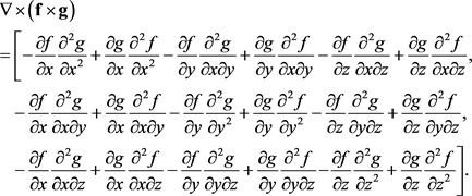
Third, the component definition of the cross product of two gradients and (37) yields

(52)

We then find the following definition of the curl of the cross product of and

(53)

Usage of the harmonicity conditions for f and g

(54)

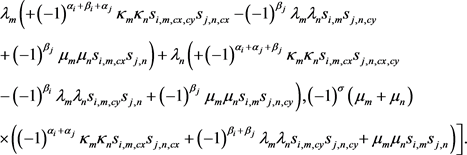
results in the component definition of the curl of the cross product of two harmonic gradients and:

(55)

Substitution of the theoretical DSK structures and in (55) and simplification by (12), (15) with, (15), and (12) with returns

(56)

Eventually, we add to (56) and subtract from (56) the relevant directional derivatives of (45) to get

(57)

The curl of the cross product of the DVK structures in the component form (56) is expanded in terms of the DSD structures (30). The curl of the cross product of the DVK structures in the vector form (57) is expressed via the commutator of the directional derivatives of the DVK structures (48).

Fourth, solving (51) with respect to the anticommutator yields

(58)

So, the scalar potential of the Helmholtz decomposition (58) of the anticommutator field is the dot product of the m-DVK and n-DVK structures.

Finding the commutator from (57) gives

(59)

Thus, the vector potential of the Helmholtz decomposition (59) of the commutator field is equal to the negative cross product of the m-DVK and n-DVK structures.

Multiplication of the Helmholtz decompositions (58)-(59) by 1/2, addition, and subtraction produce

(60)

(61)

where

(62)

is a scalar potential and

(63)

is a vector potential of the Helmholtz decompositions (60)-(61) of the fields of the directional derivatives of the m-DVK and n-DVK structures.

It was also verified that the theoretical expansions in terms of the DVD and DSD structures (43), (45), (48), (50)-(51), (56)-(61) completely describe the correspondent expansions via the experimental DVD and DSD structures.

6. The Stokes Field

Internal waves of a Newtonian fluid with a constant density and a constant kinematic viscosity in a field of gravity are governed by the momentum conservation law

(64)

and the mass conservation law [3]

(65)

The quasi-scalar Dirichlet problem for the Navier-Stokes Equations (64)-(65) may be set for the z-component of the velocity field on the upper and lower boundaries of the upper domain U (6)

(66)

and the upper and lower boundaries of the lower domain L (8), e.g. [1] [2],

(67)

An admissible decomposition of the boundary function in DSK boundary structures will be considered in Section 6 later. The conditions at infinity are satisfied due to (7) and (9). Configuration of the upper and lower domains of internal waves, which are generated through the boundary conditions (66)-(67) by surface waves propagating in a generation domain, is shown in Figure 2.

From viewpoint of the Fundamental Theorem of Vector Analysis [4] the Dirichlet problem (66)-(67) for the Navier-Stokes Equations (64)-(65) may be treated as a construction of the Helmholtz decomposition for the Archimedean field, the Stokes field, and the Navier field:

(68)

(69)

(70)

The Archimedean, Stokes, and Navier fields are decomposed using the correspondent scalar potentials and as follows:

(71)

where stands in fluid dynamics for the hydrostatic pressure, for the kinematic pressure, and for the dynamic pressure.

Summation of (68)-(71) yields the Helmholtz representation of the momentum conservation law (64)

(72)

where, which is termed in fluid dynamics a total pressure, is a scalar potential of the superposition of the Archimedean, Stokes, and Navier fields.

The problem of finding the scalar potential of the Archimedean field has a general solution [3]

(73)

where is a reference pressure of the Cauchy integral [5].

The problem of calculating the kinematic velocity field and the scalar potential of the Stokes field is equivalent to the following quasi-scalar Dirichlet problem for the Stokes equations:

(74)

It will be called afterwards the Stokes problem.

The problem of computing the scalar potential of the Navier field for the given field

(75)

will be later referred to as the Navier problem.

Decomposition of the Navier-Stokes problem (64)-(67) into the superposition of the Archimedean problem (68), (71), (73), the Stokes problem (69), (71), (74), and the Navier problem (70), (71), (75) is justified by the structure of the total pressure (72). From the mathematical standpoint, an exact solution of the Stokes problem (74) requires a balance of terms, which are linear in, but an exact solution of the Navier problem (75) necessitates a balance of terms, which are quadratic in. As to the fluid-dynamic viewpoint, the Navier problem models the inertial regime of intermittency of flows at high Reynolds numbers and the Stokes problem describes the viscous regime of generation/decay of flows at low Reynolds numbers.

To construct general solutions for the kinematic velocity and the kinematic pressure of the Stokes problem (74), we start from the following definitions of anormalized DSK structures:

(76)

where the DSK functions are given by (3) and functional amplitudes are wave parameters, which do not depend on (x, y, z, t).

Using a quadratic norm, which is given by a weight

(77)

the anormalized amplitudes are reduced to the normalized amplitudes of (1) by

(78)

because

(79)

Substitution of (78) in definitions (76) yields

(80)

Relationships between anormalized DVK structures and the normalized ones (20) are similar due to the scalar-vector structural invariance since

(81)

The general solution for the kinematic velocity is decomposed in four wave groups with M internal waves per group using the anormalized DVK structures in the following form:

(82)

In agreement with (81) and (80),

(83)

and the general solution in the normalized DVK structures after changing the order of summation reads

(84)

The velocity field (84) delivers the general solution of a direct problem of construction of the velocity field with given weights of quartets of the experimental DVK structures.

For an inverse problem of reconstruction of the velocity field from data of a laboratory experiment, a linear norm, which is set via a weight

(85)

may be used to transform the quartet weights into quartet probabilities

(86)

since

(87)

So, the general solution of the inverse problem may be written as follows:

(88)

where equiprobability of the experimental DVK structures, which are shown in Figure 1, is explained by quadrality of the theoretical DVK structures.

In agreement with the Cauchy integral, we construct the field of kinematic pressure via general terms in the following form:

(89)

Substitution of the temporal derivative (19) gives the general solution for of the direct problem

(90)

and the general solution for of the inverse problem

(91)

Substituting the velocity field and the pressure field in the Partial Differential Equations (PDEs) of the Stokes problem (74) and using the temporal derivative of the DVK structures (28), the Laplacian of the DVK structures (27), the gradient of the DSK structures (22), and the divergence of the DVK structures (23) yield that PDES of (74) are satisfied identically both for the direct solutions (84), (90) and the inverse solutions (88), (91).

To construct the DSK boundary structures, primarily, we set the DSK boundary functions for and as

(92)

So, the DSK boundary functions (92) are compatible with the DSK functions (3), where are wave numbers of boundary waves,

(93)

are the boundary Cartesian coordinates, are propagation velocities, and are initial coordinates of the boundary waves.

In accordance with (1), the DSK boundary structures are defined by

(94)

where functional amplitudes are normalized, i.e.

(95)

All boundary parameters do not depend on (x, y, z, t).

Eventually, we define the boundary function of (66)-(67) via the DSK boundary structures in the following form:

(96)

In agreement with (22), the z-component of the general solution (84) for the velocity field becomes

(97)

If and only if

(98)

then the dependent Cartesian coordinates, the scale multiplier in the z-direction, the theoretical DSK function, and the theoretical DSK structure are related with the correspondent boundary variables as follows:

(99)

In this case, the z-component of the velocity field (97) is reduced to the boundary function (96) and the Dirichlet boundary condition of the Stokes problem (74) is fulfilled exactly.

7. The Navier Field

A rectangular summation of all vector elements of a square matrix

(100)

with, which is represented by a double sum, may be always reduced to a triangular summation of diagonal terms and pairs of terms above and beneath the diagonal by the following formula:

(101)

Indeed, the triangular summation is also valid for a square matrix with scalar elements.

Primarily, we expand the velocity field (84) into J wave groups

(102)

where the velocity fields and of the ith and jth wave groups, respectively, are

(103)

Substitution of expansions (102) in the Navier field (70), reduction by the rectangular summation, and transformation by the triangular summation (101) in wave groups with substitutions yields

(104)

The directional derivative that describes propagation of the ith wave group in view of (103) may be written using the rectangular and triangular summations through the DVK structures as follows:

(105)

Likewise, the directional derivatives that express interaction of the ith and jth wave groups via the DVK structures become

(106)

Secondly, we start potentialization of the directional derivative (105) substituting the following Helmholtz decompositions:

(107)

which are derived from (60) and (61) by substitutions and. The result is

(108)

To proceed with potentialization of the directional derivatives (106), the necessary Helmholtz decompositions of the relevant directional derivatives

(109)

are obtained by substituting in (60) and (61) and. Substitution of (109) in (106) gives

(110)

We then use (108) and (110) to get from (104) the Navier field in the potentialized form

(111)

Thirdly, the Navier field is reduced using conversion of the triangular summation in wave groups into the rectangular summation as

(112)

By decomposition of rectangular sums into products of sums and conversion of the triangular summation with respect to internal waves into the rectangular summation, is transformed into the following completely rectangular form:

(113)

Comparison of (113) with the definition of yields the dynamic pressure of the direct problem

(114)

and, together with (86), the dynamic pressure of the inverse problem

(115)

Using connection (38) between the Laplacian of the DSD structure and the scalar product of the DVK structures, we get

(116)

Equation (116) demonstrates a mathematical meaning of the dynamic pressure that is a source of the stationary diffusion of the weighted superposition of all DSD structures with a diffusion coefficient.

Potentialization of the Navier field is possible since internal vortex forces, which are described by the vector potentials of the Helmholtz decompositions (107) and (109), counterbalance each other, in agreement with Newton’s third law. On the contrary, external potential forces, which are expressed via the scalar potentials of (107) and (109), superpose together to form the gradient of the dynamic pressure, in accord with Newton’s second law.

8. Discussion

Transformation of the Navier field (113) into the following product of two double sums

(117)

shows that the dynamic pressure and the kinetic energy have the same magnitude as since in agreement with (71), (113), (114), (117), (22), and (12), an orthogonal decomposition of in the DSD structures becomes

(118)

A non-orthogonal distribution of the kinetic energy between the wave groups, which is obtained using the triangular summation with respect to wave groups, has the following form:

(119)

where is the kinetic energy of propagation of the ith wave group and is the kinetic energy of interaction between the ith and jth wave groups.

We then find a non-orthogonal distribution of the propagation energy between internal waves, making the triangular summation (101) in regard to internal waves, to get

(120)

where is the kinetic energy of propagation of the mth internal wave of the ith wave group and is the kinetic energy of interaction between the mth and nth internal waves of the ith wave group.

Similarly, the triangular summation of gives the following non-orthogonal distribution of the interaction energy between internal waves:

(121)

where is the kinetic energy of interaction between the mth waves of the ith and jth groups, is the kinetic energy of interaction between the mth wave of the ith group and the nth wave of the jth group, and is the kinetic energy of interaction between the nth wave of the ith group and the mth wave of the jth group.

Substituting the computed general terms (120)-(121) in (119), we conclude with the non-orthogonal decomposition of the kinetic energy

(122)

into the following seven constituents. First, the cumulative kinetic energy of propagation of J wave groups

(123)

Second, the cumulative kinetic energy of interaction between J wave groups

(124)

Third, the cumulative kinetic energy of propagation of the mth internal waves of J wave groups

(125)

Fourth, the cumulative kinetic energy of interaction between the mth and nth internal waves of J wave groups

(126)

Fifth, the cumulative kinetic energy of interaction between the mth internal waves for J distinct wave groups

(127)

Sixth, the cumulative kinetic energy of interaction between the mth wave of the ith group and the nth wave of the jth group for J distinct wave groups

(128)

Seventh, the cumulative kinetic energy of interaction between the nth wave of the ith group and the mth wave of the jth group for J distinct wave groups

(129)

The kinetic energy (118) and its constituents (125)-(129) are compared in Figure 3 and Figure 4 for three wave groups with two internal waves each at for and the following wave parameters:

(130)

The kinetic energy and the cumulative kinetic energy of propagation demonstrate the pulsatory topology since the exact, nonlinear, three-dimensional (3-D), periodic solutions of the Navier-Stokes Equations (64)-(65) are strictly positive for all (x, y, z, t), and may be called exponential pulsons of elevation. Topology of the exponential pulsons is the same as of the solitons on shallow water, the solitary waves on shallow water with uniform and linear vorticity [6] [7], the solitary waves generated by crossed electric and magnetic fields [8], and the pulsatory waves of the Korteweg-de Vries equation [9],

which are exact nonlinear solutions for propagation and conservative interaction of aperiodic one-dimensional (1-D) waves. In view of (118), the corresponding solutions for the dynamic pressure and its propagation constituent are given by exponential pulsons of depression since they are strictly negative for all (x, y, z, t).

The cumulative kinetic energies of interaction exhibit the oscillatory topology since the exact, nonlinear, 3-D, periodic solutions of the Navier-Stokes Equations (64)-(65) alternate signs for various (x, y, z, t) and might be called exponential oscillons. Topology of the exponential oscillons is the same as of the solitons on deep water [10], which are exact nonlinear solutions for propagation and conservative interaction of aperiodic 1-D waves. The related solutions for the interactive constituents of the dynamic pressure and the total pressure are represented by the exponential oscillons, as well. Animations of visualizing propagation and conservative interaction of the exponential pulsons and oscillons, which are various superpositions of the time-dependent, 3-D, periodic DSD structures (29)-(30), confirm conservation of both the pulsatory and oscillatory topologies for all (x, y, z, t).

9. Conclusions

The most interesting properties of the scalar and vector kinematic structures that are studied in Section 2 and Section 3, respectively, are the scalar and vector structural oscillations, the scalar-vector duality, the quadrality of the theoretical DSK and DVK structures, and the equiprobability of the experimental DSK and DVK structures. The differentiation diagram in Figure 1 is actually an image of a mathematical two-dimensional dice, where all vertices have exactly the same probability despite the various scales of differentiation in the x- and y-directions.

The success of the scalar and vector dynamic structures treated in Section 4 and Section 5, correspondingly, is explained by their exact similarity to the Navier-Stokes Equations (64)-(65) as the momentum conservation law (64) represents a superposition of kinematic terms and dynamic terms with an algebraic nonlinearity. Further attractive features of the DSD and DVD structures are the absence of a formal restriction on the functional amplitudes, the structural amplitudes, and the quartet weights and the global convergence the DSD and DVD structures for all (x, y, z, t). For instance, the general solution of fluid dynamics in the Boussinesq-Rayleigh series converges only locally and the radius of convergence diminishes with the Reynolds number [11].

The large number of the experimental DSD and DVD structures, 16 and 32, respectively, is required for completeness of the expansions of the directional derivative of the global velocity and the gradient of the total pressure since otherwise the vortical forces produced by the vector potential (63) of the Helmholtz decomposition may not compensate each other. Therefore, the experimental and theoretical programming in Maple that facilitates computation and verification of the numerous large arrays of scalar and vector terms is essential for development of the general solution for J wave groups with M internal waves. Since the exact general solution is not affected by viscous dissipation it may serve as the 3-D model of conservative propagation and interaction of kinetic energy of internal waves in ocean and atmosphere via the exponential oscillons and pulsons visualized in Figure 3 and Figure 4.

Research in the functional amplitudes of the DSK structures started in [2] has revealed existence of three types of wave lattices: 1) slanted up and down, 2) stepped up and down with rectangular steps, and 3) stepped up and down with smooth steps. It is interesting to explore the effect of the wave parameters on the Eulerian and Lagrangian properties of the DSD structures, as well. By the well-known conjecture [12], chaos of physical systems is explained by superposing of a large number of deterministic solutions. Therefore, it also looks appealing to study stochastic properties of the general solution.

Acknowledgements

The support of CAAM is gratefully acknowledged. The author would like to thank reviewers and editor for valuable comments which have significantly improved the paper.