


Abstract
Several solar system moons harbor subsurface water oceans; extreme internal heating or solar irradiation can form magma oceans in terrestrial bodies. Tidal forces drive ocean currents, producing tidal heating that affects the thermal−orbital evolution of these worlds. If the outermost layers (ocean and overlying shell) are thin, tidal dynamics can be described using thin-shell theory. Previous work assumed that the ocean and shell's thickness and density are uniform. We present a formulation of thin-shell dynamics that relaxes these assumptions and apply it to several cases of interest. The tidal response of unstratified oceans of constant thickness is given by surface gravity and Rossby waves, which can resonate with the tidal force. The oceans of the outer solar system are too thick for gravity wave resonances, but high-amplitude Rossby waves can be excited in moons with high orbital obliquity. We find that meridional ocean thickness variations hinder the excitation of Rossby waves, decreasing tidal dissipation and increasing the inclination damping timescale, which allows us to reconcile the present inclination of the Moon with the existence of a past long-lived magma ocean and to explain the inclination of Titan and Callisto without invoking a recent excitation. Stratified oceans can support internal gravity waves. We show that dissipation due to internal waves can exceed that resulting from surface gravity waves. For Enceladus, it can be close to the moon's thermal output, even if the ocean is weakly stratified. Shear due to internal waves can result in Kelvin–Helmholtz instabilities and induce ocean mixing.
Export citation and abstract BibTeX RIS

Original content from this work may be used under the terms of the Creative Commons Attribution 4.0 licence. Any further distribution of this work must maintain attribution to the author(s) and the title of the work, journal citation and DOI.
1. Introduction
The list of known planets and moons with water oceans has grown from just Earth to also including some of the icy moons of the outer solar system. There is evidence that the Jovian moons Europa, Ganymede, and Callisto and the Saturnian moons Mimas, Enceladus, Dione, and Titan harbor subsurface oceans (Khurana et al. 1998; Kivelson et al. 2002; Iess et al. 2012; Tajeddine et al. 2014; Saur et al. 2015; Beuthe et al. 2016; Thomas et al. 2016; Rhoden & Walker 2022), and subsurface oceans are also suspected for some of the ice giants' moons (e.g., Hussmann et al. 2006; Nimmo & Spencer 2015; Bierson & Nimmo 2022). Rocky planets and moons are expected to have magma oceans during the early stages of their evolution (Elkins-Tanton 2012); vigorous tides might melt a body's mantle, as debated for Io (Khurana et al. 2011; Blöcker et al. 2018); and close-in exoplanets experiencing high solar irradiation or extreme stellar tides are also expected to have magma oceans (e.g., Chao et al. 2021). Many of these worlds can be labeled as thin-shell worlds. Their outermost layers, ocean and solid shell, are thin compared with the body's radius. Tidal forces periodically deform the outer shells of thin-shell worlds and excite tidal waves in their subsurface oceans. These processes are not adiabatic; part of the tidal energy is transformed into heat—a phenomenon known as tidal heating—which in turn plays a central role in the thermal and orbital evolution of these worlds (e.g., Darwin 1880; Kaula 1964; Peale et al. 1979; Yoder & Peale 1981; Ojakangas & Stevenson 1986; Hussmann et al. 2002; Tyler 2008; Chen et al. 2014).
Initially, work on the tidal dynamics of ocean worlds focused on body tides and ignored ocean dynamics (e.g., Cassen et al. 1979; Ross & Schubert 1987; Ojakangas & Stevenson 1989; Hussmann et al. 2002; Jara-Orué & Vermeersen 2011). But in the past two decades, several authors have considered the role of ocean tides in the tidal response of ocean worlds (Sagan & Dermott 1982; Dermott & Sagan 1995; Tyler 2008, 2009, 2011, 2021; Chen et al. 2014; Matsuyama 2014; Kamata et al. 2015; Beuthe 2016; Hay & Matsuyama 2017; Auclair-Desrotour et al. 2018; Matsuyama et al. 2018; Hay & Matsuyama 2019; Rekier et al. 2019; Rovira-Navarro et al. 2019, 2020). With few exceptions (Rekier et al. 2019; Rovira-Navarro et al. 2019), ocean dynamics have been investigated in the context of thin-shell dynamics. The equations used by Laplace to study Earth's oceans tide (Laplace 1798), known as the Laplace tidal equations (LTEs), have been the go-to tool to study extraterrestrial tides. The LTEs have been extended to account for the effects of an overlying solid shell (Beuthe 2016; Matsuyama et al. 2018). Nevertheless, previous work on ocean tides has often relied on the assumptions that (1) the thicknesses of the ocean and solid shell are spatially uniform and (2) the ocean's density is uniform, both of which are not always justified.
Ocean thickness variations can be the result of ocean basal topography or shell thickness variations. Shell thickness variations can arise owing to geographical variations of tidal heating and solar radiation (Ojakangas & Stevenson 1989) and to heat transport within the ocean (e.g., Soderlund 2019). Gravity and shape data can be used to infer shell thickness variations. Ice-shell thickness variations are expected to be less than 7 km in Europa and 12 km in Titan (Nimmo et al. 2007; Lefevre et al. 2014). In Enceladus, ice-shell thickness variations are more dramatic; the shell thickness varies from 30 km at the equator to just 5 km at the poles (Beuthe et al. 2016; Čadek et al. 2016; Hemingway & Mittal 2019), making evident that assumption 1 is not valid. Basal topography is more difficult to constrain, but an irregular core has been proposed for Enceladus (McKinnon 2013). Beuthe (2018, 2019), Souček et al. (2019), and A et al. (2014) studied the tidal deformations of a variable-thickness ice shell but ignored ocean dynamics; on the other hand, Rovira-Navarro et al. (2020) considered the dynamics of an Enceladan ocean of variable thickness but assumed an ice shell of constant thickness. The coupled dynamic response of a variable-thickness ocean covered by a shell of variable thickness remains to be considered.
Assumption 2 has often been justified invoking that subsurface oceans are convecting. As opposed to Earth's oceans, whose surface is heated by solar irradiation, the main heat source of a subsurface ocean is basal heat, making them prone to convection and mixing (e.g., Soderlund et al. 2013; Soderlund 2019; Amit et al. 2020). Nevertheless, certain processes (e.g., melting, double diffusive convection, the thermodynamic properties of fresh water near its melting temperature) can lead to stratified subsurface oceans (Melosh et al. 2004; Vance & Brown 2005; Vance & Goodman 2009; Lobo et al. 2021; Zeng & Jansen 2021), questioning assumption 2. Tyler (2020, 2011) suggested that baroclinic tides in a stratified ocean could lead to significant tidal dissipation relying on a one-layer constant-density model with an effective depth representative of the ocean's stratification and ignoring the role of the overlying shell. A model that captures the baroclinic response of a subsurface ocean is still missing.
The objective of this paper is to relax assumptions 1 and 2, present a general method to study the tidal dynamics of thin-shell worlds, and apply it to several cases of interest. To this end, in the first part of the paper we will present a generalized formulation of thin-shell tidal dynamics for stratified oceans of variable thickness covered by solid shells of variable thickness (Section 2.1) and introduce a semianalytical method to solve the equation of motion for a general tidal forcing (Section 2.2). We will then focus on the tidal response of the moons of the solar system and consider the specific case of synchronous satellites with nonzero eccentricity and obliquity (Section 2.3).
In the second part of the paper (Section 3), we will apply the new method to various cases of interest. We will start by quickly reviewing the main characteristics of the tidal response of an unstratified ocean of constant thickness (Section 3.1). Afterward, we will consider the role that ocean thickness variations have in the tidal response of subsurface oceans (Section 3.2). We will consider how ocean thickness variations can alter the thermal and orbital evolution of moons with subsurface oceans, and we will examine how shell and ocean thickness variations affect the deformation of Enceladus's ice shell. In Section 3.3, we will consider the role of ocean stratification. We will examine under which conditions internal gravity waves can be excited in subsurface oceans of constant thickness and whether they can resonate with the tidal force. Finally, we will focus on Enceladus to assess whether internal waves can explain the moon's endogenic activity. The combined case of a stratified ocean of variable thickness is left for future work.
2. Thin-shell Dynamics
We consider a body whose outermost layers consist of an ocean, which might be stratified in layers of different densities, and a solid shell (Figure 1). The tidal response can be obtained using the mass and momentum conservation equations for both layers under appropriate boundary conditions. If the wavelength of the forcing is large compared with the thickness of each of the layers, the equations can be radially averaged and greatly simplified; the system is described by thin-shell dynamics. This is generally the case for the bodies under consideration; the tidal perturbation wavelength is approximately the body's radius, which is larger than the ocean and shell thicknesses (see Table 2).

Figure 1. A two-layer ocean overlaid by a solid shell of variable thickness. Dashed and solid lines correspond to the unperturbed and perturbed states, respectively.
Download figure:
Standard image High-resolution imageFor the ocean, the thin-shell approximation leads to the shallow-water equations (Vallis 2006). The radial velocity is assumed to be small compared with the horizontal velocity, making it possible to neglect terms associated with the vertical velocity in the momentum equations. The equations are further simplified by employing the traditional approximation, which consists in neglecting the locally horizontal component of the Coriolis force. When this is done, the radial momentum equation reduces to hydrostatic equilibrium—a concise review of this approximation and its limitations can be found in Gerkema et al. (2008).
For the solid shell, the high viscosity and the high speed of seismic waves compared with the tidal period allow to neglect the inertial terms of the momentum equations. In such a case, the theory of viscoelastic-gravitational deformations can be employed to obtain the deformation and stress of the shell (e.g., Jara-Orué & Vermeersen 2011; Sabadini et al. 2016). As for the ocean, if the shell thickness is much smaller than the radius of the body, the equation of motion can be reduced from 3D to 2D (Beuthe 2008). As a rule of thumb, the thin-shell equations are valid for shell thickness to radius ratios up to ∼5%–10% (Beuthe 2018). This might not be the case for the smallest ocean worlds, such as Enceladus and Mimas, for which the ratio can exceed 10%, making this approximation more problematic for these bodies. Thin-shell equations for solid shells have been used in multiple geophysical applications, including lithospheric flexure (Beuthe 2008), and the tidal deformation of moons with subsurface oceans without (Beuthe 2015a, 2015b, 2018, 2019) and with ocean dynamics (Beuthe 2016). Results obtained using thin-shell equations show good agreement with those found using the 3D viscoelastic-gravitational equations of motion (Matsuyama et al. 2018). Recently, Beuthe (2018, 2019) extended the thin-shell equations to shells of variable thickness, to study the tidal response of moons with solid shells of variable thickness, but neglected ocean dynamics.
Below we will present the thin-shell equations that describe the coupled tidal dynamics of ocean and shell. Compared with previous work, the equations presented below permit thickness variations in both ocean and solid shell and are valid if the ocean is stratified. In Section 2.1 we will present the equations of motion; afterward, we will describe a spectral method to solve them (Section 2.2); and finally, we will focus on the form that the forcing takes for a synchronous body in an inclined and eccentric orbit (Section 2.3).
2.1. Equations of Motion
We consider an ocean of total thickness Hocean that is partitioned into N layers of densities ρi , where i stands for the index of the layer. Additionally, we consider that the ocean might be covered by a solid shell of thickness Hshell. A sketch of the system for a two-layer ocean is shown in Figure 1. The thickness of each layer is given by hi , which we further split into its unperturbed average thickness Hi and a perturbation,

For each layer, we can write the mass conservation equation as

where s i is the momentum flux, defined as

and u is the tangential flow velocity.
Following the thin-shell approximation, we consider that the radial momentum equation is simply given by hydrostatic equilibrium and obtain the momentum equation of each layer by vertically averaging the other components of the momentum equations

where pi is the pressure within the layer. D(hi , s i ) is a function that parameterizes dissipation within the layer, ϕ is the gravitational potential, 1r is the radial unit vector, and f is the Coriolis parameter

with θ being the colatitude and Ω the body's rotational frequency. We have assumed that perturbations are small and linearized the equations of motion. This makes the problem analytically tractable and allows us to obtain wave solutions, but it implies that nonlinear effects that can lead to instabilities and turbulence are ignored (see discussion in Section 3.3).
The pressure within each layer can be obtained using hydrostatic balance
where q is the dynamic pressure exerted by the solid shell on the ocean, η0 is the displacement of the solid surface, and z is measured from the surface and is positive upward. From the previous expression it is evident that even though there might be no perturbations (η = 0), a pressure gradient driving ocean flows can arise if layers are not constant in thickness. We consider that this is compensated by a transport mechanism that maintains the stratification structure. As we use the linearized LTEs, we assume that this flow does not interact with tidally driven currents and only consider flows induced by gradients in η.
The dissipative function D can take different forms depending on the leading dissipation mechanism (e.g., Hay & Matsuyama 2017)

The first term is a linear dissipation term; ocean dissipation is proportional to the velocity via the Rayleigh parameter α. It is akin to the viscous term of a damped oscillator and considers that dissipative processes have a characteristic timescale equal to the inverse of the Rayleigh parameter for all spatial and temporal scales. The second term is proportional to the square of the velocity via the bottom drag coefficient cD and is often used to account for dissipation in fluid-solid boundaries due to friction. The third term is a diffusive term; ν can be either the dynamic or an eddy viscosity. On Earth tidal dissipation occurs mostly as a result of bottom drag and is well captured by the second term. There exist empirical constraints on the value of cD from Earth studies; because of this, several studies of tides in icy moons have considered bottom drag as the main dissipative source (Chen & Nimmo 2016; Hay & Matsuyama 2017, 2019). However, this has the disadvantage of introducing a nonlinear term in the equations of motion and might not capture other dissipative processes at play in subsurface oceans. For these reasons many studies have used a linear drag term (Tyler 2011, 2014; Matsuyama 2014; Beuthe 2016; Matsuyama et al. 2018; Hay et al. 2020; Rovira-Navarro et al. 2020). We will assume a linear dissipation term that can account for different dissipative processes and vary α over various orders of magnitude. It is useful to note that scaling analysis can be used to obtain an effective Rayleigh coefficient α for a given value of bottom drag coefficient cD . Matsuyama et al. (2018) showed α to be between 10−5 and 10−11 s−1 for Europa and Enceladus.
Plugging Equation (6) into Equation (4) and considering Rayleigh dissipation, we find the linearized thin-shell equations

Here ci
2 is the square of the surface wave speed  ; we will assume that displacements η are smaller than the layer thickness and hence use
  .
.
Viscous processes within the ocean cause energy dissipation. In our approach, dissipative processes are parameterized via the Rayleigh coefficient α. The average amount of tidal dissipation in layer i for a period T is given by

Alternatively, the total tidal dissipation can be computed by considering the work done by the tidal force in the ocean (Chen et al. 2014),

The pressure term q couples ocean and shell dynamics. q is related to the displacement of the ocean surface, η1. As mentioned above, we use thin-shell theory for shells of variable thickness (Beuthe 2008, 2018). For shells of constant thickness, the pressure load results in a normal load at the bottom of the shell. In contrast, for shells of variable thickness a lateral load proportional to the slope of the shell−ocean interface also arises. As we consider long-wavelength thickness variations, which are characterized by small slopes, we neglect this component and assume that the ocean pressure exerts only a normal load. We use the massless approach (Beuthe 2015a), which assumes that the density contrast between the ocean and solid shell is zero and adds the shell mass to the ocean. This implies that we neglect the gravitational perturbation that results from the ocean−shell density contrast, which is small owing to the small density contrast and hence results in a small error (e.g., 2% in the case of Enceladus; Beuthe 2018). The solid shell dynamics is then described by
F is an auxiliary variable called the stress function, and η0 is the radial surface displacement. From the thin-shell approximation it follows that the transverse displacement is constant within the shell, and hence η1 = η0.  and
and  are two differential operators defined in Appendix F. α(e) and D(b) are the inverse of the extensional rigidity and the bending rigidity:

Here ν is the Poisson ratio and μ0 is the vertically averaged shear modulus, or more generally the p = 0 moment of the shear modulus,
with h being the distance from a reference surface within the shell. Parameter μinv is given by

χ and ψ are two purely geometrical parameters given by

with δ = Hshell/R. Apart from ocean currents and shell deformations, the tidal potential also deforms the mantle. Additionally, the mantle deforms in response to the ocean load and shell pressure q. As we will see, the effects of a nonrigid mantle can be accounted for using the tidal, load, and pressure Love numbers of the mantle (Matsuyama 2014; Beuthe 2016; Matsuyama et al. 2018).
2.2. A Semianalytical Method to Solve the Thin-shell Equations
The tidal response is obtained by solving Equations (8) and (11b). We use a semianalytical method based on spherical harmonics. The method is similar to that previously used to solve the LTEs for oceans of constant thickness and density (Longuet-Higgins 1968; Tyler 2008; Chen et al. 2014; Matsuyama 2014; Beuthe 2016) but is extended to accommodate both ocean and solid shell thickness variations, as well as ocean stratification.
We first split the gravitational potential into two components, one corresponding to the forcing tidal potential ϕT, and the other, ϕSG, arising from the deformation of the body and its self-gravity. We also rewrite the forcing term using

where ηT is the displacement of the ocean surface if ocean dynamics, self-gravity, and the presence of a shell are ignored. We decompose s i using a Helmholtz decomposition:

Using these definitions and taking ∇ · and 1r · ∇ × of Equation (8b), Equation (8) can be rewritten in terms of Φi and Ψi instead of s i (see Appendix A).
The resulting equations are solved in the spectral domain using spherical harmonics. The forcing term ηT is decomposed as

where ω is the frequency of the forcing and Yl m is a spherical harmonic of degree l and order m,
Pl,m are associated Legendre functions (e.g., Ivers & Phillips 2008; Arfken et al. 2013).
The solution is similarly expanded as
We split the parameters ci 2, Hshell, χ, (ψ χ α(e)), and (ψ χ D(b)) into a uniform and a variable component:
As lateral variations must be real, we have that if there are sectoral or tesseral variations (m ≠ 0), the expansion coefficients Al,m
must satisfy  , where * indicates the complex conjugate. Similarly, the Coriolis term—Equation (5)—can be written using spherical harmonics as

The gravitational potential arising from the deformation of the body (ϕSG) consists of a component resulting from the deformation of the outer layers (ϕL) and a component arising as a result of the deformation of the mantle. If the mantle is spherically symmetric and we use the thin-shell approximation, ϕSG can be written in terms of Love numbers as (Beuthe 2016)

Here kl
T, kl
L, kl
P are the gravitational tidal, load, and pressure Love numbers, respectively.  and
and  are the load and pressure potentials, which, assuming that density changes within the ocean are small Δρ/ρ1 ≪ 1, are given by
Here ρb is the bulk density of the body and ηl,m is the difference between the displacement of the top and the bottom of the ocean η1,l,m − ηN+1,l,m . The deformation of the bottom of the ocean is similarly given by

where hl T, hl L, hl P are the radial Love numbers. If the mantle is rigid, the Love numbers are 0; Appendix D provides analytical expressions of the Love numbers for a homogeneous mantle. Finally, it is useful to nondimensionalize the equations of motion. We use the definitions
with  and
and  .
.
Using Equations (20) and (21) and projecting Equations (11b) and (A1) onto spherical harmonics employing the properties listed in Appendix G, we can get an algebraic set of differential equations. First, from mass conservation in the ocean (Equation (A1a)), we relate  and
and  as
as

The previous expression can be used recursively to obtain  ,
,

Using Equations (23), (25), and (27), we write Equations (11b), (A1b), and (A1c) as

The operators  ,
,  ,
,  ,
,  , and
, and  are given in Appendix F, and υT, υL and υP are a set of coefficients related to the deformation of the mantle:
The main nondimensional parameters controlling the response of the moon are given in Table 1.  is the nondimensional forcing frequency.
  is the inverse of the characteristic ocean damping timescale; a high value indicates an overdamped system. The Lamb parameter
  is given by the ratio between the velocity at which a perturbation of frequency Ω and wavelength R propagates and the surface wave speed in a shell-free ocean. When
  , the terms on the left-hand side of Equation (8b) are much smaller than those on the right-hand side. Ocean dynamics is then negligible, and the ocean follows the equilibrium tide, which for a nongravitating shell-free body is simply given by
  . For synchronous satellites experiencing tides
  , and a look at Table 2 shows that the Lamb parameter is small for all bodies, indicating that surface waves do not play a significant role in their response to planet tides. This is not the case for tides raised by other moons in the system, for which the forcing frequency
  might be much higher than 1 and hence
  might not hold (Hay et al. 2020, 2022). The solid shell adds two additional nondimensional parameters: γ and
  . γ is the effective rigidity and indicates the importance of the shell on the tidal response. In bodies with a high effective rigidity (hard-shell bodies) the shell hinders ocean surface displacements—e.g., the amplitude of the equilibrium tide is reduced. In contrast, in bodies with low effective rigidity (soft-shell bodies) the shell does not hinder ocean surface displacements—the equilibrium tide is barely affected by the presence of the shell (Beuthe 2018; Matsuyama et al. 2018). From Table 2, we see that small bodies generally behave as hard-shell bodies and bigger ones as soft-shell bodies.
  is related to the importance of bending effects. The role of bending effects depends on the wavelength (see Equation (B2)); bending effects become more relevant as the wavelength decreases and start to become dominant when
  .
.  is small in all cases, indicating that bending effects are small for the long wavelengths characteristic of tides. ξ encapsulates the importance of ocean loading and ocean self-gravitation, if self-gravitation is ignored, ξ = 0. The amplitude of mantle deformations depends on the mantle's effecftive rigidity
  . As shown in Appendix D, the Love numbers of the mantle depend on this parameter as
  . The effective rigidity
  is generally large for the bodies considered here, which implies that the Love numbers and hence υ are small. Because of this, in what follows we will neglect mantle deformations.
Table 1. List of the Main Nondimensional Parameters Governing Tidal Dynamics
| Uniform Density and Thickness | |||
|---|---|---|---|
| Name | Symbol | Definition | Meaning |
| Nondimensional frequency |

|

| Ratio of forcing to rotating frequencies |
| Nondimensional damping frequency |

|

| Relevance of ocean dissipation processes |
| Ocean loading coefficient | ξ |

| Relevance of ocean loading and self-gravity |
| Lamb parameter |
|

| Relevance of surface gravity waves |
| Effective rigidity | γ |

| Relevance of the solid shell |
| Effective bending rigidity |

|

| Relevance of bending effects |
| Mantle effective rigidity |

|

| Role of mantle deformation |
| Variable Density | |||
| Relative layer thickness |

|

| Layer-to-total ocean thickness ratio |
| Density ratio | ri |

| Density contrast within the ocean |
| Variable Thickness | |||
| Relative ocean thickness variations |

|

| Amplitude of ocean thickness variations |
| Relative ice thickness variations |

|

| Amplitude of shell thickness variations |
Download table as: ASCIITypeset image
Table 2. Physical Parameters of a Selection of Tidally Active Bodies of the Solar System
| Moon | Io | Europa | Ganymede | Callisto | Mimas | Enceladus | Dione | Titan | Triton | |
|---|---|---|---|---|---|---|---|---|---|---|
| Radius (km) | 1737.4 | 1821.5 | 1560.8 | 2631.2 | 2410.3 | 198.2 | 252.1 | 561.7 | 2574.7 | 1353.4 |
| Mass (1022 kg) | 7.3 | 8.9 | 4.8 | 14.8 | 10.8 | 0.0037 | 0.011 | 0.11 | 13.5 | 2.1 |
| Average density (103 kg m−3) | 3.34 | 3.53 | 3.01 | 1.94 | 1.84 | 1.15 | 1.61 | 1.48 | 1.88 | 2.06 |
| Surface gravity (m s−2) | 1.62 | 1.80 | 1.32 | 1.43 | 1.25 | 0.064 | 0.11 | 0.23 | 1.35 | 0.78 |
| Shell thickness (km) | 50 | 30 | 30 | 125 | 115 | 28 | 23 | 99 | 100 | 150 |
| Ocean thickness (km) | 50 | 50 | 100 | 150 | 80 | 44 | 38 | 65 | 255 | 150 |
| Ocean thickness variations (km) | ⋯ | ⋯ | 7 | ⋯ | ⋯ | ⋯ | 22 | ⋯ | 12 | ⋯ |
| Tidal period (days) | 27.32 | 1.77 | 3.55 | 7.16 | 16.69 | 0.94 | 1.37 | 2.74 | 15.95 | 5.88 |
| Eccentricity (10−3) | 55.4 | 4.1 | 9.4 | 1.3 | 7.4 | 19.6 | 4.7 | 2.2 | 28.8 | ⋯ |
| Inclination (deg) | 5.16 | 0.036 | 0.466 | 0.177 | 0.192 | 1.57 | 0.003 | 0.028 | 0.306 | 156.87 |
| Obliquity (deg) | 6.68 | 0.0021 | 0.053 | 0.033 | 0.24 | 0.041 | 0.00045 | 0.0020 | 0.32 | 0.35 |
| Lamb parameter () | 7.2 × 10⁻³ | 6.2 × 10⁻² | 7.8 × 10⁻³ | 3.3 × 10⁻³ | 1.1 × 10⁻³ | 8.3 × 10⁻² | 4.2 × 10⁻² | 1.5 × 10⁻² | 4.0 × 10⁻⁴ | 2.4 × 10⁻³ |
| Effective rigidity (γ) | 6.2 × 10⁻¹ | 3.1 × 10⁻¹ | 8.2 × 10⁻² | 1.1 × 10⁻¹ | 1.4 × 10⁻¹ | 9.67 × 10 | 2.8 × 10 | 1.2 × 10 | 9.8 × 10⁻² | 9.2 × 10⁻¹ |
Bending ( ) ) | 7.7 × 10⁻⁵ | 2.5 × 10⁻⁵ | 3.45 × 10⁻⁵ | 2.1 × 10⁻⁴ | 2.1 × 10⁻⁴ | 1.8×10⁻³ | 7.8 × 10⁻⁴ | 2.9 × 10⁻³ | 1.4 × 10⁻⁴ | 1.1 × 10⁻³ |
| Amp. Equation eccentricity tide (m) | 2.3 | 40.9 | 23.3 | 2.2 | 2.1 | 229 | 23.7 | 6.8 | 9.4 | 0 |
| Amp. Equation obliquity tide (m) | 2.21 | 0.17 | 1.05 | 0.04 | 0.54 | 3.83 | 0.018 | 0.05 | 0.83 | 3.2 |
| Surface heat flux (W m−2) | ⋯ | 2.24 | 0.02 | ⋯ | ⋯ | ⋯ | 0.02–0.04 | ⋯ | 0.005 | ⋯ |
Note. Mass, radius, surface gravity, orbital period, eccentricity, and inclination are from NASA/JPL's Solar System Dynamics database (https://ssd.jpl.nasa.gov). Only the obliquity of the Moon and Titan correspond to measured values (Stiles et al. 2008; Lang 2011). For the remaining satellites the obliquity is computed by assuming that the satellite is in a Cassini state; see Chen et al. (2014) and Baland et al. (2016) for the icy moons and Baland et al. (2012) for Io. Representative shell and ocean thickness values: Io (Jaeger et al. 2003; Khurana et al. 2011); Europa (Anderson et al. 1998; Hussmann et al. 2002); Ganymede (Kivelson et al. 2002; Vance et al. 2018); Callisto and Titan (Vance et al. 2018); Enceladus and Dione (Beuthe et al. 2016); Mimas (Rhoden & Walker 2022); Triton (Nimmo & Spencer 2015). For the Moon, ocean thickness, shell thickness, and Lamb parameter are representative of values attained during the freezing process (Chen & Nimmo 2016). Ocean thickness variations for Europa, Enceladus, and Titan are from Nimmo et al. (2007), Beuthe et al. (2016), and Lefevre et al. (2014). Parameters , γ, and  are obtained assuming a Young modulus of 8.8 and 170 GPa for ice and rock, respectively, and a Poisson ratioof ν = 0.33. For Io the heat flux is estimated from astrometric measurements (Lainey et al. 2009); for Enceladus, it is obtained from Cassini's infrared observations of the south pole (Howett et al. 2011) and heat flux estimates obtained assuming that the moon is in thermal equilibrium (Hemingway et al. 2018); for Europa, it is estimated assuming that Europa is in thermal equilibrium (Hussmann et al. 2002); and for Titan, it is inferred from topography (Nimmo & Bills 2010).
Download table as: ASCIITypeset image
Lateral ocean or shell thickness variations add new nondimensional parameters:  , which depends on ocean thickness variations, and
  and
and  , which follow from shell thickness variations. Moreover, each ocean density interface adds two new nondimensional parameters: the density ratio between the two layers r, and the ratio between the thickness of the new two layers resulting from the new density interface,
  . As we will see, these two parameters control the excitation of internal waves.
We can get some insight into the problem by examining Equation (29d). The extra terms that arise from thickness variations and stratification are indicated. The terms with  are related to gravity waves in a shell-free ocean. Terms proportional to q arise from the presence of a shell, which, as we will later see, effectively increases the surface gravity wave speed. Terms with
  are the result of the Coriolis force. Without these terms, equations of different degree l would be decoupled. The terms containing
  are the result of ocean thickness variations. They couple equations of different degree and order even in the absence of rotation. Similarly, the terms
  and
and  arise as a result of lateral variations in shell properties. If there are only meridional thickness variations m1 = 0, equations with different orders are uncoupled as
  if m ≠ m2. If the ocean is unstratified (N = 1), it is of uniform thickness (
 for l ≠ 0), and we ignore the presence of a solid shell (γ = 0), we recover the classic LTEs used by Longuet-Higgins (1968) to study the response of a terrestrial global ocean and first employed by Tyler (2008, 2009) to study subsurface oceans. If we consider a spherically symmetric solid shell, we obtain the equation used in Beuthe (2016) (see Appendix B).
Equation (29d) constitutes a linear system of 2(1 + N)(L + 1)2 equations of the form

N is the number of layers, and L is the degree at which we cut the system of equations. A follows from Equations (29d), x is the vector containing the unknowns
and f is the forcing term
with fi,l,m,Φ and fi,l,m,Ψ being the forcing terms on the right-hand side of Equations (29a) and (29b). The superscript † indicates the transpose.
If we only consider a forcing of a given degree and order and restrict the problem to meridional ocean and shell thickness variations, the system reduces to 2(1 + N)(1 + L) equations. Moreover, if the shell is spherically symmetric, q and F can be written in terms of Φ and the system reduces to 2N(1 + L) (see Appendix B).
2.3. Tidal Response of a Synchronous Satellite
The approach presented above allows us to obtain the tidal response due to a general tidal perturbation. Here we will focus on the tides experienced by a synchronous satellite of nonzero eccentricity e and obliquity θi
. In this case  . The tidal potential has two components, the eccentricity (ϕe
) and the obliquity tide (ϕo
),
. The tidal potential has two components, the eccentricity (ϕe
) and the obliquity tide (ϕo
),

The tidal response of the ocean depends on the direction in which the tidal potential propagates. Because of this, the tidal potential is further split into westward- and eastward-propagating components (e.g., Chen et al. 2014; Beuthe et al. 2016),

The W and E superscripts indicate the westward and eastward components, respectively. The zonal component is a standing wave—it does not propagate in the longitudinal direction—however, splitting it into  and
and  components is convenient. The amplitude of each component of the tidal potential is given in Table 3. The solution is similarly expanded into westward- and eastward-propagating components


and the same for the remaining variables— ,
,  , and
, and  . Since the different variables should be real, it follows that
  , and similarly for the other fields.
Table 3. Amplitude of the Components of the Eccentricity and Obliquity Tides
| Tidal Component | Amplitude |
|---|---|

|

|

|

|

|

|

|

|

|

|

|

|
Download table as: ASCIITypeset image
Because the equations of motion have been linearized, we can compute the tidal response of the ocean for each component of the tide considering a unit forcing of  by solving Equation (29d) and then combining the solutions using the weights in Table 3. However, tidal dissipation is not linear (Equations (9) and (10)), and hence it should be generally computed once all the components of the tidal response have been obtained. Using the definition of
s
(Equation (3)), plugging Equations (35) and (36) into Equation (10), and using the orthogonality properties of vector spherical harmonics (Equation (G16b)), we find the total nondimensional energy dissipation
by solving Equation (29d) and then combining the solutions using the weights in Table 3. However, tidal dissipation is not linear (Equations (9) and (10)), and hence it should be generally computed once all the components of the tidal response have been obtained. Using the definition of
s
(Equation (3)), plugging Equations (35) and (36) into Equation (10), and using the orthogonality properties of vector spherical harmonics (Equation (G16b)), we find the total nondimensional energy dissipation
The dimensional tidal dissipation is given by

where the nondimensional term in parentheses accounts for the fact that while we force the problem with  , the magnitude of
  experienced by each satellite depends on its orbital frequency, radius, and surface gravity.
As noted above, examining Equation (37), we see that we cannot always separate the contribution of the different components of the tide to the energy budget. For example, if the eccentricity tide produces an m = 1 ocean tidal response ( , a term arising from the combination of this term with the obliquity tide (
 ) of amplitude
  appears. Nevertheless, in some special cases the contribution of tidal dissipation due to each component of the tide can be separated. If there are not lateral variations with odd order m, the contribution of eccentricity and obliquity tides can be separated. Similarly, if there are not lateral variations with even order m, the contribution of the m = 0 and m = 2 components can be separated. In the special case of only zonal variations, m = 0, the contribution of all tidal components to tidal dissipation can be separated. Below we will focus on this case and distinguish between tidal dissipation due to the eccentricity and the obliquity tide. Furthermore, to make the nondimensional tidal response independent of the eccentricity and obliquity of a specific body, we will obtain the tidal response for e = 1 and
  , which can be easily scaled to a particular body by multiplying by its eccentricity and obliquity.
3. Applications
After Section 2.1, we are now ready to study the tidal response of subsurface oceans. First, we succinctly summarize the main characteristics of the tidal response of an ocean of constant thickness and density, as it provides a reference with which the follow-up cases can be compared (Section 3.1). Afterward, we consider the tidal response of an unstratified ocean of variable thickness (Section 3.2), and finally we move to the case of a stratified ocean of constant thickness (Section 3.3).
3.1. Unstratified Ocean of Constant Thickness
The tidal response of unstratified oceans of constant thickness and density has been widely studied in the past decade (e.g., Tyler 2008, 2009, 2011; Chen et al. 2014; Matsuyama 2014; Beuthe 2016; Hay & Matsuyama 2017, 2019; Matsuyama et al. 2018). If the ocean is unstratified and both ocean and solid shell are of constant thickness, Equation (29d) reduces to

where Λl is a nondimensional shell spring constant proportional to the effective rigidity γ (Beuthe 2015a; see Appendix B).
Equation (39) can be cast into a matrix form and the solution obtained by inverting A. When A is close to singular, a resonance can occur. The frequencies  for which this happens are the eigenfrequencies of the system. The eigenfrequencies cannot be analytically obtained except if the moon is not rotating or the Coriolis terms are neglected (
 ), in which case A becomes diagonal. Note that in the nonrotating limit the rotational frequency of the body Ω is 0; instead of using the rotational frequency to nondimensionalize the equations of motion, we use the orbital frequency, ∣ω∣ (Equation (26)). Provided that the damping is small
  , the eigenfrequencies are

Using the previous expression, we can obtain the values of , for which the ocean resonates at the tidal frequency ( ),
),

which is equivalent to the expressions given in Beuthe (2015b) and Beuthe et al. (2016). These resonances correspond to surface gravity waves. Examining Equation (41), it becomes evident that the resonant increases with increasing degree or, equivalently, the resonant ocean thickness decreases with increasing degree. Moreover, we see that the presence of an elastic shell shifts the resonant ocean thickness toward lower values. From the values of and γ characteristic of the moons of the outer solar system (Table 2), we see that for all of them  , which implies that planet tides do not excite resonant surface gravity waves. Using
  and Equation (27), we find that in such cases the ocean surface displacement is well approximated by

the ocean surface follows the equilibrium tide.
As discussed above, the inclusion of rotation couples equations of different degrees l, changing the resonant frequencies of the system. Moreover, even though the tidal forcing is restricted to degree l = 2, modes containing shorter wavelengths can be excited, and, as opposed to the nonrotating case, the eigenfrequencies of the system depend on the order m and on whether the tidal wave propagates westward or eastward. Nevertheless, equatorial symmetric and antisymmetric modes remain decoupled. An equatorial symmetric forcing (e.g.,  ) results in a symmetric flow field (
![${{\boldsymbol{x}}}^{\mathrm{sym}}={[{\hat{{\rm{\Psi }}}}_{\mathrm{1,2}},{\hat{{\rm{\Phi }}}}_{\mathrm{2,2}},{\hat{{\rm{\Psi }}}}_{\mathrm{3,2}},{\hat{{\rm{\Phi }}}}_{\mathrm{4,2}}...]}^{\dagger }$](https://content.cld.iop.org/journals/2632-3338/4/2/23/revision1/psjacae9aieqn96.gif) ), while an antisymmetric forcing (e.g.,
), while an antisymmetric forcing (e.g.,  ) results in an antisymmetric flow field (
![${{\boldsymbol{x}}}^{\mathrm{asym}}={[{\hat{{\rm{\Psi }}}}_{\mathrm{1,1}},{\hat{{\rm{\Phi }}}}_{\mathrm{2,1}},{\hat{{\rm{\Psi }}}}_{\mathrm{3,1}},{\hat{{\rm{\Phi }}}}_{\mathrm{4,1}}...]}^{\dagger }$](https://content.cld.iop.org/journals/2632-3338/4/2/23/revision1/psjacae9aieqn98.gif) ).
).
The inclusion of rotation also introduces Rossby waves into the system. Tyler (2008) showed that the westward component of the obliquity tide ( ) can excite strong Rossby waves in thick subsurface oceans. The Rossby wave solution can be well approximated by cutting off Equation (39) at degree 2. Doing so, an analytical solution for Rossby waves can be obtained (Beuthe 2016),
If there is no energy dissipation ( ), the solution only contains the term
  and is equivalent to the solution derived in Tyler (2008). Moreover, as noted in Beuthe (2016), if
  and
and  , the flow velocity, ∇ × (Ψ1,1
1r
/H), is independent of ocean thickness and tidal dissipation increases linearly with ocean thickness.
, the flow velocity, ∇ × (Ψ1,1
1r
/H), is independent of ocean thickness and tidal dissipation increases linearly with ocean thickness.
The main characteristics of the tidal response of an unstratified ocean of constant thickness can be observed in Figure 2. For both eccentricity and obliquity tides, surface gravity waves occur at various values of Lamb parameter . Nevertheless, this occurs far from the region characteristic of the moons considered. Additionally, the excitation of Rossby waves is evident by an increase of tidal dissipation with decreasing for the obliquity tide. As expected from Equations (43), the amount of tidal dissipation due to Rossby waves depends on  (see Figure 2(d)). The lower
  is, the thicker the ocean for which tidal dissipation due to obliquity attains its maximum. This dependence disappears if tidal dissipation is modeled using nonlinear bottom drag rather than a Rayleigh dissipation coefficient, in which case dissipation becomes independent of ocean thickness (Hay & Matsuyama 2017, 2019). As opposed to surface gravity waves, Rossby waves can result in a significant amount of tidal dissipation for satellites with a high obliquity, most notably Triton (see Figure 2(e)), provided that the assumption of constant ocean thickness holds.

Figure 2. Nondimensional energy dissipation in an unstratified ocean of constant thickness due to the eccentricity and the obliquity tide as a function of Lamb parameter and effective rigidity γ (panels (a) and (b)) and the inverse of the damping timescale  (panels (c) and (d)). Bending effects and self-gravity are neglected and a cutoff degree of 30 is used. (e) Dimensional tidal dissipation is computed using the values given in Table 2 and assuming
  .
.
Download figure:
Standard image High-resolution image3.2. Unstratified Ocean of Variable Thickness
In this section we consider an ocean of uniform density but variable thickness covered by a shell of either constant or variable thickness. Rovira-Navarro et al. (2020) already investigated the tidal response of a global ocean of variable thickness using finite element modeling (FEM). However, the semianalytical method presented here allows a better exploration of the parameter space. In Appendix H, we show that, as expected, both methods lead to the same results.
We will first discuss how ocean thickness variations alter the eigenfrequencies of the ocean (Section 3.2.1). Afterward, we will discuss the important role of thickness variations for the excitation of Rossby waves and the damping of a moon's inclination (Section 3.2.2). Finally, we will consider the specific case of Enceladus in more detail (Section 3.2.3).
3.2.1. The Eigenmodes and Eigenfrequencies of an Ocean of Variable Thickness
As opposed to the case of an ocean and shell of constant thickness, if the ocean and shell are not spherically symmetric, the terms containing  ,
,  , and
, and  in Equation (29d) are not zero. The terms arising as a result of ocean thickness variations resemble the Coriolis term; they couple equations of different degrees. Moreover, while the Coriolis term does not couple equations of different orders, sectoral and tesseral thickness variations (mt
≠ 0) couple equations of different orders. An ocean with thickness variations of order mt
experiencing a forcing of order mf
responds with modes of orders mf
+ nmt
, with n being an integer, some of which might resonate with the tidal force.
in Equation (29d) are not zero. The terms arising as a result of ocean thickness variations resemble the Coriolis term; they couple equations of different degrees. Moreover, while the Coriolis term does not couple equations of different orders, sectoral and tesseral thickness variations (mt
≠ 0) couple equations of different orders. An ocean with thickness variations of order mt
experiencing a forcing of order mf
responds with modes of orders mf
+ nmt
, with n being an integer, some of which might resonate with the tidal force.
Even though sectoral and tesseral shell or ocean thickness variations are possible in subsurface oceans, we focus on meridional variations (mt
= 0, lt
≠ 0). This reduces the system of equations from 2(1 + L)2 to 2(1 + L). Contrary to the case of an ocean of uniform thickness, equatorially symmetric (
x
sym) and antisymmetric ocean modes (
x
asym) are not necessarily decoupled. Nevertheless, if ocean thickness variations are symmetric with respect to the equator,  when l and l2 have different parity and
  when both l and l2 have the same parity. This implies that if the ocean has symmetric ocean thickness variations, symmetric and antisymmetric modes are decoupled, as was the case for a constant-thickness ocean. In contrast, antisymmetric ocean thickness variations couple symmetric and antisymmetric modes, making it possible for a symmetric forcing to excite an antisymmetric ocean response and vice versa.
To illustrate the effects of ocean thickness, we consider long-wavelength ocean thickness variations of degree 2 and 3 ( or
or  ). An ocean with
  is symmetric with respect to the equator and thicker at the poles than at the equator, and one with
  is antisymmetric with respect to the equator and thicker at the north pole than at the south pole.
The effects of ocean thickness variations in the tidal response of a subsurface ocean are illustrated in Figure 3. As in Rovira-Navarro et al. (2020), we observe that degree 2 ocean thickness variations decrease  . Degree 3 ocean thickness variations do not alter the resonant ocean thickness for modes already excited in a constant-thickness ocean but introduce new modes, which appear as new bands of intense dissipation in Figures 3(c) and (d). These are antisymmetric modes excited by the symmetric eccentricity tide and symmetric modes excited by the antisymmetric obliquity tide.

Figure 3. Nondimensional energy dissipation in an unstratified ocean with degree 2 (panels (a) and (b)) and 3 (panels (c) and (d)) ocean thickness variations. Self-gravity is neglected, and a surface ocean is assumed,  ; we use
  . A cutoff degree of 30 is used. The case corresponding to an ocean of constant thickness (
 ) is indicated with a white dashed horizontal line.
Download figure:
Standard image High-resolution imageThe most dramatic effect is the change of tidal dissipation due to obliquity tides for low values of Lamb parameter (see Figures 3(b) and (d)). Ocean thickness variations inhibit the excitation of Rossby waves. This is evident as a decrease of energy dissipation for thick oceans ( ≪ 1) as ocean thickness variations become more prominent in Figures 3(b) and (d). For positive degree 2 topography ( ) Rossby waves are not resonant with the tidal frequency; on the other hand, degree 3 topography shifts Rossby wave resonances to thinner oceans (higher ).
When ocean thickness variations are included, the Rossby wave solution given by Equation (43) does not approximate the tidal response of the ocean anymore. We can still find an approximated solution cutting Equation (B3b) at degree 2, but it is less transparent than that for oceans of constant thickness (see Appendix C). As  increases,
  decreases, which leads to a decrease in energy dissipation (Equation (37)) for the westward obliquity tide. As noted in Rovira-Navarro et al. (2020), this can be understood as ocean thickness variations detuning the ocean from the excitation of Rossby waves. This is illustrated in Figure 4, where tidal dissipation due to a westward forcing is shown as a function of ocean thickness variation and forcing frequency. When ocean topography is added, the maximum amount of energy dissipation due to Rossby waves no longer occurs at the tidal frequency.

Figure 4. Tidal dissipation due to a degree 2 order 1 forcing as a function of forcing frequency and amplitude of ocean thickness variation. For this plot  , = 10−2, γ = 0, ξ = 0, and
  . The dashed lines indicate
  and
and  .
.
Download figure:
Standard image High-resolution image3.2.2. Consequences for the Thermal−Orbital Evolution of Satellites
We have seen that zonal degree 2 and 3 ocean thickness variations hinder the excitation of Rossby waves by the obliquity tide. It has been suggested that Rossby waves play a prominent role in the thermal budget and orbital evolution of some moons of the outer solar system (Tyler 2008, 2009; Chen et al. 2014; Nimmo & Spencer 2015; Downey et al. 2020), as well as during the early evolution of the Moon (Chen & Nimmo 2016). However, the amount of tidal dissipation resulting from obliquity tides shown in Figure 2(c) can be reduced by several orders of magnitude if there are ocean thickness variations (Figures 3(b) and (d)). Are there any grounds to expect long-wavelength ocean thickness variations in subsurface oceans?
Ocean thickness variations can arise as a result of internal dynamic processes. A clear example is tidal dissipation. Tidal dissipation in the solid layers of a body (i.e., mantle and shell) is not spherically symmetric; the tidal dissipation pattern characteristic of both mantle and shell is mainly degree 2 (Beuthe 2013). We can suspect that such patterns translate into shell thickness variations of the same degree. Viscous flow within the shell tends to homogenize the shell thickness, but shell−ocean interactions can preserve shell thickness variations (Ashkenazy et al. 2018; Čadek et al. 2019; Lobo et al. 2021).
Except for Titan, the obliquities of the outer solar system moons have not been measured. Assuming that the moons are in a Cassini state, Chen et al. (2014) computed the obliquity of candidate ocean worlds and showed that, except for Triton, obliquity ocean tides are unlikely to be a major contributor to the moons' thermal budget. Nimmo & Spencer (2015) showed that ocean tidal dissipation due to obliquity tides can maintain a subsurface ocean in Triton. Our results demonstrate that this is only the case if the ocean is of uniform thickness.
A decrease in obliquity tidal dissipation also has consequences for the orbital evolution. Obliquity ocean tides dampen the moons' inclination (Chyba et al. 1989):

where m and M are the mass of the moon and the planet, respectively, and a is the moon's semimajor axis. If the moon's obliquity is small and the inclination is close to 0 or π, the inclination damping timescale is given by
where we have used Equation (38). As illustrated by the previous formula, the inclination timescale depends on the physical and orbital parameters of the moon and the inverse of the nondimensional obliquity tidal dissipation.
Figure 5(a) shows the inclination damping timescale for several moons assuming a constant-thickness ocean for different values of ocean dissipation parameter  . Except for the Moon, where we use a semimajor axis of 20 Earth radii, the damping timescales are computed for the present semimajor axis of the satellites. This provides an upper bound of the damping timescale throughout the evolution of the moon, as for a synchronous satellite τi
∝ a13/2. Except for Ganymede, Triton, and Dione, damping timescales below the age of the solar system can be attained for a wide range of ocean dissipation properties. Moons with an inclination damping timescale smaller than the age of the solar system are expected to have a small inclination, or else their inclinations have been recently excited or they only had short-lived subsurface oceans. However, ocean thickness variations provide a way to reconcile a high orbital inclination of primordial origin and with long-lived subsurface oceans.
. Except for the Moon, where we use a semimajor axis of 20 Earth radii, the damping timescales are computed for the present semimajor axis of the satellites. This provides an upper bound of the damping timescale throughout the evolution of the moon, as for a synchronous satellite τi
∝ a13/2. Except for Ganymede, Triton, and Dione, damping timescales below the age of the solar system can be attained for a wide range of ocean dissipation properties. Moons with an inclination damping timescale smaller than the age of the solar system are expected to have a small inclination, or else their inclinations have been recently excited or they only had short-lived subsurface oceans. However, ocean thickness variations provide a way to reconcile a high orbital inclination of primordial origin and with long-lived subsurface oceans.
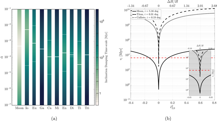
Figure 5. Inclination damping timescale for different satellites of the solar system for oceans of uniform thickness (panel (a)) and with degree 2 thickness variations (panel (b)). Panel (a) shows inclination damping timescales as a function of the ocean's damping coefficient ( ). The value of
  for which the minimum damping timescale is attained and the intervals for which it is below the age of the solar system are indicated with thick and thin marks, respectively. In panel (b) the change in inclination damping timescale as a function of degree 2 ocean thickness variations is shown for the Moon, Titan, and Callisto. In the three cases the
  for which the inclination damping timescale is minimum is used. For the Moon we compute the damping timescale early during its evolution when it had magma ocean and was closer to Earth (a = 20REarth). The dashed red line indicates the age of the solar system.
Download figure:
Standard image High-resolution imageThe case of the Moon is especially interesting. Chen & Nimmo (2016) showed that obliquity tides in a Lunar magma ocean can quickly dampen the Moon's obliquity, making it difficult to reconcile the present Moon's obliquity with the existence of a magma ocean for more than 10 Myr. This contrasts with geochronological constraints that predict life spans up to 200 Myr (see Chen & Nimmo 2016, and references therein). A possible answer to this puzzle can come from ocean thickness variations. Departures from a constant-thickness ocean can increase the inclination damping timescale by several orders of magnitude; for a 50 km thick magma ocean, a thickness difference between pole and equator of just 3 km—of the same magnitude as the Moon's polar flattening—increases the inclination damping timescale from ∼1 to ∼100 Myr (Figure 5(b)). But can we expect the Moon's magma ocean to present such thickness variations?
The Lunar magma ocean solidified in two distinct phases. During the first phase, the magma reached the lunar surface and crystallization occurred from the bottom up. In the second phase, a floating crust formed, slowing down the cooling process. During the first stage, 80% of the magma ocean solidified in about 1000 yr; the remaining 20% solidified during the second stage (Meyer et al. 2010; Elkins-Tanton et al. 2011). Magma ocean variations can arise during both stages. During the first one, rotation can result in latitude-dependent crystallization timescale (Maas & Hansen 2019) and produce bottom thickness variations. Once the crust forms, spatial differences in tidal dissipation within the crust can be expected to produce shell thickness variations.
Similarly, ocean thickness variations can reconcile the present inclination of the outer solar system moons with long-lived oceans. To illustrate this, we consider the cases of Callisto and Titan (Figure 5(b)). The case of Titan is especially interesting, as there is evidence of kilometric shell thickness variations (Lefevre et al. 2014). Equator-to-pole thickness variations of just 1 km,  , are already sufficient to increase Titan's inclination damping timescale from ∼300 Myr to a value higher than the age of the solar system. Similarly, ocean thickness variations of the same order of magnitude can increase the damping timescale of Callisto, providing an alternative explanation to the recent crossing of the 2:1 mean motion orbital resonance with Ganymede proposed in Downey et al. (2020).
3.2.3. The Tidal Response of an Enceladan Ocean
The tidal response of an Enceladan ice shell of variable thickness has been studied using the thin-shell equations (Beuthe 2018, 2019) and using FEM (Souček et al. 2019). In both cases, the effect of ocean dynamics was ignored. Here we will consider the full tidal response (ice shell and ocean) of Enceladus.
We consider the ice-shell and ocean thicknesses to be (Beuthe et al. 2016)


To obtain the tidal response of the ocean and ice shell, we first expand  , χ,
, χ,  , and
, and  in spherical harmonics and afterward solve Equation (29d).
Figure 6 shows the resulting surface displacements. As found in Beuthe (2018) and Souček et al. (2019), ice-shell thickness variations lead to higher-amplitude surface displacements at both the equator and the pole. Moreover, the asymmetry introduced by the degree 3 ice-shell thickness variations translates into a hemispherical asymmetry. The south pole experiences higher-amplitude tides.
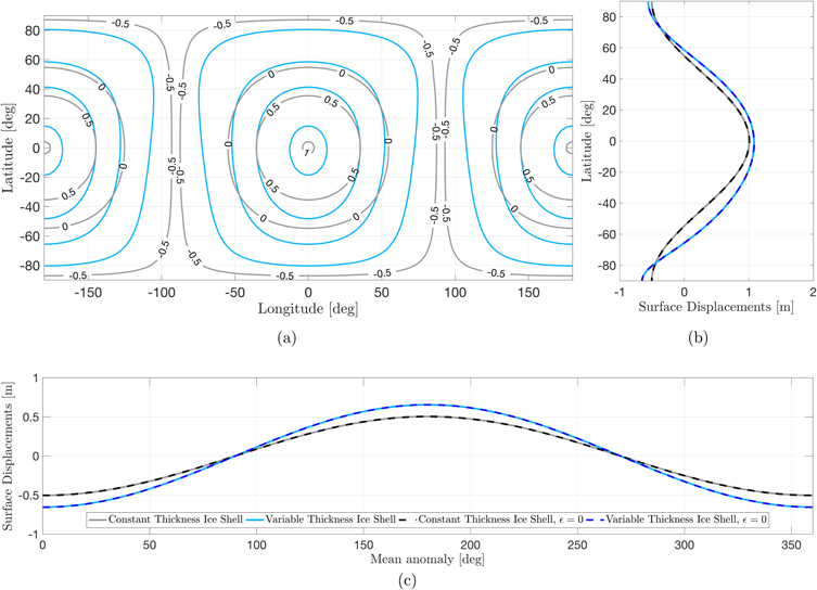
Figure 6. Tidal deformation of Enceladus's ice shell. (a) Surface displacements at t = 0 for an ice shell of uniform (gray) and variable thickness (blue); (b) meridional cut at zero longitude; (c) displacements at the south pole over a tidal period. In all cases, an elastic ice shell is assumed.
Download figure:
Standard image High-resolution imageOur results are very similar to the conductive ice-shell case of Beuthe (2018). This is because the surface displacements obtained considering ocean dynamics and ignoring them ( → 0) are almost identical (Figures 6(b) and (c)), which justifies ignoring ocean dynamics to study the tidal deformation of Enceladus's ice shell if the ocean is unstratified.
3.3. Stratified Ocean of Constant Thickness
We now turn our attention to stratified oceans. As opposed to unstratified oceans, stratified oceans can support internal gravity waves. Internal gravity waves account for around 25% of tidal dissipation on Earth (e.g., Munk & Wunsch 1997). Could they also be of relevance in subsurface oceans?
Tyler (2020, 2011) considered the role of internal waves using the "one-and-a-half layer model," which assumes that a stratified ocean can be modeled by using the equations characteristic of an unstratified ocean provided that an effective ocean depth related to the stratification profile is used (Käse & Tyler 2001). Below we will consider in which cases this approximation can be used.
Our method allows us to compute the tidal response of an ocean with an arbitrary number of layers and an arbitrary density profile. Before proceeding, we need to consider which stratification profile is appropriate for subsurface oceans. Each layer adds two new parameters to the problem (see Table 1). As there are few constraints on the stratification of subsurface oceans, the simpler the model the better. Based on this argument, a two-layer model seems appropriate, but can such a simple model capture the behavior of a subsurface ocean?
It is illustrative to first consider Earth's ocean. The stratification profile of Earth's ocean is normally modeled using a three-layer model that consists of a well-mixed layer at the surface; a thin, strongly stratified thermocline; and the deep ocean, which is weakly stratified (Gerkema 2019). The system can be further simplified if the deep ocean is assumed to be well mixed and the thermocline taken to be very thin. Then, Earth's ocean can be approximated as a two-layer system with a density ratio ρ1/ρ2 ≈ 0.999.
On Earth, solar heating and freezing and melting at the poles drive the global overturning circulation. Together with mixing due to tides, this results in the stratification structure mentioned above. The dynamics of subsurface oceans is very different from Earth's. Yet several mechanisms can lead to ocean stratification. Depending on pressure and salinity, the maximum density of water is not reached at the freezing point but slightly above. This can result in the formation of a cold "stratosphere" beneath the ice shell. Below the cold stratosphere a well-mixed warmer layer can be present. Melosh et al. (2004) estimate that the thickness of the cold stratosphere for Europa's ocean could be a few hundred meters and ρ1/ρ2 ≈ 0.9999. Zeng & Jansen (2021) proposed that the same process can lead to the formation of a stratified layer on top of a well-mixed layer on Enceladus provided that the ocean salinity is low.
On the other end of the spectrum, oceans close to saturation composition can also become stratified. The uptake of salt by buoyant parcels at the seafloor causes upwelling parcels to lose buoyancy before reaching the ice and can produce an ocean divided into a well-mixed warm salty layer below a cold fresh layer of water. Both salinity and temperature gradients decrease upward, and the system can enter the double diffusion convection regime (Vance & Brown 2005; Vance & Goodman 2009).
Finally, a process similar to Earth's overturning circulation might also take place in subsurface oceans. Enceladus ice-shell geometry results in the viscous flow of ice from the equator to high latitudes (Čadek et al. 2019). To maintain the current ice-shell geometry, melting and freezing should occur at the poles and equator, respectively. This can lead to global circulation patterns and a complex lateral and radial stratification profile (Lobo et al. 2021). Lobo et al. (2021) show that these circulation patterns can produce a low-density layer below the ice shell whose thickness changes from 1 to 0 km from pole to equator. The density ratio between the upper and lower layer is ≈0.998. Ashkenazy & Tziperman (2021) showed that the interactions of Europa's ocean with its ice shell can also result in a complex radial and lateral stratification profile characterized by weakly stratified polar regions (r ∼ 0.998) and unstable convective regions in the tropics.
Based on the previous discussion, we will adopt the simple two-layer model. We will first consider the general characteristics of the tidal response of a stratified ocean using the simple two-layer system (Section 3.3.1), and then we will examine the potential contribution of internal tides to Enceladus's heat budget and how it compares with its observed endogenic activity (Section 3.3.2).
3.3.1. Resonances in the Two-layer System
As we did for the one-layer system, we start by considering the nonrotating case. This allows us to find analytical solutions to the equations of motion and study the general characteristics of the ocean response (Appendix E). The eigenfrequencies of the nonrotating system are given by
where r is the density ratio, r ≡ ρ1/ρ2, and to simplify notation we have written  as
as  . Note that
  is simply the ratio between the thickness of layer i and the total ocean thickness (Table 1).
If the ocean is unstratified, r = 1, we recover the eigenfrequencies of the single-layer system—Equation (40). If more layers were added to the system, more internal modes would be added. We can get further insight into the eigenfrequencies of the system by using that, for the moons under consideration, the Lamb parameter is small, → 0. Moreover, we use that the density ratio between the two layers is close to 1, r → 1, but (1 − r)/ is finite. Under these assumptions, Equation (47) reduces to


The first set of eigenmodes ( ) corresponds to the surface gravity waves discussed for unstratified oceans (Section 3.1); the second set (ω2,l
) corresponds to internal gravity waves. As opposed to surface gravity modes, the eigenfrequencies of internal modes are independent of the effective rigidity of the moon and hence the properties of the solid shell. Internal modes are characterized by the difference between the displacements of the density interface and that of the surface, ηd
= η2 − η1. This difference is given by (Appendix E)
) corresponds to the surface gravity waves discussed for unstratified oceans (Section 3.1); the second set (ω2,l
) corresponds to internal gravity waves. As opposed to surface gravity modes, the eigenfrequencies of internal modes are independent of the effective rigidity of the moon and hence the properties of the solid shell. Internal modes are characterized by the difference between the displacements of the density interface and that of the surface, ηd
= η2 − η1. This difference is given by (Appendix E)
If the ocean is unstratified,  , we recover the equilibrium tidal response (Equation (42)). The difference between the surface displacement and that of the interface is proportional to
  . When interface and surface coincide,
  , the difference is zero; in contrast, if the interface is set at the ocean bottom,
  , we recover a zero displacement for it. When the ocean is stratified and close to a resonance,
  and
and  becomes very large. The strength of the resonance depends on the moon's rigidity. We can distinguish between two scenarios. If the moon has a low effective rigidity, Λl
≪ 1, the term proportional to
becomes very large. The strength of the resonance depends on the moon's rigidity. We can distinguish between two scenarios. If the moon has a low effective rigidity, Λl
≪ 1, the term proportional to  is higher than the one proportional to Λl
. The strength of the resonance is then proportional to
is higher than the one proportional to Λl
. The strength of the resonance is then proportional to  the thinner the upper low-density layer is, the weaker the resonance. In contrast, in the rigid-lid limit, Λl
≫ 1, the strength of the resonance is independent of
the thinner the upper low-density layer is, the weaker the resonance. In contrast, in the rigid-lid limit, Λl
≫ 1, the strength of the resonance is independent of  ,
,

In this case, the upper layer remains still and the velocities of the upper and lower layers are opposite in direction,

producing a strong shear. Moreover, the ratio between the magnitude of the velocity of the upper and lower layer is given by the ratio between their thicknesses,  . Plugging Equation (51) into Equation (38), we can obtain tidal dissipation in the two-layer system in the rigid-lid limit
showing that the amount of tidal dissipation in the rigid-lid limit is proportional to the density contrast.
We can recover the one-and-a-half layer system used by Tyler (2011, 2020) if we consider that either layer is much thicker than the other,  or
or  . Equation (48) reduces to

with r
= Ω2
R2/(1 − r)gH1 and r
= Ω2
R2/(1 − r)gH2 for  and
and  , respectively. Comparing Equations (53) and (40), it becomes apparent that the eigenfrequencies of the one-and-a-half layer system are the same as those of the one-layer ocean without a shell and self-gravity with Lamb parameter r
. Furthermore, if there is a rigid lid, Λl
≫ 1, the expression for
, respectively. Comparing Equations (53) and (40), it becomes apparent that the eigenfrequencies of the one-and-a-half layer system are the same as those of the one-layer ocean without a shell and self-gravity with Lamb parameter r
. Furthermore, if there is a rigid lid, Λl
≫ 1, the expression for  (Equation (50)) is the same as what one would obtain in the one-layer system except that
  appears in the denominator instead of
  . Therefore, the two-layer system behaves as the surface-free one-layer system but with = r
if the lower or upper layer is much thicker than the upper layer (
. Therefore, the two-layer system behaves as the surface-free one-layer system but with = r
if the lower or upper layer is much thicker than the upper layer ( or
or  ) and the moon has a high effective rigidity (e.g., Enceladus and Dione). In this case the one-and-a-half layer model of Tyler (2011, 2020) is appropriate to describe the tidal response of a stratified ocean. Solutions of the one-layer system can be used to estimate dissipation in the two-layer system provided that the reduced gravity
  is used instead of the surface gravity to obtain the Lamb parameter and dissipation is scaled with the factor (ρ2 − ρ1)/ρ2.
Resonances with the tidal force occur when  . As we saw for an unstratified ocean of constant thickness, the eigenfrequencies of surface gravity waves are much higher than the diurnal forcing frequency,
  , and hence surface gravity wave resonances do not occur. However, this is not necessarily the case for internal gravity waves. Using Equation (48b), we find the condition for internal gravity wave resonances to be

from which it follows that there exist two different configurations for which a mode of degree l can resonate. From Equation (54) it also follows that resonances of degree l can be excited as far as

The small value of Lamb parameter characteristic of subsurface oceans (Table 2) makes it possible for internal wave resonance to be excited for small density contrasts, r close to 1. In the limit of 1 − r ≫ 4/l(l + 1), Equation (54) reduces to  and
and  . These two resonant thicknesses correspond to the limiting cases of a
  and
and  discussed above in the context of the one-and-a-half layer system. In this limit there exist two resonances, occurring when either the lower layer or the upper layer has r
= l(l + 1).
discussed above in the context of the one-and-a-half layer system. In this limit there exist two resonances, occurring when either the lower layer or the upper layer has r
= l(l + 1).
The previous discussion holds for nonrotating moons. As was the case for unstratified oceans, in nonrotating moons modes of different degrees are not coupled. Therefore, the tidal potential can only excite the degree 2 modes. In contrast, when the Coriolis force is included, a forcing of degree 2 can excite modes of higher degree.
The main characteristics of the tidal response of a two-layer ocean are shown in Figure 7, which shows tidal dissipation in a stratified ocean due to the eccentricity tide for different stratification profiles (r,  ), Lamb parameter (), and rigidity (γ). In all cases, bands of intense tidal dissipation are observed. Each of the bands corresponds to a different resonant mode. As expected from the simple nonrotating case (Equation (54)), given a density contrast, there are two values of
  for which the mode can resonate. We can also observe that when the lower layer is much thicker than the upper layer (
 ), the resonant bands have a slope of ≈−1 in the
  –
– space, as expected from the one-and-a-half layer approximation in the nonrotating case (Equation (53)).

Figure 7. Nondimensional energy dissipation in a two-layer stratified ocean of constant thickness as a function of density contrast (1 − r = 1 − ρ1/ρ2) and layer partition  for different combinations of Lamb parameter and effective rigidity γ (Table 1). Panels (a) and (d) are obtained for values approximately representative of Enceladus and Europa,
  ,
,  , and ξ = 0.
Download figure:
Standard image High-resolution imageThe shape and intensity of these bands depend on the Lamb parameter and the effective rigidity γ. Figures 7(a) and (c) illustrate the effect that the Lamb parameter has on the excitation of internal modes. The Lamb parameter alters the shape of the resonant bands; as decreases, the resonant bands shift to smaller density contrasts. For a given density contrast 1 − r, more resonances can be excited the smaller is. This is expected from the nonrotating model, Equation (55), from which it follows that the lower is, the smaller the density contrast needs to be for a resonance of degree l to be excited.
Figures 7(a) and (b) show how the effective rigidity of the moon also affects the excitation of internal waves. First, we notice that the background tidal dissipation is higher the lower the effective rigidity γ, which follows from the fact that a lower rigidity results in more intense surface gravity waves (see also Figure 2). Second, we observe that the locations of the resonant bands are the same but their intensities decrease, which follows from Equations (48b) and (49). For a hard-shell moon, the strength of the resonances is independent of both effective rigidity and the  for which it occurs. In contrast, for soft-shell moons, the intensity of the resonance depends on
  . As
. As  decreases, the amplitude of the resonance decreases.
We also observe that tidal dissipation depends on the density contrast 1 − r (Equation (52)). This is more evident when the moon has a high effective rigidity and low Lamb parameter (Figure 7(c)). We observe that outside resonances dissipation decreases as 1 − r decreases until it becomes independent of 1 − r when internal waves have a smaller contribution to the energy budget than surface waves. Similarly, the intensity of a given resonance band also decreases with 1 − r.
3.3.2. Tidal Dissipation in a Stratified Enceladan Ocean
In the previous section we considered the tidal response of stratified oceans and showed that internal wave resonances can be excited. We saw that internal wave resonances are stronger for hard-shell moons such as Enceladus and Dione. With this in mind, we will consider the specific case of Enceladus because of its relatively thick ice shell to assess whether internal wave resonances might be behind the moon's thermal activity.
Figure 8 shows tidal dissipation for different stratification profiles and Rayleigh dissipation parameters α and r. For some combinations of ocean stratification and Rayleigh parameter, resonances can result in more tidal heating than Enceladus's thermal output (Howett et al. 2011). For a strongly stratified ocean (1 − r = 10−2), this occurs for α = 10−7 s−1. As the ocean becomes less stratified, dissipation decreases (Equation (52)), and a lower α is required to reconcile tidal heating with Enceladus's thermal output. For a density contrast similar to that used in Lobo et al. (2021) and similar to Earth's, 1 − r = 10−3, an α as small as 10−10 s−1 is required. As α decreases, the dissipation peak becomes sharper, and hence the region of the parameter space for which high values of tidal dissipation are attained narrows. While energy dissipation from internal waves can be close to Enceladus's thermal output, the geographical patterns are characterized by dissipation at low latitudes (Figure 9), which is at odds with the structure of Enceladus's ice shell and the location of the highest endogenic activity at the south pole. Though our model produces a tidal heating distribution that is inconsistent with these observations, it does not preclude the possibility that internal waves are a significant contributor to Enceladus's total thermal budget. The disagreement between predicted and observed heating patterns might indicate that the constant-thickness two-layer model employed is too simplistic. Furthermore, it is uncertain how ocean circulation might redistribute the heat generated as a result of tides.

Figure 8. Tidal dissipation in Enceladus's ocean as a function of Rayleigh coefficient and ocean stratification. The thermal output of Enceladus's south polar terrain is indicated in red (Howett et al. 2011). In all cases, we truncate the system at l = 60.
Download figure:
Standard image High-resolution image
Figure 9. Ocean tidal dissipation patterns for Enceladus for an unstratified ocean due to the eccentricity and obliquity tide (panels (a) and (b)) and two resonant stratified configurations (panels (c) and (d)). In all cases the dissipation pattern is symmetric with respect to the equator and the 0° meridian.
Download figure:
Standard image High-resolution imageIn resonances, strong ocean currents develop. For example, for 1 − r = 10−3,  , and α = 10−9 s−1, velocities of ∼1 m s−1 are attained. When this occurs, nonlinear effects can become important (Hay et al. 2020). This is especially aggravated for internal wave resonances, as a shear develops at the interface between the two layers (Equation (51)), which can lead to Kelvin–Helmholtz instabilities, turbulence, and mixing (Stewart & Dellar 2013). On Earth's oceans the Kelvin–Helmholtz instability plays an important role in ocean mixing and stratification (Smyth & Moum 2012). A similar process might occur in subsurface oceans.
4. Conclusions
In this paper we presented a method to obtain the tidal response of stratified oceans of variable thickness, covered by solid shells that can also vary in thickness. The theory relies on the thin-shell approximations, which allowed us to transform the 3D mass and momentum conservation equations governing the dynamics of the ocean and solid shell to a more tractable set of 2D equations. We solved the resulting equations of motion in the Fourier domain by using a spectral method based on spherical harmonics. This approach allows us to explore the parameter space more efficiently than using numerical techniques such as finite elements, finite differences, or finite volume methods (Hay & Matsuyama 2017, 2019; Rovira-Navarro et al. 2020) and provides more insight into the effect that ocean and shell thickness variations and stratification have on tidal dynamics.
While the thin-shell approximation greatly simplifies the equations of motion, it comes at a cost. Internal inertial waves are filtered out of the system. Rovira-Navarro et al. (2019) and Rekier et al. (2019) showed that the tidal force can excite internal waves in Europa and Enceladus but found that they play a negligible role in the thermal budget of the moons. Nevertheless, nonlinear interactions between internal inertial modes and other ocean flows can lead to instabilities and turbulence (Lemasquerier et al. 2017). We also used the traditional approximation, which has effects on internal wave propagation (see Gerkema et al. 2008; Stewart & Dellar 2010, 2013, for a review).
We first considered the extensively studied case of an unstratified ocean of constant thickness (Tyler 2008, 2009, 2011, 2014, 2020; Matsuyama 2014; Beuthe 2016; Hay & Matsuyama 2017, 2019; Matsuyama et al. 2018). As in previous studies, we showed that the ocean response is given by the combination of surface gravity and Rossby modes. Surface gravity modes can resonate with the tidal force but only for oceans thinner than those expected to exist in the moons of the solar system; in contrast, Rossby waves can be excited by the obliquity tide and lead to significant energy dissipation for moons with high obliquity such as Triton.
We then moved into oceans of variable thickness. As in Rovira-Navarro et al. (2020), we considered the effect that long-wavelength meridional ocean thickness variations have on tidal ocean dynamics. However, the spectral method presented here allowed us to perform a more thorough exploration of the parameter space. We showed that oceans with degree 2 thickness variations respond with the same eigenmodes as oceans of constant thickness. In contrast, oceans with degree 3 thickness variations introduce new modes into the system. But most importantly, we showed that both degree 2 and degree 3 ocean thickness variations hinder the excitation of Rossby waves by the obliquity tide. Rossby waves have been proposed as the leading heating mechanism for Europa (Tyler 2008), Enceladus (Tyler 2009), Triton (Nimmo & Spencer 2015), and early during the Moon's evolution (Chen & Nimmo 2016). Our results show that this is only the case if the oceans do not have deviation from uniform thickness. This is very relevant for the thermal−orbital evolution of moons with subsurface oceans. The decrease in tidal dissipation leads to an increase of the inclination damping timescale, making it possible to reconcile the long-term existence of subsurface oceans with a primordial origin of the inclination for satellites with high inclination such as Titan, Callisto, or the Moon.
We also considered the case of Enceladus, where both ocean and ice-shell thickness variations are expected (Beuthe et al. 2016; Čadek et al. 2016; Hemingway & Mittal 2019), and showed that ocean dynamics have a negligible effect on the deformation of the ice shell. Hence, we can conclude that previous studies that considered the deformation of Enceladus's ice shell while ignoring ocean dynamics provide accurate estimations of tidal deformations of the moon (Beuthe 2018, 2019; Souček et al. 2019).
Finally, we considered the role of ocean stratification. While our method allows us to obtain the tidal response of an ocean with an arbitrary number of layers, we focused on the simplest system: a two-layered ocean. Apart from surface gravity waves and Rossby waves, internal gravity waves can be resonantly excited in a stratified ocean. We find that the strength of the resonances is controlled by the effective rigidity of the satellite, with moons whose shell behaves like a rigid-lid experiencing larger amounts of tidal dissipation due to internal waves. We demonstrate that the one-and-a-half layer approximation used by Tyler (2020, 2011) accurately captures the response of the two-layer system if one of the two layers is much thinner than the other and if the moon has a high effective rigidity.
We then focused on Enceladus and investigated the role of internal waves in the thermal budget of the moon. We found that internal tides can lead to dissipation values of the same order as the moon's observed thermal emissions if the density difference between the two layers is (ρ2 − ρ1)/ρ2 > 10−3. When this occurs, ocean currents of up to 1 m s−1 develop. Very importantly, the currents have different directions in the upper and lower layers, which makes the system prone to the Kelvin–Helmholtz instability (Stewart & Dellar 2013).
Internal waves breaking owing to Kelvin–Helmholtz instabilities play a crucial role in ocean mixing on Earth, which is essential to understand the density profile of Earth's oceans (e.g., Smyth & Moum 2012). Our results underline the connection between tidal dynamics and global circulation in subsurface oceans and the importance of feedbacks between these two elements. For instance, resonant internal waves can lead to enhanced ocean mixing, changing the ocean's density structure, affecting global circulation, and detuning the ocean from the internal wave resonance. Once this occurs, global circulation might restore the resonant stratification profile and bring the ocean back to a resonant configuration. We can speculate that this might cause alternation of periods of high- and low-amplitude internal tides.
The method presented here opens the door to tackle new problems. Based on existing data on shell thickness variations for Enceladus, we focused on meridional thickness variations. Sectoral and tesseral thickness variations might also occur; we can expect these variations to introduce new modes into the system—in a similar way to degree 3 meridional thickness variations. Most notably, we have left the interaction between baroclinic and barotropic tides in oceans with bottom and shell topography out of this study. On Earth this process accounts for ∼30% of energy dissipation via the excitation of internal waves, and thus we have reasons to suspect that it can also be of importance in other ocean worlds.
M.R. and I.M. were supported by the National Aeronautics and Space Administration (NASA) under grant No. 80NSSC20K0570 issued through the NASA Solar System Workings program. H.H. was supported by the National Aeronautics and Space Administration (NASA) through the Europa Clipper project. A portion of the research was carried out at the Jet Propulsion Laboratory, California Institute of Technology, under contract with NASA. The authors thank two anonymous reviewers for their helpful comments on the manuscript.
Appendix A: Laplace Tidal Equations

Appendix B: Spherically Symmetric Solid Shell
Equations (29d) are significantly simplified if we consider a solid shell with uniform properties ( for l ≠ 0 and m ≠ 0). In such cases, we can use Equations (29c) and (29d) to eliminate
  and
and  from the equations. The pressure load exerted by the shell
  is then given by
where Λl is a nondimensional spring constant (Beuthe 2016, 2018)


 follows from the extensional rigidity of the shell, and
  accounts for bending effects. Plugging Equation (B1) into Equations (29a) and (29b), we get
Appendix C: Approximated Solution for Westward Obliquity Tides
In case the ocean has only degree 2 thickness variations, we can still find an approximation for the westward obliquity tide by cutting the solution at degree 2:
The previous expression reduces to Equation (43) if  .
.
Appendix D: Love Numbers of a Uniform Solid Body
The gravitational and radial displacement Love numbers of a homogeneous body are given by (Matsuyama et al. 2018)
with

As shown in Beuthe (2016), the pressure Love numbers are a linear combination of the tidal and load Love numbers

Using the previous expressions, we compute υT, υL, and υP for different values of  (Figure 10). The value of υ is smaller than 10−1 for all the moons considered, even if we assume a very deformable core for the smallest moons.
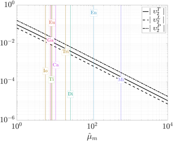
Figure 10. Effect of a nonrigid mantle in the tidal response of the ocean and shell.  is computed assuming a Young modulus for the core of E = 170 GPa for all moons except for the mid-sized Saturnian moons, for which we assume a soft deformable core, E = 17 GPa. The core is considered to be homogeneous, and its density is calculated self-consistently to satisfy the mean density constrain.
Download figure:
Standard image High-resolution imageAppendix E: Solution for the Nonrotating Two-layer System
In this appendix, we obtain the surface displacements for the two-layer system in the rigid-lid approximation for a nonrotating ocean. The dynamics of the two-layer system is given by (Equation (8))


We introduce  and assume a solid shell of constant thickness. By taking ∇ · of Equations (E1c) and (E1d) and using the continuity equations (Equations (E1a) and (E1b)), we can obtain two equations for
  and
and  :
:
From Equation (E2a) we can obtain  :
:
We can simplify the previous equation by considering that the ocean is far from surface wave resonances,  , and noting that (1 − r ≪ 1). Doing so, we find
where we have neglected terms of order 2, (1 − r)2, and (1 − r). Unless there is an internal wave resonance, the first term is much higher than the others; the upper layer approximately follows the equilibrium tide. Plugging Equation (E4) into Equation (E2b), we can obtain an expression for  :
:
Appendix F: Differential Operators
The following differential operators appear in the main text:


with  . If a and b are expanded in spherical harmonics, the differential operators can be rewritten as

where  ,
,  , and
, and  are defined in Appendix G.
To ease notation in the equations, we define the coefficients:
Appendix G: Spherical Harmonic Tools
Apart from scalar spherical harmonics, we will need to use vector spherical harmonics and their properties (e.g., James & Cook 1976; Ivers & Phillips 2008). The vector spherical harmonics  are given by
the matrix represents a Wigner 3-j coefficient. Vectors e μ are defined in terms of the unit vectors of Cartesian coordinates (1x ,1y ,1z ) as
In spherical coordinates, the vector spherical harmonics can be written as


Using the previous equations, we can write the gradient and curl of a spherical harmonic as
To ease notation, we will also use


To project the equations onto spherical harmonic basis, the following relations are needed: First, we define the projection of two fields G and F as

where G * is the complex conjugate of G . The scalar and vector spherical harmonics are orthogonal and satisfy the properties


with δ being the Kronecker delta function.
We can use the properties of scalar and vector spherical harmonics to project Equation (A1) onto spherical harmonic basis. If we have two scalars,


the following properties hold:


with (James & Cook 1976)
The 2 × 3 arrays between parentheses and curly brackets are Wigner 3-j and 6-j symbols, respectively, and Λ is given by

For the special case (lν , mν ) = 0, we have


From the properties of 3-j symbols, the only nonzero coupling coefficients are those satisfying ∣mα ∣ ≤ lα , ∣mβ ∣ ≤ lβ , ∣mν ∣ ≤ lν , mν = mβ + mα , and ∣lα − lν ∣ ≤ lβ ≤ ∣lα + lν ∣, from which it follows that the Coriolis term and zonal property variations couple terms of equal order but different degree. In contrast, if there are sectoral or tesseral ocean thickness variations, equations of different order are also coupled.
Appendix H: Benchmark against FEM Solution
Rovira-Navarro et al. (2020) obtained the solution to the LTEs for oceans of variable thickness using FEM. We use the solutions obtained in Rovira-Navarro et al. (2020) for an Enceladan ocean of variable thickness to benchmark the semianalytical method. As seen in Figure 11, the solution obtained using FEM and that using the semianalytical approach are equivalent.
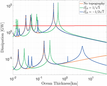
Figure 11. Tidal dissipation in an Enceladan ocean of variable thickness obtained with the method presented in this article (solid lines; Section 2.2) and the FEM method used in Rovira-Navarro et al. (2020; filled circles). The comparison is done by turning off self-gravity.
Download figure:
Standard image High-resolution image