Progenitors of Low-redshift Gamma-Ray Bursts

Vahé Petrosian; Maria G. Dainotti

doi:10.3847/2041-8213/ad2763

1. Introduction

Since the discovery of gamma-ray bursts (GRBs) by Vela satellites several instruments on board multiple satellites (Compton Gamma Ray Observatory (CGRO), Beppo-Sax, Fermi, Swift, Konus-Wind, and others) have detected more than a thousand GRBs, the majority of which are classified as long GRBs (LGRBs) and most of the rest as short GRBs (SGRBs). A good fraction of these GRBs have measured spectroscopic or photometric redshifts, or redshifts based on host galaxies. The bimodal distribution of the observed duration, T₉₀, of GRBs was established first by Konus-Wind (Mazets et al. 1981) and later by the BATSE instruments (Kouveliotou et al. 1993) of CGRO, dividing them into two classes of SGRBs and LGRBs separated at T₉₀ = 2 s. However, the value of dividing T₉₀ is somewhat uncertain. A different classification of GRBs observed by Swift in Bromberg et al. (2013), obtains a dividing of T₉₀ ∼ 0.8 s. There are other features separating the two classes. LGRBs on average have softer spectra than SGRBs, as measured either by their spectral hardness ratio (HR) or the value of E_p, the photon energy at the peak of the ν f(ν) energy spectrum.⁸ Localized LGRBs are often associated with star-forming galaxies and regions, while SGRBs are typically found in older systems and away from star-forming regions (see the review by Berger 2014). These dichotomies have led to two distinct progenitors. LGRBs are believed to be produced by supernova (SN) explosions of massive Wolf–Rayet stars (see the review of Langer et al. 2010 and the famous case of GRB 021004, Mirabal et al. 2003; and GRB 060218, Campana et al. 2006; Waxman et al. 2007), so that their formation rate (FR) is expected to follow the cosmic star formation rate (SFR). SGRBs, on the other hand, are believed to have been produced during neutron star (NS)–NS or NS–black hole (BH) mergers; thus their FR is expected to follow a delayed form of the SFR. Such mergers are also expected to lead to kilonovae and produce gravitational waves (GWs). Recent association of a GW source with SGRB 170817A (Abbott et al. 2017; Goldstein et al. 2017; Pian et al. 2017; Savchenko et al. 2017; Troja et al. 2017) has firmed this belief. The left panel of Figure 1 shows a recent determination of the cosmic SFR by Madau & Dickinson (2014) and examples of the delayed SFR from Paul (2018), assuming a power-law distribution of the delay time, ${\rm{\Phi }}{({\tau }_{d})\propto ({\tau }_{d}/{\tau }_{0})}^{-n}$ , with power-law index n.

**Figure 1.** Left: cosmic SFR from most comprehensive compilation by Madau & Dickinson (2014) and two examples of delayed SFR with power-law distribution of delay times, ${\rm{\Phi }}{({\tau }_{d})\propto ({\tau }_{d}/{\tau }_{0})}^{-n}$ , with indexes n = 1.0 and 3.0; from Paul (2018). Right: results of five independent determinations of LGRB FR of somewhat different samples, in the redshift range ∼1.5 < z < 4, using the EP-L method, all normalized at the peak value of the observed SFR (black solid line with selected error bars): from the top, (a) magenta, Lloyd-Ronning et al. (2019); (b) cyan, Yu et al. (2015); (c) green, Tsvetkova et al. (2017); (d) red, Petrosian et al. (2015); and (e) blue, Pescalli et al. (2016). With different degrees, all are showing higher LGRB FR than the SFR at low redshift (see the text for more detailed comparison of these works).
Download figure:
Standard image High-resolution image

**Figure 1.** Left: cosmic SFR from most comprehensive compilation by Madau & Dickinson (2014) and two examples of delayed SFR with power-law distribution of delay times, ${\rm{\Phi }}{({\tau }_{d})\propto ({\tau }_{d}/{\tau }_{0})}^{-n}$ , with indexes n = 1.0 and 3.0; from Paul (2018). Right: results of five independent determinations of LGRB FR of somewhat different samples, in the redshift range ∼1.5 < z < 4, using the EP-L method, all normalized at the peak value of the observed SFR (black solid line with selected error bars): from the top, (a) magenta, Lloyd-Ronning et al. (2019); (b) cyan, Yu et al. (2015); (c) green, Tsvetkova et al. (2017); (d) red, Petrosian et al. (2015); and (e) blue, Pescalli et al. (2016). With different degrees, all are showing higher LGRB FR than the SFR at low redshift (see the text for more detailed comparison of these works).
Download figure:
Standard image High-resolution image

These dichotomies can be further tested by comparing the distributions of their intrinsic characteristics, mainly the luminosity function (LF), and luminosity and FR evolutions, L(Z) = L₀ g(Z) and $\dot{\rho }(Z)$ , where g(Z) describes the luminosity evolution and L₀ is the normalization. All these features can be described by the bivariate distribution Ψ(L, Z).⁹ In particular, a clearer picture of FRs of GRBs can provide a better estimation of rate of occurrence of low-mass merger GW sources and kilonovae, especially at low redshifts, that are within the reach of current detectors.

The main goal of this Letter is to determine the FR of GRBs, $\dot{\rho }(Z)$ , at low redshifts, Z < 3. In the next section, we describe the method we use to this end, and in Section 3 we review results obtained for FR of GRBs using this method and present evidence indicating that low-redshift LGRBs could also have compact star mergers as progenitors, which would increase the expected rate of GW sources and kilonovae. A brief summary and conclusions are presented in Section 4.

2. The Basic Problem and Procedures

To achieve the abovementioned goal, we need an accurate description of the bivariate LF, Ψ(L, Z). This, of course, requires samples of GRBs with known redshifts,¹⁰ and a knowledge of all observational selection effects, which truncate the data and introduce bias. The attempts to correct for this bias, known as the Eddington or Malmquist bias, has had a long history. Early attempts, and a majority of current ones dealing with GRBs, have used parametric forward fitting methods, whereby a set of functional forms are fit to the data to determine the "best-fit values" of the parameters, using χ² or maximum likelihood algorithms. These methods assume parametric forms for several functions: the spectrum, light curves, g(Z), and $\dot{\rho }(Z)$ , each with three or more parameters, raising serious questions about the "uniqueness" of the results. Also, they often require binning and thus large samples, which is not always the case, especially for SGRBs. There are several "non-parametric, non-binning methods" (e.g., the $V/{V}_{\max }$ , Schmidt 1968; C⁻, Lynden-Bell 1971) that are more appropriate for small samples. However, a major drawback of these methods is the "ad hoc" assumption of "independent or uncorrelated variables," which for extragalactic sources means no luminosity evolution, i.e., g(Z) = const. For more details, see a review by Petrosian (1992). To overcome this shortcoming, Efron & Petrosian (1992, 1998) developed new methods (hereafter called the EP method), whereby one first determines whether L and Z are correlated or not. If correlated, then it introduces a new variable L₀ ≡ L/g(Z) and finds the luminosity evolution function, g(Z), that yields an uncorrelated L₀ and Z, whose distributions, LF ψ(L₀) and FR $\dot{\rho }(Z)$ , can be obtained using, e.g., the Lynden-Bell C⁻ method. The advantage of this combined EP-L method is that the two evolutions are obtained directly from the data, non-parametrically and without binning.¹¹ In the past, these methods have proven to be very useful for studies of GRBs (Lloyd & Petrosian 1999; Lloyd-Ronning & Ramirez-Ruiz 2002; Yonetoku et al. 2004; Kocevski & Liang 2006; Dainotti et al. 2013, 2015, 2017a, 2017b, 2020, 2021a, 2021c, 2022c), and active galactic nuclei; see, e.g., Dainotti et al. (2022a), Singal et al. (2022).

3. Results on Formation Rates

In this section, we present results from more recent works on the FR of GRBs using the non-parametric EP-L method. As emphasized earlier, this method requires a sample with a measured redshift and well-defined observational selection effects; such samples are referred to as "complete." Most instruments have a relatively well-defined gamma-ray peak flux threshold. With careful selection, one can obtain a somewhat complete sample. However, securing a redshift is a complicated process and includes several other observational selection effects that are not as easily quantified as the peak flux limit. Swift has been most successful in attempting to quantify these effects. After the Burst Alert Telescope trigger, the X-ray Telescope, on board Swift, provides a more accurate localization. This is especially true for sources with higher X-ray fluxes. This introduces addition selection effects based on the X-ray flux limit. Then, the optical-UV telescope attempts to provide a more accurate position. The higher-resolution localization is transmitted to ground-based telescopes for the identification of a host galaxy and further redshift measurement.

This third step introduces greater complexity. Quantifying the selection bias and conducting population studies becomes challenging due to the difficulty of obtaining observing time at large-aperture telescopes for a large number of GRBs.

3.1. The Samples

The samples of GRBs with known redshift used in the following two subsections for our analysis are taken from Petrosian et al. (2015) for the LGRBs, and from Dainotti et al. (2021d) for the SGRBs. The relative numbers of different classes are shown in Figure 2. In addition to LGRB (purple) and SGRB (blue) samples, we include a subclass of LGRBs, called intrinsically short, that are classified as SGRBs based on their rest-frame duration, ${T}_{90}^{\mathrm{rest}}={T}_{90}^{\mathrm{obs}}/Z\lt 2\,{\rm{s}}$ (denoted as IS, yellow).¹² The red part shows the fraction of all LGRBs observed to be associated with Type Ib/c SNe. Of the hundreds of GRBs annually observed, the fraction linked with SNe spectroscopically or photometrically vary from ${f}_{\mathrm{SN}}\sim 2 \% \mbox{--}7 \%$ (Dainotti et al. 2022b; Rossi et al. 2022). For example, in the sample used by Petrosian et al. (2015) for the investigation of the low-z excess described below, 16 of 207 LGRBs are associated with SNe, giving ${f}_{\mathrm{SN}}=7.7 \%$ . However, there is a strong bias in detection of SNe at high redshift and most of these associations are with low-redshift LGRBs. Thus, the abovementioned fraction must be a lower limit. Addressing this problem accurately requires an investigation of the joint distribution of luminosity and redshift of GRBs and SNe, which in turn demands a sample of sources with well-defined criteria for selecting both types of sources. In general, the quality of data on SNe associated with GRBs is highly variable, and there are no such samples. As a result, we can rely on rough estimations of the fraction at low redshifts, specifically z < 0.5, where the abovementioned bias is less severe. We will return to this issue after describing our results.

**Figure 2.** The pie chart showing the LGRBs in purple, SGRBs in blue (with intrinsically short (IS) in yellow) adopted from Petrosian et al. (2015) and Dainotti et al. (2021d), respectively. The red shows fraction of all LGRBs for which the associated Type Ib/c supernovae have been observed.
Download figure:
Standard image High-resolution image

3.2. LGRBs

The right panel of Figure 1 shows five results from five independent analyses. Four of these analyses use different samples of Swift LGRB data and one (in green) employs Konus-WIND LGRB data (Tsvetkova et al. 2017). It should be emphasized that none of the samples used in these works are strictly speaking complete, because of the difficulty in quantifying the completeness in redshift with the currently available samples.¹³ Yu et al. (2015) analyze a sample consisting of 127 Swift LGRBs with well-measured spectral parameters from Fermi Gamma-ray Burst Monitor (GBM) and Konus-Wind, and use the Swift nominal γ-ray peak flux threshold. Tsvetkova et al. (2017) used a sample composed by 150 Konus-Wind LGRBs. The sample from Lloyd-Ronning et al. (2019) is composed of 376 LGRBs with known redshifts.¹⁴ Instead of peak flux and luminosity, they used fluence and isotropic energy, _iso, along with several observed correlations. Petrosian et al. (2015) obtained FRs using only the gamma-ray threshold, and using both gamma-ray and X-ray thresholds (based on X-ray flux compilation by Nysewander et al. 2009). The latter, which, yields a significantly different FR history than the former, especially at midrange redshifts, is presented here. In addition, to account for more unknown optical selection bias, Petrosian et al. (2015) used a gamma-ray threshold 10 times larger than the nominal Swift threshold. The sample studied in Pescalli et al. (2016) is composed of several subsamples: a sample of 52 LGRBs of low luminosity complete in redshift taken from Salvaterra et al. (2012); an intermediate luminosity sample composed of six GRBs, and a high-luminosity sample taken from Wanderman & Piran (2010), which collects GRBs detected by Swift from its launch until GRB 090726, all with a measured peak flux and a measured redshift. Their total sample has 80% redshift completion. As evident, all of these estimates of FR of LGRBs deviate significantly, though with different degrees, from the cosmic SFR at Z < Z_c ∼ 3 or z < ∼ 2.

However, it should be noted that Pescalli et al. (2016) claim no significant deviation because they find only a 1.5σ deviation from an earlier determination of the cosmic SFR, which is flatter (at low redshifts) than the more recent determination of SFR by Madau & Dickinson (2014) shown in Figure 1. This clearly raises the significance of this deviation. For example, at $\mathrm{log}Z=0.13$ Pescalli et al. (2016) give a value $\mathrm{log}\dot{\rho }\,=-{0.27}_{-0.14}^{+0.09}$ and Madau & Dickinson (2014) give $\mathrm{log}\dot{\rho }\,=-0.62\pm 0.07$ . Adding the two errors in quadrature, we obtain $\sigma =\sqrt{{0.14}^{2}+{0.07}^{2}}=0.15$ , indicating 0.35/0.15 ∼ 2.3σ deviation. This the smallest detected deviation of the five papers. The largest deviation, >10σ at z ∼ 0.5, is obtained by Lloyd-Ronning et al. (2019).

It should also be noted that all five papers find a 2σ to 3σ correlation between luminosity and redshift, indicating presence of luminosity evolution with g(Z) = Z^α (2 < α < 3). The FR evolution presented above corrects for this correlation. Petrosian et al. (2015), in their Figure 4, show the FR ignoring the luminosity evolution. As expected they find an increase in the FR at large redshifts, but the excess at low redshift relative to the SFR remains significant.

In the left panel of Figure 3, we compare the average value of the logarithms of the above five FR estimates with the cosmic SFR. This average, not significantly different from the estimate by Petrosian et al. (2015), which includes both gamma-ray and X-ray observational biases, clearly deviates from the SFR by 9σ at the lowest redshift (z = 0.15) and 5σ at z ∼ 1. Thus, we are led to suggest the presence of two LGRB components at redshifts below Z_c: the first component (component 1) follows the cosmic SFR, while the second component (component 2) at low redshift, shown by the solid and dashed blue curves, is obtained from subtracting the first component from the observed average and Petrosian et al. (2015) FR redshift distribution, respectively. Both, again, are normalized at the peak of the cosmic SFR.¹⁵ The important question is what are the progenitors of these two components. The progenitors of component 1 are most likely collapsars. Assuming that the flat portion of the average FR below Z_c ∼ 3 is at ${\dot{\rho }}_{0}=1$ , the total rate integrated over 0 < Z < Z_c will be equal to Z_c − 1. For component 1, with $\dot{\rho }{(Z)\simeq {\dot{\rho }}_{0}(Z/{Z}_{c})}^{2.7}$ , the total FR will be Z_c/(2.7 + 1) = 0.27Z_c, yielding a fraction 0.27Z_c/(Z_c − 1) ∼ 40% ± 5% (uncertainty based on SFR data). (This is the average fraction but the actual fraction varies from 100% at Z_c to 50% at Z = 1.5, where the black and magenta curves intersect, to a minimum of 13% at the lower bound of Z = 1.15.) Thus, all such associations are included in component 1 and subtracted from the total.

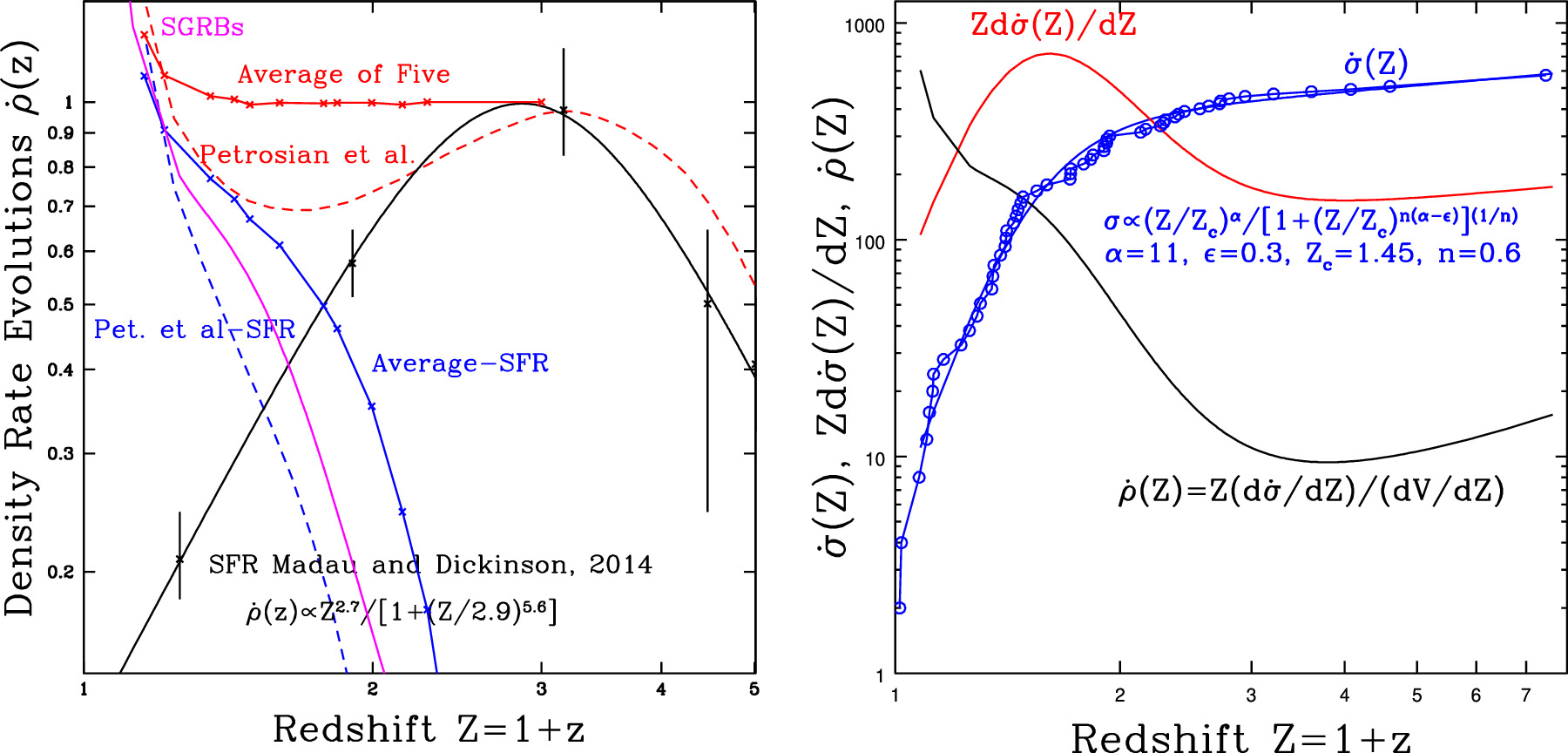
**Figure 3.** Left: same as Figure 1 left but showing the average value of five independent estimates plus Petrosian et al. (2015) results in red. The blue lines show the two low-redshift components obtained by subtracting the cosmic SFR from the observed ones. The magenta is the FR of SGRBs described in the right panel. Right: FR of SGRBs using most recent Swift sample of SGRBs with known redshift, using the procedures described in Dainotti et al. (2021c). Here σ(Z) is the cumulative (>Z) redshift distribution corrected for observational selection effects (blue dots), with arbitrary normalization. The blue curve is a smoothly broken power-law fit (with indicated form and parameters of the fit), from which we obtain the FR, $\dot{\rho }(Z)$ analytically as described in the text.
Download figure:
Standard image High-resolution image

The remaining question then is what are the progenitors of LGRBs in component 2, which includes ∼60% ± 5% of 1.15 < Z < Z_c LGRBs. As evident, the FR of this component decreases rapidly with increasing redshift, in a manner similar to the delayed SFR rates, shown in the left panel of Figure 1, expected for compact mergers. In addition, this component has a shape almost identical to that of SGRB FR, shown by the magenta curve in the left panel of Figure 3 (described in the next section), providing further support for the merger progenitor scenario, which can also result in GW sources and kilonovae. There are no confirmed association of LGRBs with GW sources, but as described below two low-redshift LGRBs have associated kilonovae, indicating that some fraction of component 2 sources have compact merger progenitors. To shed some light on this fraction, we now revisit the fraction of LGRBs associated with SNe. As mentioned above there are many uncertainties on this issue, and small fraction of all 1.15 < Z < Z_c LGRBs have association with SNe confirmed spectroscopically. However, since finding associated SNe is difficult at high redshifts, most such associations are in low redshifts. We address this problem limiting our investigation to the Z > 1.15 region because the abovementioned estimates of LGRB FRs do not provide any information below this redshift. To minimize the redshift bias, we consider two low-redshift ranges using two data sets. One is an earlier compilation by Hjorth & Bloom (2012) that includes 26 LGRBs, with measured redshifts (25 if we do not consider the shockbreaout GRB 060218), where the associations are graded from A to E, with A being spectroscopically verified and decreasing to highly uncertain at C, D, and E grades. In the redshift range 1.15 < Z < 1.5 there are five sources with only one grade A giving ${f}_{\mathrm{SN}}\sim 20 \%$ . But if we include the two grade Bs, i.e., not spectroscopic verified sources, the fraction rises to ${f}_{\mathrm{SN}}=60 \%$ . These are small number subject to large statistical uncertainties so that this fraction could be in the range ∼20%–100%.¹⁶ In the wider range of 1.15 < Z < 2.0, there are 19 sources with six having grades A and B, yielding a lower fraction ${f}_{\mathrm{SN}}=32 \%$ . In a recent work consisting of larger number (71) LGRB-SN sources, Dainotti et al. (2022b) classified them as A, AB, B, etc. Of 15 sources in the 1.15 < Z < 1.5 range there are three A sources, resulting in a fraction of 20%. But adding two AB sources raises the fraction to 32%. In the wider range, 1.15 < Z < 2.0, consisting of 43 sources there are no more A sources but two more ABs, yielding ${f}_{\mathrm{SN}}=7/43=16 \%$ . Given statistical errors of few %, both these fractions are consistent with the 30% we obtained above using the numbers in our Figure 2. Thus, the remaining 70% in this range or 60% ± 5% in the whole range, 1.15 < Z < 3, could have non-collapsar, most likely compact mergers, progenitors.¹⁷

3.3. SGRBs

The discoveries of GW sources and the associations of with SGRBs and kilonovae, mentioned above, have made the determination of the FR of SGRBs a critical issue, and has led to an increased activity on this front (e.g., Wanderman & Piran 2015; Ghirlanda et al. 2016; Abbott et al. 2017; Paul 2018; Zhang & Wang 2018). These are all based on the parametric forward fitting method described above. More recently, Dainotti et al. (2021c) have used the non-parametric EP-L method, for determining the FR of SGRBs, which we now described briefly. There are in general smaller numbers of SGRBs than LGRBs and even smaller samples with known redshifts. The sample size is important. For a larger sample one can obtain more reliable and detailed results, no matter what method is used. However, as emphasized above, the observational selection that affects one's ability to determine the redshift is even more critical. The most important selection criteria is having a complete sample with a well-defined gamma-ray peak flux threshold. In the absence of X-ray observations and due to small numbers, the more complete and conservative method used by Petrosian et al. (2015) cannot be used for SGRBs. As an efficient alternative to overcome the paucity of the sample, Dainotti et al. (2021c) use a statistical method (the well-known Kolmogorov–Smirnov (KS) test) to find the lowest-possible flux threshold, hence securing the largest sample. This ensures that the subsample with redshift was drawn from the complete parent sample including all SGRBs (with and without redshifts). We have repeated this procedure with a slightly larger SGRB sample. The results from this work are presented in the right panel of Figure 3. In general, the EP-L method yields cumulative distributions of the variables, in this case the rate, $\dot{\sigma }(Z)$ , of sources with redshift >Z, related to the differential rate as

$\begin{eqnarray}&&\dot{\sigma }(Z)={\int }_{1}^{Z}Z{{\prime} }^{-1}\dot{\rho }(Z^{\prime} ){dV}/{dZ}^{\prime} ,\end{eqnarray} \tag{ 1 }$

where V(Z) is the comoving volume up to redshift Z.

The results are shown by the blue points and are fit by a broken power law, the parameters of which are given in the figure. The black line shows the redshift evolution of the FR obtained from differentiating Equation (1) and the analytic form for $\dot{\sigma }(Z)$ . This FR is shown by the magenta curve in the left panel, normalized to the others at the lowest redshift. As is evident, it has a form very similar to that of the FR of the low-redshift component of LGRBs.

This further supports the above hypothesis that both SGRBs and approximately 60% of low-redshift, Z < Z_c, LGRBs have a common progenitor. The fact that these FRs are similar to delayed SFRs lead us to conclude that mergers of compact stars (NSs and BHs) are the progenitor of almost all low-redshift GRBs, except for ∼40% of Z < Z_c LGRBs, of which some are associated with SNe). This hypothesis has received strong support from new observations showing coincidence in time and space of kilonovae with two low-redshift LGRBs. The first is GRB 211211A, with z = 0.076 and T₉₀ > 30 s, observed by Rastinejad et al. (2022). In addition, Fermi Large Area Telescope observations of this source show a transient gamma-ray emission (duration 20 ks) starting about 1 ks after the trigger that is interpreted to be due to inverse Compton scattering of the kilonova optical/near-infrared photons by the GRB jet accelerated electrons (Mei et al. 2022). The second is the extremely bright GRB230307A observed by JWST (Levan et al. 2023a, 2023b) and discussed by Wang et al. (2023), with z = 0.0646 and T₉₀ ∼ 35 s (observed by Fermi-GBM and several other instruments), that could be produced by a compact star merger, and as claimed by Wang et al. (2023) is associated with a kilonova very similar to that of GW merger GW170817 (Abbott et al. 2017). These pieces of evidence complement the results presented here based on population studies.

4. Summary and Conclusions

In this Letter we have explored how the FRs of LGRBs and SGRBs compare with cosmic SFR. The general expectation is that LGRBs produced by collapsars (SN explosions of massive Wolf–Rayet stars) should follow the SFR, while the FR of SGRBs, produced by merger of compact stars (NSs and BHs), should be delayed relative to SFR (Figure 1, left).

1.
We describe methods used for obtaining the FR history of extragalactic sources and the advantages of the non-parametric, non-binning Efron–Petrosian–Lynden-Bell method. This approach obtains the cosmological distributions and evolution of sources, yielding the rate of luminosity evolution, the luminosity function, and the FR evolution, especially for small sample of sources with complex observational selection biases.
2.
We present results on five independent determination of the FRs of different samples of LGRBs. Each analysis uses the EP-L method, showing significant deviations, from SFR at low redshifts, albeit to different extents, (Figure 1, right).
3.
Taking the logarithmic average of the five determinations of the LGRB FR, we divide it into two components; component 1 that follows the cosmic SFR (consisting of ∼40% ± 5% of Z < Z_c ∼ 3 LGRBs) and the rest as component 2 whose FR decreases rapidly with increasing redshift, in a manner expected from delayed SFR (Figure 3, left).
4.
Furthermore, we present a new determination of FR of SGRBs, again using the EP-L method, and the data selection procedure described in Dainotti et al. (2021c) and in the right panel of Figure 3. This FR is almost identical to that of the low-redshift component 2 of LGRBs (Figure 3, left).

There are some caveats that should be noted.

1.
First, we have shown similarities between the shapes of FRs, but further study is required to determine the fraction of LGRBs and SGRBs that can be attributed to merger events.
2.
Second, some low-z LGRBs are associated with SNe and thus, most likely, are not merger events. However, as described in connection with the pie chart of Figure 2, the fraction of LGRBs with such associations is <10%. We also point out that many LGRB-SN associations reported in the literature are uncertain, because they are based only on observed bumps in their light curves rather than spectroscopy. We use two compilations where the authors classify such associations by varying degrees (grades) of confidence. Using these classifications in a more recent and larger sample the range 1.15 < Z < 1.5 (to minimize the redshift bias), we find fractions ${f}_{\mathrm{SN}}\sim 30 \%$ , consistent with our result that shows that 30% of the first component is within this range. It should be noted that given the large uncertainty there is some small probability that all or most of component two LGRBs are associated with SNe and not due to mergers. This, however, raises the even more puzzling issue of why they do not follow the SFR. The merger scenario seems a simpler possibility.
3.
Third, Bromberg et al. (2013), using a sample composed of BATSE data from 1991 April until 2000 August, Swift data from 2004 December until 2012 February, and Fermi data from 2008 until 2010 July, claim that a fraction of SGRBs could have a collapsars as progenitors. However, as shown in their Figure 4, the numbers there are very small. In addition, this claim is somewhat uncertain and depends strongly on the spectral hardness of the GRBs. It requires determination of the bivariate distribution of duration T₉₀ and hardness ratio HR, denoted as Φ(T₉₀, HR). Investigating this joint distribution is far beyond the scope of our paper.
4.
Finally, LGRBs are often found in low-metallicity galaxies, which could have different FR than the cosmic SFR. To first order one would expect a higher FR for LGRBs at high redshifts, with more metal-poor galaxies, rather than low redshifts, the main focus of our paper.

In summary, we have presented evidence for significant, and almost identical, deviations of the FRs of both LGRBs and SGRBs from SFR at low redshifts. These deviations have the form expected from the delayed SFR. The latter similarity is qualitative only, because the assumption of power-law distributions of delayed time used in Paul (2018) is questionable. For example, Wanderman & Piran (2015), in addition to power-law distributions, test lognormal distributions. There are other possibilities not explored yet.

Our main conclusion is that a relatively large fraction of the low-redshift LGRBs, like the SGRBs, most likely have compact merger progenitors. An independent observation supporting this scenario, based on population study, emerges from two recent discoveries of association of low-redshift LGRBs with kilonovae.

For the future, it will be useful to conduct a more quantitative comparison of the FR of low-redshift GRBs with different delayed scenarios. This will aid in determining the most accurate delay mechanism. Discovery of more association of low-redshift LGRBs and kilonovae will also provide valuable insights.

Progenitors of Low-redshift Gamma-Ray Bursts

Article metrics

Author affiliations

ORCID iDs

Dates

Abstract

1. Introduction

2. The Basic Problem and Procedures