


Abstract
The network structure seen in the solar images is the outline of supergranulation, which is the large-scale convection in the Sun with a size of about 30 Mm and a lifetime of 24 hr. We have obtained the supergranulation lane widths from the autocorrelation function of image windows from the Ca ii K spectroheliograms. The images are obtained from the 100 yr Kodaikanal data, which contains information on more than nine solar cycles. The lane widths are known to show a positive correlation with the sunspot number. It is now found that the lane widths, obtained near the mid-latitudes during the sunspot cycle minima, are strongly correlated to the following sunspot number maxima. A straight-line fit adequately describes the variation. It is also found that the correlation is weak or insignificant at other times. The strong correlation of the two parameters thus provides a simple way to predict the maximum sunspot number about 4–5 yr in advance. The results are important in space weather predictions and solar irradiance variations.
Export citation and abstract BibTeX RIS

Original content from this work may be used under the terms of the Creative Commons Attribution 4.0 licence. Any further distribution of this work must maintain attribution to the author(s) and the title of the work, journal citation and DOI.
1. Introduction
A network-like structure in the chromospheric lines has been known since the 1890s and remained enigmatic for a long time. Hart (1954) found a cellular pattern in the velocity distribution over the solar disk. Pioneering studies by Leighton et al. (1962) and Simon & Leighton (1964) have shown that the network arises due to magnetic flux concentration at cell boundaries as a consequence of supergranular convection. The extension of the chromospheric network to the transition region was found in the early 1970s with the Skylab EUV observations (Reeves et al. 1974). Soon it was realized that the network is most prominent in the mid-transition region, and it disintegrates and becomes indistinguishable from the background in the corona (Reeves 1976; Gallagher et al. 1998). More recent findings have raised questions on the supergranular origin and its relation to solar magnetic fields (Rieutord & Rincon 2010).
The two important length scales of the supergranulation network are its cell boundary (lane) width and size. The lane width can be obtained from the chromospheric or transition region image windows. The width of the autocorrelation function calculated from the windows is related to the lane width. Simon & Leighton (1964) obtained the supergranular lane widths from the autocorrelation widths of Ca ii K images. The autocorrelation widths are also artificially increased by atmospheric seeing, instrumental broadening, and pixel averaging (Srikanth et al. 2000; Boerner et al. 2012). Therefore, appropriate corrections need to be done to the autocorrelation widths to get the actual supergranular lane widths.
Patsourakos et al. (1999) found that the lane widths have an almost constant width up to 105.4 K and then fan out rapidly at coronal temperature. The variation supports the funnel model of network magnetic field by Gabriel (1976). Tian et al. (2008) from Solar and Heliospheric Observatory/Solar Ultraviolet Measurement of Emitted Radiation data found that the network lane width is smaller in the chromosphere than in the transition region. The lane widths are known to show a positive correlation with the sunspot cycle with a time lag depending on the latitude (Raju 2018, 2020). Sýkora (1970) found that the lane widths and the size of supergranules are lengthened in the direction of solar rotation as compared to the perpendicular direction. This asymmetry was found to disappear with increasing magnetic activity. Raju (2020) found an asymmetry in the supergranular lane widths in the horizontal and vertical directions in the chromosphere and transition region. Here, we examine the relationship between the supergranular lane widths and the sunspot number maximum. We use the 100 yr data from the Kodaikanal in the study. The following sections describe the details of data analysis and results.
2. Data and Analysis
We used about 34,000 Ca ii K spectroheliograms from the Kodaikanal Solar Observatory in the analysis (Priyal et al. 2014; Chatzistergos et al. 2019; Singh et al. 2021). They cover a period of 100 yr from 1907 to 2007 and contain information on more than nine solar cycles. The spatial resolution of the data is about 2'' (Bappu 1967). The details of the data analysis are described in Raju (2020). The image windows of size 120 (arcsec)2 contain about 16 supergranules taken from the central meridian in the latitude range −60° to +60° with an interval of 5°. The window sizes are corrected for foreshortening effects on the solar surface based on the Stronyhurst heliographic projection. The window sizes correspond to 7.2 × 7.2 (deg)2 in solar latitude and longitude. Lane widths are obtained for every image window and the annual variations are removed by averaging them over a year. They are also corrected for the effects of atmospheric seeing, instrumental broadening, and pixel averaging. We also take care to avoid active region windows by applying an intensity criterion. Based on the mean intensity of the windows, we rejected those at the top and bottom 5% of the distribution. This removes the low exposure regions at the lower end and active regions and active network at the higher end. The corrected lane widths are obtained as functions of latitude and time.
A typical Kodaikanal Ca ii K image and a few representative windows are shown in Figure 1. An autocorrelation curve as a function of lag is also shown in the figure. The dotted lines give the width and distance to the secondary maximum of the autocorrelation function. They are related to the supergranular lane width and size. It is found that the secondary maximum is not well-defined in all the cases, and hence we proceed with the width in the present work.
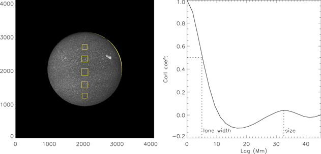
Figure 1. The image and the autocorrelation function. The Kodaikanal Ca ii K image on 1914 Nov 1 and a few representative windows are shown on the left. The autocorrelation curve as a function of lag is shown on the right. The dotted lines give the supergranular lane width and size.
Download figure:
Standard image High-resolution image3. Results
The positive correlation between the lane width and the sunspot cycle is understood as due to the availability of excess magnetic flux at the network boundary as the cycle progresses (Howard 1994). Here, we examine the relationship between the lane widths and the amplitude of sunspot cycles at different epochs. We obtained the lane width during the solar minimum years at different latitudes and correlated it with the maximum of the following sunspot cycle. This is shown in Figure 2 where the lane widths are plotted against the maximum sunspot number for nine different latitudes. The error bars are the standard error of the mean of lane width measurements, which is 0.06 Mm. It can be seen that the correlation is generally good and is highly significant in some latitudes. A straight-line fit is also given, which shows that there is a linear relationship between the two quantities. There is a data gap in 1964, so there are only eight data points.
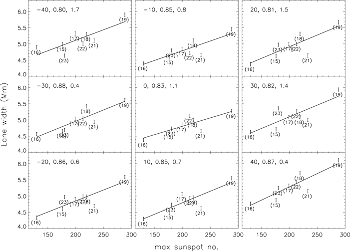
Figure 2. Plots of supergranular lane width during the sunspot minima years vs. maximum sunspot number of the following solar cycle. The latitude, correlation coefficient, and percentage probability that the correlation coefficient arises from two random distributions are mentioned in each plot. A probability ≤1 is considered highly significant (99% confidence level). The continuous line represents a straight-line fit. The error bar and the sunspot cycle number are given at every data point. sunspot data from the World Data Center SILSO, Royal Observatory of Belgium, Brussels.
Download figure:
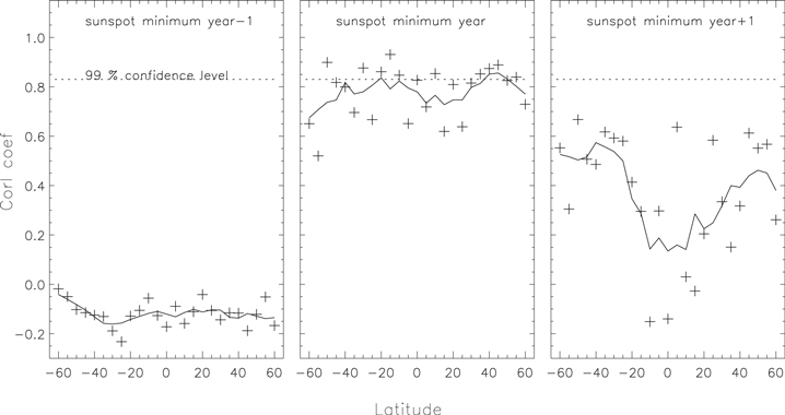
Standard image High-resolution imageNext, we compared the correlation coefficients between the lane width and the maximum sunspot number for three different epochs. We selected a year before the sunspot minimum, the sunspot minimum year, and a year after the sunspot minimum. We obtained the correlation coefficient in all the latitudes. This is shown in Figure 3 where the correlation coefficients are plotted against the solar latitude. A five-point boxcar smoothed curve is also shown to see the average behavior. In the first epoch, which represents the last phase of the previous sunspot cycle, correlations are negligible. In the second epoch, which represents the sunspot minimum year, correlations are maximum and highly significant in some latitudes, especially near the mid-latitudes. Correlation coefficients vary from 0.52 to 0.93 with uncertainties around 18% and 0.0%, respectively. The scatter is more and the peak is not well-defined in the southern hemisphere as compared to the northern hemisphere. The reason for this asymmetry is not clear. The correlations are lower in the third epoch, which represents the initial rising phase of the same sunspot cycle. This shows that the lane widths in the sunspot minimum years are more related to the following sunspot number maxima.
Figure 3. Plots of correlation coefficient between supergranular lane width and the sunspot number maximum vs. solar latitude for three epochs. The panels represent a year before the solar minimum, the solar minimum year, and a year after the solar minimum. The dotted line gives the 99% confidence level. The continuous line represents a smoothed curve. The data are provided in a machine-readable format as the data behind the Figure; it is also accessible from Harvard Dataverse, doi:10.7910/DVN/IRN90W. (The data used to create this figure are available.)
Download figure:
Standard image High-resolution image
The above result is interesting and a bit complex. It shows that supergranular lane widths in the solar minimum year are the indicators of the upcoming maximum sunspot number. However, at other times, the relationship between the lane widths and the maximum sunspot number becomes weaker. These findings point out that the existence of activity has some role in the length scales of large convective cells. During the short period of minimum phase, the length scale of supergranules shows some signs of the amplitude of the upcoming solar cycle. But as soon as the active phase of the next solar cycle begins, this signature weakens. Singh & Bappu (1981) have found that the size of the Ca–K network cell varies with the phase of the solar cycle and is smaller by about 5% during the maximum phase of the cycle. They interpreted this due to the spread of the remnant magnetic field of the decaying plages. This may be due to the generation of small-scale magnetic fields inside the Sun itself. Singh et al. (2023) found that small-scale magnetic fields vary with the phase of the solar cycle using Ca–K images as a proxy. They found that the area of the small-scale magnetic features increases from 5% during the solar minimum phase to 20% during the maximum. We need further theoretical studies to understand the result.
The strong correlation between the supergranular length scale in the sunspot minimum year and the following maximum sunspot number can have some practical applications. It can be used to predict the maximum sunspot number about 4–5 yr in advance. We cannot predict the sunspot number for cycle 25 as the data from Kodaikanal are not available. We have performed a prediction test instead. Note that the correlations in Figure 2 are affected by the two extreme points, hence it is important to know the uncertainty in the prediction. We calculated the correlation coefficients using the combination of six of the eight sunspot cycles and then predicted the sunspot maximum of the remaining two cycles and the uncertainty. This is done eight choose six times (by calculating the binomial coefficient C(8, 6) = 28). A computer program was developed to do these calculations. The results show that one can predict the sunspot maxima of the two cycles with an average uncertainty of about 5.6.
Petrovay (2020) gives a review of solar cycle prediction methods. The precursor method uses the value of some measure of solar activity at a specified time to predict the amplitude of the following solar maximum. Other methods include complex dynamo models and extrapolations. Schatten et al. (1978) suggested the use of polar magnetic field strength around the sunspot minimum as a precursor of the amplitude of the next activity cycle. Proxies of the polar field were reviewed by Petrie et al. (2014). Polar faculae are considered as the best proxy for the polar magnetic field. Three sources of polar facular data are (i) Mt. Wilson Observatory (Petrie et al. 2014), (ii) National Astronomical Observatory of Japan at Mitaka Observatory (Li et al. 2002), and (iii) Kodaikanal Observatory Ca K spectroheliograms (Priyal et al. 2014). The latter data is used by us, so any possible connection between length scales and polar field strength can be studied. In addition to polar faculae, Makarov et al. (2001) reconstructed the polar field strength from Hα data.
A simple measurement of supergranular lane widths during the sunspot minimum provides an easier way to predict the amplitude of the following sunspot cycle. Figure 2 suggests a linear relationship between the measured lane width during the sunspot minimum and the following maximum sunspot number. A straight-line fit in the form y = a0 + a1x, where x is the maximum sunspot number and y is the lane width, yields the coefficients a0 = 3.566 and a1 = 0.007 at latitude 30 S. If the measured lane width is 5 ± 0.06 Mm, a simple rearrangement of the equation yields the maximum sunspot number as 206 ± 7.6. Note that the uncertainty is comparable to those obtained from the prediction test. The results are important in space weather predictions and solar irradiance variations.
Acknowledgments
This work is funded by the Department of Science and Technology, Government of India. We thank the numerous observers and the digitization team of Kodaikanal Solar Observatory for the availability of the data.