


Abstract
Coronal mass ejections (CMEs) are energetic eruptions of organized magnetic structures from the Sun. Therefore, the reconnection of the magnetic field during ejection can excite periodic speed oscillations of CMEs. A previous study showed that speed oscillations are frequently associated with CME propagation. The Solar and Heliospheric Observatory mission's white-light coronagraphs have observed about 30,000 CMEs from 1996 January to the end of 2019 December. This period of time covers two solar cycles (23 and 24). In the present study, the basic attributes of speed oscillations during this period of time were analyzed. We showed that the oscillation parameters (period and amplitude) significantly depend not only on the phase of a given solar cycle but also on the intensity of individual cycles as well. This reveals that the basic attributes of speed oscillation are closely related to the physical conditions prevailing inside the CMEs as well as in the interplanetary medium in which they propagate. Using this approximation, we estimated that, on average, the CME internal magnetic field varies from 18 up to 25 mG between minimum and maximum solar activity. The obtained results show that a detailed analysis of speed oscillations can be a very efficient tool for studying not only the physical properties of the ejections themselves but also the condition of the interplanetary medium in which they expand. This creates completely new perspectives for studying the physical parameters of CMEs shortly after their eruption in the Sun's environment (space seismology).
Export citation and abstract BibTeX RIS

Original content from this work may be used under the terms of the Creative Commons Attribution 4.0 licence. Any further distribution of this work must maintain attribution to the author(s) and the title of the work, journal citation and DOI.
1. Introduction
Coronal mass ejections (CMEs) are energetic expulsions of organized magnetized plasma from the Sun. They are intensively studied because of their significant impact on Earth. The first CME was discovered in 1971 using the seventh Orbiting Solar Observatory (OSO-7) coronagraph (Tousey 1973). Since that time, several space-borne coronagraphs have been observing CMEs (see Gopalswamy 2016 for an overview of the historical development of the field). However, the longest series of observations have been carried out by the Large Angle and Spectrometric Coronagraph (Brueckner et al 1995) on board the Solar and Heliospheric Observatory (SOHO) mission (Domingo et al 1995). The SOHO/Large Angle and Spectromeric Coronagraph Experiment (LASCO) observations covered two solar cycles, numbers 23 and 24. The number of CMEs observed by the SOHO/LASCO coronagraphs was about 30,000 by 2019 December. The observed and derived kinematic properties of all the CMEs are stored among others in the SOHO/LASCO catalog (Yashiro et al 2004; Gopalswamy et al 2009). These data have been analyzed in many studies (Howard et al 1997; Cyr et al 2000; Gopalswamy et al 2003a, 2003b, 2004; Yashiro et al 2004; Gopalswamy 2010). This is the only database created based on manual measurements.
Unfortunately, CME kinematic parameters do not allow us to accurately predict the intensity of geomagnetic disturbances. Now we know that the magnetic field in CMEs and in the sheath ahead of shock-driving CMEs, especially the strength of the magnetic field component oriented in the direction opposite to that of Earth's horizontal magnetic field (Bz ), is crucial in causing geomagnetic storms along with the speed (V) with which the CME hits Earth's magnetosphere (e.g., Wu & Lepping 2002; Gopalswamy et al 2008, 2010b). Routine measurements of magnetic fields in the outer solar atmosphere, where CMEs originate, are not available (Tomczyk et al 2016). To determine the magnetic field in the solar corona, we must apply indirect methods. It seems that one such method may be based on oscillations in the speed of CME. CMEs have an organized flux-rope magnetic structure (Chen 1989; Cargill et al 1994); therefore, the reconnection of the magnetic field during ejection may excite periodic speed oscillations. Periodic speed and intensity oscillations are well established in the case of quiescent prominences, which in many cases are progenitors of CMEs (e.g., Joarder et al 1997). These oscillations have a range of periodicity from a few minutes up to the order of an hour. Krall et al. (2001) first reported the detection of quasi-periodic oscillations in the speed of several CMEs. Shanmugaraju et al. (2010) carefully considered 116 CMEs with at least 10 height–time measurements in the LASCO field of view. They recognized 15 CMEs exhibiting clear quasi-periodic patterns in speed–distance profiles. The amplitudes of oscillations were in the range 157–418 km s−1 and the periods in the range 48–240 minutes, tending to increase with height. The shorter-period, 24–48 minutes, radial and azimuthal oscillations in full halo CMEs were observed by Lee et al. (2015, 2018). Performing two-dimensional numerical MHD simulations of magnetic flux-rope eruption, Takahashi et al. (2017) recorded this kind of oscillation at both the flux-rope bottom and flare-loop top.
Recently, Michalek et al (2016) considered a set of 3463 CMEs during the period of 1996–2004 for which at least 11 height–time measurements were available (10 speed–time points). Using an automatic fitting procedure, they recognized that 22% of the considered CMEs revealed periodic speed fluctuations. The space and time period of the oscillations were in the range from 0.94R⊙/90 minutes (R⊙ is the solar radius) up to 15.97R⊙/824 minutes, respectively. This means that speed oscillation is a frequent phenomenon associated with CME propagation. The nature of speed oscillations was interpreted in terms of normal modes of oscillation of a stretched magnetic string of nonuniform density.
In this paper, we continue these considerations, employing the same fitting procedure and CMEs recorded during the two last solar cycles. The current study covers two complete cycles of solar activity (cycles 23 and 24). The main focus of this research is to show that the speed oscillations of CMEs are a real phenomenon and are significantly related to the changing physical properties of CMEs recorded in different phases of solar activity. This may open up new possibilities in the study of physical conditions prevailing inside the CMEs and in the interplanetary medium in which they propagate.
This paper is organized as follows. In Section 2, the method used for this study is described. The results of our analysis are presented in Section 3. Finally, discussion and conclusions are included in Section 4.
2. Method
In our study of CMEs, we utilized the Coordinate Data Analysis Workshop (CDAW) database (Yashiro et al 2004; Gopalswamy et al 2009). This database consists of a catalog of CMEs with their height–time measurements compiled using manual identification in the LASCO C2 and C3 coronagraph images. We consider a large sample of CMEs detected by the LASCO coronagraphs from 1996 January to 2019 December (about 30,000 of CMEs). This period covers two cycles of solar activity. It is very important because it gives us the opportunity to study the speed oscillations in different periods of solar activity and in different solar cycles.
In the current analysis, to determine the parameters of speed oscillations, we employed the same method that was used in our previous study (Michalek et al 2016). Therefore, in the present paper, we describe this method only briefly. Our procedure has two steps. First, using the CDAW database, from two successive height–time points, speed profiles (instantaneous speeds) for all the considered CMEs are determined (Equation (1) in Michalek et al 2016). Next, a general sinusoidal function, including five free parameters, is fitted to these speed–time profiles. The function has the form (Michalek et al 2016)

where a0 is the amplitude of oscillations, a1 is the frequency of oscillations, a2 is the phase, a3 is the starting speed, and a4 is the acceleration. In the present study we concentrate on the amplitude (a0 ) and the period of oscillations (a1 ). Due to the limited cadence of height–time measurements, we must impose a restriction on the minimum period of oscillations. We assume that the oscillation period cannot be less than 60 minutes. This restriction is due to the time cadence of LASCO observations. Without this restriction, the sinusoidal matching procedure is likely to give completely wrong results. In addition, to be sure of the quality of our fitting procedure, we considered only the events having at least 11 height–time measurements (at least 10 speed–time points). Hence, the fastest CMEs (with speed >1500 km s−1) are not suitable for our oscillation considerations because they have only a few height–time measurements within the LASCO field of view. For the numerical fitting procedure, an Interactive Data Language routine-mpfitfun.pro and Monte Carlo simulations were utilized (to choose the starting parameters). mpfitfun.pro is a nonlinear routine based on the least-squares fitting method (Markwardt 2009). We employed a well-tested procedure that was used in a previous work (Michalek et al 2016). The described procedure was applied to all the CMEs. The initial parameters in the simulations were selected randomly (using the Monte Carlo method). Therefore, in the absence of signs of oscillation, the method we use would simply match a straight line. In Figure 1, two examples of CMEs with fitted curves (dashed lines) to speed–distance/time profiles are presented. In the case of the first CME (left panels), we observe a clear speed oscillation with an amplitude of about 250 km s−1. The other CME (right panels) shows no speed oscillation. In this case, the best fit is a linear function. This shows that the proposed model and the method of fitting the model parameters are correct. The fitting procedure does not rule out a linear fit, i.e., a situation where we do not observe speed oscillations.
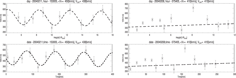
Figure 1. Examples of fitted curves (dashed lines) to speed–distance/time profiles for two CMEs. The left panels show a CME on 2004 February 11, and the right panels show a CME on 2004 February 8, respectively. The upper panels display speed–distance profiles and the lower panels speed–time profiles. In the case of the first CME (left panels), we observe a clear speed oscillation with an amplitude of about 250 m s−1. The other CME (right panels) shows no speed oscillation. In this case, the best fit is a linear function. Error bars show the minimum speed error for the C2 and C3 instruments.
Download figure:
Standard image High-resolution imageOnly after the simulation was completed did we carry out a simple verification of the obtained parameters. During this verification, doubtful events were rejected. First, we assumed that the simulation result is reliable when the oscillation amplitude is higher than 30 km s−1 or 15% of the average speed, whichever higher. These limits were adopted on the basis of research specifying errors in determining height–time points resulting from the manual measurements used for the construction of the catalog (Shanmugaraju et al 2010; Michalek et al 2017). These flexible limits allowed us not to reject, from further considerations, slow CMEs. We also assumed that the upper limit in amplitude is 400 km s−1. This limit is to avoid situations where the amplitude of oscillations is larger than the actual speed of an event. Additionally, we assumed that the time period of oscillations is less than 850 minutes. This limit is due to due to the limited LASCO field of view (limited time of observation for a given event). It should also be mentioned that according to Michalek et al (2016), the vast majority of CMEs have very small fitting errors. The average value of the relative errors of the amplitudes of oscillations (error in determining the amplitude to the amplitude value) was 0.07.
3. Results
In the considered period of time (1996–2019), we obtained a large sample of CMEs (3893) showing periodic oscillations in speeds. This is 13% of all the recorded CMEs (or 22% of CMEs having at least 11 height–time measurements). The same results were obtained by Michalek et al (2016).
3.1. General Properties of Speed Oscillations and CMEs
The distributions of the most important attributes of oscillations and CMEs revealing speed oscillations are displayed in Figure 1. The left panels (Figures 2(a)–(d)) show the distributions of the basic attributes of oscillations (amplitude, space period, time period, and acceleration). The spatial periods were calculated from the time periods using speeds of CMEs. The right panels display the distributions of speeds, widths, absolute latitudes, and accelerations of CMEs revealing these oscillations. The CME parameters are from the CDAW database. The amplitudes of oscillations could be very significant up to 395 km s−1. The average amplitude of oscillations is 93 km s−1, which is about 20% of the average ejection speed. This means that oscillations are a pronounced phenomenon. Periods of oscillations range from 90 to 829 minutes. The bottom left panel in Figure 2 displays the acceleration evaluated on the basis of the speed–distance profiles (parameter a4 in Equation (1)). It is different from the acceleration obtained by second-order fitting to the height–time plots reported in the SOHO/LASCO catalog. CMEs revealing an oscillation pattern mostly move with constant speeds in the LASCO field of view. Oscillation parameters obtained in the current simulations are consistent with the results of previous studies (Shanmugaraju et al 2010; Michalek et al 2016).

Figure 2. Distributions of the most important attributes of speed oscillations (left panels, a–d) and CMEs revealing these oscillations (right panels, e–h). In the left panels are the distributions of (a) the amplitude of oscillation (parameter a0), (b) spatial period of oscillation (obtained from time period oscillation), (c) time period of oscillation (parameter a1), and (d) acceleration (parameter a4). Basic statistics (mean, median, and standard deviation) are reported at the top of the panels. In the right panels are the distributions of (e) speed, (f) width, (g) absolute latitude, and (h) acceleration of CMEs revealing speed oscillations. The fraction is the ratio of the number of CMEs with the given parameters falling within the ranges under consideration to all CMEs with an oscillation pattern.
Download figure:
Standard image High-resolution imageThe CMEs' attributes (Figures 2(e)–(h)) cover wide ranges of values (87–1352 km s−1 for speed, 3°–314° for angular width (not including halos), 0°–90° for absolute latitudes, and −81 to +90 m s−2 for acceleration) implying that the speed oscillation is a feature associated with various classes of events. The distributions of CME attributes revealing oscillations are very similar to those obtained for the general populations of CMEs (Yashiro et al 2004). Only the speed of oscillating CMEs seems to be on average smaller in comparison with the average speed of the general population of CMEs. This difference is caused by our selection criteria (there should be 11 height–time measurements), which excluded from our study fast CMEs because the number of their height–time points is less than 11.
3.2. Oscillation Appearance Frequency
Figure 3 shows the temporal evolution of the occurrence rate of CMEs with oscillation patterns. The most frequent oscillations were recorded during the maximum phase of solar cycle (SC) 24 (2013). During this period, about 350 CMEs per year revealed speed oscillations, two times more than in SC 23. This is an intriguing result because according to the sunspot number (SSN), SC 24 was weaker than SC 23. It seems to be the result of two effects. First of all, during SC 24, many more ejections were recorded compared to the SC 23 (Michalek et al 2016). Furthermore, the cadence of LASCO observations was doubled in 2010. This allowed us to observe the CMEs with a higher time resolution, which significantly increased the ejection sample having at least 11 height–time measurements. However, it should be noted that the high detection rate was maintained from the maximum of SC 23 even during the minimum of solar activity between both cycles. The fractional detection rate (Figure 3, bottom panel) behaves a little differently in comparison to the occurrence rate of CMEs (top panel). An increase in this parameter occurred in 2004 and reached its maximum in 2010 (about 0.2) (in the initial phase of growth of solar activity in cycle 24). This means that this increase was not caused by a change in the time cadence of LASCO observations.

Figure 3. Temporal evolution of the occurrence rate of CMEs showing an oscillation pattern: (a) the absolute and (b) fractional occurrence rates (the ratio of CMEs with an oscillation pattern to the total number of CMEs in a given period of time).
Download figure:
Standard image High-resolution image3.3. Oscillation during the Last Two Solar Activity Cycles
Having observations over a period of two cycles of solar activity, the most intriguing question is to study the parameters of oscillation in different phases of solar activity. Figure 4 shows the temporal evolution of the average annual values of the solar spot number (SSN; panel a), speed of CMEs revealing oscillations (panel b), periods of oscillations (panel c), and their amplitudes (panel d). The results presented in this figure are the most important new achievements of the research carried out. The most striking feature is that all the considered parameters follow cycles of solar activity. This confirms that speed oscillations are a real phenomenon that depends on the current physical conditions prevailing in the Sun. Table 1 displays the linear Pearson (Spearman's rank) correlation coefficients for the considered parameters. We performed a test of the significance of the correlation coefficients. For the Pearson correlation coefficient, at the significance level α = 0.05, there is sufficient evidence to conclude that there is a significant linear relation between these parameters. This means that these indicators are significantly related to solar activity cycles and also to each other. This result is obviously not new or surprising in the case of CME speeds (e.g., Yashiro et al 2004). We know that during a solar maximum, the CMEs are more energetic because then more magnetic energy is involved in their ejection. A completely new and very promising result was obtained for the oscillation parameters. The oscillation periods are clearly anticorrelated with CME speeds and SSNs. In the maxima of solar activity, on average, periods of pulsation are ≈240 minutes and in minima as much as ≈300 minutes. This means that periods of oscillations depend on the physical properties of ejections. It is assumed (Michalek et al 2016) that the flux-rope structure inside CMEs can be approximated as a stretched elastic string of nonuniform density (Leroy 1989; Ruždjak & Tandberg-Hanssen 1989). Then, periods of string mode oscillation can be expressed as (Roberts 1991)

where a is the half-width of the prominence, l is half the length of the flux-rope string, and CA is the speed of MHD waves. This means that for a given flux-rope size, a smaller CA can result in a larger P. Assuming typical parameters of coronal plasma and CMEs at distance 5R⊙ (n = 1.6 × 10⁴ [cm−3], l = 5R⊙), and a is 60 times less than l (as is the radius of the cross section), we can derive, on the basis of period fluctuation (300 and 240 minutes), that on average the internal magnetic field of CMEs varies from 18 up to 25 mG between minimum and maximum of solar activity. Using the dispersion for all determined periods of oscillation and standard methods for determining measurement uncertainties (the law of uncertainty propagation for a function of one argument), we obtained an error in determining the magnetic field equal to 2 mG. This means that the relative error in determining the magnetic field is on the order of 10%. However, it is necessary to note that this error was determined on the basis of the conducted considerations. However, there is an uncertainty in the determination of the magnetic field resulting from the assumptions employed. Equation (2) assumes a simplified shape of the magnetic field. We know that in reality, the magnetic field carried by CMEs is a very complicated and strongly twisted—the flux-rope structure. This means that the determined magnetic field can be overestimated. We are currently unable to include this effect in our research. Similar values of magnetic fields included in the CMEs at a distance of 10R⊙ were obtained by Gopalswamy et al (2018) (they computed the total reconnection flux involved in each of the solar eruptions). These results show that the physical parameters of CMEs can be inferred by analyzing their speed oscillations. Another parameter describing oscillations is amplitude. It is also correlated with solar activity. It ranges from 60 km s−1 to 110 km s−1 depending on the phase of the cycles (Figure 4(d)). In periods of minimum solar activity, it is lower and in periods of maximum activity, it clearly increases. It behaves similarly to the speed of CMEs. The amplitude of oscillations is larger during maxima of solar cycles where CMEs are more energetic. But, there is one intriguing thing about amplitude. It can be clearly seen that during the maximum of SC 24, the average oscillation amplitude was significantly higher than that during the maximum of cycle 23 (about 20%), despite the fact that the average speeds of CMEs behave inversely. It would seem that more energetic (faster) bursts should generate higher oscillation amplitudes. However, the amplitudes behave differently. One guess is that the oscillation amplitudes depend not only on the internal parameters of the CMEs but also on the conditions prevailing in the interplanetary medium. We know that after the exceptionally extended and low levels of solar activity between cycles 23 and 24, the interplanetary medium became an extremely rare field (Gopalswamy et al 2014, 2015). The drag force caused by the interplanetary medium is mainly responsible for the suppression of oscillations. Therefore, during this period, when the interplanetary medium was extremely rare, the oscillations could develop freely and reach high amplitudes. This can also explain the large number of oscillating CMEs recorded during this period of time.

Figure 4. Temporal evolution of average annual values of solar spot numbers (panel a), speed of CMEs revealing oscillations (panel b), periods of oscillations (panel c), and their amplitudes (panel d). Error bars show the standard deviation for a given sample. Dashed lines in panels (c) and (d) represent the results obtained with a reduced cadence of height–time points to match the SC 23 cadence.
Download figure:
Standard image High-resolution image
Table 1. Correlation Coefficients: Pearson and Spearman's Rank (in Brackets)
| SSN | Speed of CMEs | Period of Oscillations | Amplitude of Oscillations | |
|---|---|---|---|---|
| SSN | 1(1) | 0.91(0.92) | −0.54(−0.56) | 0.44(0.54) |
| Speed of CMEs | 0.91(0.92) | 1(1) | −0.63(−0.61) | 0.50(0.58) |
| Period of oscillations | −0.54(−0.56) | −0.63(−0.61) | 1(1) | −0.87(−0.88) |
| Amplitude of oscillations | 0.44(0.54) | 0.50(0.58) | −0.87(−0.88) | 1(1) |
Download table as: ASCIITypeset image
However, before drawing any final conclusions, we must pay attention to the fact that in 2010 August, the LASCO image cadence increased from 60 images per day to about 100 images per day (e.g., Wang & Colaninno 2014). Therefore, it is necessary to check if the cadence change could affect our assumptions. For this purpose, we carried out our simulations with a reduced cadence of height–time points to match the SC 23 cadence. The results of these simulations are presented in Figure 4 (for the period and amplitude of oscillations, panels (c) and (d), respectively) as dashed lines. The presented curves show that the change in cadence did not significantly affect the oscillation parameters. Only in the case of the oscillation period did we observe that the reduction of the cadence caused, on average, a decrease in the oscillation period by 10%. This result is not surprising as the decrease in the sampling frequency must cause a decrease in the detection rate of oscillations with lower periods. In the case of the oscillation amplitude, the cadence reduction has no effect on the simulation results. Within the error limits, both curves practically coincide. The test simulations carried out also confirm that the method used to analyze the oscillations does not depend on the cadence of observations, and the obtained results reveal real variations in the speed of CMEs during their expansion in the LASCO field of view.
It seems that a detailed analysis of oscillations will allow, in the future, not only the physical properties of the ejections themselves but also the condition of interplanetary medium in which they expand to be studied.
4. Conclusions
We considered all the CMEs with at least 11 height–time measurements included in the CDAW database in the period of 1996–2019. It allowed us to evaluate speed–time profiles with enough accuracy to analyze oscillations in the speed of CMEs. Of the considered CMEs, 22% revealed periodic speed fluctuations during their expansion in the interplanetary medium. This means that speed oscillation is a frequent phenomenon associated with CME propagation. Distributions of basic attributes of speed oscillation are similar to those obtained previously (Shanmugaraju et al 2010; Michalek et al 2016). We have obtained the following new important results.
We demonstrated that the average values of the basic attributes of oscillations (amplitude and period) are significantly correlated with cycles of solar activity.
In the maxima of solar activity, on average, pulsation periods are ≈240 minutes and in minima as much as ≈300 minutes. This means that periods of oscillations depend on the physical properties of ejections. It is assumed (Michalek et al 2016) that the flux-rope structure inside CMEs can be approximated as a stretched elastic string of nonuniform density. Using this approximation, we estimated that, on average, the CME internal magnetic field varies from 18 up to 25 mG between the minimum and maximum of solar activity.
We also recognized that the average amplitude of oscillation also varies with solar cycle (from 60 up to 110 km s−1; Figure 4(d)). In addition, we revealed that during the maximum of cycle 24, the average oscillation amplitude was significantly higher than that during the maximum of cycle 23 (about 20%), despite the fact that the average speeds of the CMEs behave inversely. We suppose that these intriguing results are due to an anomalous physical condition during the last cycle. Due to the significant decline in solar activity during the last minimum of solar activity, the interplanetary medium became extremely rare. Hence, drag force, which should suppress oscillations, was also very weak. Then, oscillations could develop freely and reach high amplitudes. This can also explain the large number of oscillations recorded during this period of time.
The test simulations with the reduced cadence of LASCO images demonstrated that the presented result revealed real variations of CMEs in the LASCO field of view.
The obtained results show that a detailed analysis of speed oscillations can be a very efficient tool for studying not only the physical properties of the ejections themselves but also the condition of the interplanetary medium in which they expand.
We would like to thank the reviewer for substantive comments and constructive cooperation during the correction of the article. This work was supported by NASA's LWS program.