


Abstract
While low-frequency plasma fluctuations in the interplanetary space have been successfully described in the framework of classical turbulence, high-frequency fluctuations still represent a challenge for theoretical models. At these scales, kinetic plasma processes are at work, but although some of them have been identified in spacecraft measurements, their global effects on observable quantities are sometimes not fully understood. In this paper we present a new framework to the aim of describing the observed magnetic energy spectrum and directly identify in the data the presence of Landau damping as the main collisionless dissipative process in the solar wind.
Export citation and abstract BibTeX RIS

Original content from this work may be used under the terms of the Creative Commons Attribution 4.0 licence. Any further distribution of this work must maintain attribution to the author(s) and the title of the work, journal citation and DOI.
1. Introduction
Nonlinear interactions and turbulence play a key role in determining the evolution of several astrophysical plasma systems (Coleman 1968; Scalo & Elmegreen 2004; Zhuravleva et al. 2014; Cranmer et al. 2015; Bruno & Carbone 2016). In such cases, energy is injected at large scales and cascades to microscales where it is finally dissipated, thus heating the medium. However, due to the very weak collisionality of astrophysical plasmas, identifying the physical mechanism that replaces viscosity for efficient energy dissipation and heating is still a challenge for theoretical models (Goldstein et al. 2015; Chen 2016; Boldyrev et al. 2020). Due to its proximity to the Earth, the Solar Wind, namely the collisionless plasma coming from the expanding solar corona which pervades the interplanetary space, represents a unique natural laboratory to study turbulence and all the microphysical plasma processes related to the transfer of energy from the turbulent electromagnetic field to the plasma particles (Goldstein et al. 2015; Bruno & Carbone 2016; Chen 2016). In situ spacecraft can directly probe the interplanetary plasma, thus providing high-resolution measurements (Goldstein et al. 2015; Bruno & Carbone 2016; Chen 2016).
The first evidence for the presence of turbulence in the interplanetary space was provided by space missions during the 1960s (Coleman 1968) and it is nowadays agreed that fluctuations at frequencies below the ionic break fb
, roughly found in the range 0.1 ≤ fb
≤ 1 Hz, are produced by a turbulent nonlinear energy cascade (Sorriso-Valvo et al. 2007; MacBride et al. 2008; Carbone et al. 2009; Banerjee et al. 2016; Bruno & Carbone 2016). The magnetic energy spectrum scaling observed in the frequency domain ω is in good agreement with the Kolmogorov law E(k) ∼ k−5/3 (Bruno & Carbone 2016) once frequencies are transformed in wave vectors k by using the Taylor hypothesis. The cascade transfers energy beyond the ionic break, that is, in the dispersive-dissipative range, where the scale-free magnetic energy Kolmogorov spectrum breaks down (Leamon et al. 1998) and the magnetic fluctuations are described by a steeper power law E(ω) ≃ ω−α
which covers more or less two frequency decades up to about 100 Hz, with a scaling exponent ranging in the interval 2 ≤ α ≤ 4, roughly centered in the range  (Alexandrova et al. 2009; Sahraoui et al. 2009; Goldstein et al. 2015). The observed nonuniversality of the scaling exponents suggests the presence of some different nonlinear wave–wave coupling kinetic mechanisms. The process of quasi-two-dimensional nonlinear interactions of kinetic Alfvén waves (Leamon et al. 1998; Bale et al. 2005; Sahraoui et al. 2009, 2010; Salem et al. 2012; Chen et al. 2013; Kiyani et al. 2013; Podesta 2013; Roberts et al. 2013), for which E(ω) ≃ ω−7/3, is the most supported one in the literature (Cho & Lazarian 2004; Schekochihin et al. 2009) provided that the linear damping rate is zero and that no intermittency corrections are included, but other interpretations involve other mode couplings, such as magnetosonic Whistler (Gary & Smith 2009; Narita et al. 2011, 2016), kinetic slow modes (Yao et al. 2011; Howes et al. 2012), and ion Bernstein modes (Perschke et al. 2013). For example, intermittency steepens the spectrum to E(ω) ≃ ω−8/3 (Boldyrev & Perez 2012), and Landau/Barnes damping can steepen it to a value that is parameter-dependent (Howes et al. 2011; TenBarge et al. 2013; Kawazura et al. 2019). A clear unambiguous recognition of wave modes of a single type in the frequency wave-number diagram is impossible due to the presence of large scattering, sideband modes, sporadic wave trains as envelope solitons, and zero-frequency modes (Narita et al. 2011; Perschke et al. 2016). At most, it can be concluded that kinetic modes, to a different extent, could contribute to nonlinear couplings, being subject, at the same time, to dispersive and dissipative effects (Gary & Smith 2009).
The electronic break is observed at a frequency of about 100 Hz, and beyond this break magnetic fluctuations have been described either through a further power law (Sahraoui et al. 2009) E(ω) ≃ ω−σ (where σ ranges in the interval 3.5 ≤ σ ≤5.5) or by means of an exponential decay (Alexandrova et al. 2012). Observations, limited to a range covering a few hundred Hz, cannot provide a clear indication (Goldstein et al. 2015). This range of frequencies has been interpreted as a region where collisionless dissipative mechanisms are efficiently at work (Sahraoui et al. 2009; Alexandrova et al. 2012; Goldstein et al. 2015). However, the nature of these mechanisms is strongly debated. The processes proposed in the literature include ion–cyclotron damping (Coleman 1968; Smith et al. 2012), Landau damping (Howes et al. 2008; TenBarge & Howes 2013), stochastic heating (Chandran 2010), entropy cascade (Schekochihin et al. 2009), and magnetic reconnection (Egedal et al. 2012; Drake & Swisdak 2014), most of them already being active at ion scales, and/or between the ion and electron scale. Recently, direct signatures consistent with the presence of Landau damping have been found in the Earth's magnetosphere (Chen et al. 2019).
Beyond the ion gyro-radius or the inertial length, which at 1 au are unfortunately of the same order of magnitude, the plasma dynamics becomes extremely complex. More specifically, many different characteristic plasma microscales appear and the linear wave modes become kinetic, thus exhibiting at the same time both a dispersive and a dissipative character, due to wave–wave and wave–particle interactions. In a range of scales where dispersive effects, wave–wave couplings, collisionless dissipation, and plasma heating take place and the presence of characteristic frequencies breaks down the scale-free behavior, the combined role of dispersion and dissipation of the fluctuations is still poorly understood. Although the physics underlying the dynamics are quite far from classical fluid-like turbulence in which the nonlinear cascade operates within a scale-free range, well separated from the smallest scales where viscous dissipation occurs, microscale fluctuations are sometimes conservatively interpreted in terms of further turbulent cascades, mainly involving wave–wave couplings. While the statistical information obtained at large scales is universal, namely well-defined scaling indices are observed, the scaling of structure functions at small scales showed a break of universality. This prevents the possibility of firmly characterizing fluctuations through an underlying physical process, starting, for example, from a turbulent-like approach. New attempts could, in principle, increase our knowledge on the observed fluctuations. Therefore, in this paper, we use a novel predictive approach to define a framework that allows us to describe the observed magnetic energy spectrum and directly infer from the data the presence of Landau damping as the main collisionless dissipative process in the solar wind.
2. Model and Results
The microscale plasma dynamics involve a plasma where random fluctuations and dissipation cooperate in a complex way, thus resulting in a continuous generation and dissipation of magnetic and electric fluctuations. To describe this medium, let us consider a simple Brownian-like framework where magnetic fluctuations b (t) at small scales can be described by an Itô stochastic differential equation involving two different contributions

The first term on the r.h.s. mimics a collisionless mechanism and can be simply written as Γ[
b
(t), t] ≃ − γ
b
(t), γ being the phenomenological damping rate. The second contribution, which describes all the complex wave dynamics, is described through a stochastic process d
W
(t). For the sake of simplicity, F[
b
(t), t] ≃ F0 is assumed equal to the r.m.s. of the fluctuations F0 = 〈b2〉1/2. The random forcing is expressed as d
W
(t) =
ξ
(t)dt, which is a suitable physical choice for an interpretation of
ξ
(t) as real noise, possibly different from white noise, with finite correlation times (Gardiner 2009). For simplicity, we assume that ξ(t) is uncorrelated with the initial values of the magnetic fluctuations. Equation (1) can easily be solved through a Fourier transform, thus obtaining, for a stationary process, a relation between the correlations of the Fourier magnetic modes
b
ω
and those of the stochastic Fourier modes
ξ
ω
. Taking into account that  , where E(ω) is the magnetic energy density spectrum and
  (being G(ω) the spectrum of the forcing), the following relation is obtained

Stochastic fluctuations generated by the dynamical microphysics of the plasma cannot be described by completely uncorrelated random events. Without loss of generality, let us consider the case where the two-point correlations of the stochastic term decay exponentially in time ![$\langle {\boldsymbol{\xi }}(t)\cdot {\boldsymbol{\xi }}({t}^{{\prime} })\rangle =\exp [-\lambda ({t}^{{\prime} }-t)]$](https://content.cld.iop.org/journals/2041-8205/924/2/L26/revision1/apjlac4740ieqn4.gif) , with relaxation rates λ distributed according to a probability of occurrence
, with relaxation rates λ distributed according to a probability of occurrence  , where λ0 and μ are free positive parameters. In this case, the functional shape of the magnetic density energy spectrum results in

where  is a smooth function of μ and Δ is a typical scale of the exponential decay rate of the stochastic two-point correlations. Assuming Δ ∼ γ, a simple direct numerical estimate gives I(μ) ≃ 0.5–0.13μ.
Relation (3) is able to describe the magnetic density energy spectra obtained from Cluster spacecraft data, as reported in Figure 1. The fit of this function on the data gives us a set of values for the scaling exponent μ and for the dissipation rate γ, whose distributions are reported in Figure 2. The relative errors for the gamma values obtained with the model are mostly in the range of 6%–8%; only very few are above 10%. The good accuracy of the gamma estimation comes from the fact that the model has only 2 free parameters (excluding the normalization factor) related to the slope of the spectrum (μ) and the cut-off (γ), respectively. It is also important to point out that the fact that some of the γ-values are in the frequency range in which Cluster data are severely affected by noise is perfectly fine, as the model is predictive in its nature. This is actually one of the novelties of the proposed model: it can estimate a cut-off at frequencies that are not directly observed, based on measurements at lower frequencies. Moreover, it is worth noting that the model was not built ad hoc to fit the observations.

Figure 1. Examples of magnetic energy density spectra obtained from three different 30 minute long samples selected from the data set of the Cluster spacecraft (the referenced time interval which identifies each sample is reported on the different panels). The fit with relation (3), beyond the ionic break, is shown in red and best-fit parameters are reported on the plots. As a reference, we also plot the power laws ω−5/3 in the inertial range, and ω−(1+μ) beyond the ionic break, respectively. The value of the frequency γ is shown with the green arrows.
Download figure:
Standard image High-resolution image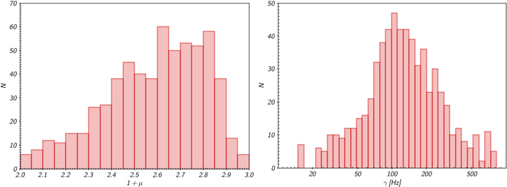
Figure 2. Distributions of 1 + μ (left panel) and γ (right panel) obtained through a fit of Equation (3) to the magnetic energy density spectra obtained from N = 631 samples of the data set of the Cluster spacecraft.
Download figure:
Standard image High-resolution imageThe values of 1 + μ we obtained, roughly centered around 1 + μ ≃ 2.67, correspond to the observed slopes of the power spectra in the ionic frequency range (Sahraoui et al. 2009), while the values of γ, peaked around 100 Hz, result are of the order of the electronic break which has been sometimes observed in high-β solar wind data (Sahraoui et al. 2009). Note that Equation (3) is also compatible with a double power law made by ω−(1+μ) at ionic frequencies ω ≪ γ, and ω−(3+μ) at higher frequencies ω ≫ γ. Both a relation similar to (3) and a double power law have been used as ad hoc functions to fit data in previous works (Sahraoui et al. 2009). Here we show that the observed magnetic energy spectrum at high frequencies can simply be recovered when the microphysical plasma dynamics are assumed to be driven by a stochastic source of fluctuations, without necessarily invoking a further scale-free turbulent cascade (Carbone et al. 2018).
Since measurements are obtained in the spacecraft reference frame, when comparing the power spectra obtained from solar wind observations to those given by our model, we should take into account that there is not a one-to-one correspondence between the plasma-frame and spacecraft-frame frequency spectra. According to the Doppler-shift formula, the measured frequency ωsc (in the spacecraft frame) of a Fourier mode of wave vector k and frequency ω is given by ωsc = ω + k · v SW , where v SW is the solar wind velocity. Two relevant situations can occur in the high frequency range (Klein et al. 2013). When the solar wind speed is slow enough, ∣ω∣ ≳ ∣ k · v SW ∣ and this gives rise to a constant shift of the frequency spectrum to higher frequencies in the spacecraft frame without changes in the scaling of the spectrum (Klein et al. 2013). As a consequence, the scaling predictions of our model should still be valid in this case, the only change being a shift of the high-frequency breakpoint by a constant value Ω0, namely ωe ≈ γ + Ω0. The other relevant case is the dispersive regime, in which the plasma-frame frequency increases more rapidly than linearly and ωsc is eventually dominated by the plasma-frequency term (ωsc ≈ ω). Also in this case, the spectra of our model, being obtained straight in the frequency domain and since ωsc ≈ ω, can be directly compared to those measured by spacecraft.
The physical origin of γ, which is still a parameter in the Langevin model, can be clarified by investigating the statistical properties of the model. To this aim, we need an invariant probability measure on the space of states of the stochastic magnetic variables. This is a long-standing problem in turbulence that has been partially solved by D. Ruelle (Ruelle 1978) who conjectured that the most appropriate distribution, the so-called Sinai–Ruelle–Bowen (SRB) distribution, exists for the nonequilibrium turbulent system (Bowen 1970; Sinai 1977; Ruelle 1980), requiring that the system shows typical characteristics of chaoticity (chaotic hypothesis; Gallavotti & Cohen 1995). The conjecture has been extended to a wide range of nonequilibrium stochastic systems (Gallavotti & Cohen 1995), of course including the Langevin dynamics. For a given observable v, by formally defining the statistical measure Ω(F(v)) on a function of the observable as the limit of time averages of iterates of, for example, a Gibbs distribution μG , the SRB measure can be defined as

where St is the time evolution operator of the dynamics and A is the attracting phase space, namely a usual, smooth-bounded Riemannian compact manifold (Gallavotti & Cohen 1995). The interest of this is the fact that, when the system is conservative, the following limit exists

that is, the time evolution of the system, which has an empirical chaotic nature, implies the ergodic hypothesis. This means that the chaotic hypothesis and the SRB measure generally imply the Onsager reciprocity and the existence of a fluctuation–dissipation relation (Gallavotti 1996b, 1996a) because the virial theorem can be extended to a wide range of out-of-equilibrium systems (Felasco et al. 2016). This allows us to link the statistics of microscopic fluctuations to the properties of macroscopic dissipation since the statistics of the conservative out-of-equilibrium system are equivalent to the statistics of an equilibrium system, as stated by Equation (5).
The theory of equivalence of probability measures between equilibrium and out-of-equilibrium systems is formally true for a time-invariant system rather than for a dissipative system where the phase space is contracting, so that one might introduce a conservative counterpart of the model. To this purpose, following previous approaches on turbulence models (Eckmann & Ruelle 1985; Gallavotti & Cohen 1995; Gallavotti 2014; Gallavotti & Lucarini 2014; Biferale et al. 2018), it is useful to rewrite the model (1) as

where the function α is a stochastic arbitrary function describing the microscopic properties of the dissipation, and ζj are independent chaotic motions. If we define
(μ0 is the vacuum permittivity), Equation (6) has an exact constant of motion  , if the initial data are on the surface Λ, so that the system is time-invariant, independently of initial conditions. As a consequence, the equivalence conjecture indicates that: i) if the initial Λ for Equation (6) is the total energy for Equation (1), the models (1) and (6) are equivalent as far as statistical properties are concerned; ii) the average of α on the SRB probability measure, as, for example, a smooth Gaussian function centered around fluctuations where
  , defines the phase-space contraction rate and is proportional to the damping rate 〈α〉SRB ∼ γ of Equation (1) (Gallavotti & Cohen 1995; Gallavotti 2014).
In this framework, working out our Brownian-like approach, from relation (6) we can obtain an equation for the average magnetic energy density

which depends on the correlations between the magnetic fluctuations and the stochastic forcing term. Equation (8) can be formally solved using relation (1), thus obtaining, after some algebra,
From this last equation, according to the statistical equivalence of the models, a stationary solution for the average magnetic energy density can be found. This solution is finite provided that γ > λ0, and, in general, this is a nonequilibrium stationary solution, that is, for almost all initial conditions the long time evolution of Λ(t) tends to ρ(A, F, Ω) = ∫A F(v)Ω(dv), where F(v) is any function of the observable. After straightforward calculations, we then obtain
where ![$h(\mu )=\left[{\int }_{{\rm{\Delta }}/\gamma }^{\infty }{x}^{-\mu }{\left(x-1\right)}^{-1}{dx}\right]$](https://content.cld.iop.org/journals/2041-8205/924/2/L26/revision1/apjlac4740ieqn9.gif) is a smooth function of μ, and
is a smooth function of μ, and  is the square modulus of the total magnetic field. Assuming Δ ∼ γ, a simple direct numerical estimate gives h(μ) ≃ (6 − μ/3).
The observable F(v) is arbitrary, so that if we are interested in the squared electron plasma-velocity fluctuations, we are free to use F(v) = v2, thus roughly identifying ρ(A, F, Ω) as a stationary nonequilibrium "electron temperature" kB T by using the kinetic velocity-distribution function f(v) in the SRB measure Ω(dv) ∼ f(v)dv. From Equation (10), the phenomenological damping rate turns out to be proportional to some power of the temperature, defined through the second-order electron velocities

Equation (10) can be more appropriately written in terms of the electron plasma-β parameter

where ne
is the electron-number density and  , being
  and
and  the Alfvén and thermal velocities, respectively. Equation (12) represents the fluctuation–dissipation relation (FDR) in our Brownian approach (Kubo 1966; Gallavotti 1996a, 2014), describing the relation between the macroscopic dissipation of the collisionless plasma and its statistical fluctuations. It is worthwhile to note that the presence of the FDR does not necessarily require either a statistical equilibrium involving a maximal entropy or fluctuations described by a Maxwellian distribution (Gallavotti & Cohen 1995; Morrison & Shadwick 2008). From a physical point of view, an FDR based on the fluctuation theorem (Gallavotti 1996b) also can be found in an evolving chaotic system with a given dynamical, statistical SRB distribution of orbits in the phase space (Eckmann & Ruelle 1985; Gallavotti & Cohen 1995; Gallavotti 1996b, 1996a, 2014). The FDR gives information on the fine structure of the attractor. The same happens, for example, in the turbulent cascade and in other nonequilibrium statistical processes (Gallavotti 1996a, 1997, 2014; Gallavotti & Lucarini 2014; Biferale et al. 2018), including fluctuations in non-Maxwellian plasmas described by the Vlasov equation (Morrison & Shadwick 2008).
The FDR is fundamental to identifying the collisionless dissipation mechanism at work in the solar wind. As a simple estimate, when the scaling exponent has the typical observed value, say 1 + μ ≃ 8/3 (Sahraoui et al. 2009), assuming that kB
T is the observed temperature calculated from the second moment of the fluctuations, relation (11) gives the scaling law  which is the classical scaling relation between the damping rate of electron Landau damping and plasma temperature (Alexeev 2004), as well as the scaling relation for the electron collision frequency in plasmas.
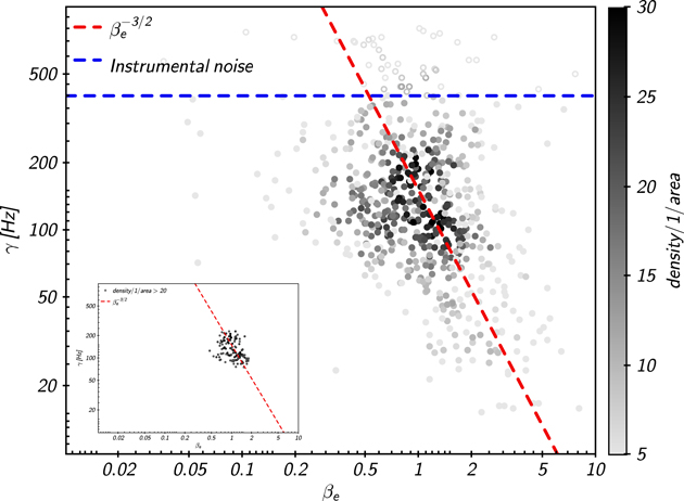
Equation (12) can be verified in the magnetized solar wind plasma. In Figure 3 we report the observed relation between the values of γ, estimated on the data through Equation (3), and the corresponding measured values of βe in the corresponding solar wind data. Points corresponding to γ above (below) the instrumental noise (400 Hz, Alexandrova et al. 2012, indicated by a blue dashed horizontal line in the figure) are marked as open (filled) circles.
Figure 3. Scatter plot of the density of points in the plane (βe
, γ) for the N = 631 samples selected by the data set of the Cluster spacecraft. A power law  is reported as a dashed red line. The 400 Hz noise floor (Alexandrova et al. 2012) is marked by a blue dashed horizontal line: points corresponding to γ values above (below) it are displayed as open (filled) signs. The γ values have been obtained for all samples from best fits of Equation (3). For each γ, the corresponding value of βe
is measured from the parameters of the sample. In the inset figure we plot the plane (βe
, γ) by using only a density of points ≥20.
is reported as a dashed red line. The 400 Hz noise floor (Alexandrova et al. 2012) is marked by a blue dashed horizontal line: points corresponding to γ values above (below) it are displayed as open (filled) signs. The γ values have been obtained for all samples from best fits of Equation (3). For each γ, the corresponding value of βe
is measured from the parameters of the sample. In the inset figure we plot the plane (βe
, γ) by using only a density of points ≥20.
Download figure:
Standard image High-resolution image
A power-law relation  for the dissipation rate, displayed as a reference in the figure, well reproduces the results obtained from solar wind data, which are thus in good agreement with our model (12). This direct relation, underlined for the first time, represents a strong signature to identify the main dissipation mechanism in the solar wind, namely the presence of electron Landau damping, which perhaps represents the main collisionless dissipation mechanism of fluctuations, along with residual dissipation due to collisions. Therefore, we can identify γ in Equation (1) as the average damping rate of the fluctuations, which, according to our findings, turns out to be roughly proportional to the electron break observed sometimes in the solar wind plasma. By using typical values 1 + μ ≃ 8/3, ne
≃ 3 cm−3 and βe
≃ 0.7 (Sahraoui et al. 2009), stochastic fluctuations at the scale Δ ∼ γ gives (γ/λ0) ≃ 102, which is a typical estimated value for the separation between the ionic and electron spectral breaks in the solar wind β ≃ 1 plasma (Sahraoui et al. 2009; Goldstein et al. 2015). This allows us to identify λ0 to be of the order of the ionic break.
for the dissipation rate, displayed as a reference in the figure, well reproduces the results obtained from solar wind data, which are thus in good agreement with our model (12). This direct relation, underlined for the first time, represents a strong signature to identify the main dissipation mechanism in the solar wind, namely the presence of electron Landau damping, which perhaps represents the main collisionless dissipation mechanism of fluctuations, along with residual dissipation due to collisions. Therefore, we can identify γ in Equation (1) as the average damping rate of the fluctuations, which, according to our findings, turns out to be roughly proportional to the electron break observed sometimes in the solar wind plasma. By using typical values 1 + μ ≃ 8/3, ne
≃ 3 cm−3 and βe
≃ 0.7 (Sahraoui et al. 2009), stochastic fluctuations at the scale Δ ∼ γ gives (γ/λ0) ≃ 102, which is a typical estimated value for the separation between the ionic and electron spectral breaks in the solar wind β ≃ 1 plasma (Sahraoui et al. 2009; Goldstein et al. 2015). This allows us to identify λ0 to be of the order of the ionic break.
3. Discussion
It is useful to emphasize once again that our approach is quite general and should not be too quickly identified with turbulence, even though it is compatible with a turbulent cascade process. In our framework, the spectral properties of the fluctuations are not necessarily due to a cascade process; rather, the spectrum is a consequence of the FDR that governs both fluctuations and dissipation, which are active at the same scales. In other words, fluctuations and dissipation represent the two ingredients of the same physical process. In a turbulent environment (Bruno & Carbone 2016), the fluctuations generated by the cascade process start to be affected by dissipation only beyond the Kolmogorov microscale breakpoint. The value of γ in our approach cannot be confused with the classical microscale in turbulence, which is universal for all turbulent fluids once the largest scale and the Reynolds number are fixed. Dissipation in the solar wind is present at all scales beyond the ion frequency both through Landau damping and residual collisions, and the value of γ, according to our approach, represents the global average of the microscopic dissipation, both collisionless and through residual collisions, which is active at small scales of each sample and is not a universal value for solar wind turbulence. Rather, in our approach, γ and the slope μ adjust themselves to obey the FDR. As a consequence, while the break of universality prevents us from firmly establishing the underlying physical process evidenced so far through classical statistical analysis of fluctuations at small scales, some physical results can be obtained by using basic principles of statistical mechanics, through which some kind of universality is roughly restored, in our case through the fluctuation–dissipation relation.
Of course deeper investigations are required to connect out-of-equilibrium statistical mechanics to basic kinetic plasma processes in solar wind. Some general attempts have been recently carried out to construct nonequilibrium ensembles in turbulence models (Gallavotti 1997; Gallavotti & Lucarini 2014; Biferale et al. 2018), which should be the key to link our approach to kinetic turbulent cascade models. According to our findings, for low-β plasma the high-frequency spectral breakpoint shifts toward higher frequencies and the electron break is hardly observable on the data because it is out of the instrumental range or hidden in the high-frequency instrumental noise (Goldstein et al. 2015). The spectral relation (3) gives us the possibility at least to estimate this quantity. In fact, as usual in a Brownian-like approach (Gardiner 2009), the FDR takes on a predictive meaning for some microphysical quantities. In our case, relation (12) opens a window on the high-frequency fluctuations, allowing us to estimate the value of the electron break as a function of fully measurable quantities in the solar wind, likewise Einstein's approach to Brownian motion.
4. Summary
To summarize, we investigated a Brownian-like approach as a framework to describe both fluctuations and dissipation in the high-frequency range of solar wind plasmas, where high-frequency microphysical plasma processes represent a stochastic source. This does not bring into question the importance of the complexity inherent to the solar wind plasma and turbulent cascade processes, rather, independently of the specific microphysical plasma dynamics, our approach can account for the gross features of the recent observations of spectral properties of high-frequency fluctuations in the interplanetary space. Moreover, we can obtain a predictive FDR which allows us to investigate the electronic break, sometimes out of the observation range. The scaling of the damping rate turns out to be fully compatible both with the presence of residual collisions and the electron Landau damping, which then represents the main dissipation mechanism not only in the Earth's magnetosphere (Chen et al. 2019), but also in the near collisionless solar wind plasma.
V.C. and F.L. were supported by Italian MIUR-PRIN grant 2017APKP7T on Circumterrestrial Environment: Impact of Sun–Earth Interaction. D.T. was partially supported by the Italian Space Agency (ASI) under contract 2018-30-HH.0. Cluster data were downloaded from the NASA's Space Physics Data Facility (https://spdf.gsfc.nasa.gov).
Appendix: Data Selection
In order to study the spectral properties of the solar wind turbulence at electron scales, we use the high-frequency magnetic field measurements provided by the Cluster spacecraft. However, this space mission is primarily designed for studying the Earth's magnetosphere and only for relatively short periods of time Cluster is immersed in the solar wind. A thorough survey of time intervals providing Cluster observations of the solar wind has been thus accomplished by using 18 yr data acquired by the Cluster spacecraft between 2001 and 2018.
The selection of the Cluster solar wind time intervals is based on the following requirements. The Cluster-1 orbital trajectory is first compared with a modified version of the Fairfield model (Fairfield 1971) of the bow shock, formed by the solar wind in front of Earth's magnetosphere: only those time intervals when the s/c is beyond this modeled bow shock are preliminary selected. The plasma frequency in these time periods has to be close to that characteristic of the solar wind (∼40 kHz), to ensure that we effectively sample solar wind. Furthermore, the electrostatic wave spectrograms from the WHISPER instrument have to be quiet and the pitch angle θBV between the interplanetary magnetic field B and the solar wind velocity V has to be larger than 60°, to ensure that the time intervals are not magnetically connected with the foreshock.
Among the data intervals thus referring to the solar wind, only those fulfilling the following criteria have been selected to be tested against the model described in Equation (3). The standard deviations of the magnetic field magnitude and direction have to be smaller than 0.5 nT and 20°, respectively, to ensure that magnetic field is stationary and the time periods do not contain strong transient events or shocks. Similarly, the average value of the normalized standard deviation of the velocity measurements must not exceed 0.1, to ensure that also the the solar wind speed is weakly stationary. It is worth noting that the data selection has been performed regardless of wind type and the value of the plasma β so that we could identify as many time intervals as possible and give a definitive and comprehensive view of the electron spectral properties irrespective of solar wind speed. This approach and criteria yield a statistical sample of N = 631 time intervals 30 minutes long from 18 yr of Cluster observations.
The following plasma and magnetic field data sets are used throughout the analysis. Spin resolution plasma data at 4 s, coming from the Hot Ion Analyzer, which is one of the two plasma instruments of the Cluster Ion Spectrometer instrument (Rème et al. 2001), and magnetic field measurements sampled at 22 Hz from the fluxgate magnetometer (Balogh et al. 2001) are used to check the stationarity of the solar wind. The Cluster data repository also provides the power density spectra measured by STAFF with the Search Coil sensors (SC) from 0.5 to 9 Hz and with the Spectrum Analyzer (SA) from 8 to 4 kHz. Cluster search-coil measurements are severely affected by instrumental noise above 400 Hz (Alexandrova et al. 2012). Finally, electron plasma measurements obtained from the Plasma Electron And Current Experiment instrument (Johnstone et al. 1997) are used.