Abstract
Future, large-scale, exoplanet direct-imaging missions will be capable of discovering and characterizing Earth-like exoplanets and star systems like our solar system. However, a telescope capable of detecting Earth-like exoplanets would also be sensitive to a myriad of non-Earth-like exoplanets in the exoplanet population with the same instantaneous planet–star separation (s) and planet–star difference in magnitude (Δmag). Here, we consider the solar system as a previously unexplored exosystem, viewed by an external direct-imaging observer for the first time. We find that an external observer could see as many as six (s, Δmag)-coincidence locations between the Earth and other solar system planets. We determine locations of (s, Δmag)-coincidence of solar system planets using realistic planet phase functions and planet properties. By varying system inclinations, we found 36%–69% of inner planet orbits and 1%–4% of outer planet orbits share at least one (s, Δmag)-coincidence with the Earth.
Export citation and abstract BibTeX RIS

Original content from this work may be used under the terms of the Creative Commons Attribution 4.0 licence. Any further distribution of this work must maintain attribution to the author(s) and the title of the work, journal citation and DOI.
1. Introduction
Future exoplanet direct-imaging missions seek to both discover and spectrally characterize Earth-like exoplanets (HabEx Study Team 2019). Spectral characterizations of Earth-like exoplanets with coronagraphs or starshades take substantially more time than detection observations. Detection observations are designed to maximize detection probability while minimizing integration time (Keithly et al. 2020). HabEx Study Team (2019) considers a planet to be detected when the planet has signal-to-noise ratio greater than 7. These observations are planned to be made with coronagraphs, over a portion of the visible spectrum (565 ± 56 nm; Keithly et al. 2020) where most planet–star flux ratios are largest (Madden & Kaltenegger 2018). Between three and four detection observations are required to fit a single detected planet's semimajor axis, eccentricity, and inclination with sufficient certainty to identify the planet as within the Habitable Zone and justify a follow-up spectral characterization (Guimond & Cowan 2019; Horning et al. 2019). HabEx Study Team (2019) optimizes and plans observations of Earth analogs in isolation, assuming no other planets exist in the system or that the Earth-like planet can be distinctly identified from the other planets when it is first detected. Considering other non-Earth-like planets like this introduces a planet classification confusion problem when other planets are included as exemplified by the Neptune–Earth false-positive Monte Carlo study in Guimond & Cowan (2018).
In this Letter, we focus on the first direct image of solar system planets where only estimates of the planet–star separation (s) and planet–star difference in magnitude (Δmag) for detected planets are measured. We assume each of the exoplanets detected are spatially resolved. Even if the limited information collected indicates an exoplanet has an (s, Δmag) characteristic of an Earth-like exoplanet, it is not possible to discern with certitude that the exoplanet is Earth-like. While orbit fitting of multiple simultaneously detected and resolved exoplanets could preclude this, it is possible for multiple exoplanets to be detected and the Earth-like exoplanet be indiscernible from non-Earth-like exoplanets.
While the set of potential planets around a host star has a broad diversity and the habitability classification is broadly defined, we choose to study the classification confusion problem of our own solar system treated as an exosystem. We are motivated to do this for multiple reasons. The decadal survey seeks insight and answers as to how our solar system was formed and how it fits into the vast collection of other planetary systems (National Research Council 2011a). The abundance or rarity of planetary systems similar to the solar system is currently unknown (National Research Council 2011b; Committee on Exoplanet Science Strategy 2019). Future exoplanet direct-imaging missions will have the capability to discover solar-system-like star systems (HabEx Study Team 2019). Engineers are motivated to design future telescopes to the most strict requirements stemming from the challenges of detecting Earth-like exoplanets, meaning many other types of exoplanets in the star system will also be detected (HabEx Study Team 2019). Third, we know more about the solar system planets than any other planets in the galaxy thanks to the multitude of missions and studies of these bodies.
For this analysis, we make several simplifying assumptions about the solar system planets. First, we assume the planets are spherical, allowing us to use their volumetric mean radius (R). Second, we assume the combination of the geometric albedo (p) and phase function to be sufficient to describe the fraction of incident light reflected. We use the high-order polynomial model fit planetary phase functions from Mallama & Hilton (2018) to account for the unique reflective properties of each body. Third, we assume the planets have circular orbits. As we can see from Table 1, with the exception of Mercury, the eccentricities (e) are small (≲0.05). An eccentricity of 0.05 would change apoastron and periastron by ∼5%, thus maximally changing the net planetary flux by ∼10%. Assuming circular orbits allows substantial simplification of the s and Δmag functions. Fourth, we assume all planets lie in a common system angular momentum plane. Table 1 contains the inclinations of solar system planets from the ecliptic, each varying by a few degrees. This would affect some (s, Δmag)-coincidences, particularly between interior and exterior planets. We include a summary of the planet parameters used in this work in Table 1.
Table 1. Tabulated Volumetric Mean Radius (R), Semimajor Axis (a), Geometric Albedo (p), Eccentricity (e), and Inclination (i) of Solar System Planets
| Planet Name | R (km) (Archinal et al. 2018) | a × 10−9 (m) (Seidelmann 1992) | p (Seidelmann 1992) | e (Seidelmann 2006) | i (°) (Seidelmann 1992) |
|---|---|---|---|---|---|
| Mercury (☿) | 2439.7 | 57.91 | 0.142 | 0.20563069 | 7.00487 |
| Venus (♀) | 6051.8 | 108.21 | 0.689 | 0.00677323 | 3.39471 |
| Earth (⊕) | 6371.0 | 149.6 | 0.434 | 0.01671022 | 0 |
| Mars (♂) | 3389.92 | 227.92 | 0.150 | 0.09341233 | 1.85061 |
| Jupiter (♃) | 69911 | 778.57 | 0.538 | 0.04839266 | 1.30530 |
| Saturn (♄) | 58232 | 1433.53 | 0.499 | 0.05415060 | 2.48446 |
| Uranus (♅) | 25362 | 2872.46 | 0.488 | 0.04716771 | 0.76986 |
| Neptune (♆) | 24622 | 4495 | 0.442 | 0.00858587 | 1.76917 |
Download table as: ASCIITypeset image
Using this model for the solar system, we will show that an external observer would find that many of our planetary bodies have multiple points of (s, Δmag)-coincidence along their orbits. In Section 2 we present the underlying planet photometric and astrometric models and how we combine them to get continuous phase curves spanning the entire range of phase angles. Appendix contains the melded planet phase curves derived from Mallama & Hilton (2018). In Section 3 we show our process for finding the locations of (s, Δmag)-coincidences and inclination deviations from edge-on where intersections still occur. Finally, in Section 4, we calculate the fraction of solar systems where a given planet has (s, Δmag)-coincidence with Earth.
2. s–Δmag Curves
Our goal is to find the fraction of inclined solar systems that could have (s, Δmag)-coincidence between any two planets. To do this, we first need a method for finding the (s, Δmag)-coincidence points between any two solar system planets.
We start with the general equation for Δmag given in Equation (3) of Brown (2005). By assuming the orbits are circular (e = 0), this simplifies to
The geometric albedo (p) and planetary volumetric mean radius (R) can be substituted in from Table 1 for each planet. This results in Δmag as a function of the planet phase function (Φ) and phase angle (β).
The phase angles are limited by the common system inclination (i). The global β extrema are in the edge-on (i = 90°) system, but the β extrema for any given inclination are

In this work, we use the high-order, parametric, polynomial fit phase functions from Mallama & Hilton (2018) to cover a large portion of the phase angle space for most planets. Where the polynomial fit would be extrapolated beyond measured data and is therefore unreliable, we substitute in the Lambert phase function from Equation (4) of Brown (2005) first presented in Sobolev (1975). To make these parametric phase functions usable in a continuous optimization method, we "meld" the phase functions together using parameterized hyperbolic tangent functions. The smallest phase angle where melding between the planet's phase function and the Lambert phase function occurs is 130°, for Jupiter. The phase functions of inner solar system planets span nearly the entire range of phase angles. The limits of the model fit planet phase functions are included in the Appendix.
We selected the hyperbolic tangent function to join parametric phase function components together because it allows us to create a melded phase function with smooth transitions and is differentiable over the entire range. The  is a curve ranging from −∞ < x < ∞ where
  ,
,  , and
, and  . We convert this into two separate equations used to transition between the "start" and "end" of an individual parametric model. The first is modified to ensure
  and
and  used to "start" a model. The second is modified to ensure
  and
and  used to "end" a model. We also add two constants unique to each planet in order shift the model transition midpoint with A and adjust the transition slope with B to get


The melding of phase functions introduces small, negligible errors at β = 0° and β = 180°. The melded phase functions are shown in Figure 1 along with the typically used Lambert phase function.
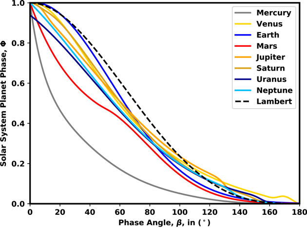
Figure 1. Melded solar system planet phase functions.
Download figure:
Standard image High-resolution imageBrown (2005) took the general planet–star separation equation and reduced it into a function of phase angle, by adding our circular orbit simplification we get

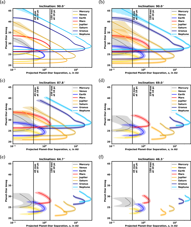
We plot the Δmag versus s curves for each solar system planet in Figure 2 at varying inclinations with HabEx angular measurement uncertainty of σWA = 0.05 mas at 10 pc and Δmag uncertainty derived from HabEx Study Team (2019) to be σΔmag = 0.145. This photometric uncertainty assumes a signal-to-noise ratio of 7 will be achieved on every planet and is achievable across the entire Δmag range of the planets. We plot the measurement uncertainty bounds by sampling Δmag and s over β and plotting the resulting 1σ bounds in Figure 2(a) and 3σ in Figures 2(b)–(f). The Δmag versus s curves in Figure 2(a) show 21 different locations where planet pairs have coincidence in the edge-on system. As the system inclination changes from edge-on to face-on in Figures 2(b)–(f), we see the number of intersections and visible range of the planets decrease. These Δmag versus s curves give us the core components required to find the (s, Δmag)-coincidence for any give planet pair.
Figure 2. Δmag vs. s plots of solar system planets for varying star system inclinations with separation lines at working angles of 45 and 150 mas at 10 pc. The 1σΔmag = 0.01% and 1σs
= 5 mas (HabEx Study Team 2019) are plotted in (a). The 3σ bounds are plotted in (b)–(f) for varying inclinations: (b) i = 90°; (c) the Earth–Saturn intersection where i ≥ 87 8; (d) the Earth–Mercury intersection where i ≥ 690; (e) the Earth–Mars intersection occurring where i ≥ 647; (f) the Earth–Venus intersection occurring at i ≥ 463. Additional Earth–Uranus and Earth–Neptune intersections occur at i = 10 and i = 17, respectively, and can be seen in (a) and (b). The phase functions for these planets are included in the Appendix. Planet radius, geometric albedo, and orbital radius are as in Table 1. Note that Saturn's Δmag calculation omits the light contribution from the rings which can quadruple the brightness (Dyudina et al. 2005).
Download figure:
Standard image High-resolution image
3. (s, Δmag)-coincidence Points
We cannot solve for (s, Δmag)-coincidence using conventional root-finding techniques because the underlying equations are nonlinear, their combination is underconstrained, and we do not know good initial guesses of the (s, Δmag)-coincidence points. This problem has three degrees of freedom: the phase angle of each planet (βs and βl for the interior and exterior planet, respectively) and the inclination of the common orbital plane. We only have the Δmag and s constraint equations making this problem underconstrained. To circumvent this issue, we formulate the problem as a constrained minimization problem and include i as a constraint on βs and βl .
In our optimization formulation, we minimize the absolute difference between the Δmag values of each planet, Δmag error. We additionally require both planets have the same planet–star separation. For each planet–star separation, there are two associated Δmag values. The larger Δmag, and therefore the dimmer side, occurs where β > 90°. The smaller Δmag, and therefore the brighter side, occurs where β < 90°. When optimizing, it is not possible for βs or βl to cross the infinite slope point of the Δmag versus s curve. We therefore formulate four separate optimization initial conditions and phase angle constraints associated with the portions of the phase curve the interior and exterior planets could have coincidence on: where the interior–exterior planets are brighter–dimmer, brighter–brighter, dimmer–dimmer, and dimmer–brighter, which we label as Q ∈ {0, 1, 2, 3}. Therefore, there are four sets of initial guesses of (βs,0,βl,0) to test the optimization process, which we differentiate with Q ∈ {0, 1, 2, 3}:
The 0.3 and 0.7 values were selected to create a midpoint value between the minimum and maximum possible β for the interior and exterior planet.
Algorithm 1. Minimum Δmag error producing phase angles
Download table as:
ASCIITypeset image
Input:
i, as
, al
, Rs
, Rl
, ps
, pl
,  ,
,  , and Q
Output:
 and
and  , the optimal planet phase angles of the small as
and large al
planet respectively
, the optimal planet phase angles of the small as
and large al
planet respectively


We run Algorithm 1 over each unique pair of solar system planets and each constraint associated with Q ∈ {0, 1, 2, 3}. Some of these optimization processes do not successfully terminate. This occurs when the inclination constraints do not allow the separation constraint to be satisfied. While other optimization formulations may successfully terminate via convergence to a minimum error solution, not all minimum error solutions are locations of (s, Δmag)-coincidence. We apply a threshold, defining planet pairs with ∣Δmags − Δmagl ∣ < 10−5 as coincident. This selection forces the omission of the Mars–Uranus intersection despite the two planets having a substantial region of overlapping uncertainty, but still includes the Earth–Saturn intersection. Table 2 contains the s and Δmag of coincidence as well as the phase angles of the interior and exterior planet. Only the Mars–Jupiter pair has two (s, Δmag)-coincidence points. There are only five instances where (s, Δmag)-coincidence occurs over a phase angle region using the Lambert phase function. They occur for Jupiter at Jupiter–Neptune, Jupiter–Uranus, Mars–Jupiter (1), and Mars–Jupiter (2) as well as Saturn–Neptune.
Table 2. Planet–Planet Coincidence Locations
| Δmag | s (au) | βs (deg) | βl (deg) | δ icrit (deg) | P1σ s | P1σ l | P2σ s | P2σ l | P3σ s | P3σ l | |
|---|---|---|---|---|---|---|---|---|---|---|---|
| Mercury–Venus | 25.41 | 0.26 | 42.18 | 158.94 | 21.06 | 7.8 | 4.7 | 14.7 | 9.6 | 20.5 | 13.9 |
| Mercury–Earth | 27.72 | 0.36 | 111.84 | 158.94 | 21.06 | 4.8 | 3.7 | 9.6 | 7.8 | 14.5 | 11.4 |
| Mercury–Mars | 26.57 | 0.38 | 81.16 | 14.54 | 14.54 | 3.3 | 2.2 | 6.7 | 4.4 | 11.5 | 6.7 |
| Mercury–Uranus | 26.13 | 0.36 | 67.06 | 1.06 | 1.06 | 3.6 | 0.0 | 7.3 | 0.0 | 11.1 | 0.0 |
| Mercury–Neptune | 27.2 | 0.38 | 99.27 | 0.73 | 0.73 | 5.8 | 0.0 | 11.5 | 0.0 | 16.1 | 0.0 |
| Venus–Earth | 23.15 | 0.72 | 92.46 | 46.27 | 46.27 | 7.9 | 5.5 | 14.8 | 11.0 | 21.7 | 15.9 |
| Venus–Saturn | 22.72 | 0.69 | 73.37 | 4.15 | 4.15 | 5.1 | 0.1 | 10.2 | 0.2 | 16.6 | 0.3 |
| Earth–Mars | 26.6 | 0.65 | 139.34 | 25.32 | 25.32 | 4.7 | 3.9 | 9.5 | 7.6 | 14.2 | 11.0 |
| Earth–Saturn | 22.8 | 0.29 | 17.06 | 1.75 | 1.75 | 2.5 | 0.5 | 4.9 | 1.0 | 7.5 | 1.4 |
| Earth–Uranus | 26.13 | 0.76 | 130.77 | 2.26 | 2.26 | 5.1 | 0.0 | 10.2 | 0.1 | 15.0 | 0.1 |
| Earth–Neptune | 27.12 | 0.53 | 148.27 | 1.0 | 1.0 | 3.6 | 0.0 | 7.2 | 0.0 | 10.8 | 0.0 |
| Mars–Jupiter (1) | 27.48 | 1.48 | 76.61 | 163.45 | 16.55 | 4.1 | 0.9 | 7.9 | 2.2 | 11.2 | 3.3 |
| Mars–Jupiter (2) | 32.98 | 0.27 | 169.67 | 176.99 | 3.01 | 0.8 | 0.3 | 1.6 | 0.5 | 2.4 | 0.7 |
| Mars–Uranus | 26.2 | 0.0 | 0.0 | 0.0 | 0.0 | 0.0 | 0.1 | 0.2 | 0.2 | 0.4 | 0.3 |
| Mars–Neptune | 27.22 | 1.38 | 65.07 | 2.64 | 2.64 | 3.5 | 0.2 | 7.5 | 0.4 | 11.0 | 0.5 |
| Jupiter–Saturn | 22.83 | 4.58 | 118.24 | 28.58 | 28.58 | 1.8 | 0.7 | 3.6 | 1.4 | 5.5 | 2.0 |
| Jupiter–Uranus | 26.1 | 2.18 | 155.24 | 6.52 | 6.52 | 0.7 | 0.3 | 1.4 | 0.6 | 2.1 | 0.9 |
| Jupiter–Neptune | 27.19 | 1.58 | 162.36 | 3.01 | 3.01 | 0.5 | 0.2 | 1.0 | 0.4 | 1.5 | 0.5 |
| Saturn–Uranus | 26.19 | 5.47 | 145.21 | 16.55 | 16.55 | 0.6 | 0.3 | 1.2 | 0.6 | 1.8 | 0.9 |
| Saturn–Neptune | 27.27 | 4.35 | 153.02 | 8.32 | 8.32 | 0.4 | 0.2 | 0.9 | 0.4 | 1.3 | 0.6 |
| Uranus–Neptune | 27.66 | 19.16 | 93.89 | 39.61 | 39.61 | 4.9 | 0.2 | 7.8 | 0.4 | 9.1 | 0.6 |
Note. The planet–star difference in magnitude, Δmag, planet–star separation s in au, phase angle of the interior planet (βs ) in deg, phase angle of the exterior planet (βl ) in deg, maximum system inclination where intersections occur (δ icrit) in deg of the planet–planet coincidence, the probability the smaller semimajor axis planet is within n σ of the intersection point (Pn σ s ) in %, and the same probability for the larger semimajor axis planet (Pn σ l ). Rounding means probabilities of 0 are less than 0.05%.
Download table as: ASCIITypeset image
With these phase angles of coincidence, we can calculate the deviations from edge-on inclinations where the solar system no longer has (s, Δmag)-coincidence for any given planet pair. We define these critical inclination deviations as (δ icrit,±). They can be found by

4. Fraction of Affected Solar Systems
We consider the Earth's Δmag versus s curve in Figure 2, which we take as representative of the highest scientific priority exoplanet type. The Earth's curve crosses those of Mercury, Neptune, Uranus, Mars, Venus, and Saturn (within the 3σ uncertainty region). Furthermore, the critical inclinations in Table 3 indicate (s, Δmag)-coincidence persists across a broad range of inclinations.
Table 3. The Percent of Solar Systems where Each Respective Planet Having Any (s, Δmag)-coincidence with Earth
| Neptune | Saturn | Uranus | Mercury | Mars | Venus | |
|---|---|---|---|---|---|---|
| % of Solar Systems | 1.7% | 3.0% | 3.8% | 36.0% | 42.7% | 72.2% |
Note. Assumes circular orbits and coplanar planet orbits.
Download table as: ASCIITypeset image
When simulating a multitude of inclined star systems, we randomly sample inclinations such that the probability density function is  following after Brown (2005), Savransky et al. (2009), and Keithly et al. (2020). Since we are assuming circular orbits, we can calculate the percentage of randomly generated solar systems where any solar system planet will have (s, Δmag)-coincidence with the Earth by integrating over the inclination probability density function,

This distribution of inclinations peaks at i = 90° (edge-on) and has minimums at i = 0° and i = 180°. We compute these probabilities and compile them in Table 3.
Table 3 shows the fraction of solar systems with (s, Δmag)-coincidence independent of instrument capabilities. We can determine which intersecting planet pairs are visible to an instrument by comparing the Δmag and s of intersection with the instrument limited Δmag ( ) and working angle limits at a star distance. For the Earth's (s, Δmag)-coincidence referenced in Table 3, an instrument with a contrast of 10−10 and inner working angle of 45 mas at 10 pc would only be able to see Earth's coincidence with Venus. As we can see from Table 2, increasing the limiting Δmag of a telescope exacerbates the potential for planet-type confusion by including more instances of (s, Δmag)-coincidence. Assuming the same instrument as in Table 3, only the Earth–Venus, Venus–Saturn, and Jupiter–Saturn coincidences are detectable. If, at some point in the future, a contrast of 10−11 with an inner working angle of 30 mas were achievable; then 15 intersections could be observable in solar system analogs.
Assuming a system produces (s, Δmag)-coincidence between two planets, we can compute the probability a planet randomly located along its orbit is within n
σ of the coincidence point. We randomly sample inclinations from  between the critical inclination limits and randomly distribute these planets uniformly in time along their orbit. s and Δmag of each randomly sampled planet can be computed and we can find the fraction of these planets within the n
σ uncertainty region of the (s, Δmag)-coincidence point. This fraction is the fraction of an orbit the planet spends within this uncertainty region and is converted into the percentages in Table 2. In all cases, the probability of the larger semimajor axis planet being within the uncertainty bounds is less than the probability of the smaller semimajor axis planet being within the measurement uncertainty bounds (Pn
σ
l
< Pn
σ
s
). The maximum probability of coincidence is between Venus–Earth followed by Mercury–Venus, Mercury–Earth, and Earth–Mars. If a planet from a solar-system-like star system at the (s, Δmag)-coincidence of Earth with either Uranus or Neptune is detected, it is ∼150× more likely that the planet is an Earth than a Uranus or Neptune. In general, the probabilities of either planet being within the instrument uncertainty bounds are within an order of magnitude of one another. Only the instances of Mercury–Uranus, Mercury–Neptune, Venus–Saturn, Earth–Uranus, and Earth–Neptune have occurrence disparities greater than an order of magnitude.
between the critical inclination limits and randomly distribute these planets uniformly in time along their orbit. s and Δmag of each randomly sampled planet can be computed and we can find the fraction of these planets within the n
σ uncertainty region of the (s, Δmag)-coincidence point. This fraction is the fraction of an orbit the planet spends within this uncertainty region and is converted into the percentages in Table 2. In all cases, the probability of the larger semimajor axis planet being within the uncertainty bounds is less than the probability of the smaller semimajor axis planet being within the measurement uncertainty bounds (Pn
σ
l
< Pn
σ
s
). The maximum probability of coincidence is between Venus–Earth followed by Mercury–Venus, Mercury–Earth, and Earth–Mars. If a planet from a solar-system-like star system at the (s, Δmag)-coincidence of Earth with either Uranus or Neptune is detected, it is ∼150× more likely that the planet is an Earth than a Uranus or Neptune. In general, the probabilities of either planet being within the instrument uncertainty bounds are within an order of magnitude of one another. Only the instances of Mercury–Uranus, Mercury–Neptune, Venus–Saturn, Earth–Uranus, and Earth–Neptune have occurrence disparities greater than an order of magnitude.
5. Conclusion
Future exoplanet direct-imaging missions must make multiple observations to differentiate between Earth-like exoplanets and the myriad of other planets in the population. We took phase functions derived from a variety of deep space missions to create melded phase functions of solar system planets. We showed that up to 21 cases of (s, Δmag)-coincidence between planet pairs exist in the solar system. We additionally showed how an Earth can have the same (s, Δmag)-coincidence with up to six other solar system planets. We found the inclination range where each solar system planet could still have coincidence with another planet. We found 36%–69% of inner solar system planets and 1%–4% of outer solar system planets share (s, Δmag)-coincidence with Earth. While the Nancy Grace Roman Space Telescope would only be capable of seeing coincidences between Earth and Venus, further improvement in instrument contrast and inner working angles will exacerbate the planet confusion problem.
This work was funded by the Science Investigation Team of the Nancy Grace Roman Space Telescope under NASA grant NNX15AB40G.
Appendix: Solar System Planet Phase Functions
Here, we combine the phase functions extracted from the model fit visual magnitude functions (Vmag) of each solar system planet in Mallama & Hilton (2018) using the parameterized hyperbolic tangent functions to meld parametric phase functions into a continuous phase function. In β ranges where a phase curve model for the planet is unavailable, we "fill in the gaps" by substituting in the Lambert phase function (Equation (4) from Brown 2005).
In general, we have knowledge of the phase function over most of the β range for Earth and planets interior to Earth. The phase date we have for planets exterior to Earth are limited to the phase angles observable by Earth and the ranges imaged via various flybys. The regions generally requiring melding with the Lambert phase function to span the β range are in excess of 130° and are where the planet is dimmest and least detectable.
Mercury's phase function is given by
It spans the entire β range and does not require melding.
Venus's phase function is separated over two regions. The first,
is defined from 0° ≤ β ≤ 1637. The second,
is defined over the region 1637 ≤ β ≤ 179°. The parametric phase functions have minor discontinuities that we account for by adding a constant to and scaling the second parametric phase function into
Finally, we meld Φint,♀,1(β) and Φint,♀,3(β) together using the hyperbolic tangents to arrive at Venus's melded phase function
The phase function for Earth spans the range of β and is

Mars's phase function is separated over two regions. The first,

is valid from 0° ≤ β ≤ 50°. The second,

is valid over 50° < β ≤ 180°. We need to normalize Φint,♂,2(β) to account for discontinuities between the two phase functions and arrive at the corrected second phase function of

Combining these two phase functions, we get Mars's melded phase function
In the original formulation from Mallama & Hilton (2018), both parametric Vmag functions of Mars vary depending upon the rotational and orbital longitude of the planet. We assume the average of these correction terms, which are both 0.
The phase function for Jupiter is defined over two separate regions. The first is

The second is
We offset Φint,♃,2(β) accounting for the the last valid value of Φint,♃,1(β) to arrive at the modified second phase function of
We then combine the phase functions for Jupiter to get
The phase function for Saturn is complicated by measurements of the planet obfuscated and augmented by the rings that have a unique phase function from the planet. The phase function of Saturn without the rings is defined over two separate regions. The first,

is based on Earth observations valid from 0° ≤ β ≤ 65. The second,
is defined over the range 6° ≤ β ≤ 150°. By properly adjusting the discontinuity between the first and second phase functions, we arrive at
We combine the phase functions for Saturn to get
Uranus has a unique phase function due to the inclination of the pole's rotational axis, but only has one phase function. We assume a subsolar latitude of − 82°, which makes Uranus as bright as possible by adding a 0.0689 correction to the phase function (the minimum correction occurs at 82° and adds −0.0689). The phase function for Uranus is

valid over the range 0° ≤ β ≤ 154°. The combined phase function model for Uranus is
Neptune has two phase functions, one based on Earth measurements that cover such a small range of phase angles that we ignore it and use the phase curve from Voyager 2 radiometer measurements. Neptune's one phase function is

and is valid over the range 0° ≤ β ≤ 13314. The combined phase function for Neptune is therefore