


Abstract
We present a new method to semianalytically calculate the radiation efficiency of electromagnetic waves emitted at specific frequencies by electrostatic wave turbulence in solar wind and coronal plasmas with random density fluctuations. This method is applied to the case of electromagnetic emission radiated at the fundamental plasma frequency ωp by beam-driven Langmuir wave turbulence during Type III solar bursts. It is supposed that the main radiation mechanism is the linear conversion of electrostatic to electromagnetic waves on the background plasma density fluctuations, at constant frequency. The radiation efficiency (emissivity) of such a process is larger than that obtained in the framework of models where the low frequency density fluctuations and the corresponding ion sound waves are not external but produced by the electrostatic wave turbulence itself through nonlinear wave–wave interactions. Results show that the radiation efficiency of Langmuir wave turbulence into electromagnetic emissions at ωp is nearly constant asymptotically, with the electromagnetic energy density growing linearly with time, and is proportional to the average level of density fluctuations. Comparisons with another analytical method developed by the authors and with space observations are satisfactory.
Export citation and abstract BibTeX RIS
1. Introduction
Electromagnetic radiation associated with Type III solar radio bursts has been observed for a long time both by ground-based radio telescopes and on board spacecraft (e.g., Bougeret et al. 1970; Lin 1974; Fitzenreiter et al. 1976; Gurnett & Anderson 1977; Steinberg et al. 1984; Suzuki & Dulk 1985; Lin et al. 1986; Reiner et al. 1992; Benz et al. 2007). It is believed that these radio bursts' emissions at the electron plasma frequency ωp and its harmonic 2ωp are the result of a chain of events in which electron flows accelerated during solar flares are generated and emit Langmuir wave turbulence via beam instability during their propagation in the coronal and solar wind plasmas up to distances of 1 au from the Sun and beyond (Zheleznyakov & Zaitsev 1970; Grognard 1975; Goldman 1983; Mel'nik et al. 1999). In turn, the beam-driven Langmuir waves release part of their energy to electromagnetic radiation. Various mechanisms have been proposed to explain such energy transfer from electrostatic waves to electromagnetic ones. Among the most important, it is worth mentioning the processes of nonlinear wave interactions (Ginzburg & Zheleznyakov 1958; Melrose 1980), including the decay of Langmuir waves  into ion sound waves
  and transverse electromagnetic waves
  of frequency ωp (
 ), or the fusion of
  and
and  waves along the channel
  . Moreover, it is believed that the electromagnetic emissions
  at 2ωp result from the coalescence
  of two Langmuir waves
  and
and  , which are driven by the beam and produced by the electrostatic decay
  respectively. Typically, these processes were considered in the framework of the weak turbulence theory. However, in some works, the electromagnetic radiation at ωp was studied using the strong turbulence theory (Papadopoulos et al. 1974), assuming that Langmuir wave fields captured in collapsing cavitons and Langmuir solitons can emit such waves (Galeev & Krasnosel'skikh 1976; Goldman et al. 1980); numerical simulations performed in the strong turbulence regime confirmed the main features of these emissions (Akimoto et al. 1988).
Using realistic Langmuir and ion sound waves' spectra, the theory of weak turbulence allowed for analytical calculations of the rates of electromagnetic emissions generated at ωp by the wave decay  (Edney & Robinson 1999). In another work (Willes et al. 1996), a similar method was used to analytically estimate the radiation rate corresponding to the coalescence process
  . Moreover, numerical simulations conducted in the framework of weak turbulence (e.g., Kasaba et al. 2001; Li et al. 2009; Li & Cairns 2013; Ratcliffe et al. 2014) reproduced part of the characteristic features of the dynamics of the observed emission spectra.
Alternative approaches were based on linear conversion mechanisms (Field 1956) of Langmuir or z-mode waves to electromagnetic radiation in plasmas with density gradients. Various aspects of such processes were considered by several authors (Melrose 1980; Cairns & Willes 2005; Yu & Kim 2013; Schleyer et al. 2014); in particular, it was shown that such mechanisms may explain the radio emissions by Type III solar bursts (Thejappa et al. 1993). The effectiveness of linear conversion mechanisms was also investigated using numerical methods (Cairns & Willes 2005; Kim et al. 2008).
On the other hand, it was found that the solar wind plasma is characterized by a large variety of density fluctuations (Celnikier et al. 1983; Kellogg & Horbury 2005). For example, satellites' measurements revealed that density fluctuations δn around several percent of the average background plasma density n0 exist in the solar wind, with length scales around a few hundreds of kilometers (Mugundhan et al. 2017; Chen et al. 2018; Krupar et al. 2018). These fluctuations, even when weak, affect the development of the electron beam instability and of the intensity and the spectra of the emerging Langmuir wave turbulence (Volokitin et al. 2013; Krafft et al. 2013, 2014, 2015, 2019; Krafft & Volokitin 2014, 2016b; Voshchepynets et al. 2017). In particular, it was shown (Krafft et al. 2015; Krafft & Volokitin 2016a) that the electrostatic decay  is less efficient and more localized in space and time in a plasma with density fluctuations than in a uniform plasma. Thus, one can reasonably assume that under such conditions other nonlinear wave processes such as the coalescence
  or the decay
  can be weakened in a plasma with inhomogeneities.
Moreover one should note that, as the emissivity of electrostatic wave turbulence into electromagnetic radiation is proportional to the spectral electric field energy and density fluctuation intensity  , the linear mechanism of wave conversion on external density inhomogeneities is more efficient to generate electromagnetic radiation than the nonlinear wave–wave interaction processes proposed in the frame of the weak turbulence theory. In the latter case the density fluctuations are much weaker (at least by one order of magnitude) because they are induced and depend on the wave turbulence itself; then the corresponding radiation efficiency has a nonlinear dependence on the Langmuir spectral energy, explaining why the wave conversion mechanism leads to larger emissivities (note that the turbulence parameters considered are weak). Moreover, external density fluctuations cannot be neglected in solar wind plasmas, so that a realistic theoretical description cannot avoid taking into account interactions of waves with such density structures. Finally, in the framework of the weak turbulence model, not all small amplitude ion sound waves forming the spectrum
  can satisfy the resonance conditions required to produce electromagnetic waves through resonant wave–wave nonlinear interactions.
In view of this, the attention to the mechanism of linear transformation of waves on density gradients has increased. Moreover, in solar wind and coronal plasmas, the presence of fluctuating density irregularities leads to the multiple appearance of boundaries between plasma regions of different densities where wave transformations such as refraction, reflection, tunneling, and conversion phenomena occur. Then, using an original approach and realistic wave and density fluctuations' spectra, some authors (Krasnoselskikh et al. 2019) calculated the conversion efficiency of Langmuir waves and obtained estimates in good agreement with the observations. Recently, a new method of determination of the radiation efficiency of electrostatic wave turbulence was proposed (Volokitin & Krafft 2018), which is based on the direct calculation of the electromagnetic fields emitted at large distances by a plasma source with high-frequency electric currents oscillating at the plasma frequency, determined using a model of Langmuir wave turbulence in a plasma with external background density fluctuations. The semianalytical calculation of the radiation efficiency showed a satisfactory agreement with space observations.
In this paper we present another new semianalytical method of calculation of the efficiency of electromagnetic wave radiation at the frequency ωp from a plasma with Langmuir wave turbulence and random density fluctuations. As in a previous work (Volokitin & Krafft 2018), it is assumed that the main mechanism responsible for the generation of electromagnetic waves is the linear conversion of electrostatic waves on the external density fluctuations. Unlike the theory of weak turbulence for a homogeneous plasma, the assumption of weak correlations between the waves is not necessary and, since the electromagnetic emissions do not arise from three-waves' resonant interactions but result from the transformations of Langmuir waves on the density fluctuations, we do not need to take into account exact resonance conditions between the waves.
2. Electromagnetic Wave Radiation by a Turbulent Plasma with Random Density Fluctuations
In a previous paper (Volokitin & Krafft 2018) we calculated the radiation efficiency at far distances of a plasma source with external random density fluctuations and Langmuir wave turbulence emitting electromagnetic waves. The two-dimensional high-frequency current oscillating at the plasma frequency ωp within the source was calculated owing to the Zakharov equations. Then, by solving an inhomogeneous Klein–Gordon equation involving this current and derived from the Maxwell equations with the help of Green functions, and by using a modified theory of retarded potentials, the electromagnetic energy density emitted at ωp and the corresponding radiation efficiency were determined as a function of the average level of density fluctuations  , the ratio c/vT (vT is the plasma thermal velocity), and the position of the observer with respect to the source. This method provided radiation efficiencies that were in good agreement with satellite observations of Type III radio bursts' emissions.
Hereafter we present a new and more effective semianalytical method aimed at calculating the radiation efficiency of electrostatic wave turbulence. Let us consider a solar wind plasma source involving Langmuir turbulence and external density fluctuations of average level ΔN ≃ 0.01–0.06, characterized by wavelengths of several hundreds of electron Debye lengths λD. These waves scatter on the random density inhomogeneities and can be linearly converted into electromagnetic waves at a constant frequency close to ωp.
Indeed, due to the presence of external density fluctuations, the dominant process responsible for the radiation of electromagnetic waves  at the frequency ωp is the linear conversion of Langmuir waves
  on the inhomogeneities (Denisov 1957; Stix 1965; Cairns & Willes 2005; Kim et al. 2008; Schleyer et al. 2014), and not the nonlinear wave–wave resonant interactions
  involving ion sound waves
  corresponding to induced and weak ion density perturbations. The transformation of Langmuir waves on the external density fluctuations produce an electronic current of the first order whose rotational part is responsible for the radiation of electromagnetic waves as a result of refraction phenomena occurring when the electrostatic waves interact with the density fluctuations. The dynamics of this current can be calculated by solving the Zakharov equations on a 2D map representing the inhomogeneous solar wind plasma. All phenomena of reflection, refraction, and tunneling of waves are taken into account in the simulations. The initial levels of the Langmuir waves' and fluctuations' spectra are chosen according to realistic conditions; their profiles take into account possible anisotropies and the expected wavevector ranges, inferred from results obtained during one-dimensional studies performed by the authors (Volokitin et al. 2013; Krafft et al. 2013, 2014, 2015, 2019; Krafft & Volokitin 2014, 2016b; Voshchepynets et al. 2017). The rotational part of the calculated electronic current generates the induced electromagnetic wave fields as a result of the conversion, at constant frequency, of the electrostatic wave turbulence. The produced waves are then leaving the volume with density fluctuations where they are generated and propagate freely and without loss through the surrounding homogeneous plasma. The model allows us to calculate the emissivity of this first-order wave conversion process owing to numerical simulations confirmed by analytical estimates, as shown below.
The equation describing the electromagnetic waves' dynamics can be obtained from the Maxwell equations
where δ is the wave's magnetic field perturbation. The high-frequency electronic current δ
 produced by the scattering of Langmuir waves on the external density fluctuations is

where δn is the slowly varying electron density perturbation and  is the fast velocity oscillation (at ωp) of the electron population; e < 0 and me are the electron charge and mass. The Langmuir wave's potential perturbation is given by
  , where
  is the slowly varying potential envelope. Note that δ
 is a first-order term as the density fluctuations δn are given at the initial state and not induced during the system's dynamics. Then we get
where n0 is the background plasma density and  ωs ≪ ωp is the ion acoustic frequency. Assuming that
  , where
  ≃ ωp is the frequency of the electromagnetic wave and
  is the slowly varying envelope of its magnetic field, we find that

where we used that  . Equation (4) can be written in the wavevector space as
with 
 is the wavevector and
  the position. Note that the right-hand side term of Equation (5), proportional to the current density in the plasma source, is calculated by solving at each time moment the 2D Zakharov equations (Volokitin & Krafft 2018). The homogeneous equation corresponding to Equation (5) can be solved exactly as follows
A particular solution of Equation (5) is obtained in the form
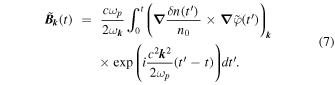
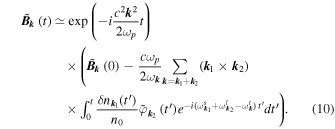
Combining the solutions (6)–(7), we obtain the Fourier component of the magnetic field envelope at time t

For sufficiently large  above a threshold
  , the function
  oscillates quickly. Therefore, the main contribution to the integral in Equation (8) is due to the long-wavelength part (with
  ) of the term
  . As the simulations performed to calculate δn and
  from the 2D Zakharov equations show, this term slowly changes with time, so that it can be extracted from the integral. On the other hand, we note that, for
  , the oscillation rates
  of the plasmon phases
  turn out to be important and comparable with
  therefore, we distinguish the phases explicitly from the amplitudes by setting below
  . Moreover, one can write that

where  and
and  are the wavevectors corresponding to the Fourier components of the density perturbations and the Langmuir wave potential, respectively. Then we get from Equation (8) that
We took into account the dispersion relation of the transverse electromagnetic wave in a homogeneous plasma, i.e.,  , so that
  , where the Langmuir wave frequency is
  with
with  ;
;  is the ion sound frequency; as mentioned above, the main contribution to the electromagnetic emission at
  in the summation
  comes from the domain of small wavevectors satisfying
  . Note that since we are not considering here parametric resonant interactions between waves, but their transformations on density fluctuations, we do not need to fulfill exactly the three-waves' resonance condition
  . Let us mention that Equation (10) can be compared with the expressions providing the growth rate of the energy density of an electromagnetic wave
  produced by the fusion
  of a Langmuir wave
  and an ion sound wave
  , in the frame of the weak turbulence theory (Melrose 1987; Edney & Robinson 1999).
By raising Equation (8) squared and neglecting the terms proportional to the initial wave magnetic field  , whose amplitude is around the noise level (note that these terms vanish also after the average performed below), we get
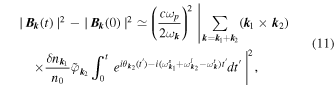
where we took into account that the potential's amplitude varies much more slowly than its phase. The wavevectors of the electromagnetic waves satisfying  , the spatial synchronism condition
  can be written as
  , so that Equation (11) can be presented in the following form
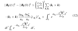
where the superscript "*" denotes the complex conjugate. Assuming the absence of correlations between the density fluctuations, let us average on the phases
and simplify further Equation (12)
Let us now show that asymptotically the following relation is fulfilled

where the dimensionless function  is estimated below. If it is possible to neglect the variations of the plasmons' phases
  in Equation (14), i.e., if
  for sufficiently large
  , then
  does not depend on
  and is asymptotically proportional to the Dirac function
  Indeed, summing Equation (13) on
  , its right-hand side term becomes of the form
where  is a continuous function. It follows that, asymptotically, the electromagnetic wave energy density
  (13) increases linearly with time within a narrow region of wavevectors near
  ≃ 0, whereas the size of this region, where electromagnetic waves are generated, decreases with time. This compression stops when the size reaches a value for which the phase
  begins to exceed
  . Therefore we consider below the case of small
  for which
  , i.e., when the phases
  turn out to be decisive for the calculation of
  .
.
The time dependence of the plasmons' phases is random by nature and determined by their distribution in the inhomogeneous plasma. However, averaging over the random phase variations allows us to state certain conclusions if we assume that  and that the rates
  are randomly distributed. Then we can write that
Assuming that the rates  are uniformly distributed, we get

It follows that the electromagnetic wave energy density  depends linearly on the time t. Indeed, for large t, the phase interval over which the integration in Equation (17) is performed is large, so that the integral
  depends very weakly on the boundaries of the variation range
  . Finally we can conclude that, in the general case,
  is a function that decreases sharply for
  and mainly depends on
  for
for  . Unfortunately, at this stage, it is only possible to estimate the order of magnitude of
  and
and  . Since both quantities are due to the presence of density fluctuations, the dispersion of electromagnetic waves allows us to write that
  and
and 
In conclusion, this analysis allows us to state that, at asymptotic times, the energy density  of the electromagnetic waves generated by a stationary Langmuir wave turbulence via linear transformation mechanisms on density inhomogeneities increases linearly with time. In actual conditions, when the electromagnetic waves have the ability to freely leave the turbulent source, we can speak of a quasi-constant rate of conversion of Langmuir waves' energy into an electromagnetic one. So, we assume that all the energy transformed in a given volume leaves it and propagates without loss outside the source through the external uniform plasma. Then the electromagnetic power radiated is determined by
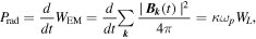
where  is the electromagnetic wave energy density and
  is the Langmuir wave energy density in the volume Vrad of the emitting source. The dimensionless quantity κ is the ratio of the energy of electromagnetic waves radiated from a given volume of plasma during the period
  to the energy of Langmuir waves in the same volume. The following expression can be obtained from the theoretical analysis presented above
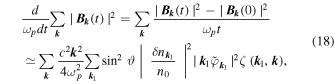
where ϑ is the angle between the plasmon wavevector  and the small electromagnetic wavevector
  . In the case of quasi-isotropic wave spectra we can write that
  so that

where  . As the term
  in Equation (19) is not sufficiently defined at this stage, we have to turn to numerical simulations. Nevertheless, using the estimates
  ,
,  and
and  , and omitting possible numerical factors, we can write that
  Thus, one can expect a weak dependence of S on ΔN, or even no dependence, as confirmed by the numerical simulations. In this case, the scaling
  follows from Equation (19) with
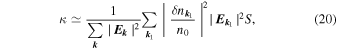
where S can be interpreted as a fraction of phase volume in the  -space corresponding to the fraction of plasmons with wavevectors
  transformed on density fluctuations into electromagnetic waves of close wavevectors. Note that, in Equation (20), only the factor S contains a possible dependence on the speed of light c; from a formal point of view, one can expect that
  if
if  . Indeed, the radiation intensity of a localized current source decreases with increasing ratio of the emitted wavelength (proportional to c) to the size of the source, and tends to zero when
  . This remains true in the case of linear transformations of electrostatic waves into electromagnetic ones when they scatter on inhomogeneities of finite size.
Let us now compare the analytical results obtained above with those provided by the numerical simulations performed on the basis of a 2D modeling of Langmuir wave turbulence in a plasma with density inhomogeneities (see the description in Volokitin & Krafft 2018), which allows us to determine the distribution of the high-frequency electronic currents in a given plasma source region. Next, solving Equation (5) numerically or, equivalently, calculating the wave magnetic field using Equation (8), we can find the time evolution of the electromagnetic waves' amplitudes according to the numerical scheme described in the Appendix where, in particular, the necessary restriction on the discretization time step is indicated. It was shown that numerical results are stable under this condition.
The main conclusions provided by the simulations are consistent with those derived analytically above, namely, the linear growth with time, at the asymptotic stage, of the electromagnetic energy density emitted by the turbulent plasma volume. Therefore, it is possible to determine, using the simulation results, the rate of the ratio of the electromagnetic wave energy to the energy of electrostatic Langmuir waves, that is, the radiation efficiency defined according to
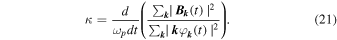
We used the same notation κ for the value obtained theoretically in Equation (20) and for the definition of the radiation efficiency presented in Equation (21), as in both cases the physical meaning is the same.
The variations of κ as a function of the two characteristic parameters c/vT and ΔN have been studied (vT is the plasma thermal velocity). They were obtained by using Equation (21) with fields computed by the numerical simulations. Note that all variables below are normalized according to  ,
,  , and
, and  , where Te is the electron temperature of the background plasma. All analyses illustrated hereafter by figures were performed within time intervals where wave spectra were quasi-stationary.
Figure 1 shows the electromagnetic wave spectra at asymptotic times, for three values of the ratio c/vT and a fixed average level of density fluctuations ΔN. One can see that, as it should be, the size of the  -space where electromagnetic waves are generated does not depend on the time step Δt (compare the upper and the bottom panels) and is proportional to
  , so that its area scales as
  . This result is in accordance with the scaling laws presented below in Figure 3. Note also that, at the asymptotic stage, the size of the
  -space region where the electromagnetic waves' amplitudes grow does not change with time (not shown here), which confirms the conclusions obtained above when analyzing analytically
  (Equations (14)–(17)).

Figure 1. Electromagnetic wave spectra at asymptotic times (around t ≃ 9800): isocontours of the square spectral wave magnetic field  , for c/vT = 50, 70, and 100; ΔN = 0.027; kx and ky are the normalized wavevectors' components along and across the ambient magnetic field direction, respectively. The time steps used for the fields' calculations (see the Appendix) are Δt = 8 (upper panels) and Δt = 2 (bottom panels).
Download figure:
Standard image High-resolution imageFigure 2 shows the growth with time of the electromagnetic wave energy density  calculated at the asymptotic stage by the numerical simulations; the corresponding linear interpolations describe the time dependence predicted by the analytical calculations well (Equations (14)–(17)). The values of the radiation efficiency κ are proportional to the time derivatives of
  (21), i.e., to the slopes of the interpolation lines. Note that, due to the statistical oscillations which are natural to the processes considered, the time variations of the derivatives (not shown here) are noticeable compared to the linear approximations. Therefore, in order to avoid such numerical uncertainties during the calculation of κ, averaging on time was carried out, corresponding to the substitution in Equation (21) of the time derivatives by the slopes of the linear approximations.
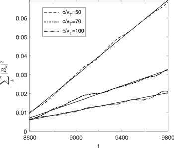
Figure 2. Growth with time, at the asymptotic stage, of the electromagnetic wave energy density  calculated by the numerical simulations (dashed and dotted lines) superposed to their linear interpolations (solid lines). Three values of c/vT are considered : 50, 70, and 100; ΔN = 0.027. All variables are normalized.
Download figure:
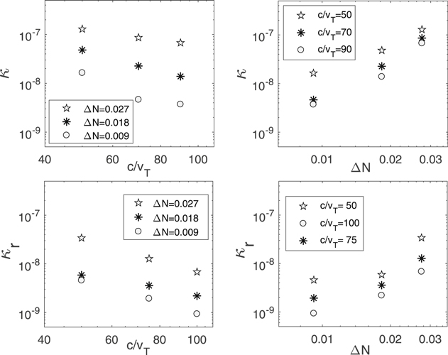
Standard image High-resolution imageThe upper panels of Figure 3 show the results of such calculations and present the dependence of the radiation efficiency κ as a function of the ratio c/vT and the level of density fluctuations ΔN, respectively. A clear dependence of κ on these parameters can be observed, even if its calculated values are more or less scattered. The radiation efficiency is shown to vary linearly with ΔN, as expected from the above analytical developments; moreover, the scaling law  obtained is in good agreement with the results provided by Figure 1 and with the above remarks concerning the behavior of S (20) with increasing c.
Figure 3. (Upper panels) Variations of the radiation efficiency κ calculated using the numerical simulations and Equation (21), as a function of the velocity ratio c/vT (for three values of ΔN = 0.009, 0.018, and 0.027, left) and the average level of density fluctuations ΔN (for three values of c/vT = 50, 70, and 90, right). The axes' scales are logarithmic. (Bottom panels) Variations of the radiation efficiency κr calculated using the numerical simulations and a method based on the theory of the retarded potentials (Volokitin & Krafft 2018), as a function of the velocity ratio c/vT (for three values of ΔN = 0.009, 0.018, and 0.027, left) and the average level of density fluctuations ΔN (for three values of c/vT = 50, 75, and 100, right). The axes' scales are logarithmic.
Download figure:
Standard image High-resolution image
These results can be compared with those obtained using the numerical simulations and another analytical method presented earlier by the authors (Volokitin & Krafft 2018), which is based on the theory of the retarded potentials. The corresponding radiation efficiency κr is shown in the bottom panels of Figure 3, as a function of c/vT and ΔN. One can see that, despite some numerical uncertainties inherent to both approaches (compare upper and bottom panels), the values of the radiation efficiencies κ and κr provided by the two semianalytical methods are in reasonable agreement. Moreover it is worth noting that the scaling laws κ ∝ ΔN and  are obtained using both approaches.
3. Conclusion
The electromagnetic radiation at the plasma frequency ωp generated by a plasma source with electrostatic wave turbulence and density fluctuations is studied theoretically and numerically. It is assumed that the main mechanism of radiation of the electromagnetic emissions is the linear transformation of Langmuir waves on the density inhomogeneities. This process is likely the most effective if the average level of density fluctuations ΔN is of the order of 1% of the background plasma density or higher, what is the case for the solar wind and coronal plasma regions where Type III solar radio bursts manifest.
We present a new method to calculate analytically the radiation efficiency of electromagnetic waves emitted at some specific frequencies by electrostatic wave turbulence in a plasma with random density fluctuations. This method, which complements another one proposed recently by the authors (Volokitin & Krafft 2018) is more convenient to use and more robust. Moreover it is shown that, despite significant differences between both approaches, the two methods lead to close values of the radiation efficiencies and provide similar scaling laws as a function of the average level of density fluctuations ΔN and the velocity ratio c/vT.
More precisely, a simple analytical expression is obtained (Equation (20)) that allows us to determine the efficiency of the electromagnetic radiation from a turbulent and inhomogeneous plasma, if the density fluctuations' and the Langmuir waves' spectra are available. In particular, it shows that the radiation efficiency depends mainly on the integral characteristics of the spectra, is weakly sensitive to detail features and is proportional to the average level of density fluctuations ΔN.
When deriving Equation (20), a number of assumptions were made that appear to be sufficiently substantiated. Nevertheless, our theoretical results were verified using numerical simulations based on a 2D modeling of Langmuir wave turbulence in a plasma with quasi-random density inhomogeneities, that confirmed our assumptions.
This work was granted access to the HPC resources of IDRIS under the allocation 2013-i2013057017 made by GENCI. This work has been done within the LABEX Plas@par project, and received financial state aid managed by the Agence Nationale de la Recherche, as part of the programme "Investissements d'avenir" under the reference ANR-11-IDEX-0004-02. This work was supported by the Programme National PNST of CNRS/INSU cofunded by CNES and CEA.
Appendix
Let us present the numerical scheme used to calculate the wave radiation intensity emitted at time t from the 2D turbulent inhomogeneous plasma source. Starting from Equation (8) that provides the magnetic field's Fourier component  , one can obtain after one time step Δt ≪ t that
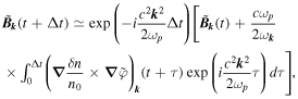
where we defined  Then, expressing the term proportional to the electronic current as follows
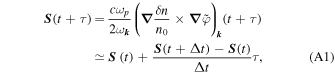
we get
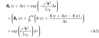
The calculation of the integrals in Equation (A2) leads to the rather simple expression
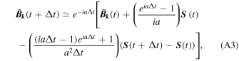
where  Note that in our case, because the electromagnetic emissions come from a very small region of the
  -space, we do not need to take into account the correlations between the density fluctuations δn/n0 and the potential's envelope
  , contrary to what is done in the frame of the weak turbulence theory. A similar formula can be obtained using Equation (5) and finite-difference methods
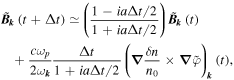
which is valid if  and if
  varies negligibly during the small time interval Δt. Then, for
  we get the simple approximate formula
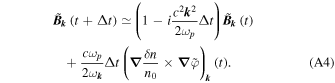
Note that  in the above study.
Using Equations (A3) or (A4) and knowing the values of  (t) (A1) at any time owing to the 2D simulations based on the Zakharov equations (see Volokitin & Krafft 2018 for more details), we can calculate numerically
  as well as the electromagnetic wave energy density WEM and the radiation efficiency κ.