


Abstract
Drifts due to the curvature and gradients in the heliospheric magnetic field, as well as along the heliospheric current sheet, have long been known to play a significant role in the transport of galactic cosmic rays. Recently, there has been greater interest in the role these drifts play in the transport of solar energetic particles. This study proposes an approach to modeling particle drift velocities in particle transport codes that, while being relatively simple to implement and computationally inexpensive, also models drift effects accurately across a broader range of energies than previous approaches.
Export citation and abstract BibTeX RIS
1. Introduction
Theoretical and numerical studies, combined with observations both ground-based and by spacecraft, have long established that drift effects play a key role in the modulation of galactic cosmic rays (GCRs; e.g., Forman et al. 1974; Jokipii et al. 1977; Jokipii & Levy 1977; Jokipii & Thomas 1981; Kota & Jokipii 1983; Burger et al. 1985; Burger 1990; Heber et al. 1996; Lockwood & Webber 2005, to mention but a few). Recently, a growing number of publications have also begun taking into account drift effects in the transport of solar energetic particles (e.g., Dalla et al. 2013, 2017; Marsh et al. 2013; Battarbee et al. 2017, 2018), with some observational evidence indicating the importance of solar energetic particle drift along the heliospheric current sheet (HCS; Augusto et al. 2019).
Several techniques have been employed in the past to incorporate current sheet drift effects into cosmic-ray (CR) modulation codes, most notably that of Burger et al. (1985), which involves numerically ascertaining whether a particle is within two Larmor radii of the current sheet, and if so calculating its drift velocity from an approximate expression; and the approach proposed by Burger (2012), which calculates drift velocities directly, given an expression for the HCS angle θns and an assumed heliospheric magnetic field (HMF) model. Both these approaches are well-suited to the stochastic differential equation approach to solving the Parker (1965) CR transport equation, which requires explicit inputs for the CR drift velocity components (see, e.g., Strauss & Effenberger 2017), and have been successfully implemented in several CR transport studies by, e.g., Strauss et al. (2011), Engelbrecht & Burger (2013), and Moloto et al. (2018). The Burger (2012) approach has the benefits of being relatively straightforward to implement, being computationally inexpensive, and of providing explicit results. The aim of this study is to propose a refinement thereof derived so as to take into account particle transport conditions in the very inner heliosphere, more relevant to the study of solar energetic particles, but still applicable to the study of GCRs.
For a nearly isotropic particle distribution, the drift velocity is given by (see, e.g., Jokipii et al. 1977)

where κA denotes the drift coefficient, and eB a unit vector along the background HMF, assumed in what follows to be a Parker (1958) field. Equation (1) by definition remains divergence free. To model the change in magnetic field direction across the HCS at colatitude θns, Burger (2012) employs a hyperbolic tangent function, and makes the substitution

where k is a numerical parameter that adjusts the steepness of the transition, and  is a geometrical factor added post facto to ensure that drift velocities along the current sheet remain smaller than the particle velocity v. Figure 1 illustrates the Burger (2012) transition function, assuming a flat (θns = π/2) current sheet, for various values of k. Larger values of k lead to a transition more closely resembling the Heaviside Step function. As a charged particle is expected to experience drift effects due to the HCS if it finds itself within two Larmor radii (RL) above or below this structure (see, e.g., Burger et al. 1985), Burger (2012) links k to the extent of the "effectiveness" of the HCS, proposing for instance that k = 20.12 for particles with rigidities less than 3.5 GV, and
  otherwise, with P the particle rigidity. This was to ensure that grid resolution would be sufficient to resolve this region around the HCS in the modulation code employed in that study to solve the Parker (1965) transport equation. It is, however, not straightforward to calculate a value of k that would ensure that the effect of the HCS on drift velocities would be appropriately taken into account for charged particles throughout the heliosphere, given variations in RL.
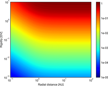
Figure 1. Burger (2012) θ-averaged current sheet drift speed for a flat HCS, normalized to the theoretical value of v/6, as function of proton rigidity and heliocentric radial distance in the ecliptic plane.
Download figure:
Standard image High-resolution imageThe drift velocity expression proposed by Burger (2012) is given by
where the first and second terms describe the velocities due to gradient/curvature drifts and drifts along the current sheet, respectively. The third term is an artifact due to the inclusion of the  term in Equation (2), and it is argued by Burger (2012) that this term does not significantly contribute to the drift flux of particles in a realistic model heliosphere. The comparative study by Kopp et al. (2017), however, finds that this third term does indeed affect their computed CR intensities, but does not show this result. To test this result, we compare it with the θ and ϕ averaged drift speed calculated by Burger (1987), who find, for a perfectly flat HCS and a uniform HMF with a change of sign across said current sheet modeled using a Heaviside Step function and computing the average over a θ interval of
  , that this speed is equal to v/6 (Burger et al. 1987). Doing the same for Equation (3), and neglecting the third term, leads to (Moloto 2015)

Figure 1 shows how Equation (4), normalized to v/6, would vary in the ecliptic plane as a function of heliocentric radial distance and proton rigidity. For rigidities greater than ∼1 GV, and radial distances greater than ∼1 au, the Burger (2012) approach almost exactly reproduces the theoretical result, implying that this approach is very suitable to modeling the drift velocities of GCRs. At lower rigidities and smaller radial distances more relevant to the transport of solar energetic particles, the agreement with theory becomes considerably worse, suggesting that this is not the ideal approach to model the effects of drift for these particles.
In what is to follow, a new approach to modeling charged particle drift velocities in the heliosphere is proposed. This approach, based on the methodology of Burger (2012), involves the use of a new transition function, which will eliminate the uncertainty implicit to the choice of k in the Burger (2012) approach as well as eliminating the third term in Equation (3). Furthermore, it will be demonstrated that this approach will be able to model current sheet drift effects for solar energetic particles to a greater degree of accuracy than the approach of Burger (2012), as well as modeling these effects to a reasonable degree of accuracy for GCRs, while retaining the advantages of the Burger (2012) approach in terms of computational cost-effectiveness and relative ease of implementation.
2. New Approach to HCS Drift
Following Burger (2012), we make the transformation

where f is a transition function designed to emulate the behavior of a Heaviside step function in the vicinity of the HCS, with argument δ chosen in such a way as to accurately model particle drift effects. Instead of employing a hyperbolic tangent function, we instead choose, following the approach of Battarbee et al. (2017),

where A = ±1 denotes the HMF polarity in the usual manner, so as to be a function of one of the so-called smoothstep functions SN (see, e.g., Ebert 2003). These functions are clamped so as to assume a value of unity if δ > 1, and zero if δ < 0. Their first and second derivatives are also equal to zero when δ ≥ 1, and zero if δ ≤ 0. For the case where δ ∈ [0, 1], the endpoints are combined using a Hermite polynomial such that
where, for reasons to be clarified later, we do not employ the smootherstep function used by Battarbee et al. (2017), but rather a higher-order polynomial.
The functional form of Equation (6) exploits effectively the definition of S, so that it smoothly transitions from +1 to −1 as δ goes from 1 to 0 if A = +1, and vice versa if A = −1. To ensure that this transition occurs over an arclength corresponding to a distance of 2RL above and below the HCS, we define in a manner reminiscent of that proposed by Battarbee et al. (2017)

so that δ > 1 if  . This implies that, beyond the region
  , the first and second derivatives of f(δ) to δ are zero. Therefore, using f as a transition function in Equation (1) will automatically lead to an expression for the drift velocity without a counterpart to the third term in Equation (3). Note that, should it be required that a finite width lhcs of the current sheet be taken into account, RL in Equation (8) can be replaced with
  . The transition function of Equation (6) is shown as a function of colatitude, for 0.1 GV protons at Earth and assuming a flat current sheet, in Figure 2. For the purposes of comparison, the hyperbolic tangent transition function employed by Burger (2012) is also shown. The new function represents a more gradual transition across the current sheet (at 90°) than that of Burger (2012), so as to encompass an arclength of 4RL in total.
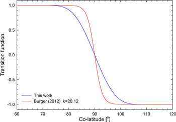
Figure 2. Transition functions as a function of colatitude, assuming a proton rigidity of 0.1 GV at 1 au, for a flat current sheet. Blue line denotes  from this study (Equation (6)), red line the Burger (2012) transition function. See the text for details.
Download figure:
Standard image High-resolution imageSubstituting Equation (5) into (1) in the same manner as done by Burger (2012) then leads to

with the first term representing the contribution due to gradient and curvature drift, and the second, the contribution of HCS drift. As the first term is essentially identical to that of Burger (2012), in what follows the emphasis shall be placed on the behavior of the second term. In order to compare with the theoretical average drift speed calculated by Burger (1987) and Burger et al. (1987), a flat current sheet, a weak-scattering drift coefficient, and a Parker field are assumed, so that the drift velocity due to HCS drift becomes
where  denotes the first derivative of S (Equation (8)) to δ, and ψ the HMF winding angle. For the angular region of interest (
![$\theta \in [\pi /2-2{R}_{L}/r,\pi /2+2{R}_{L}/r]$](https://content.cld.iop.org/journals/2041-8205/884/2/L54/revision1/apjlab4ad6ieqn10.gif) ), the term π/2 − θ remains relatively small, such that
), the term π/2 − θ remains relatively small, such that  . Performing a θ and ϕ average over a θ interval of
  , such that
which to leading order evaluates to  , regardless of RL or r. This small deviation informs the choice of Equation (8) instead of a lower-order smoothstep function, as the use of such a function would lead to a considerably larger deviation. For example, use of the smootherstep function employed in the study of Battarbee et al. (2017) would result in a ∼21% deviation from v/6.
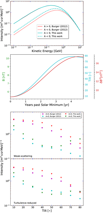
To compare and test the effects of employing the approach proposed in this work with those of using the Burger (2012) approach on GCR intensities computed using a CR modulation code, we employ the stochastic 3D simplified ab initio modulation code of Moloto et al. (2018), which is based on that of Engelbrecht & Burger (2015). This code has been demonstrated to yield results in reasonable to good agreement with galactic CR proton intensities at Earth for several successive solar minima, and utilizes the parallel and perpendicular diffusion coefficients employed by Burger et al. (2008). The turbulence-reduced drift coefficient here, however, is modeled according to the more recent approach proposed by Engelbrecht et al. (2017). For the spatial dependences of the turbulence quantities that these coefficients are functions of, e.g., the magnetic variance, simple power-law scalings as discussed by Burger et al. (2008) are employed. For the purposes of demonstration a 100 au modulation volume is assumed, using the Burger et al. (2008) boundary spectrum, and assuming a Parker (1958) HMF. Note that no attempt is made to fit observations, as only relative effects are to be discussed here, and that for the Burger (2012) runs the third term in Equation (3) is neglected. The top panel of Figure 3 shows the results of this comparison, in terms of galactic CR proton differential intensities at Earth as a function of kinetic energy. For positive magnetic polarity conditions (A > 0), both approaches yield identical results. During A < 0 there is a fair difference in intensities, with the Burger (2012) approach yielding smaller intensities. The question arises as to whether the new approach to modeling drift velocities can accurately model drift effects during periods of higher solar activity, when tilt angles are large. To test this, simple generic temporal scalings were employed for various heliospheric parameters known to vary with solar cycle, in a manner similar to that employed by Kota & Jokipii (1983). The solar cycle dependence of the tilt angle is modeled following Burger et al. (2008), while the magnetic variance and HMF magnitude at Earth are modeled using sinusoidal functions that smoothly increase by a factor of two up to solar maximum. This latter scaling is motivated by the observations reported by Zhao et al. (2018). These functions are shown in the middle panel of Figure 3, as a function of years after solar minimum. Note that the magnetic field and variance are assumed to scale in the same way with time, and are thus indistinguishable in the figure. Note also that we do not attempt to model magnetic polarity changes. The modulation code was run successively for each year after solar minimum. This approach is similar to that taken by Raath et al. (2015) when studying galactic CR intensities as a function of tilt, but differs from that study in that the HMF magnitude is here allowed to increase with increasing solar activity, and that this study does not apply essentially ad hoc expressions for diffusion and drift coefficients.
Figure 3. Top panel: galactic cosmic-ray proton differential intensities at 1 au as a function of kinetic energy computed using the Moloto et al. (2018) 3D, ab initio modulation code. Red lines correspond to solutions computed using the Burger (2012) expression for the drift velocity (Equation (3)), and teal lines to those computed using the approach outlined in this work (Equation (9)). Middle panel: temporal scalings assumed in the present study for the tilt angle (teal line) and the HMF magnitude and magnetic variance at Earth (red line). Note that the magnetic field and variance are assumed to scale similarly with time. Bottom panel: 1 GeV galactic proton intensities calculated using the approach of Burger (2012) as well as that outlined in this work, as a function of tilt angle for weak-scattering and turbulence-reduced drift coefficents.
Download figure:
Standard image High-resolution image
The bottom panel of Figure 3 shows 1 GeV galactic proton intensities calculated thus, as a function of tilt angle, for weak-scattering as well as turbulence-reduced drift coefficients. At small tilt angles, the A > 0 results are almost identical, as in the top panel of the figure, but diverge at intermediate tilt angles. This is due to the fact that, for larger tilt angles, the particles do encounter the current sheet, and thus are affected by the choice of the drift velocity modeling approach. At the highest tilt angles, both approaches yield different results, but when turbulence-reduced drift coefficients are employed both approaches yield similar intensities, due to the fact that the Engelbrecht et al. (2017) drift coefficient is reduced due to increasing turbulence levels. During A < 0 conditions and at low tilt angles, the Burger (2012) approach yields smaller intensities for both drift coefficients, and for the weak-scattering coefficient this behavior continues to the highest tilt angles considered. For the turbulence-reduced coefficients, between 30° and 60° this is no longer the case, and at the highest tilt angles the approach proposed here yields intensities that increase steadily until they are approximately equal to the A > 0 intensities at 80° tilt, while the results calculated using the Burger (2012) approach do not. This behavior is again due to the turbulence-reduced drift coefficient, but in the case of the drift approach proposed in this study is now also influenced by the reduction of the efficacy of the current sheet due to the decrease in proton Larmor radius resulting from the increased HMF magnitude. For the weak-scattering coefficients, both approaches yield intensities very different to the corresponding A > 0 values, which is not surprising, as the use of such a drift coefficient leads to a general overestimation of drift effects at solar maximum (see, e.g., Burger et al. 2000; Ferreira et al. 2003). Overall, with turbulence-reduced drift coefficients, both approaches yield results qualitatively in agreement with the observed intensity-tilt observations reported by Lockwood & Webber (2005), but only the approach proposed here leads to similar intensities for both A > 0 and A < 0 at the highest tilt angles, in agreement with observations (see, e.g., Zhang 2003) and previous simulations (e.g., Ferreira et al. 2003).
3. Summary and Conclusions
The approach to modeling particle drift velocities outlined here provides a relatively simple, numerically cost-effective way to incorporate the physics of drift into numerical solar energetic particle transport models, and has been demonstrated to yield results very similar to those computed using the Burger (2012) approach when implemented in an ab initio GCR modulation code. Furthermore, the current approach also serves to limit some uncertainties in the Burger (2012) approach. The drift speed in the present approach always remains below the particle speed. The new approach to modeling drift velocities was also incorporated into an existing CR modulation code, and galactic CR differential intensities calculated at Earth and compared with those calculated using the Burger (2012) approach, assuming heliospheric conditions corresponding to generic solar minimum and ascending to generic solar maximum conditions. During full solar minimum, both approaches yield very similar differential intensity spectra during A > 0, with the Burger (2012) approach yielding smaller intensities during A < 0. Both approaches yield results that qualitatively reproduce the observed behavior of galactic proton intensities as a function of tilt angle, but only the new approach yields results that are almost identical for both positive and negative magnetic polarity conditions at the highest tilt angle considered when turbulence-reduced drift coefficients are employed, which is in line with observations.
Additionally, modeling drift velocities in the manner outlined here will greatly facilitate the inclusion of long-lived multiple current sheet structures, as observed by, e.g., Khabarova et al. (2017) and possibly due to the multipole structure of the HMF at times of greater solar activity (e.g., Bravo & Gonzalez-Esparza 2000; Sanderson et al. 2003; Kislov et al. 2019), into numerical CR transport models. This can simply be done by defining multiple current sheets, and specifying unique transition functions for each such structure.
Future work will focus on a careful comparison of drift effects calculated using the current approach as well as those outlined by Burger et al. (1985) and Burger (2012) over an entire solar cycle.
This work is based on the research supported in part by the National Research Foundation of South Africa (grant No. 111731). S.E.S. Ferreira acknowledges support from the National Research Foundation of South Africa (grant No. 109253). Opinions expressed and conclusions arrived at are those of the authors and are not necessarily to be attributed to the NRF.
N.E.E. would like to thank K.D. Moloto for useful discussions related to this study.