


ABSTRACT
Analysis of particle-in-cell simulations of kinetic plasma turbulence reveals a connection between the strength of cascade, the total heating rate, and the partitioning of dissipated energy into proton heating and electron heating. A von Karman scaling of the cascade rate explains the total heating across several families of simulations. The proton to electron heating ratio increases in proportion to total heating. We argue that the ratio of gyroperiod to nonlinear turnover time at the ion kinetic scales controls the ratio of proton and electron heating. The proposed scaling is consistent with simulations.
Export citation and abstract BibTeX RIS
1. INTRODUCTION
The nature of the nonlinear energy cascade and its effects on thermal properties of turbulent plasma are central problems in understanding the heating of the solar corona, the origin of the solar wind, and numerous other problems in space physics (Matthaeus & Velli 2011). The same fundamental physics issues are broadly relevant in turbulent astrophysical plasmas (Lazarian et al. 2012) and enter in diverse circumstances including molecular clouds, where turbulent heating influences star formation (Mac Low 1999) and cooling flows where turbulent fluctuations regulate heat transport (Chandran & Cowley 1998; Banerjee & Sharma 2014). A standard turbulence scenario inherited from hydrodynamics and magnetohydrodynamics (MHD) at high Reynolds numbers emphasizes a power-law inertial range spectrum that describes the steady distribution of energy across scales, a matter of great importance, e.g., in the resonant scattering of energetic particles (Jokipii 1966). However, that the inertial range acts as a near-lossless conduit that connects energy-containing large scales to the dissipative small scales is of equal importance. This energy transfer across scales in effect "completes" the circuit that allows a system far from equilibrium to relax toward thermal equilibrium. In sufficiently large hydrodynamic and MHD systems, it is widely recognized that the energy-containing eddies control the rate of transfer into the inertial range and therefore control the dissipation rate, on average. For a kinetic plasma, the theoretical understanding is less developed and perhaps more controversial, but there is also accumulating evidence that large-scale reservoirs of energy exert and regulate the rate of relaxation, fueling the the response of the plasma physics at much smaller scales, leading eventually to dissipation (Karimabadi et al. 2013). The present study further elucidates the kinetic plasma cascade process, focusing on the same two energy fluxes: the flux into the inertial range and the flux into dissipation channels. We proceed based on empirical evidence from simulations, extending an earlier preliminary report (Wu et al. 2013). Progress on these issues will lead to a better understanding of heating and other crucial effects of turbulence in space and astrophysical applications.
2. LARGE-SCALE TURBULENCE DRIVES HEATING
The standard von Karman approach to computing turbulent decay rates (de Kármán & Howarth 1938) may be adapted to MHD (Hossain et al. 1995; Wan et al. 2012). A similarity-law decay rate, written in terms of the Elsässer amplitudes  and
and  and their respective similarity length scales
  and
and  , may be written as
  .
.  and
and  are von Karman constants that may depend on other parameters. A simplified version, often employed when normalized cross helicity
  is near zero, is
  containing a single correlation scale λ and a single von Karman constant CK. Adopting the latter for simplicity, the decay rate at large scales is related to the dissipation and the rate of heating as

Here, protons and electrons are the only species present, and Qp and Qe are their respective heating functions, or local rates of addition of internal energy.
Note that we write the von Karman "constant" as  to emphasize that it is expected to depend on parameters such as cross helicity, plasma beta, and the ratio of kinetic to magnetic energy as well as Reynolds number or system size. Figure 1 shows the total heating rate
  , obtained as the average rate of temperature increase for each species, as a function of von Karman decay rate
  , for each run in Table 1. To compute the (time-averaged) heating rates from the simulations, we evaluated the change in the temperature over a period of five nonlinear times and divide by that time interval to give thermal energy input per nonlinear time. That is, e.g., for protons,
  (where τnl is the global nonlinear time; see below), and similarly for electrons. Within each family of runs a linear relationship is apparent, indicating a residual dependence on other parameters in the von Karman constant, which can be accommodated in the parametric dependence of
  as anticipated above. (Such parameters are constant within each family.) This result further strengthens the conclusions of Wu et al. (2013) in affirming the applicability of the von Karman average decay rate. In that earlier work the approach was somewhat different, examining the temporal dependence of the fluctuation energy decay rate normalized to its von Karman value, the full version of which is given just above Equation (1). Note that the runs other than Orszag-Tang runs employed in the present study (see Table 1) have low cross-helicity (
 ) and comparable length scales
  for the two Elsässer fields; therefore, the simplified form of
  given in Equation (1) is relevant.
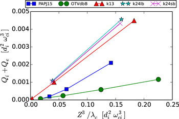
Figure 1. Scaling of total heating rate  with the estimated decay rate
  .
.  computed from average temperature increase during the first 5 nonlinear times. See Table 1 for Run family names. The smallest system size from Parashar et al. (2015) is omitted as it was is an extreme outlier, too small for MHD-like behavior.
Download figure:
Standard image High-resolution imageTable 1. Properties of Simulation Runs
| Run | Family | βi | βe | Z0 | B0 | λc | L | Nx = Ny | Qi/Qe | τc/τnl | ppg | k |
|---|---|---|---|---|---|---|---|---|---|---|---|---|
| run805.1 | PAPJ15 | 0.08 | 0.08 | 3.131 | 5.0 | 0.446 | 1.28 | 64 | 0.584 | 0.820 | 200 | {1, 2} |
| run805.2 | PAPJ15 | 0.08 | 0.08 | 2.334 | 5.0 | 0.717 | 2.56 | 128 | 0.887 | 0.521 | 200 | {1, 2} |
| run805.3 | PAPJ15 | 0.08 | 0.08 | 2.085 | 5.0 | 1.143 | 5.12 | 256 | 0.435 | 0.399 | 200 | {1, 2} |
| run805.4 | PAPJ15 | 0.08 | 0.08 | 2.017 | 5.0 | 1.971 | 10.24 | 512 | 0.331 | 0.322 | 200 | {1, 2} |
| run805.5 | PAPJ15 | 0.08 | 0.08 | 2.000 | 5.0 | 3.627 | 20.48 | 1024 | 0.343 | 0.260 | 200 | {1, 2} |
| run809.1 | OTVdbB | 0.08 | 0.08 | 2.031 | 5.0 | 3.820 | 20.48 | 1024 | 0.551 | 0.260 | 200 | {1, 2} |
| run810.1 | OTVdbB | 0.08 | 0.08 | 3.041 | 5.0 | 3.928 | 20.48 | 1024 | 0.588 | 0.385 | 200 | {1, 2} |
| run811.1 | OTVdbB | 0.08 | 0.08 | 4.052 | 5.0 | 4.286 | 20.48 | 1024 | 0.754 | 0.499 | 200 | {1, 2} |
| run812.1 | OTVdbB | 0.08 | 0.08 | 5.064 | 5.0 | 4.608 | 20.48 | 1024 | 0.945 | 0.609 | 200 | {1, 2} |
| Turb808 | k13 | 0.25 | 0.25 | 0.986 | 5.0 | 2.842 | 25.6 | 2048 | 0.404 | 0.139 | 400 | {1, 3} |
| Turb812 | k13 | 0.25 | 0.25 | 2.464 | 5.0 | 2.886 | 25.6 | 2048 | 0.542 | 0.346 | 400 | {1, 3} |
| Turb813 | k13 | 0.25 | 0.25 | 3.942 | 5.0 | 2.685 | 25.6 | 2048 | 0.857 | 0.567 | 400 | {1, 3} |
| Turb814 | k24lb | 0.25 | 0.25 | 2.456 | 5.0 | 3.069 | 25.6 | 2048 | 0.697 | 0.338 | 400 | {2, 4} |
| Turb815 | k24lb | 0.25 | 0.25 | 3.930 | 5.0 | 3.030 | 25.6 | 2048 | 1.159 | 0.543 | 400 | {2, 4} |
| Turb816 | k24sb | 0.10 | 0.10 | 2.456 | 5.0 | 3.106 | 25.6 | 2048 | 0.546 | 0.337 | 400 | {2, 4} |
| Turb817 | k24sb | 0.10 | 0.10 | 3.930 | 5.0 | 3.075 | 25.6 | 2048 | 1.010 | 0.541 | 400 | {2, 4} |
Note. All simulations employ P3D particle-in-cell code in 2.5D (three components for vectors; two-dimensional grid) periodic boxes of lengths described in the L column and the grid described in the Nx = Ny column. This table does not list the runs from Wu et al. (2013). Listed are proton beta  , electron beta
  , turbulence amplitude Z0, out of plane unfirm magnetic field B0, correlation scale
  , box size L, grid points in plane Nx = Ny, the ratio of average ion/electron heating rates
  , the ratio of proton cyclotron time to nonlinear time at di ion inertial scale
  , the number of particles per grid point ppg and the wavenumber band of initial conditions. All lengths are in di. The b and v fluctuations in the initial conditions were excited for wavenumbers having the values given in the k column and with a given initial spectrum. The time step in all the simulations was chosen to satisfy the CFL condition for the speed of light.
Download table as: ASCIITypeset image
3. PROTON RESPONSE TO STRONGER CASCADE
We now direct our attention to the question of how the proton heating responds to the strength of the cascade. More specifically, we will examine how the ratio of heating rates  varies with the total cascade rate, as measured by the total heating rate
  . Before presenting new results, we call attention to several suggestions made in the recent literature.
An important clue comes from the observational study of solar wind data (Smith et al. 2006), which found steeper sub-proton scale slopes of the magnetic energy spectrum in cases that have larger estimated cascade rates. The suggestion was that a more robust turbulence cascade at larger MHD scales leads to greater dynamical response by thermal protons. A subsequent solar wind observational study (Matthaeus et al. 2008) bolstered this conclusion by examining the influence of the cascade rate on Taylor microscale  , which is a measure of the root mean square curvature of the magnetic field. For smaller cascade rates,
  can actually be smaller than the ion inertial scale di, while for large cascade rates
  . To interpret this, one may note that the hydrodynamic ordering of Taylor and dissipation scale η is always
  . Then, if one associates the "steepening scale" of the solar wind magnetic spectrum with di, the suggestion emerges that the magnetic field is more greatly smoothed by processes active at scales near di when the cascade rate is larger.
Based on the above reasoning, the working hypothesis becomes that dissipation is enhanced near protons scales when the total dissipation rate is greater. This is basically because larger cascade rate in a Kolmogorov-style cascade increases the small scale fluctuations. In particular, the typical component magnetic increments  at scale ℓ behave as
  , so it is apparent that for ion scales
  , the fluctuations will increase as
  . This causes a greater perturbation to proton orbits, which will increase the heating of protons. It also leaves less energy in the sub-proton scale cascade, resulting in less heating of electrons. At large fluctuation amplitude we expect that the relative heating of protons should saturate at some value. We may formulate this expectation as

the former of which will be subject to saturation at large amplitude, while the second relation remains accurate on average. These relations are directly testable in kinetic plasma simulation. Using the same ensemble of simulations described in Table 1, we tested this hypothesis; the results are illustrated in Figure 2. There is considerable scatter in this figure, in part due to the fact that these runs are from different families of initial conditions. However, it is apparent that there is a general trend for increased relative relative heating of protons compared to heating of electrons in runs that have larger total heating. This result is consistent with the findings of Wu et al. (2013).
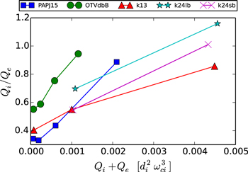
Figure 2. Scaling of relative proton–electron heating  with total heating rate
  . As expected the relative heating of protons increases with the total heating rate. See the remark at the end of the Figure 1 caption.
Download figure:
Standard image High-resolution image4. CONNECTION OF PROTON HEATING TO TIMESCALES
To have an effective transfer of energy between collective fluid scales and random thermal motions of particles in a magnetized plasma, one must either energize particles in the parallel (to magnetic field) direction or disrupt the perpendicular gyromotion. Parallel energization is most easily accomplished in current channels in which there are low levels of transverse magnetic fluctuations. This process is obviously more effective for electrons, given their smaller gyroradius, and has been documented for test particle electrons in MHD turbulence and in kinetic simulations (Dmitruk et al. 2004; Drake et al. 2006). This type of parallel energization of protons may also occur, but will tend to operate at lower energies. Disruption of perpendicular gyromotion is necessary to break the adiabatic invariance of magnetic moment (see e.g., Chandran et al. 2010). The effectiveness of this disruption depends on the degree to which the magnetic field at the scale of the particle gyro-orbit changes during a gyroperiod. In turbulence, the magnetic field moving with the material elements (here, the ExB drift velocity) is reconfigured over a timescale given by the nonlinear time  at the relevant scale ℓ. Therefore, the fractional reconfiguration in a gyration timescale
  (total rms magnetic field
  including mean and fluctuations) is given by
  .
.
The scale-dependent nonlinear time may be evaluated from standard von Karman–Kolmogorov phenomenology. The large-scale or global nonlinear time is  , where Z is the mean turbulence amplitude and λ the correlation or energy-containing scale. (Again, for simplicity, we specialize to zero- or low-cross helicity and a single length scale.) Then, one estimates the turbulence amplitude at smaller inertial range scales as ℓ given by
  , consistent with both the 1941 and 1962 Kolmogorov inertial range scalings. The nonlinear timescale at ℓ is
  .
.
The simplest choice for ℓ is the ion inertial scale di, which has often been associated with the spectral break observed in the solar wind (Leamon et al. 1998) as well as current sheet thicknesses in plasma simulations (Shay et al. 1998) and in laboratory experiments (Brown et al. 2006). However, there are also reasonable arguments for selecting the thermal gyroradius  as the relevant length scale for heating and we will discuss this below. For now, we adopt the hypothesis the heating of protons is sensitive to the nonlinear timescale at the ion inertial scale and in the simulation database we empirically test the hypothesis that

Note that the last factor is related to system size. Furthermore, if one associates the ion inertial scale with the turbulence Kolmogorov dissipation scale η, then effective Reynolds number is  and Equation (3) is equivalent to
  .
.
Figure 3 shows the scaling of relative proton–electron heating with  according to the above hypothesis. Note that this ratio was also discussed by Matthaeus et al. (2014) as a useful measure of the influence of turbulence on kinetic processes such as linear Vlasov waves and linearized damping rates, which arguably require relatively undisturbed conditions for attaining their assumptions. Here, we are examining the complementary situation in which the disturbance of gyromotion by turbulent reconfiguration at ion scales is expected to promote proton heating. Note that the data plotted has many PIC simulations, including simulations in (Wu et al. 2013). We clearly observe that
  increases with
  , supporting the hypothesis in Equation (3).
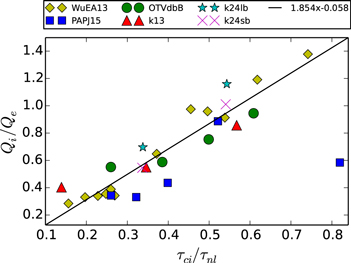
Figure 3. Scaling of relative proton–electron heating  with the estimated ratio
  of cyclotron time to nonlinear time evaluated at the ion inertial scale. In this figure, the outlier point on the right is the smallest system from Parashar et al. (2015), which does not have any signs of MHD-like or von Karman-like behavior.
Download figure:
Standard image High-resolution image5. ASSOCIATION OF HEATING WITH SPATIAL STRUCTURES
The statistics examined so far have not specifically emphasized the role of coherent structures in the proton heating processes, yet theory indicates that coherent structures in the magnetic and plasma flow (Dmitruk et al. 2004; Markovskii et al. 2006; Parashar et al. 2011; Dalena et al. 2014; Wan et al. 2015) play an important role, as is confirmed in observations (Retinò et al. 2007; Osman et al. 2011). In particular, substantial fractions of heating are known to occur in boundary layer-like regions within or near proton scale current sheets (Ambrosiano et al. 1988; Dmitruk et al. 2004; Dalena et al. 2012; Drake et al. 2014). These structures typically have one or more dimensions on the order of an ion inertial scale (Dmitruk & Matthaeus 2006; Markovskii & Vasquez 2011; Wang et al. 2013; Makwana et al. 2015), which motivates our evaluation of the nonlinear time at di. The dynamical processes that occur in association with these structures include energization by direct (parallel) electric fields; strong scattering and confinement leading to stochastic orbits; betatron effect; and pickup by flows through  drift effect. These effects have been parameterized in various phenomenologies (Ambrosiano et al. 1988; Drake et al. 2006; le Roux et al. 2015) and it is likely that observed transfer of energy into random degrees of freedom, i.e., heating, occurs as a consequence of all of these acting in concert. The net effect of these processes, and notably their localization in structured patterns reflecting the magnetic structure of the turbulence, is evident in the simulations.
To illustrate the spatial intermittency and related properties of the heating, we plot Tp, Te,  and Jz in Figure 4. The Figure is based on run Turb817, which has
  ,
,  and
and  (see Table 1).

Figure 4. Jz,  , Tp, and Te for the run Turb817 at roughly 10 nonlinear times. Electrons are hottest at the sites of strong currents, while protons are generally hotter in areas "near" strong current structures (current sheets as well as peripheries of islands). The sites of large proton heating are also generally the sites where protons are generally hotter than electrons.
Download figure:
Standard image High-resolution imageThe electrons are hottest at the sites of strongest thin current sheets. Proton hotspots are relatively broader and are concentrated around the strong currents near magnetic "islands" and the interaction region between pairs of islands (Ambrosiano et al. 1988; Dmitruk et al. 2004; Chandran et al. 2010; Shay et al. 2014). (The hotspots where protons are hotter than electrons are mostly the spots where protons are strongly heated. These spots are the sites of strong currents around the islands.)
6. DISCUSSION: SCALING OF PROTON–ELECTRON HEATING
The above results lead to a perspective on plasma heating in which a von Karman, MHD-like heating rate is supported by highly nonuniform, intermittent dissipation processes that are related to coherent structure that form in or near boundaries at the edges of interacting magnetic flux tubes. There seems to be both a spatial and a temporal character to the conditions that favor strong proton heating. Evidently, proton heating is favored when the timescale for reconfiguration of the favored fluctuations becomes small enough that distortions occur within a gyroperiod. On the other hand the favored spatial scales are those that couple well to the proton population, i.e., the important fluctuations are those at or near the proton kinetic scales. In this way, the coupling of turbulent motions to heating might be viewed as a kind of generalization of resonance conditions; however, here with the interactions being with coherent structures rather than with wave trains and the time variations being of nonlinear origin and not simply oscillatory.
In the above analysis we employed the ion inertial scale di as the scale of interest, at which dissipative couplings to random motions occur, based on observations of the spectral breakpoints and current sheet thicknesses seen in solar wind, simulations and laboratory experiments. However, one also might have employed the thermal particle gyroradius  as the preferred scale. In that case, the relevant nonlinear timescale would be
  , where
  (sound speed cs; Alfvén speed VA). Note that with the choice of gyroradius, the theory captures a better fit to the particle population; however, employing the ion inertial scale the theory makes better contact with the expected width of boundary layers, such as current sheet thicknesses. For a more general description of proton–electron heat functions, one might like to anticipate a more general β dependence, of the form
  .
.
Based on the above analyses, we can now propose a description of proton heating:

and electron heating:

that are in accord with the theoretical and empirical descriptions given in the sections above. These prescriptions satisfy
- 1.a von Karman scaling of the total heating rate

- 2.a scaling of the heating ratio with the total heating rate;
- 3.a scaling of the proton–electron heat function ratio with the timescale ratio, the latter evaluated at a scale ℓ in the range of di or controlled by the function .


Kinetic simulations (Servidio et al. 2012; Karimabadi et al. 2013) as well as test particle studies (Dmitruk et al. 2004) have shown that temperature anisotropies occur preferentially in the vicinity of coherent structures. That issue has not been examined here, although we fully expect that association is also present in the present simulations. These simulations were carried out in 2.5D (see Table 1) to maximize available spatial resolution. Although fully 3D studies would be preferred, we note that recent study Wan et al. (2015, 2016) showed a surprising degree of similarity between dissipation statistics in 2.5 and 3D runs of several types. It is also noteworthy that our simulations clearly exhibit coherent structures and intermittency (see Figure 4) but nonetheless are of limited system size (and effective Reynolds numbers). Therefore, we would expect that in still larger simulations the role of heating in or near coherent structures would be even greater.
This research was supported by NSF AGS-1063439, AGS-1156094 (SHINE), AGS-1460130 (SHINE), NASA grants NNX14AI63G (Heliophysics Grand Challenge Theory), and the Solar Probe Plus science team (ISIS/SWRI subcontract No. D99031L).
APPENDIX:
All the simulations used in this Letter were performed using the fully electromagnetic particle in cell code P3D (Zeiler et al. 2002) in periodic 2.5D (3 component vectors on a 2D grid) geometry. Simulations in the PAPJ15 family were also used to study the approach to MHD-like behavior in kinetic plasmas in (Parashar et al. 2015). Table 1 does not list simulations used in (Wu et al. 2013). Runs in the OTVdbB family are Orszag–Tang vortex runs with varying  amplitudes. Runs in the k13, k24lb and k2sb families were performed specifically for this study. These were initialized with MHD-like v and b fluctuations (solenoidal velocity and uniform density) excited at the wavenumbers within the k band given in the table with a specified spectrum, so that the initial energy is concentrated near the largest excited wavenumbers. The energy then cascades to fill in the complete wavenumber range available and produce turbulence. Typical parameters for these runs (except for Wu et al. 2013 runs) are given in Table 1.