


Abstract
We conducted an analysis of the abundances of He, C, and N in 210 He-rich hot subdwarfs observed within both the Gaia Data Release 3 (DR3) and LAMOST DR7 data sets. This analysis involved fitting the LAMOST spectra with Tlusty/Synspec non-LTE synthetic spectra. By examining the Galactic spatial positions, velocity vectors, and orbital parameters of these stars, we determined their Galactic population memberships utilizing LAMOST radial velocities and Gaia DR3 parallaxes along with proper motions. Our investigation revealed two positive correlations of C and one positive correlation of N with respect to the He abundance. We found a clear C abundance dichotomy where approximately 82% of the stars show N enrichment above the solar value. Moreover, we observed a bimodal distribution of C abundances, prominently evident in both the Galactic thin and thick disks but absent in the halo population. Furthermore, we found that the scenario of the merger channel of double helium white dwarfs is inadequate to explain the formation of C-deficient He-rich hot subdwarfs.
Export citation and abstract BibTeX RIS

Original content from this work may be used under the terms of the Creative Commons Attribution 4.0 licence. Any further distribution of this work must maintain attribution to the author(s) and the title of the work, journal citation and DOI.
1. Introduction
Hot subdwarf stars represent highly evolved celestial objects usually found in the core helium-burning phase or beyond. Their typical mass is around 0.5 M⊙, with a radius ranging from 0.1 to 0.3 R⊙. Despite their relatively small size, their spectra closely resemble those of main-sequence O/B stars. In the Hertzsprung–Russell (H-R) diagram, hot subdwarfs are found at and beyond the very hot end of the horizontal branch. Hot subdwarfs are generally classified into three groups based on their spectral characteristics: subdwarf B (sdB), subdwarf OB (sdOB), and subdwarf O (sdO). While most hot subdwarf stars have helium-poor atmospheres, with helium abundances that can be extremely low, approximately 10% of these stars have helium-rich atmospheres. A comprehensive review of hot subdwarfs was presented by Heber (2016).
The origins of He-rich hot subdwarf stars remain enigmatic, with further classifications into extreme He-rich (eHe) and intermediate He-rich (iHe) subtypes. Proposed formation channels include the merger of two He white dwarf stars (HeWDs; Han et al. 2002, 2003) and the late hot flasher scenario (Miller Bertolami et al. 2008; Battich et al. 2018). The merger of HeWDs is considered a key scenario given the notably low fraction of He-rich hot subdwarf stars in binary systems. Their observed positions in the Kiel diagram align well with theoretical HeWD merger tracks (Zhang & Jeffery 2012). Recent studies in binary population synthesis (Yu et al. 2021) have also demonstrated that this channel could explain the various subclasses of surface carbon abundance within the observed  panel. Furthermore, the observed distribution of He-rich hot subdwarf stars within Galactic populations appears to support the scenario of two HeWD mergers (Luo et al. 2019, 2020, 2021). However, the merger of two HeWDs does not entirely elucidate the formation of both H-rich and He-rich subtypes. The late hot flasher scenario stands as another compelling hypothesis but lacks the capacity to explain the presence of surface C-deficient stars (Hirsch 2009). Other models, such as the merger of a hybrid CO/He-core WD and an He-core WD (Justham et al. 2011), have been suggested to account for the He-rich stars, but they do not encompass all He-sdB stars. Recently, Werner et al. (2022) discovered a new class of He-rich sdO stars significantly enriched in C and O (CO-sdO), possibly explained by the merger of a HeWD and a less massive CO-core WD (Miller Bertolami et al. 2022). Additionally, Dorsch et al. (2022) reported the discovery of a highly magnetic He-sdO star resulting from a double-degenerate binary merger. Subsequently, Pelisoli et al. (2022) identified three new magnetic He-rich hot subdwarf stars but was unable to precisely determine the type of merger or the surface C abundance. Therefore, additional observational constraints are needed to refine existing models.
The advent of the Gaia and LAMOST low-resolution surveys (LRS) has provided invaluable insights into the formation pathways of He-rich subdwarf stars. Through a comprehensive analysis of the kinematics and spectroscopic properties within substantially large observed samples, we have been able to impose observational constraints on these formation channels. Utilizing data from Gaia Data Release 2 (DR2) and LAMOST DR5, Luo et al. (2019) have unveiled the fractional distributions of two distinct He-rich subdwarf groups (eHe and iHe) within the Galactic halo, thin-disk, and thick-disk populations. Our findings suggest that eHe subdwarf stars likely originate from mergers of binary HeWDs, while the principal formation channels for iHe subdwarfs may not necessarily involve the mergers of HeWDs with low-mass main-sequence stars. In our most recent study, we (Luo et al. 2021) identified 1578 hot subdwarf stars from the Gaia DR2 catalog of hot subdwarf star candidates with spectra available in LAMOST DR7. The investigation distinguished two eHe groups (eHe-1 and eHe-2) and two iHe groups (iHe-1 and iHe-2). The kinematic analysis revealed that over half of the stars in group eHe-1 belong to the thick-disk population, while over half of the stars in group eHe-2 are associated with the thin disk. Two possible scenarios—the merger of two HeWDs (Zhang & Jeffery 2012) and the late hot flasher scenario (Miller Bertolami et al. 2008; Battich et al. 2018)—have predicted observable differences in the C and N abundances. However, our previous investigations (Luo et al. 2019, 2021) focused solely on analyzing hydrogen and helium abundances, without exploring the C and N abundances.
This paper aims to analyze the C and N abundances, along with the kinematics, of 210 He-rich subdwarf stars observed in Gaia DR3 and LAMOST DR7 to gain insights into their formation. Section 2 describes the sample selection process and data. Section 3 presents the spectral analysis and classification within the Galactic populations. Section 4 encompasses the results and discussions. Finally, Section 5 summarizes our conclusions.
2. Sample Selection and Data
2.1. Sample Selection
The sample studied in this investigation was derived from the catalogs of spectroscopically identified hot subdwarf stars listed in Gaia DR2, combined with spectra from LAMOST survey releases DR5, DR6, and DR7 (Lei et al. 2018, 2019,2020; Luo et al. 2019, 2021). Initially, 350 He-rich hot subdwarf stars were collected from these catalogs. Subsequently, the sample was expanded to encompass entries from the catalog of known hot subdwarf stars (Geier 2020), which provides crucial spectroscopic parameters such as effective temperatures, surface gravities, and helium abundances for 2187 hot subdwarf stars. Cross-referencing this catalog with LAMOST DR7 led to the inclusion of an additional 41 He-rich hot subdwarf stars in the analyzed sample.
After crossmatching the selected sample from Gaia DR3 and LAMOST DR7, a total of 391 He-rich hot subdwarf stars were identified in both Gaia DR3 and LAMOST DR7. To investigate C and N abundances, the final sample was refined to include 210 He-rich hot subdwarf stars with LAMOST spectra having a signal-to-noise ratio (S/N) greater than 25 in the g band. Figure 1 shows the positions of this sample in the Gaia H-R diagram.
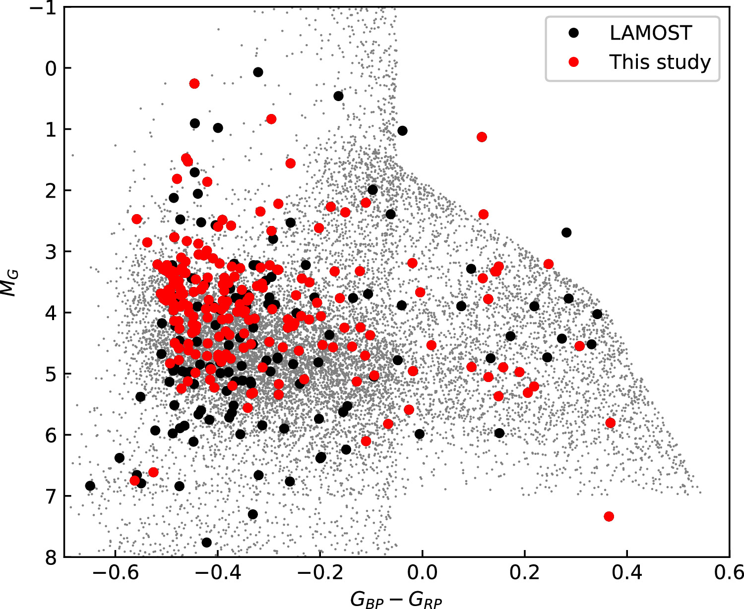
Figure 1. The H-R diagram of stars selected from the Gaia DR2 hot subdwarf candidate catalog. The black dots represent all known He-rich hot subdwarf stars observed in LAMOST DR7, with the red dots specifically highlighting LAMOST spectra having S/N > 25 in the g band.
Download figure:
Standard image High-resolution imageIn our previous work (Luo et al. 2021), we demonstrated that hot subdwarf stars observed in the LAMOST DR7 and Gaia DR2 samples, located between 500 and 1500 pc away, exhibit a very similar distribution function in their absolute Gaia magnitudes. We proposed that the LAMOST DR7 hot subdwarf star sample is a representative and unbiased subsample of the volume-complete Gaia sample. Figure 2 illustrates the nearly identical distribution functions for all He-rich hot subdwarfs in LAMOST DR7 and our final sample concerning absolute Gaia magnitudes (MG) and distances.
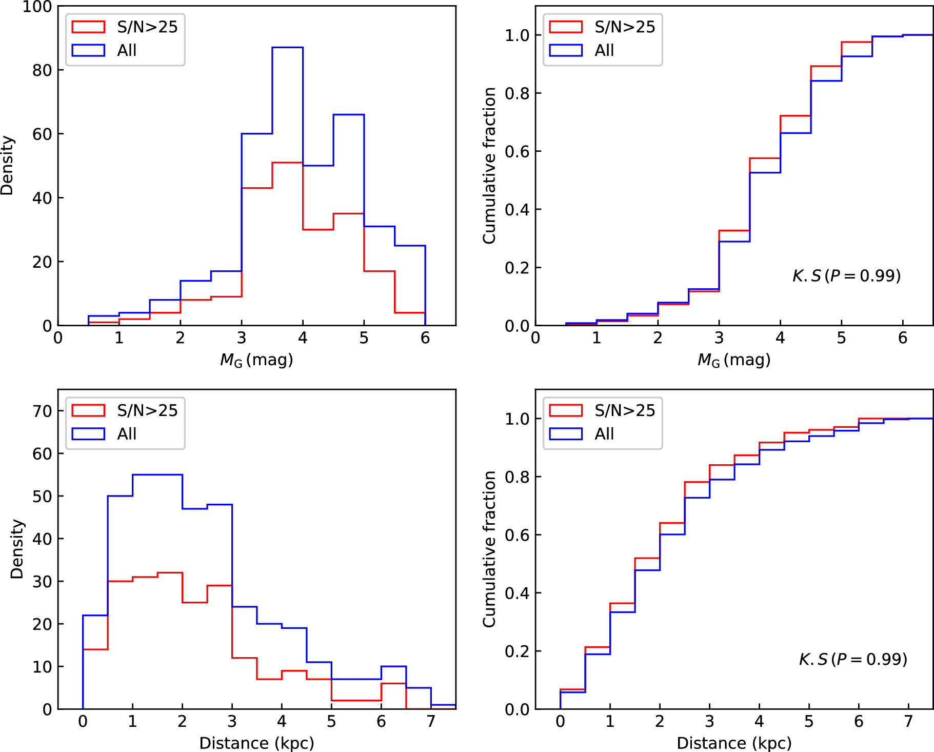
Figure 2. Comparisons of the density and cumulative distribution functions of the Gaia absolute G magnitude MG and distances between our sample and all LAMOST He-rich samples.
Download figure:
Standard image High-resolution image2.2. Spectral Data
We utilized the spectra from LAMOST DR7 to determine the atmospheric parameters of the selected objects. These parameters include effective temperature Teff, surface gravity  , He abundance
  , C abundance
  , and N abundance
  and radial velocity. The LAMOST spectra, akin to Sloan Digital Sky Survey data, have a spectral resolution of R ∼ 1800 and cover a wavelength range from 3750 to 9100 Å. More detailed information about the data can be found at http://www.lamost.org/dr7/v2.0/.
Gaia DR3 (Gaia Collaboration et al. 2023) provided precise positions (α and δ), proper motions ( and μδ
), and parallaxes (
and μδ
), and parallaxes ( ), as well as three broadband magnitudes (G, GBP, and GRP) for all 210 He-rich hot subdwarf stars. Distances (D) were computed by simply inverting the parallax. For two stars with unreliable parallaxes and 48 stars with a parallax_over_error < 5, their distances were substituted with the estimated values from the Gaia DR3 distance catalog (Bailer-Jones et al. 2021).
3. Spectral Analysis and Galactic Population Classification
3.1. Spectral Analysis
Atmospheric parameters were derived by fitting non–local thermodynamic equilibrium Tlusty (v207) and Synspec (v53) (Hubeny & Lanz 1995, 2017) models to LAMOST spectra. We employed the iterative data-driven spectral analysis procedure XTgrid (Németh et al. 2012) to optimize all free parameters simultaneously and determine the most suitable parameter values that provide the best fit. The models included H, He, C, and N chemical elements self-consistently in both the atmospheric model calculations and spectrum synthesis. Details regarding the ionization stages for which detailed model atoms are used in the atmospheric model calculations can be found in Table 1. To ascertain the effective temperature and surface gravity and concurrently look for the abundances of He, C, and N, we employed a global minimization without individually tracing the surface parameters or the ionization balance of separate ions. The global minimization assumes that a single model is able to reproduce the observation. This approach ensures that all parameter correlations and interconnections are considered. However, at the same time, it is sensitive to inconsistencies in or a lack of atomic data, which becomes apparent only in the hottest stars of our sample. Figure 3 shows a global fit to a single spectrum, and Figure 4 displays fits to the LAMOST LRS spectra of eight hot subdwarf stars with Teff ranging from 30,000 to 51,000 K. The LAMOST LRS observations encompass most of the reliable diagnostic lines of the He, C, and N ions.

Figure 3. LAMOST LRS spectrum of J024734.99+364550.3 (black) and the final model (red) with He (magenta), C (blue), and N (green) lines.
Download figure:
Standard image High-resolution image
Figure 4. Best-fit Tlusty/XTgrid models (red) for the LAMOST LRS spectra of eight hot subdwarf stars (gray) with Teff ranging from 30,000 to 51,000 K. All fits were done on the flux-calibrated observed spectra and renormalized along with the models for a better representation. The major H, He, C, and N lines that dominated the chi-square during the fits are marked.
Download figure:
Standard image High-resolution imageTable 1. Ionization Stages for Which Detailed Model Atoms Were Utilized in the Model Atmosphere Calculations with Tlusty/Synspec
| Element | L | SL | Element | L | SL | Element | L | SL | Element | L | SL |
|---|---|---|---|---|---|---|---|---|---|---|---|
| H | 16 | 1 | He i | 24 | 0 | C ii | 34 | 5 | N ii | 32 | 10 |
| ⋯ | ⋯ | ⋯ | He ii | 20 | 0 | C iii | 34 | 12 | N iii | 39 | 9 |
| ⋯ | ⋯ | ⋯ | ⋯ | ⋯ | 0 | C iv | 35 | 2 | N iv | 34 | 14 |
| ⋯ | ⋯ | ⋯ | ⋯ | ⋯ | 0 | ⋯ | ⋯ | ⋯ | N v | 21 | 4 |
Note. The number of levels (L) and superlevels (SL) are provided. For each atom/ion, the ground state of the next higher ionization stage was also included, although it is not listed here.
Download table as: ASCIITypeset image
All models were calculated in real time, adjusting the model parameters through comparison of the synthetic spectra with the observed spectra within the 3780–6850 Å wavelength range. The synthetic spectra were convolved with an instrumental profile to match the resolution of the LAMOST data and normalized to the flux of the LAMOST spectra within 80 Å segments. Additionally, the radial velocity was determined by measuring the Doppler shift between the observed data and the model.
As also described by Schindewolf et al. (2018), many C and/or N lines are blended with He lines in He-rich hot subdwarfs. Metal lines are often occurring in the wings of H/He lines (see Figure 3), and these overlaps significantly impact the determination of the atmospheric parameters from low-resolution spectroscopy such as the LAMOST LRS. Table 2 lists the spectral lines that contributed the most in determining the atmospheric parameters. In instances when multiple ionization stages are present, such as the occurrence of both C ii and C iii lines, the fitting of these lines yields crucial insights into the C abundance and the atmospheric conditions, particularly of Teff stratification.
Table 2. List of Spectral Lines with the Largest Contributions to the Determination of Atmospheric Parameters
| Line (Å) | Line (Å) | Line (Å) | Line (Å) | Line (Å) |
|---|---|---|---|---|
| He i 3805.74 | C iii 3883.82 | C ii 5661.89 | N iii 3934.50 | N ii 5016.38 |
| He i 3809.10 | C iii 3889.14 | C iii 5771.66 | N iii 3938.51 | N ii 5045.10 |
| He i 3819.60 | C ii 3918.97 | C iv 5801.35 | N ii 3995.00 | N iii 5058.73 |
| He i 3833.55 | C ii 3920.68 | C iii 5826.42 | N iii 3998.63 | N iii 5058.96 |
| H i 3835.38 | C iii 4067.94 | C ii 5889.78 | N iii 4003.58 | N iii 5147.87 |
| He i 3838.10 | C iii 4068.92 | C ii 5891.60 | N ii 4035.08 | N iii 5320.87 |
| He i 3867.47 | C iii 4070.26 | C iii 5894.07 | N ii 4041.31 | N iii 5327.19 |
| He i 3871.79 | C ii 4074.84 | C ii 6095.29 | N iii 4097.36 | N ii 5666.63 |
| He i 3878.18 | C ii 4075.85 | C ii 6151.27 | N ii 4176.16 | N ii 5676.02 |
| He i 3888.65 | C iii 4121.85 | C ii 6461.95 | N iii 4195.74 | N ii 5679.56 |
| H i 3889.05 | C iii 4152.51 | C ii 6578.05 | N iii 4200.07 | N ii 5710.77 |
| He i 3926.54 | C iii 4156.50 | C ii 6582.88 | N ii 4236.93 | N ii 5931.78 |
| He i 3935.91 | C iii 4162.88 | C iii 6731.04 | N ii 4237.05 | N ii 5941.65 |
| He i 3964.73 | C iii 4186.90 | C iii 6744.39 | N ii 4241.79 | N iii 6467.02 |
| He ii 3968.44 | C ii 4267.26 | C ii 6750.54 | N iii 4332.95 | N ii 6482.05 |
| H i 3970.07 | C iii 4325.56 | C ii 6779.94 | N iii 4345.81 | N ii6610.56 |
| He i 4009.26 | C iii 4361.78 | C ii 6780.59 | N iii 4378.99 | ⋯ |
| He i 4023.97 | C ii 4374.28 | C ii 6783.91 | N ii 4432.74 | ⋯ |
| He ii 4025.61 | C iii 4388.02 | C ii 6787.21 | N ii 4447.03 | ⋯ |
| He i 4026.19 | C ii 4411.15 | C ii 6791.47 | N iii 4510.88 | ⋯ |
| He ii 4100.05 | C iii 4515.81 | C ii 6800.69 | N iii 4518.14 | ⋯ |
| He i 4120.81 | C iii 4516.79 | ⋯ | N iii 4523.56 | ⋯ |
| He i 4143.76 | C iii 4593.29 | ⋯ | N iii 4534.58 | ⋯ |
| He ii 4199.84 | C ii 4619.25 | ⋯ | N iii 4535.05 | ⋯ |
| He ii 4338.68 | C iii 4647.42 | ⋯ | N iii 4546.33 | ⋯ |
| H i 4340.46 | C iii 4650.25 | ⋯ | N ii 4601.48 | ⋯ |
| He i 4387.93 | C iii 4651.47 | ⋯ | N ii 4607.15 | ⋯ |
| He i 4437.55 | C iii 4652.05 | ⋯ | N iii 4610.55 | ⋯ |
| He i 4471.49 | C iv 4657.55 | ⋯ | N ii 4630.54 | ⋯ |
| He ii 4541.59 | C iii 4659.06 | ⋯ | N iii 4634.13 | ⋯ |
| He ii 4685.70 | C iii 4663.64 | ⋯ | N iii 4640.64 | ⋯ |
| He i 4713.14 | C iii 4665.86 | ⋯ | N iii 4641.85 | ⋯ |
| He ii 4859.32 | C iii 4673.95 | ⋯ | N ii 4643.09 | ⋯ |
| H i 4861.33 | C iii 4860.88 | ⋯ | N iii 4858.70 | ⋯ |
| He i 4921.93 | C ii 5032.13 | ⋯ | N iii 4861.27 | ⋯ |
| He i 5015.68 | C ii 5122.27 | ⋯ | N iii 4867.17 | ⋯ |
| He i 5047.74 | C iii 5130.86 | ⋯ | N iii 4873.60 | ⋯ |
| He ii 5411.51 | C iii 5130.91 | ⋯ | N ii 4994.37 | ⋯ |
| He i 5875.62 | C ii 5133.28 | ⋯ | N ii 5001.13 | ⋯ |
| He ii 6560.09 | C iii 5249.11 | ⋯ | N ii 5001.47 | ⋯ |
| H i 6562.81 | C iii 5272.52 | ⋯ | N ii 5005.15 | ⋯ |
| He i 6678.15 | C iii 5304.55 | ⋯ | N ii 5007.33 | ⋯ |
Download table as: ASCIITypeset image
XTgrid iterates the global minimization until all model parameter variations and the chi-square variation remain below 0.5% over three consecutive iterations. Next, one-dimensional parameter errors are calculated by mapping the chi-square surface near the best solution until the 1σ confidence limit is reached. Atmospheric models and synthetic spectra are calculated self-consistently in the error analysis.
In Table 3, we have compiled the effective temperature Teff, surface gravity  , He abundance
  , C abundance
  , N abundance
  , and radial velocity RV. Their errors are 1σ statistical errors. The typical values of the errors are 499 K, 0.09, 0.06, 0.19, and 0.23 for Teff,
  ,
,  ,
,  , and
, and  . However, the error budget is dominated by systematic uncertainties. The average systematic uncertainties were estimated by comparing our results to those obtained from independent analyses of high-resolution spectra. Five of our target stars (J092440.10+305013.1 and J160131.27+044027.0, Naslim et al. 2020; J091251.66+272031.4, Wild & Jeffery 2018; J113726.37+141014.1, Latour et al. 2019, Dorsch et al. 2020; and J132335.26+360759.5, Dorsch et al. 2019) were observed with high-resolution spectroscopy. Figure 5 presents a comparison between the atmospheric parameters of these stars from our study and the results of the analysis at high spectral resolution. The average systematic shifts are −112 ± 1950 K, −0.10 ± 0.12 cm s−2, −0.03 ± 0.14, −0.14 ± 0.41, and 0.14 ± 0.43 for Teff,
  ,
,  ,
,  , and
, and  , respectively. These comparisons indicate that our results are consistent with published parameters. However, for one star, J160131.27+044027.0 (Naslim et al. 2020), we found a larger discrepancy in the value of
  , which is most likely due to the missing blue part of the spectrum. The processed observation covers only the 4400–6800 Å range.
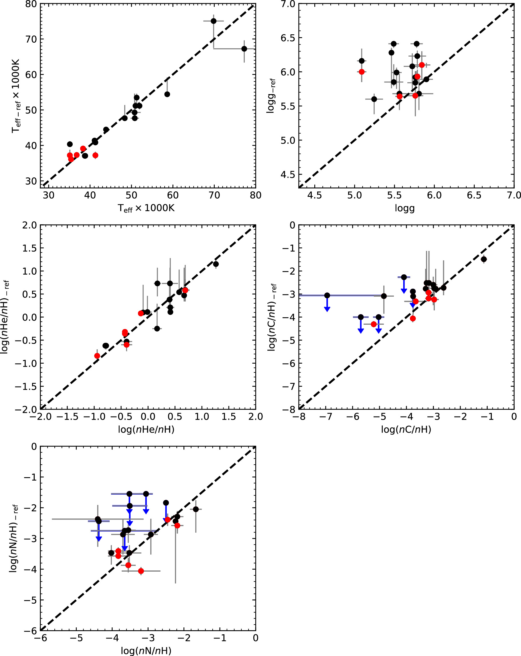
Figure 5. Comparisons of atmospheric parameters between this study and results from high- and low-resolution spectra. The red dots represent parameters obtained from high-resolution spectra (J092440.10+305013.1 and J160131.27+044027.0, Naslim et al. 2020; J091251.66+272031.4, Wild & Jeffery 2018; J113726.37+141014.1, Latour et al. 2019, Dorsch et al. 2020; and J132335.26+360759.5, Dorsch et al. 2019). Black dots denote the sample observed by Németh et al. (2012). Objects where only an upper limit is available are marked by a blue arrow pointing down.
Download figure:
Standard image High-resolution imageTable 3. Atmospheric Parameters, Galactic Velocities, and Orbital Parameters for 210 He-rich Hot Subdwarf Stars Observed in Gaia DR3 and LAMOST DR7
| No. | Label | Explanations |
|---|---|---|
| 1 | LAMOST | LAMOST target |
| 2 | RAdeg | Barycentric R.A. (J2000) a |
| 3 | DEdeg | Barycentric decl. (J2000) a |
| 4 | Teff | Stellar effective temperature |
| 5 | e_Teff | Standard error in Teff |
| 6 |

| Stellar surface gravity |
| 7 |

| Standard error of stellar surface gravity |
| 8 |

| Stellar surface He abundance |
| 9 |

| Standard error in 
|
| 10 |

| Stellar surface C abundance |
| 11 |

| Standard error in 
|
| 12 |

| Stellar surface N abundance |
| 13 |

| Standard error in 
|
| 14 |

| Logarithmic mass fraction of surface He abundance b |
| 15 |

| Standard error in 
|
| 16 |

| Logarithmic mass fraction of surface C abundance b |
| 17 |

| Standard error in 
|
| 18 |

| Logarithmic mass fraction of surface N abundance b |
| 19 |

| Standard error in 
|
| 20 | vsini | Projected rotational velocity, 
|
| 21 | e_vsini | Standard error in 
|
| 22 | pmRA | Gaia EDR3 proper motion in R.A. |
| 23 | e_pmRA | Standard error in pmRA |
| 24 | pmDE | Gaia EDR3 proper motion in decl. |
| 25 | e_pmDE | Standard error in pmDE |
| 26 | D | Gaia EDR3 stellar distance |
| 27 | e_D | Standard error in stellar distance |
| 28 | RVel | Radial velocity from LAMOST spectra |
| 29 | e_RVel | Standard error in radial velocity |
| 30 | U | Galactic radial velocity positive toward Galactic center |
| 31 | e_U | Standard error in U |
| 32 | V | Galactic rotational velocity along Galactic rotation |
| 33 | e_V | Standard error in V |
| 34 | W | Galactic velocity toward north Galactic pole |
| 35 | e_W | Standard error in W |
| 36 | Rap | Apocenter radius c |
| 37 | e_Rap | Standard error in Rap |
| 38 | Rperi | Pericenter radius c |
| 39 | e_Rperi | Standard error in Rperi |
| 40 |

| Maximum vertical height c |
| 41 |

| Standard error in 
|
| 42 | e | Eccentricity c |
| 43 | e_e | Standard error in e |
| 44 | Jz | Z-component of angular momentum c |
| 45 | e_Jz | Standard error in Jz |
| 46 | Pops | Population classification d |
| 47 | PTH | Probability in thin disk |
| 48 | PTK | Probability in thick disk |
| 49 | PH | Probability in halo |
Notes.
a At epoch 2000.0 (ICRS). b c
Form the numerical orbit integration.
d
H = halo; TK = thick disk; TH = thin disk.
c
Form the numerical orbit integration.
d
H = halo; TK = thick disk; TH = thin disk.
Only a portion of this table is shown here to demonstrate its form and content. A machine-readable version of the full table is available.
Download table as: DataTypeset image
We performed a comparative analysis of the atmospheric parameters for 15 stars within our sample, comparing them with those reported in a low-resolution spectroscopic survey of hot subluminous stars in the Galaxy Evolution Explorer survey (Németh et al. 2012). The comparisons of atmospheric parameters are presented in Figure 5, where objects indicating upper limits are denoted by blue arrows pointing downward. The average systematic shits are 700 ± 3554 K, −0.39 ±0.34 K, −0.00 ± 0.44 K, −0.46 ± 0.55 K, and −0.40 ±0.71 K for Teff,  ,
,  ,
,  , and
, and  , respectively. The comparisons indicate that Teff and
  align consistently with the current parameters. However, the systematic shifts in
  ,
,  , and
, and  are attributed to the different coverage and spectral resolution of the observations and the inclusion of rotational broadening of line profiles during the LAMOST spectral analysis. Moreover, among the six stars with available upper limits for
  and
and  , a larger dispersion was noted compared to other objects. Nonetheless, both
  and
and  for the entire sample agree with our results.
Projected rotational velocities ( ) were also determined from the LAMOST spectral analysis, and the corresponding
  values are detailed in Table 3. Among our sample, more than half (134 out of 210 spectra) exhibit consistency with no measurable
  . The subset of most extreme "rotators" (16 out of 210 spectra) comprises highly unusual cases such as misclassified WDs, cataclysmic variables, potential close binaries, and similar outliers.
In LAMOST LRS spectroscopy, individual observations are coadded, introducing orbital smearing as additional line broadening in the final spectra for binaries. Therefore, our  values serve as indicators of such extra broadening in spectral lines. This may encompass various factors like orbital smearing, inconsistencies in instrumental broadening, turbulent broadening, Stark line broadening, etc., extending beyond the actual projected rotation.
3.2. Galactic Population Classifications
We used Gaia DR3 for proper motions and distances and utilized LAMOST spectra for radial velocities to obtain the space velocity components and Galactic orbit parameters. To compute the three space velocity components U, V, and W, corresponding to the directions of the Galactic center, Galactic rotation, and north Galactic pole, respectively, we employed the software package Astropy. The parameters within Astropy were configured to set the distance from the Sun to the Galactic center at 8.4 kpc, the Cartesian velocity of the Sun in the Galactocentric frame as (11.1, 12.24, 7.25) km s−1, and the velocity of the local standard of rest (LSR) at 242 km s−1 (Schönrich et al. 2010; Irrgang et al. 2013).
We utilized the Galpy Python package to compute the Galactic orbits. Our calculations were based on the Milky Way potential model "MWpotential2014," encompassing a power-law bulge with an exponential cutoff, an exponential disk, and power-law halo components (Bovy 2015). Similar to the calculation of Galactic UVW velocities mentioned earlier, we employed the Galactocentric distance of the Sun as 8.4 kpc and the LSR velocity of 242 km s−1 (Irrgang et al. 2013). The orbit integration spanned from 0 to 3.5 Gyr in steps of 1 Myr. Extracting the Galactic orbital parameters of He-rich hot subdwarfs involved determining their apocenter (Rap), pericenter (Rperi), eccentricity (e), maximum vertical amplitude ( ), and z-component of the angular momentum (Jz
) from the integration of their orbital paths, where Rap and Rperi respectively indicate the maximum and minimum distances of an orbit from the Galactic center. The eccentricity was defined as
), and z-component of the angular momentum (Jz
) from the integration of their orbital paths, where Rap and Rperi respectively indicate the maximum and minimum distances of an orbit from the Galactic center. The eccentricity was defined as

The space velocity components and the orbital parameters can be found in Table 3. The uncertainties associated with these parameters were estimated using the Monte Carlo method. We generated 1000 random input values per star, following a Gaussian distribution. Subsequently, the output parameters and their errors were computed. Additional details on the calculation of parameter errors can be found in Luo et al. (2019).
To determine the Galactic population memberships of He-rich hot subdwarf stars, we followed the classification scheme outlined in Martin et al. (2017). This scheme builds upon the one proposed by Pauli et al. (2003, 2006) with a minor adjustment. Martin et al. (2017) introduced a slight modification by introducing the vertical scale height, setting it at Z ∼ 1.5 kpc for thick-disk stars as the cutoff height of the thin disk (Ma et al. 2017).
Our primary method for distinguishing the populations of He-rich hot subdwarf stars involved utilizing the U − V diagram, the Jz
− e diagram, and the maximum vertical amplitude  . To ensure accurate population assignments, all orbits were visually inspected to complement the automated classifications. The U − V and Jz
− e diagrams can be observed in Figure 6. Following the approach in Martin et al. (2017), we established the 3σ limits for thin-disk and thick-disk WDs (Pauli et al. 2006) in the U − V diagram using two dotted ellipses. Furthermore, we separated the positions of the thin-disk, thick-disk, and halo populations in the Jz
− e diagram using three distinct regions, referred to as regions A, B, and C, respectively.
. To ensure accurate population assignments, all orbits were visually inspected to complement the automated classifications. The U − V and Jz
− e diagrams can be observed in Figure 6. Following the approach in Martin et al. (2017), we established the 3σ limits for thin-disk and thick-disk WDs (Pauli et al. 2006) in the U − V diagram using two dotted ellipses. Furthermore, we separated the positions of the thin-disk, thick-disk, and halo populations in the Jz
− e diagram using three distinct regions, referred to as regions A, B, and C, respectively.

Figure 6. Kinematic properties. Top panel: U − V velocity diagram. The two dashed ellipses denote the 3σ limits for the thin-disk and thick-disk populations from Pauli et al. (2006), respectively. The cyan star represents the LSR. Bottom panel: Z-component of the angular momentum (Jz ) vs. eccentricity (e). The two parallelograms represent the regions of the thin disk and thick disk (Pauli et al. 2006).
Download figure:
Standard image High-resolution imageAs detailed in Luo et al. (2020, 2021), thin-disk stars are identified within the 3σ thin-disk contour in the U − V diagram and fall within region A in the Jz
− e diagram. Their orbits exhibit minor excursions in Galactocentric distance (R) and from the Galactic plane in the Z-direction, typically confined in the range of  . Thick-disk stars are situated within the 3σ thick-disk contour and in region B. These stars display greater orbit extension in both R and Z compared to thin-disk stars but less than that of halo stars. Halo stars reside outside regions A and B, as well as beyond the 3σ thick-disk contour. Their orbits show substantial differences in R and Z, with some halos exhibiting an extension in Galactocentric distance (R) larger than 18 kpc or a vertical distance from the Galactic plane (Z) larger than 6 kpc.
4. Results and Discussions
4.1. Helium Abundance versus Effective Temperature
Figure 7 displays the distributions of 210 program stars in the  panel, representing the thin-disk, thick-disk, and halo populations. Based on our helium classification scheme (see Luo et al. 2021), 191 stars are identified as He-rich hot subdwarf stars. Among these He-rich hot subdwarf stars, 127 were further categorized as eHe, while 64 were classified as iHe with
  .
.

Figure 7. Helium abundances vs. effective temperature. Two gray ellipses represent the iHe groups defined by Luo et al. (2021).
Download figure:
Standard image High-resolution imageFigure 7 reveals a trend showing a gradual decrease in helium abundance with increasing temperature, notably observed among the eHe stars. This pattern appears to persist across the thin-disk, thick-disk, and halo populations. Interestingly, we did not identify the two distinct eHe subclasses previously reported by Luo et al. (2021). However, notable distinctions in the effective temperature distribution for the eHe stars in the halo population were observed when compared to those in the thin and thick disks. Particularly, eHe stars in the halo exhibit a distinct gap near Teff = 46,000 K in the  panel. The number ratio of eHe stars with Teff > 46,000 K to those with Teff < 46,000 K is 16:6 for the halo population, 26:26 for the thick-disk population, and 21:31 for the thin-disk population. This observation does not explicitly support the existence of two distinct subclasses of eHe stars, especially in the thin-disk and thick-disk populations. However, the number ratio of eHe stars with Teff > 46,000 K to those with Teff < 46,000 K appears to gradually increase from the thin to the thick disk and further to the halo populations, using Teff = 46,000 K as the classification criterion, as previously outlined by Luo et al. (2021).
Figure 7 shows the presence of two separate iHe groups, as previously identified by Luo et al. (2021). These groups are represented by gray ellipses in the figure. According to the findings of Luo et al. (2021), group iHe-1 exhibits a notably distinct Galactic population fraction in comparison to group iHe-2. Specifically, the former presents a thin-disk population fraction of 63% ± 9%, while the latter demonstrates a thin-disk population fraction of 80% ± 13%.
4.2. Carbon and Nitrogen Abundances versus Helium Abundance
Figure 8 displays the distributions of He-rich hot subdwarf stars in both the  and
and  panels. These trends are represented by dashed lines in the top panel for C abundances and in the bottom panel for N abundances, as shown in Figure 7. Our sample exhibits similar patterns of C and N as reported in Németh et al. (2012), demonstrating a distinct trend with higher average C and N concentrations at higher He abundances. In Figure 8, two best-fitting trends are plotted for C abundances using dashed lines in the top panel,
and for N abundances in the bottom panel,
respectively. These two trends are taken from Németh et al. (2012).
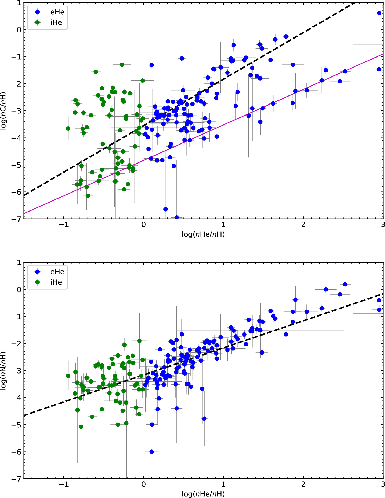
Figure 8. Abundance correlations. Top panel:  diagram. Bottom panel:
  diagram. The dashed lines represent the best-fit trends published by Németh et al. (2012).
Download figure:
Standard image High-resolution imageIn the top panel of Figure 8, two probable C–He sequences are observed for eHe hot subdwarf stars. Approximately two-thirds of these stars align within the first C–He sequence, consistent with the current best-fit trend. The second C–He sequence consists of eHe hot subdwarfs characterized by low carbon abundances. This suggests that eHe hot subdwarf stars belonging to these two C–He sequences likely stem from entirely distinct formation channels. Likewise, among iHe hot subdwarf stars, we also observe two different C groups. Those within the high C group do not align with the first C–He sequence of eHe hot subdwarf stars, indicating that the origin of high carbon stars in both the eHe and iHe subtypes might lack an evolutionary correlation.
The high carbon group of iHe hot subdwarf stars does not align with the first C–He sequence observed in eHe hot subdwarf stars, suggesting a lack of correlation in the evolutionary origins of high C stars between the eHe and iHe subtypes. However, iHe hot subdwarf stars in the low C group show a good agreement with the second C–He sequence of eHe hot subdwarf stars, implying a potential inherent correlation between low C stars in both the eHe and iHe groups regarding their origins. Nevertheless, it was observed that iHe hot subdwarf stars in the low C group align well with the second C–He sequence of eHe hot subdwarf stars, suggesting that stars exhibiting low C abundance in both the eHe and iHe subtypes may share an inherent correlation in their origins.
The bottom panel of Figure 8 shows that both eHe and iHe hot subdwarf stars do not exhibit clear differences in the N–He distribution. Most of these stars appear to follow a N–He sequence that aligns well with the best-fit trend identified by Németh et al. (2012).
4.3. Determined Abundances versus Effective Temperature
For a statistical comparison with the SPY sample of Hirsch (2009), the determined abundances are defined by mass fraction:  , where i represents He, C, and N. Figure 9 shows the distributions of He-rich hot subdwarf stars in the
  ,
,  , and
, and  panels. In Figure 9, the SPY sample from Hirsch (2009) is denoted by magenta dots. Moreover, Schindewolf et al. (2018) conducted an analysis of high-resolution visual and ultraviolet spectra of four He-rich sdO stars. These four stars are marked in Figure 9 with red dots. Our findings show that both the SPY sample and the four He-rich sdO stars studied by Schindewolf et al. (2018) fall within the range of our sample in both the
  and
and  diagrams.

Figure 9. Determined abundances in logarithmic mass fractions vs. effective temperatures. Top panel: He abundances. Middle panel: C abundances. Bottom panel: N abundances. The black horizontal dashed lines represent the solar values. The magenta dashed line is  . The magenta dots denote the sample of He-rich hot subdwarf stars given by Hirsch (2009), and the red dots represent the four He-rich sdO stars observed by Schindewolf et al. (2018).
Download figure:
Standard image High-resolution imageIn the  panel, our sample exhibits a distinctly bimodal distribution of C abundances, aligning with the observations of Hirsch (2009). This distribution can be categorized into two primary groups: the C-enriched and C-deficient groups, distinguished at
  . The C-enriched subgroup further divides into C-enriched eHe and C-enriched stars at Teff = 43,000 K. Meanwhile, the carbon-deficient group comprises a mixture of eHe and iHe hot subdwarf stars. Consequently, three distinct groups exist in the
  panel. The first group comprises C-enriched eHe hot subdwarf stars, showing a trend where C abundances decrease from supersolar values to below the solar value as the effective temperature increases. Specifically, for Teff > 47,000 K, the first group demonstrates C abundances below the solar value. In contrast, for Teff < 47,000 K, this group presents C abundances above the solar value. Notably, this region encompasses nearly all the stars from both the SPY sample by Hirsch (2009) and the sample by Schindewolf et al. (2018). The second group predominantly includes C-enriched iHe hot subdwarf stars spanning a wide temperature range from 16,000 to 40,000 K. Our sample indicates that the third group aligns with the findings of Hirsch (2009). This group comprises a mix of eHe and iHe stars with approximately half of the iHe stars falling into this category. The distributions of these stars suggest that eHe and iHe stars within this third group likely share similar formation pathways.
In the  diagram, there is no clear division observed in the N abundances. More than 82% of the He-rich stars exhibit N abundances surpassing the solar value, which is proportionally higher than the two-thirds value found in the SPY sample by Hirsch (2009). Notably, all four He-rich sdO stars studied by Schindewolf et al. (2018) also show N abundances above the solar value. Moreover, a discernible pattern is observed where N appears to be more abundant in objects with a lower C content compared to those with higher C abundances. It was also observed that the average N abundance decreased with increasing temperatures in eHe stars, in line with the findings of Hirsch (2009).
Figure 10 presents the distributions of C and N abundances within the Galactic thin-disk, thick-disk, and halo populations, aimed at unveiling insights into He-rich hot subdwarfs with distinct C subclasses based on kinematics. A notable observation is the bimodal distribution of C abundance evident in both eHe and iHe hot subdwarf stars within the thin- and thick-disk populations, while C-deficient stars are notably scarce in the halo population. The proportion of C-enriched eHe and iHe stars progressively increases from the thin-disk to the halo population, in contrast to carbon-deficient stars. The stark absence of C-deficient stars within the halo population suggests that C-enriched and C-deficient stars have different origins. Regarding the N abundance distributions, no significant differences are observed between eHe and iHe stars across the thin-disk, thick-disk, and halo populations.

Figure 10. Determined C and N abundances in logarithmic mass fractions vs. effective temperatures in the Galactic halo, thick-disk, and thin-disk populations, respectively.
Download figure:
Standard image High-resolution image
4.4. Discussions
In our prior investigation (Luo et al. 2021), we categorized eHe hot subdwarf stars into two groups, labeled eHe-1 and eHe-2, within the  panel. The classification criterion set at Teff = 46,000 K allowed for this distinction. Our galactic population analysis revealed a higher prevalence of the eHe-2 group within the thin-disk population compared to the eHe-1 group. However, in our present study, we were unable to discern the two distinct eHe subclasses reported by Luo et al. (2021). Instead, our sample exhibits a continuous trend displaying a decreasing He abundance with increasing temperature. While this consistent trend of decreasing helium abundance with temperature persisted across the thin-disk, thick-disk, and halo populations, an observable gap emerged among eHe stars in the halo population near Teff = 46,000 K within the
  panel. Although our data did not support the existence of the two distinct subclasses of eHe stars described by Luo et al. (2021), particularly within the thin- and thick-disk populations, we did note a gradual increase in the ratio of eHe stars with Teff > 46,000 K to those with Teff < 46,000 K. This trend was consistent from the thin disk to the thick disk and then to the halo populations, aligning with the findings of Luo et al. (2021). Moreover, our observations indicated that C-deficient stars were primarily located at Teff < 46,000 K, and their prevalence decreased gradually from the thin disk to the thick disk and halo populations. These results suggest that the presence of C-deficient stars could impact the distribution of eHe stars within the various Galactic populations.
The merger of double HeWDs is considered a key scenario in explaining the formation of isolated He-rich hot subdwarf stars (Han et al. 2002). Zhang & Jeffery (2012) proposed three merger models of double HeWDs: slow accretion from debris, fast accretion from a corona, and a combination of both processes. Their findings suggested that fast hot mergers result in C-rich, N-poor surfaces; slow cold mergers lead to N-rich surfaces; and composite models yield C- and N-rich surfaces. Yu et al. (2021) demonstrated that the merger of double HeWDs can account for the bimodal distribution of C abundances, where the C-enriched eHe stars are formed by high-mass HeWDs and the C-deficient ones by low-mass HeWDs. This finding aligns with the observations of eHe hot subdwarf stars in the Galactic field (Luo et al. 2019), supporting the predictions stemming from the double HeWD merger scenario. The fraction of C-enriched eHe hot subdwarf stars exhibits a consistent, monotonic increase from the thin disk to the halo population, aligning with the predictions from the merger models of double HeWDs (Yu et al. 2021). However, the distribution of C-deficient eHe hot subdwarf stars demonstrates an opposite tendency, inconsistent with the expected outcome from double HeWD merger models. Moreover, Hirsch (2009) observed different behaviors in the rotational velocities of C-enriched and C-deficient eHe hot subdwarf stars. The former displayed significantly higher projected rotational velocity compared to the latter, providing further support for the double HeWD merger channel in the formation of C-enriched eHe hot subdwarf stars.
The late hot flasher scenario (Miller Bertolami et al. 2008) provides a potential explanation for He-rich hot subdwarf stars. According to Luo et al. (2021), the evolutionary tracks within this scenario can align with eHe stars having Teff < 46,000 K and iHe stars in the  diagram. However, upon detailed comparisons with the findings of Hirsch (2009), it was concluded that the late hot flasher scenario does not account for the presence of C-deficient He-rich hot subdwarf stars. Additionally, Battich et al. (2018) conducted calculations of surface abundances for various late hot flasher scenarios, incorporating updated electron-conduction opacities introduced by Cassisi et al. (2007). Their results indicated a qualitative agreement of surface abundances with those proposed by Miller Bertolami et al. (2008). Despite this, further investigation is required to elucidate the formation channel of C-deficient He-rich hot subdwarf stars.
5. Conclusions
Using the LAMOST DR7 spectra, we conducted an analysis of the H, He, C, and N abundances of 210 He-rich hot subdwarf stars collected from various literature references, confirming 191 stars as He-rich hot subdwarf stars. Following our established He classification scheme described in Luo et al. (2021), our examination identified 127 He-rich stars as eHe and 64 as iHe stars. The analysis of the sample revealed two C sequences within the  plane and one N sequence within the
  plane. The observed C-enriched sequence and the N sequence closely correspond to the findings of Németh et al. (2012). However, the C-deficient sequence observed in our sample was not present in the data of Németh et al. (2012). While the C sequence trend published by Németh et al. (2012) aligns with C-enriched eHe stars, it appears unsuitable for iHe hot subdwarf stars. This suggests that C-enriched eHe and iHe stars may have different formation pathways. Moreover, our discovery of a C-deficient sequence suggests a probable evolutionary connection between C-deficient eHe and iHe stars.
In the  plane, He-rich hot subdwarf stars present a clear dichotomy concerning the C abundance, allowing for their categorization into C-enriched and C-deficient groups. By combing the He and C abundances, we have identified three distinct groups within the
  plane. C-enriched stars are further split into C-enriched eHe and C-enriched iHe groups, while the third group comprises primarily C-deficient eHe and iHe stars. Notably, N enrichment beyond solar levels is observed in approximately 82% of our targets, showing a trend where the average N abundances of eHe stars decrease with increasing effective temperatures.
The combined data of radial velocities from LAMOST and the parallaxes and proper motions from Gaia DR3 were utilized to determine the Galactic population memberships of He-rich hot subdwarf stars. Our findings indicate that a bimodal distribution of C abundance is present within the thin and thick disks but notably absent in the halo population. Particularly, the lack of C-deficient stars within the halo was observed. The origin of C-deficient He-rich hot subdwarf stars remains a mystery, as neither the merger of double HeWDs nor the late hot flasher scenario appears capable of explaining their existence.
Acknowledgments
This work is supported by the National Key R&D Program of China (Nos. 2021YFA1600401 and 2021YFA1600400), the National Natural Science Foundation of China (NSFC) under grant 12173028, the Chinese Space Station Telescope project (CMS-CSST-2021-A10), the Sichuan Youth Science and Technology Innovation Research Team (grant No. 21CXTD0038), and the Innovation Team Funds of China West Normal (No. KCXTD2022-6). P.N. acknowledges support from the Grant Agency of the Czech Republic (GAČR 22-34467S). The Astronomical Institute in Ondřejov is supported by the project RVO:67985815. Guoshoujing Telescope (the Large Sky Area Multi-Object Fiber Spectroscopic Telescope, LAMOST) is a National Major Scientific Project built by the Chinese Academy of Sciences. Funding for the project has been provided by the National Development and Reform Commission. LAMOST is operated and managed by the National Astronomical Observatories, Chinese Academy of Sciences. This work has made use of data from the European Space Agency (ESA) mission Gaia (https://www.cosmos.esa.int/gaia), processed by the Gaia Data Processing and Analysis Consortium (DPAC; https://www.cosmos.esa.int/web/gaia/dpac/consortium). Funding for the DPAC has been provided by national institutions, in particular, the institutions participating in the Gaia Multilateral Agreement. This research has used the services of www.astroserver.org under reference PF2EFZ.
Facilities: LAMOST - , Gaia -
Software: astropy (Astropy Collaboration et al. 2013, 2018), galpy (Bovy 2015).