


Abstract
The Tianwen-1 (TW1) Mars probe experienced solar conjunction for the first time in 2021. The China VLBI Network (CVN) observes the differential one-way ranging (DOR) signals of TW1 throughout its phase. This paper explores the application of CVN observation data to study the solar wind plasma. First, the frequency and phase of the DOR carrier and sidetones at each station are calculated using the Doppler method. Then, the variations in both the differential phase delays (DPD) and the total electron content (TEC) are calculated using the phase of the sidetones. We also statistically analyze the fluctuations in the Delta-DOR (ΔDOR) group delay. The results indicate that the fluctuations of the frequency, phase, ΔDOR group delay, delay rate, and TEC variations of the TW1 signals increase with the decrease of the heliocentric distance. On 2021 November 2, a coronal mass ejection (CME) passed across the ray paths of the telescope beams, when the heliocentric distance and heliographic latitude of the projected position of Mars were 30.6 Rs and 3°, respectively. Our data catch the impact of the CME on the DOR signals. The change of the DPD reaches 170 ps, which is equivalent to 986 TECU. We utilize the cross correlation to analyze the frequency fluctuations at multiple stations, and obtain the propagation direction and velocity variations of the CME. Our analysis indicates that multifrequency DOR signals observed by very long baseline interferometry stations have great application to characterize the electron density variations and propagation of the solar wind plasma.
Export citation and abstract BibTeX RIS

Original content from this work may be used under the terms of the Creative Commons Attribution 4.0 licence. Any further distribution of this work must maintain attribution to the author(s) and the title of the work, journal citation and DOI.
1. Introduction
Exploring the properties of solar wind has captivated the interest of many space physics researchers. There are more scientific ways to study solar wind plasma than ever before, such as the use of very long baseline interferometry (VLBI) technology to propose a coronal electron density model for radio-source observations near the Sun (Soja et al. 2014), the use of short-baseline interference techniques to obtain coronal electron density (Muhleman et al. 1970), the use of spacecraft radio-sounding experiments to characterize the interplanetary phase scintillation (Molera Calvés et al. 2014), and the combination of various solar probe data resources such as the Parker Solar Probe to achieve real-time space weather forecasting of coronal mass ejection (CME) activities (Palmerio et al. 2022).
Since the radio signals of spacecraft can enter the challenging inner solar wind within 10 solar radii (Rs, 1 Rs = 695,700 km), solar conjunction observation of deep-space probes is a common research method to study the coronal structure. This technique was used by Akatsuki to show the difference in the solar-wind velocity between fast and slow winds (Chiba et al. 2022), by Galileo to study the outer turbulence scale of the solar wind (Efimov et al. 2002), by Venus Express to detect the strong turbulence regions in the super corona (Efimov et al. 2021), by Mars Express to study the interplanetary plasma scintillation between the years 2013–2020 (Molera Calvés et al. 2017; Kummamuru et al. 2023), by the Mercury Surface, Space Environment, Geochemistry, and Ranging spacecraft to study radio Faraday rotation through a CME (Jensen et al. 2018), and in Tianwen-1 (TW1) to detect the oscillation and propagation of the nascent dynamic solar wind structure (Ma et al. 2022).
TW1 is the first Chinese probe to be successfully launched and landed on Mars. TW1 consists of an orbiter and a rover. It was launched on 2020 July 23 and arrived on Mars on 2021 February 10. On 2021 May 15, following the separation of the orbiter and the rover, the rover successfully landed softly on Mars while the orbiter continued to fly around the planet (Zhang et al. 2022). The Chinese VLBI network (CVN), consisting of the Shanghai (SH) 25 m, Beijing (BJ) 50 m, Kunming (KM) 40 m, Urumqi (UR) 26 m, and Tianma (TM) 65 m stations, and the Shanghai VLBI Data Processing Center (VLBI center), participates in the orbit determination of TW1 by performing Delta–differential one-way ranging (ΔDOR) observation (James et al. 2009; Liu et al. 2022).
In this study, we utilize the TW1 differential one-way ranging (DOR) signals of the orbiter observed by VLBI radio telescopes to study their application in solar wind plasma and CMEs. We analyze the statistical fluctuations of the frequency, phase, ΔDOR group delay, delay rate, and total electron content (TEC) variations at different heliocentric distances of the TW1 signals. Furthermore, we estimate the propagation velocity and direction of a CME on 2021 November 2. Section 2 presents the methodology of the research. Section 3 shows the statistical analysis of the fluctuations of ΔDOR delay, delay rate, frequency, phase, and TEC variations. Section 4 verifies the CME on 2021 November 2 and measures its velocity by cross correlation analysis of the frequency scintillation. Section 5 presents the conclusion.
2. Methodology
2.1. Observation
The DOR signals transmitted by TW1 consist of multiple single-frequency signals. After 2020 July 26, the x-band DOR signals are transmitted by a 2.5 m high-gain directional antenna instead of the low-gain omnidirectional antenna (Sun et al. 2021; Liu et al. 2022). Figure 1 shows the distribution of the DOR signals that consist of the carrier frequency and two groups of sidetones. The maximal frequency span between the sidetones is 38.4 MHz (CCSDS 2019).
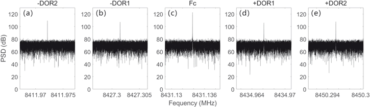
Figure 1. Power density spectra of Tianwen-1 (TW1) at BJ station at 02:15 on 2021 November 12. Fc is the carrier frequency at 8431 MHz. (a) −DOR2 = Fc − 19.2 MHz, (b) −DOR1 = Fc − 3.8 MHz, (c) Fc = 8431 MHz, (d) +DOR1 = Fc + 3.8 MHz, (e) +DOR2 = Fc + 19.2 MHz.
Download figure:
Standard image High-resolution imageFurthermore, the signals of the TW1 are divided into two modes, coherent and incoherent signals. In the coherent mode, the transponder on board receives the uplink signals generated by a high stability ground-based hydrogen clock, then retransmits them to the Earth. In contrast, the downlink signals generated by the onboard crystal oscillator is the incoherent signals. The stability of the ground hydrogen clock is 10−15 s s−1, superior to the onboard crystal oscillator of 10−12 s s−1 (Ma et al. 2022; Wang et al. 2022).
In ΔDOR observations, the radio telescopes of the CVN stations observe the extragalactic radio source and spacecraft alternately (detector–radio source–detector) (James et al. 2009; CCSDS 2019; Shu et al. 2017; Liu et al. 2022). The purpose of observing the radio source is to correct the common errors in ΔDOR group delay from internal instruments and the Earth's ionosphere and atmosphere. So far, CVN has conducted more than 200 observations of TW1. During the first solar conjunction observation of TW1, we select 10 days of data as symmetrically as possible according to the variations of heliocentric distance around the solar conjunction (Table 1). Every observation consists of 8–27 scans, and the duration of each scan is 3–10 minutes. The interval between scans is 7 min. The heliocentric distance of the selected data range from 129.4 to 33.5 Rs is in the ingress phase, and 13.5–102.1 Rs is in the egress phase. It should be noted that TW1 switched off the downlinked DOR signals and entered into safe mode during the solar conjunction phase from 2021 September 15 to October 18. Therefore, the CVN did not carry out the ΔDOR observation during this period. In addition, time throughout the paper is in coordinated universal time (UTC).
Table 1. Specifications of the Observations: Date, Time, Stations, Calibrator Source, Heliocentric Distances, Number of Scans, Coherent or Incoherent, Ingress or Egress
| Date | Time | Station | Extragalactic Radio Source | Heliocentric Distance (Rs) | No. of Scans | Coherent/Incoherent | Ingress/Egress |
|---|---|---|---|---|---|---|---|
| 2021.06.18 | 04:30–09:10 | SH;BJ;UR;TM | 0748+126 | 129.4 | 15 | Co+Inco | I |
| 2021.08.20 | 03:00–07:10 | SH;KM;UR | 1038+064 | 59.9 | 14 | Inco | I |
| 2021.09.11 | 01:10–08:50 | SH;BJ;UR | 1219+044 | 33.5 | 27 | Co+Inco | I |
| 2021.10.19 | 02:30–08:10 | SH;KM;UR | 1334–127 | 13.5 | 19 | Co+Inco | E |
| 2021.10.20 | 01:00–08:10 | SH;UR | 1334–127 | 14.8 | 25 | Co+Inco | E |
| 2021.10.26 | 04:10–08:10 | SH;KM;UR | 1334–127 | 22.1 | 13 | Inco | E |
| 2021.11.02 | 01:10–05:40 | SH;BJ;KM;UR | 1406–076 | 30.6 | 15 | Co | E |
| 2021.11.09 | 01:00–07:30 | SH;BJ;UR | 1406–076 | 39.1 | 22 | Co+Inco | E |
| 2021.11.21 | 04:00–06:40 | SH;KM;UR | 1511–100 | 53.4 | 8 | Inco | E |
| 2022.01.04 | 03:00–07:10 | SH;BJ;UR | 1622–253 | 102.1 | 10 | Co+Inco | E |
Download table as: ASCIITypeset image
2.2. Data Processing
Figure 2 represents the differential VLBI observation and data-processing flow chart by CVN. The radio frequency signals received by each CVN station are converted into baseband signals and recorded by the Chinese VLBI Data Acquisition System terminal (Zhu et al. 2021). The record format is as follows: four channels, 8 MHz bandwidth, 16 MHz sampling rate, and 2-bit quantization. The raw observation data are transferred to the VLBI center for processing. The solid box represents the existing VLBI correlator process to obtain the ΔDOR group delay and delay rate used for the orbit and position determination of the spacecraft (Zheng et al. 2020). In this paper, we mainly focus on the Doppler process to study the application of DOR signals in solar plasma. The third-order phase locked loop (PLL) is used to obtain the frequency and phase of DOR signals (Deng et al. 2021). Then the frequency and phase used to calculate the solar wind velocity, DPD, and TEC variations.
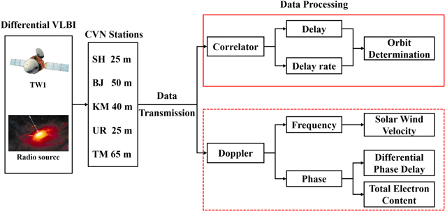
Figure 2. Flow chart of the data processing.
Download figure:
Standard image High-resolution imageThe sampling time of the frequency and phase of the PLL output is 0.01 s. It takes a few seconds for the PLL algorithm to start relocking from unlocking. Hence, we actively delete the first 10 s of data as it contains invalid information in each scan. In addition, when the working mode of the onboard transponder is switched, a sudden change in the transmitting frequency of the probe will cause the PLL to unlock. We delete these scans containing transponder mode switching.
After obtaining the phases and frequencies of DOR sidetones, we calculate the DPD as
where Δτ12 is the DPD, and f1 and f2 are the lowest and highest frequencies of DOR sidetones, respectively. ϕ1 and ϕ2 are the corresponding phases. The influences from the orbit, the Earth's atmosphere, and ground instruments can be removed. Therefore, large DPD variations are proportional to TEC changes in the ray path (Bird 1982; He et al. 2022)
where D is the TEC variations and c is the light speed. Equation (2) demonstrates that the DPD is inversely proportional to the change in TEC. It is important to note that the absolute value of the TEC within a single scan cannot be calculated due to the cycle ambiguities between scans, but only the relative variations of the TEC (Bird 1982). In practice, simultaneously applying dual-band radio ranging measurements with the Doppler measurements can eliminate the ambiguity (Jensen et al. 2016, 2018). However, due to the absence of range data, we can only study relative TEC values.
To analyze the effect of the solar plasma on DOR signals, we first perform a 1 s integral on the data in the time domain. Second, a seventh-order polynomial fit is applied to the frequency or phase time series to determine the tendency of variations, then it is subtracted from the time series to generate the frequency and phase fluctuation time series about zero. The standard deviations (STDs) of the fluctuations are obtained. Third, according to the signals mode, the data are divided into coherent and incoherent scans. We average the STDs of scans for each mode. Finally, the STDs of all observation stations are averaged to obtain the final results.
To study the change of TEC with different heliocentric distances, we calculate the STDs of the D directly using TEC data with an integration time of 1 s without fitting. Data are then classified again into two categories: coherent and incoherent. We also average the STDs of scans with the same mode and then average the STDs across all observation stations.
To study the effect on ΔDOR group delay and the delay rate from solar wind plasma, we first perform quadratic polynomial fitting on the delay data of the probe with an integration time of 30 s for each scan of each baseline. Then, we calculate the STDs of the fitting residuals. Finally, the STDs of all scans from all baselines are averaged. It should be noted that during the ΔDOR group delay determination process, we utilize observational data from a calibrator source. As a result, ΔDOR group delay fluctuations are primarily influenced by plasma and also contain a minor amount of radio source phase error. Note that the heliocentric distance of the calibrator source is within the range of 10–122 Rs. When the heliocentric distance of the calibrator source decreases, it will introduce more phase errors into the ΔDOR group delay (CCSDS 2019). The impact of the calibrator source on the delay rate is subtracted during the differencing step. In addition, the phase, frequency of signals, and TEC are not affected by the calibrator source since we process only the detector's raw data with Doppler directly but without involving a calibrator source. All data-processing results are shown in Table 2.
Table 2. Statistical Analysis: ΔDOR Group Delay, Delay Rate, Frequency, Phase, and TEC
| Date | DORSTD a | RSTD b | FSTD c | PSTD d | DSTD e | |||
|---|---|---|---|---|---|---|---|---|
| (ns) | (ps s−1) | (Hz) | (rad) | (TECU) | ||||
| Coherent | Incoherent | Coherent | Incoherent | Coherent | Incoherent | |||
| 2021.06.18 | 0.021 | 0.285 | 0.009 | 0.012 | 0.376 | 1.165 | 2.157 | 2.949 |
| 2021.08.20 | 0.025 | 0.299 | ... f | 0.012 | ... | 0.975 | ... | 2.703 |
| 2021.09.11 | 0.048 | 0.453 | 0.025 | 0.017 | 1.310 | 1.008 | 6.835 | 3.564 |
| 2021.10.19 | 0.058 | 2.688 | 0.110 | 0.064 | 4.062 | 2.955 | 26.771 | 14.204 |
| 2021.10.20 | 0.055 | 1.839 | 0.149 | 0.084 | 5.521 | 2.841 | 15.256 | 22.403 |
| 2021.10.26 | 0.025 | 0.517 | ... | 0.025 | ... | 1.231 | ... | 4.008 |
| 2021.11.02 | 0.073 | 1.761 | 0.073 | ... | 2.954 | ... | 16.461 | ... |
| 2021.11.09 | 0.027 | 0.295 | 0.018 | 0.017 | 0.507 | 1.207 | 3.220 | 2.528 |
| 2021.11.21 | 0.024 | 0.293 | ... | 0.014 | ... | 0.966 | ... | 2.973 |
| 2022.01.04 | 0.023 | 0.318 | 0.008 | 0.013 | 0.351 | 1.188 | 3.296 | 1.871 |
Notes.
a DORSTD means the STDs of ΔDOR group delay fluctuations, determined after detrending the data using a quadratic polynomial fitting fit. b RSTD means the STDs of delay rate fluctuations, determined after detrending the data using a quadratic polynomial fitting fit. c FSTD means the STDs of frequency fluctuations, determined after detrending the data using a seventh-order polynomial fit. d PSTD means the STDs of phase fluctuations, determined after detrending the data using a seventh-order polynomial fit. e DSTD means the STDs of TEC variations. f ... means that there are no observation data with the corresponding mode signals.Download table as: ASCIITypeset image
3. Data Analysis
Analysis of signals characteristics at different heliocentric distances can be used to study the influence of solar wind plasma on probe signals in the complex interplanetary space environment. The observation data of all VLBI stations are calculated for further analysis. Figure 3 represents the statistical results for the STDs of the ΔDOR group delay, delay rate, frequency, and phase, respectively. With the decrease of the heliocentric distance (the signals propagation path is getting closer to the Sun), the ΔDOR group delay fluctuations increase from 0.021 to 0.058 ns. The variations of the delay rate range from 0.285 to 2.688 ps s−1. Meanwhile, the STDs of frequency and phase fluctuations increase, from 0.009 to 0.149 Hz for frequency, and 0.351 to 5.521 rad for phase. It is noted that the DORSTD increased to 0.048 ns on 2021 September 11 due to the higher noise level of SH between 03:17:00 and 04:46:00.

Figure 3. STDs of fluctuations of TW1 signals at different heliocentric distances (ingress: 129.4 Rs (2021 June 18) − 33.5 Rs (2021 September 11); egress: 13.5 Rs (2021 October 19) − 102.1 Rs (2022 January 4)). (a) ΔDOR group delay, (b) delay rate, (c) frequency, (d) phase.
Download figure:
Standard image High-resolution imageIn general, coherent signals tend to have less frequency fluctuations than incoherent signals due to their higher frequency stability. However, when the heliocentric distance drops below 39.1 Rs, the frequency fluctuations of incoherent signals are lower than coherent signals. This is because the coherent signals are affected twice in both the uplink and downlink, while only the downlink of the incoherent signals is affected by solar wind plasma. Therefore, the impact of the solar wind on the signals is greater than the frequency stability when the heliocentric distance is less than 39.1 Rs.
Besides the solar wind plasma, the probe signals are also disturbed by other factors during propagation, such as Earth's ionosphere. The orbit information of TW1 within our selected dates indicates that the minimum distance of the probe's signal path to Mars always exceeded 5000 km above the Martian ionosphere (Gurnett et al. 2008). Therefore, the probe's signal path is unaffected by it. Statistical analysis of the TEC variations of the signal's path under different heliocentric distances can directly reflect the TEC change caused by all interference factors on the ray path. It is worth noting that due to the scheduling of the overall mission's observation plan for TW1, we do not have both coherent and incoherent signal observations every day. Figure 4 shows the variations of the TEC along the line of sight at different heliocentric distances. With the decrease of heliocentric distance, the variations of TEC increase gradually from 2.0 to 26.97 TECU. We can see that the closer the ray path is to the Sun, the stronger the signal fluctuations. However, the TEC variations on 2021 November 2 suddenly increase compared to 2021 October 26. The former is 16.499 TECU with a heliocentric distance of 30.6 Rs, which is about 3 times more than 6.134 TECU on the latter at 22.1 Rs. Meanwhile, in Figure 3, the fluctuations in ΔDOR group delay, delay rate, frequency, and phase sharply increase on November 2 as well. The subsequent analysis shows that one CME event occurred on 2021 November 2. It should be noted that the heliocentric distances on both October 19 and October 20 are relatively close, around 14 Rs. The solar activity on October 20 may have more impact on the coherent signals, resulting in greater fluctuations compared to October 19 in Figures 3 and 4.
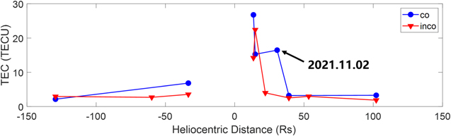
Figure 4. STDs of TEC variations at different heliocentric distances (ingress: 129.4 Rs (2021 June 18) − 33.5 Rs (2021 September 11); egress: 13.5 Rs (2021 October 19) − 102.1 Rs (2022 January 4)).
Download figure:
Standard image High-resolution imageThe variations of TEC in the coherent mode on October 19 are significantly greater than that on October 20, which appears inconsistent with the statistical results of phase and frequency. In fact, the STDs of the D represents the amplitude of TEC relative variations, while the STDs of the phase and frequency-fitting residual represents the magnitude of TEC fluctuations. We calculated the STDs of the TEC-fitting residuals on both October 19 and October 20. The trend in STDs of the TEC fluctuations aligns with the trends in frequency and phase fluctuations.
4. Coronal Mass Ejections
4.1. CME Verification
We compare the radio observation data of TW1 and the Large Angle and Spectromeric Coronagraph Experiment (LASCO) data of the Solar and Heliospheric Observatory (SOHO) to study the effects of CMEs on spacecraft signals. The changing trends of the STDs of the fluctuations of frequency, phase, and TEC variations for the four stations are consistent in Figure 5, which excludes the possibility of the anomaly on a single station. The TEC variations induced by Earth's ionosphere are calculated using global navigation satellite system data. To eliminate the influence of the ionosphere, we subtract this component from the TEC measurements (Zhou et al. 2020). It can be seen that the frequency, phase, and TEC change increases gradually after 03:00 (Figure 5). The frequency fluctuation is ±0.15 Hz before the outbreak of the CME, with a maximum up to ±1 Hz after the eruption. Meanwhile, the variations of phase fluctuations and TEC range from 5 to 71 rad, and 40 to 265 TECU, respectively. In Figure 5(c), the variation of TEC has exceeded 250 TECU between UTC 05:00 and 05:30.
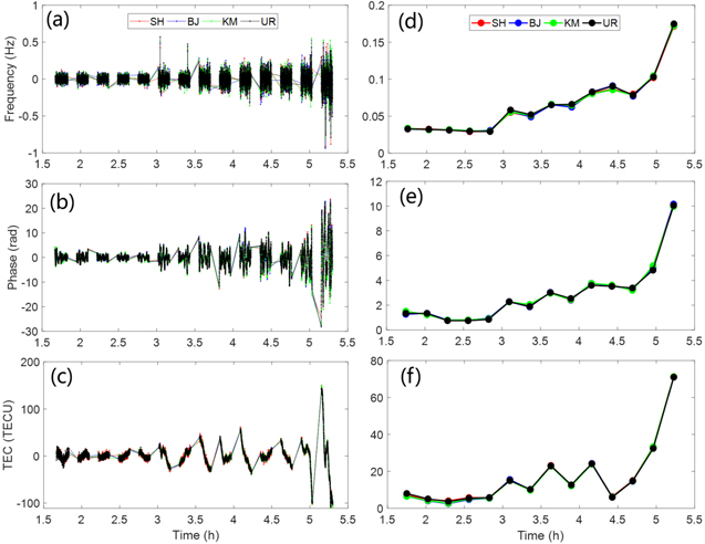
Figure 5. The fluctuations of the (a) frequency, (b) phase, and (c) TEC variations. The STDs of the fluctuations of the (d) frequency, (e) phase, and (f) TEC variations on 2021 November 2.
Download figure:
Standard image High-resolution imageFigures 6(a) and (b) show LASCO C3 images on 2021 October 26 and 2021 November 2. The position of Mars on 2021 October 26 is marked with a black arrow in Figure 6(a). Mars's position on 2021 November 2 is outside of the frame in Figure 6(b). The effective imaging range of the C3 is 32 Rs. However, the CCD detector in LASCO C3 is a square with a side length of 21 mm, and its imaging range is a square circumscribed by a circle with a radius of 30 Rs. On 2021 November 2, the apparent heliocentric distance to the line of sight to Mars is 30.6 Rs, and Mars is located in an area outside the CCD's imaging range (Brueckner et al. 1995). Therefore, Figure 6(c) presents a schematic representation of Mars's position in the LASCO C3 field of view on 2021 November 2. Mars is in the direction of the CME eruption.
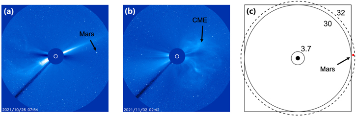
Figure 6. SOHO/LASCO C3 image. (a) 2021 October 26, 07:54. Mars's position is marked by a black arrow. (b) 2021 November 2, 02:42. The black arrow marks a CME. (c) 2021 November 2. The diagram of Mars's position in the LASCO C3 field of view. The red dot is the position of Mars.
Download figure:
Standard image High-resolution image4.2. Differential Phase Delay
DPD is obtained by using two DOR sidetones with a frequency span width of 38.4 MHz for TW1 (1 ps = 5.8 TECU). In general, people study the trend of TEC variations by continuously observing the detector's signals over several hours. However, due to the alternate observations (detector–radio source–detector), the detector's data is discontinuous. In order to obtain a better understanding of the overall trend in TEC variations, we use the method of linear fitting and extrapolation in the literature (He et al. 2022) to connect the DPD data between the scans. Before connecting, we use the continuous 2 hr observation data of TW1 on 2021 October 23 (18.4 Rs) to verify this method. After obtaining a continuous series of DPD values, we simulate the ΔDOR observing mode by intermittently removing some of the DPD data and then connecting the remaining DPD (He et al. 2022). It should be noted that after connecting the DPD data between the scans, to better illustrate the overall trend of DPD variations, we have taken the approach of subtracting the initial value from the entire data set and set the initial value to zero. Finally, we compare the connection trend of the simulated data with the actual values. In the Appendix, the result shows that the trend of changes in DPD obtained by this connection method is similar to the actual trend of changes.
To compare the variations of TEC caused by CME, we select 3 days of data with similar heliocentric distances for further study. We subtract the effect of the Earth's ionosphere. Figure 7 shows the changing trend of connected DPD on 2021 October 26, November 2, and November 9 respectively. It is found that the DPD variations are within 30 ps on both October 26 (22.1 Rs) and November 9 (39.1 Rs). On November 2 (30.6 Rs), the variation from a single scan is greater than 50 ps (290 TECU), and the overall changing trend of the TEC reaches 170 ps (986 TECU). Meanwhile, the decline of the connected DPD indicates that the TEC is increased (He et al. 2022). The DPD technique is useful to describe the CME, as demonstrated here.
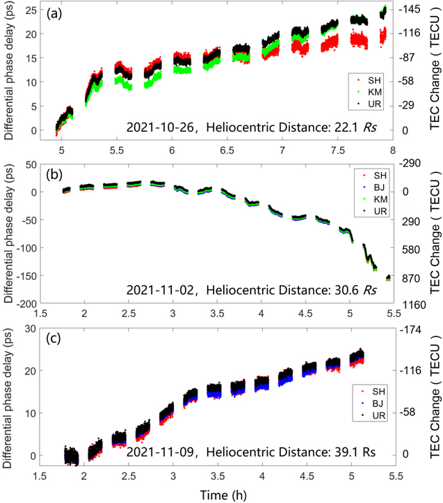
Figure 7. Connected DPDs and their corresponding TEC changes (right axes). (a) 2021 October 26, (b) 2021 November 2, (c) 2021 November 9.
Download figure:
Standard image High-resolution image4.3. CME Velocity Analysis
A frequency spike refers to a sudden and significant increase in signal frequency that exceeds the ambient data. Ma et al. (2022) shows that CMEs can cause frequency spikes that can be applied to estimate the propagation velocity of CMEs. We also find two distinctive spikes with the time lag between the arrival time at different radio telescopes in Figure 8. At both 03:02:35 and 05:12:22, the fluctuations of frequency spikes and phase spikes of all stations exceed 1 Hz and 5 rad, respectively. At 03:02:35, Figures 8(a) and (c) show that frequency spikes and phase spikes associated with the CME arrive at KM, SH, BJ, and UR successively. At 05:12:22, it can be seen from Figures 8(b) and (d) that they arrive successively at SH, KM, BJ, and UR.

Figure 8. (a) Frequency and (c) phase spikes at SH 03:02:35. (b) Frequency and (d) phase spikes at SH 05:12:22.
Download figure:
Standard image High-resolution imageTo better analyze the velocity and the directionality of the CME, we first analyze the radial and tangential projections of each baseline in the heliocentric coordinate system, as seen in Figure 9. To facilitate understanding, the projected positions of CVN stations on the ecliptic plane in heliographic coordinates are presented in Figure 10. Along the radial projection direction, SH is the closest to the Sun, followed by BJ, KM, and UR is the farthest. SH–UR is suitable for studying CME radial velocity because it has the largest radial component, greater than 1600 km, and the smallest tangential component, within 220 km. On the other hand, the radial projection distance of the BJ–KM baseline is less than 540 km, but their tangential projection distance is the largest among the six baselines, with a distance greater than 875 km, making BJ–KM suitable for studying the CME tangential velocity. Therefore, we study the direction of CME propagation by calculating the velocity of the CME on these two baselines.
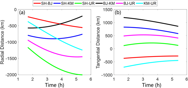
Figure 9. Projection of VLBI baselines in the heliocentric coordinate system. (a) Radial projection, (b) tangential projection.
Download figure:
Standard image High-resolution image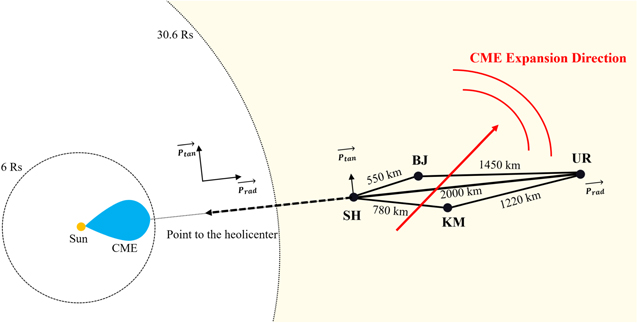
Figure 10. The projected radial and tangential distance of the baselines between the station pairs onto the ecliptic plane in heliographic coordinates are marked at SH 05:12:22. The CME first occurred in the SOHO/LASCO C2 images at 21:36 on 2021 November 1, and was observed by VLBI radio telescopes at 30.6 Rs at 03:02 on November 2.
Download figure:
Standard image High-resolution imageTypically, if the solar wind propagates radially in the ecliptic plane, the spike first reaches the SH projection point closest to the Sun, then followed by the BJ, KM, and UR projection points. However, in Figure 8(a), the spike first reaches the KM point, and in Figure 8(b), between BJ and KM, the spike also first reaches the KM point. This suggests that, in addition to radial velocity, CME has tangential velocity when propagating toward the solar north pole.
As shown in Table 3, the radial and tangential propagation velocities of the solar wind are estimated separately using the SH–UR and BJ–KM baselines. We use the output of PLL with an integration time of 10 ms to calculate the velocity of the CME. As a comparison, we also use cross correlation method to calculate CME velocity (Ma et al. 2021, 2022). The correlation coefficients between the two stations are greater than 0.9. The error bars are determined as half of the difference between the velocities obtained from the two calculation methods.
Table 3. The Velocity of Solar Wind Measured by the Visual Frequency Spikes and Cross Correlation
| Time | Spikes | Lag | vrad1 a |
 b
b
| vrad2 c |
 d
d
|
|---|---|---|---|---|---|---|
| (Hz) | (s) | (km s−1) | (km s−1) | (km s−1) | (km s−1) | |
| SH 03:02:35.925 | 1.15 | −1.72 | 950 ± 37.0 | ... | 1024 ± 37.0 | ... |
| UR 03:02:37.645 | 1.09 | |||||
| BJ 03:02:36.915 | 1.16 | 1.16 | ... | 945 ± 9.5 | ... | 926 ± 9.5 |
| KM 03:02:35.755 | 1.10 | |||||
| SH 05:12:22.725 | −1.66 | −2.87 | 697 ± 22.5 | ... | 742 ± 22.5 | ... |
| UR 05:12:25.595 | −1.75 | |||||
| BJ 05:12:23.855 | −1.80 | 0.63 | ... | 1393 ± 58.5 | ... | 1510 ± 58.5 |
| KM 05:12:23.225 | −1.97 |
Notes.
a vrad1 means the radial velocity of the CME obtained by visual frequency spikes. b means the tangential velocity of the CME obtained by visual frequency spikes.
c
vrad2 means the radial velocity of the CME obtained by cross correlation.
d
means the tangential velocity of the CME obtained by visual frequency spikes.
c
vrad2 means the radial velocity of the CME obtained by cross correlation.
d
 means the tangential velocity of the CME obtained by cross correlation.
Download table as: ASCIITypeset image
The CME observed in our study is CME 7 in Li et al. (2022). The time when the CME first occurred in the SOHO/LASCO C2 images is at 21:36 on 2021 November 1. After 5.5 hr of propagation, this CME reached the signal transmission path at 30 Rs and was observed by us. From the above two spikes, at SH 03:02:35, the radial velocity vrad on the SH–UR baseline and tangential velocity vtan on the BJ–KM baseline of CME are 987 ± 37.0 and 935.5 ± 9.5 km s−1, respectively, which is consistent with the velocity of 1014 ± 15 km s−1 reported by Li et al. (2022). At SH 05:12:22, vtan on the BJ–KM baseline is twice as fast as vrad on the SH–UR baseline, with values of 1451.5 ± 22.5 and 720 ± 22.5 km s−1, respectively. These two velocities are inconsistent with the results in Li et al. (2022). This difference in time lag and velocity can be attributed to the instantaneous velocity variations of the CME. Figure 10 shows that the CME is propagating in a direction approximately 45° offset from the radial projection from SH–UR toward the north pole in the heliocentric coordinate system. Meanwhile, we also observe a similar directional expansion of the CME in the LASCO C3 observation images, which is consistent with the analysis of velocity in this work.
It should be noted that this study employs a different method to measure CME velocities compared to Li et al. (2022). Li et al. (2022) utilized the graduated cylindrical shell modeling technique and analyzed several hours of STEREO-A COR2 and LASCO C2 coronagraph images to perform three-dimensional modeling of the CME. Due to the limited field of view of the coronagraph, the average velocity of the CME front they obtained is within 6 Rs. As a supplementary point, we use the multiground VLBI radio telescopes to detect the instantaneous velocities and density structure of the same CME at 30 Rs in the interplanetary space. From Figures 5 and 8, we can see that the frequency and phase of the spacecraft are very sensitive to the density variations of the CME, and the frequency spikes appeared because of the density contrast between the transient inhomogeneities and the ambient flow. The different appearance time of spikes at different telescopes indicates the dynamic propagation of the solar wind density structures along the spatial projection baselines. The projections along radial and latitudinal directions give the two-dimensional velocity of the CME. This method is also effective at detecting the oscillation and propagation of the nascent dynamic solar wind structure near the Sun, e.g., at 2.6 Rs (Ma et al. 2022). As a matter of fact, the density disturbance of the CME is the integration effects along the direction of the signal transmission path. However, when using spikes to calculate the velocity of the CME, we assume that the spikes are only caused by the density disturbance at the solar proximate point on the ray path. Therefore, this simplified model results in certain estimation errors. Nevertheless, comparison with Li et al. (2022) and SOHO/LASCO shows our method can be used to estimate the propagation direction and velocity of a CME with reasonable accuracy.
5. Conclusion
TW1 is China's first Mars probe successfully launched and landed on Mars. In this study, we investigate the application of DOR signals of TW1 in researching solar wind plasma and CME. We obtain the phase and frequency of the DOR carrier and sidetone signals from the CVN observation data using third-order PLL. We also use the sidetone signals to calculate the single-station DPD and TEC. We then perform statistical analysis on the impact of solar wind plasma on the probe signals at different heliocentric distances. The results show that as the heliocentric distance decreases, the frequency, phase, ΔDOR group delay, delay rate, and TEC all show increasing fluctuations.
Comparing the single-station DPD with LASCO C3, we confirm the detection of one CME passing through the ray paths on 2021 November 2. Meanwhile, we employ frequency scintillation and cross correlation methods to calculate the velocity variations of the CME. The velocity of the detected CME at 30 Rs is consistent with that of the same CME within 6 Rs, which initially appeared in the SOHO/LASCO C2 images at 21:36 on 2021 November 1 (Li et al. 2022). Furthermore, the velocity variations caused by the density disturbances is also detected by us. Notably, from the above study we find that the distribution of the CVN baseline is well suited to studying the solar wind. The SH–UR baseline is east–west oriented, making it well suited for studying the radial velocity of the solar wind in the heliocentric coordinate system at low latitudes. On the other hand, the north–south orientation of the BJ–KM baseline makes it suitable for studying the tangential velocity perpendicular to the radial direction.
This study has great value for future application in China's deep-space exploration to monitor the interplanetary space environment and study the influence of solar wind on the orbit determination of deep-space probes.
Acknowledgments
We thank CVN including the Shanghai, Beijing, Kunming, Urumqi, and Tianma stations, and the VLBI Center for participating in the TW1 observation and providing the data required for this study. The SOHO/LASCO data used here are produced by a consortium of the Naval Research Laboratory (USA), Max-Planck-Institut für Sonnensystemforschung (Germany), Laboratoire d'Astronomie (France), and the University of Birmingham (UK). SOHO is a project of international cooperation between ESA and NASA. This work was supported by grants 12273098, 11973074, 42241118, and 11803069 from the National Natural Science Foundation of China, Shanghai Key Laboratory of Space Navigation and Position Techniques, and Key Laboratory of Radio Astronomy of CAS.
Appendix:
We observe the probe for 2 hr on 2021 October 23 and obtain the DPD (1 ps = 11.7 TECU) by using the main carrier and the sidetone which is equal to the main carrier frequency adding 19.2 MHz. The overall change trend of DPD is 18 ps (210 TECU). We delete the DPD data at equal intervals by simulating the observation mode of differential VLBI (9 minutes probe, 7 minutes interval), and connect the remaining data according to the He et al. (2022) method.
The results are shown in Figure 11. It can be observed that the trend of the simulated data after the connection is nearly consistent with the actual trend of changes for the DPD data observed within 2 hr. Although the values cannot completely overlap, the maximum gap is 3 ps (35 TECU), which does not affect the overall trend. Therefore, it can be concluded that the connection method is reliable when the probe's observation scans are long enough, and the interval between scans is short.

Figure 11. Differential phase delays and their corresponding TEC changes (right axis) on 2021 October 23.
Download figure:
Standard image High-resolution image