


Abstract
The photodissociation of O2 is thought to play a vital role in blocking UV radiation in the Earth's atmosphere and likely has great importance in characterizing exoplanetary atmospheres. This work considers four photodissociation processes of O2 associated with its four electronic states, whose potential energy curves and transition dipole moments are calculated at the icMRCI+Q/aug-cc-pwCV5Z-DK level of theory. The quantum-mechanical approach is used to compute the state-resolved cross sections for two triplet transitions from the ground X  state to the excited B
  and E
and E  states, and for two singlet transitions from the a 1Δg and b
  states to the 1 1Πu state, with a consideration of photon wavelengths from 500 Å to the relevant threshold. Assuming the populations of the initial states satisfy a Boltzmann distribution, the temperature-dependent photodissociation cross sections are estimated at gas dynamic temperatures of 0–10,000 K, in which the discrete progressions of the B
 and E
and E 
 transitions are also considered. The photodissociation rates of O2 in the interstellar, solar, and blackbody radiation fields are also calculated using the temperature-dependent cross sections. The resulting photodissociation cross sections and rates are important for the atmospheric chemistry of Earth and may be also useful for the atmospheric exploration of exoplanets.
Export citation and abstract BibTeX RIS

Original content from this work may be used under the terms of the Creative Commons Attribution 4.0 licence. Any further distribution of this work must maintain attribution to the author(s) and the title of the work, journal citation and DOI.
1. Introduction
Oxygen (O) is the third most plentiful element in the universe, after hydrogen and helium (Hollenbach et al. 2009). Dioxygen (O2) is the second most plentiful molecule in the Earth's atmosphere (Krupenie 1972; Huebner et al. 1975) and the fourth most abundant molecule in cometary material (Bieler et al. 2015; Taquet et al. 2016; Keeney et al. 2017; Yao & Giapis 2017; Luspay-Kuti et al. 2018; Taquet et al. 2018). O2 is involved in the geochemistry (Bender & Grande 1987; Birkham et al. 2003; Qiu et al. 2023) and atmospheric photochemistry of Earth and Mars (Barker 1972; Yeung et al. 2016; Lefèvre & Krasnopolsky 2017; Gregory et al. 2021). O2 has been identified in molecular clouds and star-forming regions (Larsson et al. 2007; Goldsmith et al. 2011; Liseau et al. 2012; Pezzella & Meuwly 2019). O2 is also a component of stellar atmospheres (Krupenie 1972; Hays & Roble 1973; Amarsi et al. 2016). In particular, O2 acts as a biosignature in exoplanetary atmospheres and its spectroscopic and photochemical signatures are key to finding life on exoplanets (Meadows 2017; Fujii et al. 2018; Meadows et al. 2018).
Here, we concentrate on one photochemical process (namely photodissociation) of O2. After absorbing the energy of a photon, O2 can be excited from a lower bound state to an upper free state, which is then accompanied by dissociation into two atomic O fragments. Here is an example, as follows:

Such a process is known as photodissociation. Photodissociation is an essential mechanism for molecular destruction and is crucial in modeling the evolution of chemical composition in regions with intense UV radiation (Pattillo et al. 2018). Experimental photoabsorption (including photodissociation and photoionization) cross sections are usually obtained directly by observing the transmission of an UV continuum spectrum through a gas sample. A detailed overview of experimental photoabsorption cross sections can be seen in several previous publications (Heays et al. 2017; Hrodmarsson & van Dishoeck 2023). The theory and methodology of photodissociation for diatomic molecules and ions are well summarized in previous works (Kirby & Van Dishoeck 1989; Heays et al. 2017; Hrodmarsson & van Dishoeck 2023). These computational methods are based on quantum mechanics and have been used to deal with the photodissociation processes of many diatomic molecules or ions, such as CS (Pattillo et al. 2018), CN (El-Qadi & Stancil 2013), SH+ (McMillan et al. 2016), BeH+ (Yang et al. 2020), HeH+ (Miyake et al. 2011), AlH (Qin et al. 2021a), AlCl (Qin et al. 2021b), AlF (Qin et al. 2022b), MgO (Bai et al. 2021), MgH (Weck et al. 2003), HCl and HF (Qin et al. 2022a), etc. Recently, the ExoMol group have provided a new treatment for calculating photodissociation cross sections and rates (Pezzella et al. 2021, 2022).
The photodissociation of O2 is a crucial process for blocking the UV irradiation in the Earth's atmosphere and it can also impact some natural phenomena, such as auroras, the airglow, and the nightglow, etc. (Savigny 2017; Gao et al. 2020; Lednyts'kyy 2020; Lednyts'kyy & von Savigny 2020; Royer et al. 2021). Moreover, the photodissociation of O2 is the first step of the "Chapman cycle." O2 and its photolysis products can provide essential components needed for a number of subsequent chain reactions and other complex reactions. The resulting oxygen–ozone cycle system provides a natural protective barrier for life activities on Earth. Therefore, photodissociation studies of O2, including photodissociation cross sections and rates, are essential for modeling the atmospheric photochemistry. Most of the existing experimental and theoretical studies focus on the Schumann–Runge continuum (B 
 ; 100–176 nm), the Schumann–Runge band (B
 ; 176–200 nm), and the Herzberg continuum (200–242 nm). An early study of the absorption spectrum of the Schumann–Runge band was measured by Ackerman et al. (1970). Considering the effect of temperature, Gibson et al. (1983) measured the photoabsorption cross sections of the Schumann–Runge continuum in the range of 295–575 K. Allison et al. (1986) developed a semi-empirical model of the Schumann–Runge continuum and presented photodissociation cross sections in the wavelength range of 127–152 nm. Later, Yoshino et al. (1992) measured the absorption cross sections of the Schumann–Runge band in the window region between the rotational lines. Balakrishnan et al. (2000) studied the predissociation process in the Schumann–Runge continuum using a time-dependent quantum mechanical method. Using the coupled-channel Schrödinger equations method, Lewis et al. (2001) presented the photodissociation cross sections for the Schumann–Runge continuum and discrete Schumann–Runge band of O2. In addition, there are also many studies on the Herzberg continuum (Buijsse et al. 1998; van Vroonhoven & Groenenboom 2002a, 2002b; Alexander et al. 2003; Brouard et al. 2006; Chestakov et al. 2010). Recently, the Leiden photodissociation & photoionization cross section database (Heays et al. 2017; Hrodmarsson & van Dishoeck 2023) carefully collected and selected the photodissociation cross sections of O2 from previous studies and its uncertainty was judged to be about 30%. Overall, there are no comprehensive O2 photodissociation cross sections and rates for simultaneously considering multiple electronic transitions and different temperature ranges, so a systematic study of the O2 photodissociation is necessary.
In this work, photodissociation cross sections from the lowest three electronic states of O2 to the excited states are calculated using quantum mechanical methods, specifically including the transitions from the ground X  state to the B
  and E
and E  states and those from the a 1Δg and b
  states to the 1 1Πu state. The temperature-dependent cross sections are then computed assuming the initial rovibrational energy levels for the X
  , a 1Δg, and b
  states conform to the Boltzmann distribution. Finally, photodissociation rates in the standard interstellar radiation field (ISRF), solar radiation field, and blackbody radiation field are provided over a wide range of temperatures.
2. Theory and Methods
2.1. Ab Initio Calculation
Implementing the high-level ab initio calculations in the MOLPRO 2015 software package (Werner et al. 2015, 2020), potential energy curves (PECs) and transition dipole moments (TDMs) of O2 have been obtained. For a homonuclear diatomic molecule like O2 with D∞h symmetry, MOLPRO cannot take advantage of the full symmetry of the non-Abelian group, so the Abelian subgroup D2h is chosen. The relationships of the irreducible representations from D∞h to D2h are as follows:  → Ag,
→ Ag,  → B1g,
  → B1u,
  → Au, Πu → B2u/B3u, Πg → B2g/B3g, Δg → Ag/B1g, and Δu → Au/B1u. The computational steps are conventional. First of all, the Hartree–Fock calculation was used for the ground X
  state of O2 to generate the initial single-configuration wave function and energy. Then, the complete active space self-consistent field (CASSCF) method (Knowles & Werner 1985; Werner & Knowles 1985) was used to optimize the initial wave function to obtain the multiconfiguration wave function. Finally, the dynamic correlation effect of O2 was calculated using the internally contracted multireference configuration interaction (icMRCI) method (Knowles & Werner 1988, 1992; Werner & Knowles 1988; Shamasundar et al. 2011) based on the CASSCF wave function, and the Davidson correction (+Q) was also contained to take into account the size-consistency error (Langhoff & Davidson 1974). All the calculations of the PECs and TDMs for O2 were performed with the augmented correlation-consistent polarized weighted core–valence aug-cc-pwCV5Z-DK basis set (Peterson & Dunning 2002).
The electronic arrangement of O is 1s22s22p4. For O2, the electrons in the 1s shell were treated as closed, and the electrons in the remaining shells were put into the active space. Extra virtual orbitals were also added for better relaxation of the wave functions of high-lying electronic states. The set of orbitals is composed of four Ag orbitals, two B3u orbitals, two B2u orbitals, zero B1g orbitals, four B1u orbitals, one B2g orbital, one B3g orbital, and zero Au orbitals and it is denoted as (4, 2, 2, 0, 4, 1, 1, 0). For the singlet and ground X  states, we consider the internuclear distances between 0.9 and 6.0 Å. For the remaining triplet states, the internuclear distances from 1.0 to 6.0 Å are chosen. The step sizes are 0.02 Å for the internuclear distances from 1.0 to 2.5 Å and 0.05 Å for other internuclear distances.
2.2. Photodissociation Theory
The theory of photodissociation for diatomic molecules has been described in detail in previous works (Kirby & Van Dishoeck 1989; El-Qadi & Stancil 2013; Heays et al. 2017; Pattillo et al. 2018). Here we present a brief overview for the calculation of photodissociation cross sections and rates.
In units of cm2 molecule−1, the state-resolved cross section for a bound → free transition from the initial rovibrational level υ''N'' is
where Eph is the photon energy in atomic units,  are the Hönl–London factors (Kovács & Nemes 1969), the term
  is the degeneracy factor, and Λ is the angular momentum projections along the molecular axis. J, υ, and N are the total angular, vibrational, and rotational momentum quantum numbers, respectively. The initial state is denoted with a single prime superscript and the final state with a double prime.
In Equation (2),  is the electron transition dipole matrix element, given by

where D(R) is the electronic TDM in atomic units,  (R) is the continuous wave function of the final state, and χυ''N'' (R) is the bound wave function of the initial state.
For the case in which a Boltzmann distribution is assumed for the rovibrational levels of the initial electronic state, the corresponding total photodissociation cross section is a function of both temperature T and wavelength λ, and can be expressed as

where Q(T) is the rovibrational partition function, expressed as
where En υ N is the energy of the nth electronic state with quantum numbers υ, N and ε0 refers to the energy of the lowest energy level. S is the spin quantum number. h, kB, and c are the Planck constant, Boltzmann constant, and the speed of light in vacuum, respectively.
The photodissociation rate k of a molecule exposed to a UV radiation field can be estimated using the photodissociation cross sections σ(λ), given by

where I (λ) is the sum of the photon intensities from the radiation field at all angles of incidence. The photon radiation intensity surrounded by a blackbody at the temperature of Trad is expressed as

where h is the Planck constant and c is the speed of light. As inspired by Heays et al. (2017) and Pezzella et al. (2022), we take into account the blackbodies of three distinct temperatures to define various sorts of stars. T Tauri stars and stars in their early stages (Appenzeller & Mundt 1989; Natta 1993) are modeled using the blackbody of Trad = 4000 K. To model the Herbig Ae stars and young A stars still encased in gas and dust (Vioque et al. 2018), the blackbody of Trad = 10,000 K was selected. The brilliant and fleeting B stars (Habets & Heintze 1981) are modeled using the blackbody of Trad = 20,000 K. It is worth noting that the blackbody radiation fields are normalized in this work to match the ISRF's energy intensity between 91.2 and 200 nm, as treated by Heays et al. (2017) and Pezzella et al. (2022). The scaling factors of 3.627 × 10⁸, 5.786 × 10¹³, and 6.109 × 10¹⁵ are used for the photodissociation rates in the radiation fields of the blackbody bodies for Trad = 4000 K, Trad = 10,000 K, and Trad = 20,000 K, respectively.
For the standard ISRF, the photodissociation rate is computed using the wavelength dependence UV intensity defined by Draine (1978) at wavelengths of 91.2 < λ < 200 nm and extended by van Dishoeck & Black (1982) for λ > 200 nm. The solar radiation field was drawn from Heays et al. (2017) and its intensity was originally compiled from the data that were measured by Woods et al. (1996) and Curdt et al. (2001). A scaling factor of 37,700 should be used to increase the solar photodissociation rates calculated here to values appropriate for the approximate solar intensity at a distance of 1 au from the Sun.
3. Results and Discussion
3.1. PECs and TDMs
In this work, six electronic states of O2 correlating to the lowest two dissociation limits have been calculated and shown in Figure 1 as a function of the internuclear distance R, including three singlet states (i.e., a 1Δg, b  , and 1 1Πu) and three triplet states (i.e., X
  , B
, B  , and E
  ). The X
  , a 1Δg, b
  , and 1 1Πu states converge to the first dissociation limit O (2s22p4
3P) + O (2s22p4
3P) and the B
, and 1 1Πu states converge to the first dissociation limit O (2s22p4
3P) + O (2s22p4
3P) and the B  and E
and E  states correlate to the second dissociation limit O (2s22p4
3P) + O (2s22p4
1D). The computed energy of the second dissociation limit relative to the first one is 15,745.11 cm−1, which is only 122.75 cm−1 (0.77%) smaller than the experimental value (Kramida et al. 2022). Liu et al. (2014) pointed out the existence of a double potential well in the B
states correlate to the second dissociation limit O (2s22p4
3P) + O (2s22p4
1D). The computed energy of the second dissociation limit relative to the first one is 15,745.11 cm−1, which is only 122.75 cm−1 (0.77%) smaller than the experimental value (Kramida et al. 2022). Liu et al. (2014) pointed out the existence of a double potential well in the B  state. We guess that the double potential well obtained by Liu et al. (2014) may come from the root flipping, i.e., the calculational energy points of the B
  and 2 3Δu states interchange with each other (at about 2.0 Å). To avoid root flipping, we performed state-averaged calculations of the first four electronic states with the same symmetry as the B
  state. The results show that the B
  state has a single potential well. Moreover, adiabatic B
  and E
and E  states avoid crossing at about 1.2 Å near the equilibrium internuclear of the ground state, as shown in Figure 1(a). These interactions produce large gradients in the coupling curves connecting these states within the region of the avoided crossing, as shown for the TDMs in Figure 2.

Figure 1. PECs of (a) the X  , B
, B  1, and E
  states and (b) the a 1Δg, b
  , and 1 1Πu states for O2.
Download figure:
Standard image High-resolution image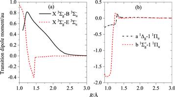
Figure 2. TDMs for (a) the triplet and (b) singlet transitions of O2.
Download figure:
Standard image High-resolution imageTable 1 presents the spectroscopic constants of the X  , a 1Δg, b
  , and B
  states, including the dissociation energy De
, the electronic excitation energy relative to the ground state Te
, the equilibrium internuclear distance Re
, the harmonic frequency ωe
, the first-order anharmonic constant ωe
χe
, the rotational constant Be
, and the rovibrational coupling constant αe
. These spectroscopic constants were obtained by fitting the rovibrational levels determined by solving the nuclear motion equation over the PECs. Previous experimental and theoretical results were also provided for comparison.
states, including the dissociation energy De
, the electronic excitation energy relative to the ground state Te
, the equilibrium internuclear distance Re
, the harmonic frequency ωe
, the first-order anharmonic constant ωe
χe
, the rotational constant Be
, and the rovibrational coupling constant αe
. These spectroscopic constants were obtained by fitting the rovibrational levels determined by solving the nuclear motion equation over the PECs. Previous experimental and theoretical results were also provided for comparison.
Table 1. Spectroscopic Constants of the X  , B
, B  , a 1Δg, and b
  States for O2 along with Available Experimental and Theoretical Values
| State | Source | De | Te | Re | ωe | ωe χe | Be | αe |
|---|---|---|---|---|---|---|---|---|
| (eV) | (cm−1) | (Å) | (cm−1) | (cm−1) | (cm−1) | (cm−1) | ||
X 
| This work | 5.2070 | 0 | 1.2089 | 1578.72 | 12.5967 | 1.4438 | 0.0161 |
| Exp. a | 5.2132 | 0 | 1.2075 | 1580.19 | 11.98 | 1.4456 | 0.0159 | |
| Exp. b | 5.213 | 0 | 1.208 | 1580.2 | 11.98 | 1.45 | 0.0159 | |
| Calc. c | 5.2203 | 0 | 1.2068 | 1581.61 | 10.039 | 1.4376 | 0.0125 | |
| Calc. d | 4.957 | 0 | 1.236 | 1498.8 | 9.87 | 1.38 | 0.0141 | |
B 
| This work | 1.0087 | 49,502.50 | 1.6071 | 701.49 | 7.5962 | 0.8123 | 0.0103 |
| Exp. a | 49,793.28 | 1.6042 | 709.31 | 10.65 | 0.8190 | 0.0121 | ||
| Exp. b | 1.007 | 49,794.33 | 1.604 | 709.1 | 10.61 | 0.819 | 0.0119 | |
| Calc. c | 0.8417 | 51,028.73 | 1.5978 | 723.60 | 10.756 | 0.8256 | 0.0136 | |
| Calc. d | 1.136 | 49,030.42 | 1.627 | 724.9 | 7.04 | 0.791 | 0.0077 | |
| a 1Δg | This work | 4.2538 | 7800.12 | 1.2187 | 1515.08 | 13.1273 | 1.4237 | 0.0169 |
| Exp. a | 7918.1 | 1.2156 | 1483.5 | 12.9 | 1.4263 | 0.0171 | ||
| Exp. b | 4.231 | 7918.11 | 1.216 | 1509.3 | 12.9 | 1.43 | 0.0171 | |
| Calc. c | 4.2258 | 7776.43 | 1.2147 | 1491.07 | 8.1245 | 1.3814 | 0.0042 | |
| Calc. d | 3.857 | 8855.96 | 1.250 | 1403.4 | 8.74 | 1.35 | 0.0158 | |
| b 1Σ+ g | This work | 3.6658 | 12,951.19 | 1.2273 | 1449.98 | 16.4295 | 1.3981 | 0.0182 |
| Exp. a | 1.2269 | 1432.77 | 14.00 | 1.4004 | 0.0182 | |||
| Exp. b | 3.577 | 13,195.31 | 1.227 | 1432.7 | 13.93 | 1.40 | 0.0182 | |
| Calc. c | 3.6058 | 13,099.92 | 1.2258 | 1438.65 | 12.723 | 1.4030 | 0.0180 | |
| Calc. d | 3.168 | 14,324.40 | 1.267 | 1310.8 | 10.44 | 1.31 | 0.0172 |
Notes.
a Huber & Herzberg (1979). b Krupenie (1972). c Liu et al. (2014). d Saxon & Liu (1977).Download table as: ASCIITypeset image
For the ground X  state, the equilibrium internuclear distance Re
of 1.2089 Å is slightly larger than the experimental values of 1.2075 Å (Huber & Herzberg 1979) and 1.208 Å (Krupenie 1972) and agrees well with the theoretical results with relative errors of 0.17% (Liu et al. 2014) and 2.19% (Saxon & Liu 1977). The calculated harmonic frequency ωe
is 1578.72 cm−1, which differs from the experimental value by 1.47 cm−1 with a relative error of 0.09% (Huber & Herzberg 1979) and differs from the recent theoretical value by 2.89 cm−1 with a relative error of 0.18% (Liu et al. 2014). For the rotational constant Be
and rovibrational coupling constant αe
, the errors relative to the experimental values (Huber & Herzberg 1979) are 0.12% and 0.94%, respectively. For the a 1Δg and b
state, the equilibrium internuclear distance Re
of 1.2089 Å is slightly larger than the experimental values of 1.2075 Å (Huber & Herzberg 1979) and 1.208 Å (Krupenie 1972) and agrees well with the theoretical results with relative errors of 0.17% (Liu et al. 2014) and 2.19% (Saxon & Liu 1977). The calculated harmonic frequency ωe
is 1578.72 cm−1, which differs from the experimental value by 1.47 cm−1 with a relative error of 0.09% (Huber & Herzberg 1979) and differs from the recent theoretical value by 2.89 cm−1 with a relative error of 0.18% (Liu et al. 2014). For the rotational constant Be
and rovibrational coupling constant αe
, the errors relative to the experimental values (Huber & Herzberg 1979) are 0.12% and 0.94%, respectively. For the a 1Δg and b  states, their spectroscopic constants are in good agreement with the experimental values (Huber & Herzberg 1979) and the theoretical ones (Liu et al. 2014). For the B
  state, our calculations obviously improve the spectroscopic constants relative to those calculated by Liu et al. (2014), by comparing with the experimental values (Huber & Herzberg 1979). Such improvement may be attributable to the high-level icMRCI/aug-cc- pwCV5Z-DK calculation.
Dipole-allowed TDMs between the abovementioned six electronic states are shown in Figure 2 as a function of the internuclear distance R. Figure 3 compares the TDMs of the B 
 transition with previous results. The TDM for the B
 transition shows the same trend as those computed by Allison et al. (1986) and Liang et al. (2020) for R larger than 1.24 Å. For R smaller than about 1.24 Å, our TDM exhibits a similar trend to that given by Allison et al. (1986), but different from that presented by Liang et al. (2020). Such difference corresponds to different PECs of the B
  state, in which we considered the avoided crossing with the E
  state.
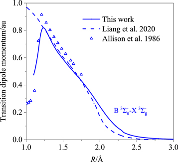
Figure 3. Comparison of TDMs for the B 
 transition with those computed by Liang et al. (2020) and Allison et al. (1986).
Download figure:
Standard image High-resolution imageTo better reproduce the spectrum of the Schumann–Runge band, we use the CHIPR program (Rocha & Varandas 2019, 2020, 2021; Chen et al. 2022,
2023; Li et al. 2022, 2023) in combination with experimental energy levels (Krupenie 1972) to refine the PECs of the B  and X
and X  states. Here, we present a brief overview for the theory of this method.
In the CHIPR method, the diatomic PEC assumes the following form:

where ZA and ZB are the nuclear charges for the atoms A and B, and yk is expanded as

where cα are contraction coefficients, with α establishing the primitive functions' indexes ϕp,α . ϕp,α have the following two expressions:

and

where ρp,α
is the deviation of the coordinate Rp
from the primitive origin  ,
,  . γp,α
are nonlinear parameters, ηα
= 1, βα
= 6, and σα
= 1/5. The distributed origins
. γp,α
are nonlinear parameters, ηα
= 1, βα
= 6, and σα
= 1/5. The distributed origins  can be expressed by

where ζ and  need to be carefully chosen while fitting.
The refined PECs for the X  and B
and B  states are shown in Figures 4(a) and 5(a), respectively. The errors between the vibrational-level energies obtained from our experimentally refined PECs and previously measured ones are shown in Figures 4(b) and 5(b) for the X
  and B
and B  states, respectively. The maximum errors for the X
  and B
and B  states are 0.99 cm−1 and 2.35 cm−1, respectively. The experimental vibrational levels come from Krupenie (1972). For the E
  state, its electronic excitation energy Te
was first shifted to be the estimated value of 79,800 cm−1 from Huber & Herzberg (1979), but the resulting line position for the peak of the cross sections for the E
state, its electronic excitation energy Te
was first shifted to be the estimated value of 79,800 cm−1 from Huber & Herzberg (1979), but the resulting line position for the peak of the cross sections for the E 
 transition slightly deviates from that of the more recent measurement by Lu et al. (2010). Hence, we adjusted the Te
of the E
transition slightly deviates from that of the more recent measurement by Lu et al. (2010). Hence, we adjusted the Te
of the E  state to be 79,643 cm−1 to better reproduce the observation by Lu et al. (2010).
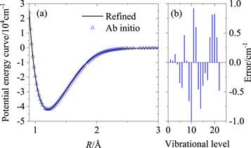
Figure 4. (a) The PEC for the ground X  state. The open triangles are ab initio energy points. The solid line represents the experimentally refined curve by the CHIPR program. (b) The errors between the vibrational-level energies obtained from our experimentally refined PEC and the experimental ones.
Download figure:
Standard image High-resolution image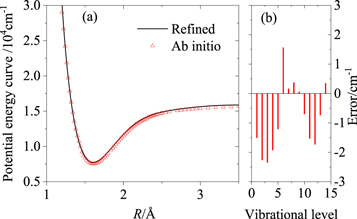
Figure 5. (a) The PEC for the B  state. The open triangles are ab initio energy points. The solid line represents the experimentally refined curve by the CHIPR program. (b) The errors between the vibrational-level energies obtained from our experimentally refined PEC and the experimental ones.
Download figure:
Standard image High-resolution imageTo calculate the photodissociation cross sections and rates, ab initio PECs and TDMs are needed to be interpolated and extrapolated. For short-range internuclear distances at R< 0.9 Å, an exponential function is used for extrapolation, given by

where A, B, and C are fitting parameters. For long-range internuclear distances at R > 6 Å, the following formula is used for extrapolation:

where C5 and C6 are fitting coefficients, which are approximately estimated in this work. C6 was calculated using the London formula:

where ΓO and αO are the ionization energy and static dipole polarizability, respectively, for a specific electronic state of the O atom. ΓO can be obtained from the NIST Atomic Spectroscopic Database (Kramida et al. 2022). The dipole polarizabilities of the oxygen atoms in the 3P and 1D states are 5.35 and 5.43 au, respectively, computed by Medveď et al. (2000). C5 was estimated by fitting ab initio points while keeping C6 and the dissociation limits fixed. A cubic spline was used to interpolate the ab initio points. A similar treatment was used in previous publications (Pattillo et al. 2018; Babb et al. 2019; Meng et al. 2022; Zhang et al. 2022).
3.2. State-resolved and Temperature-dependent Cross Sections
State-resolved cross sections are the basis for a detailed study of the temperature-dependent photodissociation cross sections and rates. State-resolved photodissociation cross sections from the initial rovibrational energy level (υ'', N'') = (0, 1) of the ground X  state to the excited B
  and E
and E  states, and from the initial rovibrational energy level (υ'', N'') = (0, 0) of the a 1Δg and b 1Σ+
g states to the 1 1Πu state, are calculated and shown in Figure 6 for photon wavelengths from 500 Å to the corresponding thresholds. The well-known Schumann–Runge continuum band of B
states, and from the initial rovibrational energy level (υ'', N'') = (0, 0) of the a 1Δg and b 1Σ+
g states to the 1 1Πu state, are calculated and shown in Figure 6 for photon wavelengths from 500 Å to the corresponding thresholds. The well-known Schumann–Runge continuum band of B 
 plays a major role at larger wavelengths between about 1200 and 1800 Å, in which the 1 1Πu ←a 1Δg and 1 1Πu ←b 1Σ+
g transitions exhibit some peaks, while the populations of the a 1Δg and b 1Σ+
g states are smaller relative to that of the ground X
plays a major role at larger wavelengths between about 1200 and 1800 Å, in which the 1 1Πu ←a 1Δg and 1 1Πu ←b 1Σ+
g transitions exhibit some peaks, while the populations of the a 1Δg and b 1Σ+
g states are smaller relative to that of the ground X  state in a general condition.
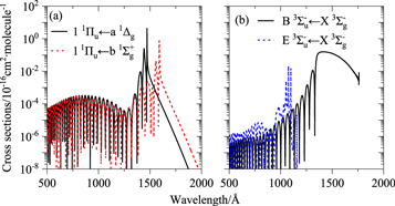
Figure 6. State-resolved cross sections of O2 for transitions from (a) the rovibrational level (υ'', N'') = (0, 0) of the a 1Δg and b 1Σ+
g states and (b) the rovibrational level (υ'', N'') = (0, 1) of the X  state.
Download figure:
Standard image High-resolution imageAssuming the populations of the initial rovibrational levels for the X  , a 1Δg, and b
  states satisfy a Boltzmann distribution, temperature-dependent cross sections were calculated for four electronic transitions of O2 at temperatures from 0 to 10,000 K in intervals of 100 K. Note that we also consider the discrete progressions for the B
 and E
and E 
 transitions, whose cross sections are calculated by the DUO and EXOCROSS programs (Yurchenko et al. 2016, 2018) and then smoothed using a normalized Gaussian function proposed by the ExoMol group (Pezzella et al. 2021, 2022). Figure 7 shows the photodissociation cross sections of four transitions of O2 at 300 K, along with those compiled by Heays et al. (2017). For wavelengths from 490 to 1080 Å, the photodissociation cross sections come from transitions into Rydberg states (Holland et al. 1993). Ogawa & Ogawa (1975) pointed out the cross sections at wavelengths from 1080 to 1150 Å might come from the absorption of the a 1Δg state. The positions of the peaks show the final state should lie higher than the 1 1Πu state. For wavelengths from 1150 to 1790 Å, the cross sections come from the absorption spectra at 303.7 K measured by Lu et al. (2010), which results from the E
 and B
and B 
 transitions. Both Lu et al. (2010) and Ogawa & Ogawa (1975) assigned the peak value at 120.54 nm to be the transition from the a 1Δg state. Our calculations guess that this peak may be due to the E
 transition. For wavelengths from 1790 to 2030 Å, the Schumann–Runge band is dominant and its cross sections are chosen from Yoshino et al. (1992). For wavelengths from 2050 to 2400 Å, the cross sections come from the Herzberg continuum presented by Yoshino et al. (1988). Overall, our photodissociation cross sections show reasonable agreement with the experimental ones for wavelengths from 1150 to 2030 Å. For wavelengths below 1150 Å, except for the direct photodissociation to high electronic states, the predissociation from nonadiabatic couplings and absorption to the Rydberg states may be also important, but these are not considered in this work.

Figure 7. Photodissociation cross sections for (a) triplet and (b) singlet electronic transitions and two discrete progressions of B 
 and E
and E 
 for O2 at 300 K. The peak heights of the discrete transitions depend greatly on the Gaussian smoothing function adopted, while the integral of the cross sections is conserved. The experimental cross section (Heays et al. 2017) is also provided for comparison.
Download figure:
Standard image High-resolution imageIn DUO calculations of the discrete transitions for the B 
 and E
and E 
 systems, 60, 20, and 3 vibrational basis functions are considered. The generated line lists for the B
 and E
and E 
 transitions are given in Tables 2 and 3, respectively. Based on the generated line lists, several spectra were calculated and compared to available laboratory measurements. Figure 8 compares the absorption spectra for the Schumann–Runge bands of O2 with the experimental ones from Yoshino et al. (1987) and Yoshino et al. (1992), showing a satisfactory agreement. The spectra are simulated at the effective temperatures of 79 and 300 K, respectively, in Figures 8(a) and (b). In Figure 9, we simulate the absorption spectra for the E
 bands of O2 at temperatures of 38 and 303.7 K, respectively, to provide direct comparison with the experimental spectra from Lu et al. (2010). The overall agreement can be observed. A comparison of the E
 spectra to the experimental one from Metzger & Cook (1964) is also given in Figure 10. Note that the line lists in Tables 2 and 3 cannot be used to simulate an observed spectrum at high resolution and at low temperatures, because the spin rotation structure is not resolved in the computations.
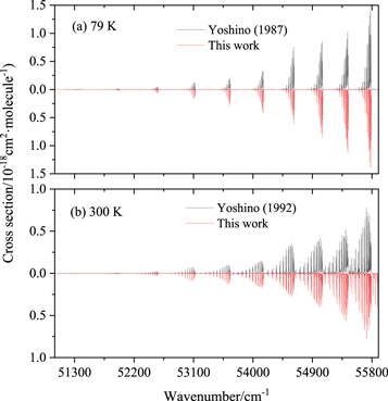
Figure 8. Simulated absorption spectra for the Schumann–Runge bands of O2 at temperatures of (a) 79 and (b) 300 K, respectively. A comparison to the experimental spectra from Yoshino et al. (1987) and Yoshino et al. (1992) is provided. A Gaussian profile of the half-width at half-maximum (HWHM) of 0.9 cm−1 was used.
Download figure:
Standard image High-resolution image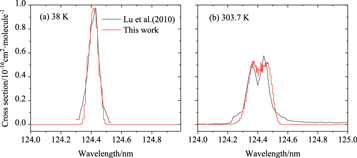
Figure 9. Simulated absorption spectra for the E 
 bands of O2 at temperatures of (a) 38 and (b) 303.7 K, respectively. A comparison to the experimental spectra from Lu et al. (2010) is given. A Gaussian profile of the HWHM of 75 cm−1 was used.
Download figure:
Standard image High-resolution image
Figure 10. Simulated absorption spectra for the E 
 bands of O2 at the temperature of 298 K. A comparison to the experimental spectra from Metzger & Cook (1964) is given. A Gaussian profile of the HWHM of 80 cm−1 was used.
Download figure:
Standard image High-resolution imageTable 2. The Line List for the B 
 Transition
| J' | J'' | Typ | E' | E'' |

|

| State' | υ' | Λ' | Σ' | Ω' | State'' | υ'' | Λ'' | Σ'' | Ω'' |
|---|---|---|---|---|---|---|---|---|---|---|---|---|---|---|---|---|
| 1 | 0 | R | 56,739.2163 | 2.8749 | 56,736.3414 | 6.11E+03 | 2 | 16 | 0 | −1 | −1 | 1 | 0 | 0 | 0 | 0 |
| 1 | 0 | R | 56,341.3890 | 2.8749 | 56,338.5141 | 5.6758E+03 | 2 | 14 | 0 | −1 | −1 | 1 | 0 | 0 | 0 | 0 |
| 103 | 104 | P | 57,396.9447 | 40,714.1649 | 16,682.7798 | 2.9022E+02 | 2 | 0 | 0 | −1 | −1 | 1 | 27 | 0 | 1 | 1 |
| 103 | 104 | P | 57,396.9447 | 41,500.6402 | 15,896.3045 | 3.4896E+01 | 2 | 0 | 0 | −1 | −1 | 1 | 28 | 0 | 1 | 1 |
Notes.
' : upper state.
'' : lower state.
J: total angular momentum.
Typ: transition type.
E: rovibrational energy level.
ν: transition wavenumber.
A: Einstein coefficient.
State: electronic state—2 stands for the B  state and 1 stands for the X
  state.
υ: state vibrational quantum number.
Λ: projection of the electronic angular momentum along the internuclear axis.
Σ: projection of the electronic spin along the internuclear axis.
Ω: projection of the total angular momentum along the internuclear axis, Ω = Λ+Σ.
Only a portion of this table is shown here to demonstrate its form and content. A machine-readable version of the full table is available.
Download table as: DataTypeset image
Table 3. The Line List for the E 
 Transition
| J' | J'' | Typ | E' | E'' |

|

| State' | υ' | Λ' | Σ' | Ω' | State'' | υ'' | Λ'' | Σ'' | Ω'' |
|---|---|---|---|---|---|---|---|---|---|---|---|---|---|---|---|---|
| 1 | 0 | R | 85,660.0515 | 2.8749 | 85,657.1766 | 1.3838E+06 | 2 | 2 | 0 | −1 | −1 | 1 | 0 | 0 | 0 | 0 |
| 1 | 0 | R | 90,138.5898 | 2.8749 | 90,135.7149 | 7.3700E+04 | 2 | 4 | 0 | −1 | −1 | 1 | 0 | 0 | 0 | 0 |
| 103 | 104 | P | 95,504.1824 | 40,714.1649 | 54,790.0175 | 3.7216E+01 | 2 | 0 | 0 | −1 | −1 | 1 | 27 | 0 | 1 | 1 |
| 103 | 104 | P | 95,504.1824 | 41,500.6402 | 54,003.5423 | 8.0825E+01 | 2 | 0 | 0 | −1 | −1 | 1 | 28 | 0 | 1 | 1 |
Only a portion of this table is shown here to demonstrate its form and content. A machine-readable version of the full table is available.
Download table as: DataTypeset image
Figure 11 compares the cross sections for the Schumann–Runge continuum to previous experimental ones from Metzger & Cook (1964), Hudson et al. (1966), Ogawa & Ogawa (1975), Gibson et al. (1983), Yoshino et al. (2005), and Lu et al. (2010). The differences between these experiments are within 10%. Our calculational results agree well with the recent measurements by Lu et al. (2010).

Figure 11. Comparison of the absorption spectrum for the Schumann–Runge continuum to the experimental ones from Metzger & Cook (1964), Hudson et al. (1966), Ogawa & Ogawa (1975), Gibson et al. (1983), Yoshino et al. (2005), and Lu et al. (2010).
Download figure:
Standard image High-resolution imageA comparison of temperature-dependent cross sections for four electronic transitions as a function of photon wavelength at T = 0, 500, 3000, and 10,000 K is shown in Figure 12. For the cross sections at T = 0 and T = 500 K, there is no significant difference, but obvious alterations are seen above T = 3000 K. At long wavelengths, the tails of the cross sections grow because of the more excited rovibrational states at high temperatures. Moreover, the 1 1Πu ←a 1Δg and 1 1Πu ←b 1Σ+ g transitions become more and more important with the temperature increasing.

Figure 12. Photodissociation cross sections for four electronic transitions of O2 including the B 
 and E
and E 
 discrete progressions at (a) T = 0 K, (b) T = 500 K, (c) T = 3000 K, and (d) T = 10,000 K.
Download figure:
Standard image High-resolution image3.3. Photodissociation Rates
Interstellar, solar, and blackbody radiation fields have widespread applications in astrochemistry. We calculated the photodissociation rates of O2 in these three radiation fields. The photodissociation rates of O2 for each transition in the ISRF were calculated using temperature-dependent cross sections and are presented in Table 4. Our calculated photodissociation rate of O2 at T = 0 K is 7.48 × 10⁻¹⁰ s−1, which is slightly lower than that of 7.7 × 10⁻¹⁰ s−1 provided by Heays et al. (2017). Figure 13 shows the photodissociation rates of O2 in the blackbody radiation fields of 4000, 10,000, and 20,000 K, as well as in the solar radiation field. The total photodissociation rates at 0 K are 7.57 × 10⁻¹¹ s−1, 5.66 × 10⁻¹⁰ s−1, and 6.81 × 10⁻¹⁰ s−1 for the blackbody at 4000, 10,000, and 20,000 K, respectively, versus 7.50 × 10⁻¹¹ s−1, 5.60 × 10⁻¹⁰ s−1, and 7.23 × 10⁻¹⁰ s−1 reported by Heays et al. (2017). For the blackbody at 4000 K, the photodissociation rate of O2 increases by nearly 3 orders of magnitude at temperatures from 0 to 10,000 K. However, the photodissociation rates are flattening for the blackbody at 10,000 and 20,000 K, because the radiation fields produced by high-temperature stars tend to flatten the temperature effects on the rates (Pezzella et al. 2022). Our photodissociation rate of O2 in solar radiation fields is 5.87 × 10⁻¹¹ s−1 at T = 0 K, versus 6.10 × 10⁻¹¹ s−1 reported by Heays et al. (2017).

Figure 13. Temperature-dependent photodissociation rates for O2 in the solar radiation field and blackbody radiation fields of 4000, 10,000, and 20,000 K.
Download figure:
Standard image High-resolution image
Table 4. Photodissociation Rates (s−1) of O2 Obtained from Temperature-dependent Cross Sections under the Standard ISRF (Draine 1978; Heays et al. 2017)
| 0 K | 500 K | 1000 K | 2000 K | 3000 K | 5000 K | 10,000 K | |
|---|---|---|---|---|---|---|---|
| 1 1Πu ←a 1Δg | 0 | 5.26E–21 | 4.48E–16 | 1.20E–13 | 7.20E–13 | 2.57E–12 | 4.27E–12 |
1 1Πu ← b 
| 0 | 4.21E–28 | 6.16E–20 | 1.08E–15 | 3.35E–14 | 5.37E–13 | 3.00E–12 |
B 

| 6.71E–10 | 6.72E–10 | 6.85E–10 | 6.65E–10 | 5.95E–10 | 4.83E–10 | 2.86E–10 |
E 

| 7.71E–11 | 7.56E–11 | 7.73E–11 | 8.11E–11 | 8.01E–11 | 6.88E–11 | 3.82E–11 |
| Total | 7.48E–10 | 7.48E–10 | 7.62E–10 | 7.46E–10 | 6.76E–10 | 5.55E–10 | 3.31E–10 |
Download table as: ASCIITypeset image
4. Conclusion
In this work, we have computed photodissociation cross sections and rates of O2 using high-level ab initio PECs and TDMs, which are obtained using the icMRCI+Q/aug-cc-pwCV5Z-DK level of theory. The PECs of the X  and B
and B  states were optimized by the CHIPR method. Discrete progressions of B
 and E
and E 
 were also considered. State-resolved photodissociation cross sections have been computed for four dipole-allowed transitions from the X
  , a 1Δg, and b
  states to excited electronic states. In addition, temperature-dependent cross sections in LTE have been calculated at temperatures from 0 to 10,000 K, assuming the populations of the initial states satisfy a Boltzmann distribution. The photodissociation rates of O2 dissociated through the interstellar, blackbody, and solar radiation fields have been estimated using the temperature-dependent cross sections. The obtained cross sections and rates may contribute to our understanding of the mechanism of oxygen photodissociation in different astronomical environments.
Our photodissociation cross sections of O2 correspond to the absorption spectra for several dipole-allowed transitions. The cross sections for the excitations to the Rydberg states, the predissociations via nonadiabatic couplings, and the magnetic dipole transitions are not considered here. Further analyses of these processes neglected in this work would improve our understanding of the experimental cross sections below 1150 Å (see Figure 7).
Acknowledgments
This work is sponsored by the National Natural Science Foundation of China (52106098, 51421063), the Natural Science Foundation of Shandong Province (ZR2021QE021), the China Postdoctoral Science Foundation (2021M701977), the Postdoctoral Innovation Project of Shandong Province, the Postdoctoral Applied Research Project of Qingdao City, and the Young Scholars Program of Shandong University. The scientific calculations in this paper have been done on the HPC Cloud Platform of Shandong University.
Appendix
The total photodissociation cross sections of O2 at temperatures from 0 to 10,000 K in intervals of 100 K are given in Table 5. The computed photodissociation cross sections of O2 are also available from the ExoMol website: www.exomol.com.
Table 5. The Total Photodissociation Cross Sections (cm2 molecule−1) of O2
| Wavelength | Temperature | ||||
|---|---|---|---|---|---|
| (Å) | 0 K | 100 K | 200 K | 9900 K | 10,000 K |
| 500 | 1.13E–23 | 3.32E–22 | 2.25E–22 | 4.43E–22 | 4.43E–22 |
| 501 | 5.79E–24 | 1.67E–22 | 1.57E–22 | 4.50E–22 | 4.50E–22 |
| 5834 | 0.00E–00 | 7.83E–183 | 4.21E–108 | 6.57E–21 | 6.76E–21 |
| 5835 | 0.00E–00 | 7.49E–183 | 4.12E–108 | 6.60E–21 | 6.79E–21 |
Only a portion of this table is shown here to demonstrate its form and content. A machine-readable version of the full table is available.
Download table as: DataTypeset image